
Submitted:
23 October 2025
Posted:
24 October 2025
You are already at the latest version
Abstract
This study aims to enhance the prediction of bank financial unsoundness by develop-ing an integrated model that combines multiple discriminant analysis (MDA), logit, and probit approaches for Kazakhstan’s banks. Using data from 12 banks between 2008 and 2012, the models were tested on 2013-2014 data, incorporating financial ra-tios that reflect capital adequacy, asset quality, management, earnings, and liquidity. The MDA, logit, and probit models achieved predictive accuracies of 83.3%, 87.5%, and 83.3%, respectively, with Type I errors at 8.3% and Type II errors between 16.7%-25%. The integrated model improved performance, achieving 87.5% accuracy while reduc-ing Type 1 errors to 0%. Since Type I errors – misclassifying unsound banks as sound – pose greater supervisory risk, minimizing them is crucial. The results confirm the su-periority of the logit model and demonstrate that integrating models enhances robust-ness and predictive reliability. The proposed integrated model can serve as a practical tool for supervisory and regulatory authorities to detect potential bank failures early and strengthen financial stability.
Keywords:
banks
; distress
; failure
; MDA
; logit
; probit
; integrated prediction model
; Kazakhstan
1. Introduction
The 2008 financial crisis and its consequences have imposed significant costs on the economies of countries worldwide. Early crisis warning systems in the banking sector proved to be ineffective (Kerstein and Kozberg 2013). The recent failures of Silicon Valley Bank, Signature Bank, and Silvergate Bank have highlighted the necessity to improve tools for identifying troubled banks more promptly (Kabir and Winters 2023).
Factors such as low asset quality, high exposure to market risk, and inadequate internal monitoring have contributed to the vulnerability of banks in Kazakhstan during times of crisis. Predicting and monitoring financially unsound banks is crucial to minimizing the costs of bank failures. This necessitates the use of statistical methods to predict bank failures as early and accurately as possible to allow for timely intervention. Previous studies have primarily focused on developed countries, particularly the USA. There is a lack of research on bankruptcy prediction models in developing countries in general, and post-Soviet countries in particular. Additionally, statistical methods such as MDA, logit, and probit models have been successfully employed in prior studies to predict bankruptcy or bank distress (e.g., Meyer and Pifer 1970; Espahbodi 1991; Catanach and Perry 2001; Canbas, Cabuk, and Kilic 2005; Ioannidis, Pasiouras, and Zopounidis 2010; Betz et al. 2014; Mitchell 2015; and Kimmel, Thornton Jr., and Bennett 2016, Othman 2018; Ekinci and Sen 2023). These studies have confirmed that statistical models have high predictive accuracy in detecting and predicting financial unsoundness.
The purpose of the current study is to employ statistical models to predict bank unsoundness for a sample of Kazakhstani banks and to develop an integrated model to improve the predictability of bank financial unsoundness.
This research examines MDA, logit, and probit statistical models and integrates them to enhance the model's predictive power. For this study, a sample of Kazakhstani banks was taken. The structure of the banking sector was determined using a cluster-based methodology described in the article by Salina, Zhang, and Hassan (2020). Six unsound Kazakhstan banks and six matching sound banks were selected as a sample for this study. Sound banks were selected based on their size (total assets), specialization, and branch networks.
The signaling ability of the MDA, logit, and probit models in predicting the financial unsoundness of banks was assessed. These models identified major indicators of unsoundness in capital adequacy, management, earnings, and liquidity. The predictability of bank failure using these models was enhanced through the calibration of cutoff points by percentile and the combination of all three models into one integrated prediction model. All constructed models exhibited high predictive accuracy. The integrated model minimized Type I errors and demonstrated superior results.
Researchers consider terms such as “unsound,” “problem,” “distressed,” and “failed” as steps leading to bankruptcy. Bankruptcy is the worst-case scenario for an organization, and therefore, the majority of research studies examine this case. “Insolvency,” “failure,” and “default” are other terms with distinct definitions. Altman (1993) posits that all these terms can be combined under the concept of “distress” and share certain common features and signs of potential distress that appear long before bankruptcy. This study aims to develop a model for forecasting financial unsoundness as an earlier step towards distress, reflecting vulnerable and unsafe conditions in Kazakhstan’s banking sector.
The initial studies on analytical coefficients for predicting potential difficulties in the financial performance of companies were conducted in the United States in the early 1930s (Horrigan, 1968). Beaver (1966) and Altman (1968) were pioneers in employing financial ratios and advanced statistical techniques to predict bank bankruptcy or failure. Since then, this approach has gained considerable popularity.
The further development of statistical models for predicting the future status of banks occurred in the 1990s. These models focus on the use of early warning systems. The impetus for studying such models was the wave of bank defaults in the United States in the early 1990s. As a result, statistical models are now used by two regulatory bodies: the Federal Reserve and the Federal Deposit Insurance Corporation (FDIC). These models are known as SEER (System for Estimating Examination Ratings) and SCOR (Statistical CAMELS Off-site Rating).
Bankruptcy forecasting models can be classified into statistical models, artificially intelligent (AI) models, and other models (Aziz and Dar, 2004; Du Jardin, 2009; Citterio, 2024). In their reviews, Aziz and Dar (2004), Du Jardin (2009), and Citterio (2024) provide a critical analysis of the most frequently used bankruptcy forecasting models and compare them in terms of their predictive powers. They concluded that these models are not significantly different from each other in terms of their effect, and that historically, researchers primarily employed statistical models. Aziz and Dar (2004) noted that more than 30% of bankruptcy prediction studies use the MDA model, while another 21% apply the logit model. Together, these models constitute 77% of the statistical models group. Likewise, Bellovary et al. (2007) demonstrated that discriminant analysis, logit analysis, and probit analysis collectively accounted for 61% of their sample, which consisted of bankruptcy studies. Logit and probit analysis belong to the same family of binary choice statistical models, but the probit model is less commonly used. The major difference between these two models lies in their function distributions: it is logistic in the case of the logit model and normal in the case of the probit model. The logit model is more attractive because it is similar to the cumulative normal function but uses simpler calculations.
Recently, academics have been motivated to develop technology-oriented models, such as Artificially Intelligent models, which can be considered a sophisticated automated outgrowth of the statistical approach. Over time, the proportion of studies utilizing statistical methods has decreased due to the emergence of numerous new methods. However, statistical models continue to play a crucial role in predicting bank failures and exhibit a high level of predictive accuracy. Despite this, Aziz and Dar (2004) noted that the superiority of AI models becomes questionable when considering the predictive powers of individual models. In this context, MDA and logit models consistently provide superior predictive accuracies and report low average Type I and Type II error rates.
Khermkhan et al. (2015) compared the forecasting efficiency of the three most popular statistical models. They found that the logit and probit models are flexible and easy to understand and explain. MDA is also an appropriate tool but requires more complex techniques to identify several multivariate groups. Indeed, these classical bankruptcy prediction models have given rise to an extensive body of literature. The MDA, logit, and probit models formed the basis for the vast majority of studies on bank bankruptcy prediction, designing prediction rules and assessing the determinants of financial failure.
Finally, Kimmel (2016) concluded that researchers use statistical methods such as MDA, logit, and probit because they are proven and widely accepted, while newer, more complex models are still under development, with no clear consensus on which version or implementation is superior. Shi, Y., & Li, X. (2019) also identified that the one of the two most frequently used and studied models in bankruptcy prediction area is Logistic Regression. However, most prior studies have been conducted in developed countries, resulting in a lack of evidence about the effectiveness of these models in predicting bank financial unsoundness in developing countries. Therefore, the current study examines the ability of three statistical models to predict bank financial unsoundness in Kazakhstan.
To achieve the purpose of this research, gain insights into the current debate, and identify prominent trends in literature, we have compiled key papers published between 1970 and 2023.
As can be seen from Table 1, these studies cover a publication period from 1970 to 2023. Starting from the 1970s, statistical models like multiple discriminant analysis (MDA), logit analysis, and probit analysis emerged as pioneering techniques for predicting financial distress and were subsequently widely employed in developing bankruptcy prediction models. Generally, statistical methods have been extensively utilized in the literature because of their high interpretability and relatively low computational complexity. Despite dedicated efforts over more than five decades, academics still tend to disagree on which particular models are more reliable, useful, and have higher prediction accuracy for predicting bank unsoundness.
Most of the studies are conducted in developed countries, particularly the USA: Meyer and Pifer (1970), Sinkey (1975), Martin (1977), Bovenzi (1983), West (1985), Espahbodi (1991), Thomson (1991), Bell (1997), Estrella, Park, and Peristiani (2000), Catanach and Perry (2001), Mitchell (2015), Affes and Hentati-Caffel (2016), and Kimmel, Thornton Jr., and Bennett (2016). There are also studies in Europe, such as those by Betz et al. (2014), Filippopoulou, Galariotis, and Spyrou (2020), and Boos et al. (2023). However, there are far fewer studies on developing countries. Examples include Rahman et al. (2004), Canbas, Cabuk, and Kilic (2005), Ioannidis, Pasiouras, and Zopounidis (2010), and Othman (2018). Additionally, Kuznetsov (2003) and Barajas, Krakovich, and López-Iturriaga (2023) used the logit model to predict the default of Russian banks, representing a case of a transition country.
Observed studies utilized either a single prediction model (45%) or two or more models (55%). They employed statistical models such as the MDA model (35%), the logit model (80%), the probit model (20%), and proposed integrated models (20%) to improve the classification accuracy of individual prediction models.
A study by Ioannidis, Pasiouras, and Zopounidis (2010) investigated a sample from several countries and used six quantitative techniques to classify banks into three groups: very strong and strong banks; adequate banks; and banks with weaknesses or serious problems. They compared models developed with only financial variables to models that incorporated regulatory, institutional, and macroeconomic variables. Models using only financial variables exhibited weak prediction accuracy, while the inclusion of country-level variables substantially improved accuracy. The highest accuracy was achieved by models using multi-criteria decision aid and artificial neural networks. Additionally, they developed stacked models that combine the predictions of individual models at a higher level. Although the stacked models outperformed the corresponding individual models.
While Ioannidis, Pasiouras, and Zopounidis (2010) developed a stacked model at a cross-country level, studies by Canbas, Cabuk, and Kilic (2005) and Othman (2018) proposed integrated models using samples from Turkish and Malaysian banks, respectively. Canbas, Cabuk, and Kilic (2005) employed four well-known statistical techniques. Principal component analysis was used to explore the basic financial characteristics of the banks. Based on these characteristics, discriminant, logit, and probit models were developed. The Integrated Early Warning System (IEWS) was effectively employed in bank supervision and could help to avoid bank restructuring costs.
Bagheri et al. (2023) concluded that combining the results of multiple predictive models improves value-at-risk estimation. Citterio (2024), in his review, concluded that ensemble methods, which construct a set of learners and integrate their outputs, achieve reduced variance, improved accuracy, and enhanced model stability, surpassing the performance of individual classifiers. Additionally, current research aims to develop an integrated model, following the approaches of Canbas, Cabuk, and Kilic (2005), Ioannidis, Pasiouras, and Zopounidis (2010), Mitchell (2015), and Othman (2018), to improve the predictability of bank financial unsoundness.
2. Results
2.1. Results: MDA Model
2.1.1. Analysis of the Independent Variables
The purpose of variables analysis is to identify the variables that can efficiently distinguish sound banks from unsound banks. Mean values, standard deviations, Wilk’s Lambda, T, F, and Mann-Whitney U-test results for the fifteen variables are calculated and presented in Table 2.
The Wilk’s lambda is used in discriminant analysis and involves the stepwise inclusion of predictors in the regression equation. It uses the criteria for inclusion of a predictor in the regression equation and the criteria to exclude a predictor from the regression equation.
A two-sample F-test for variances is used to check if the variances of two groups are the same or different, where the null hypothesis H0 is σ1=σ2. Based on the F-test result, an appropriate T-test is then chosen to compare the means. If the p-value from the F-test is smaller than 0.05, H0 is rejected, and the T-test assuming unequal variances is used. If the p-value from the F-test is higher than 0.05, H0 cannot be rejected, and the T-test assuming equal variances is used.
The Mann-Whitney U-test is a non-parametric test used to determine whether two population means are equal. Unlike the t-test and the F-test, it does not require a specific distribution of the dependent variable and is robust against outliers and heavy-tailed distributions.
As seen from Table 5.3, according to the F-tests, seven variables (R1, R2, R3, R5, R12, R13, and R15) were defined as indicators that do not have discriminating power for sound and unsound banks. The T-test selected four insignificant variables: R5, R9, R11, and R15. The Mann-Whitney U-test recognized six variables as significant, with nine variables (R1, R2, R3, R4, R5, R7, R10, R11, and R15) defined as insignificant. Thus, the current research follows the results of the F-test, T-test, and Mann-Whitney U-test given in Table 5.3. The results are ambiguous, which is why all 15 variables were taken into account for the construction of the MDA, logit, and probit models to allow the statistical methods to choose the required variables.
2.1.2. Determination of Discriminant Function Coefficients
Next, discriminant function coefficients are calculated and analyzed. The values of this function should discriminate between the two groups as clearly as possible. A measure of the success of this discrimination is the correlation coefficient between the calculated values of the discriminant function and the group membership indicator. Table 3 shows the canonical correlation coefficient for this study.
In the Function column of Table 3 the value “1” indicates that one discriminant function was obtained in the course of the discriminant analysis. If the dependent variable had not two but three levels, two discriminant functions would be composed.
The high Eigenvalue (0.958) indicates that the obtained model has a high potential for discrimination. Additionally, the high index of canonical correlation (0.700) suggests a close relationship with the variables that define this index.
Table 4 of the Wilks' Lambda lists the indicators that determine the significance of the model obtained because of discriminant analysis.
Wilks’ Lambda is a standard statistic used to denote the statistical significance of discriminating power in the current model. Its value varies from 1.0 (no discrimination) to 0.0 (complete discrimination). Wilks’ Lambda at 0.511 indicates a sufficient level of discrimination
The higher the value of Chi-square, the stronger the discriminant function distinguishes between groups, and the more effectively it fulfills its intended use. The chi-square measure of group overlap indicates that the distributions of the individual vectors of the two groups overlap substantially. Given the high degree of group overlap, the classification results are "better" than might be expected. In this case, the chi-square value is 37.976. Its consistency is demonstrated by statistical significance (Sig.), which in this case is 0.000, and noticeably lower than 0.05.
Table 5 of Standardized Canonical Discriminant Function Coefficients and Table 6 of Structure Matrix allow for the assessment of the correlation of individual independent variables used in the discriminant function with the standardized coefficients. Table 5 summarizes the standardized coefficients, and Table 8 summarizes the correlation coefficients.
Using the standardized coefficients, the relative contribution of each independent variable in the discrimination of the two study groups can be directly compared.
For example, R13 has a stronger effect on the probability of financial unsoundness than R6.

Table 6.
Structure Matrix
| Function | |
| R13 | 0.647 |
| R12a | 0.571 |
| R6a | -0.380 |
| R4a | 0.335 |
| R14 | -0.297 |
| R10a | -0.282 |
| R7a | -0.280 |
| R3a | 0.255 |
| R8 | 0.252 |
| R1a | 0.226 |
| R2a | 0.214 |
| R11a | -0.136 |
| R15a | 0.054 |
| R5a | -0.050 |
| R9a | -0.042 |
- Pooled within-groups correlations between discriminating variables and standardized canonical discriminant functions
- Variables ordered by absolute size of correlation within function.
- a. This variable is not used in the analysis.
Further, the discriminant function coefficients are calculated, and the discriminant equation is derived based on them. These coefficients are included in Table 7.
As a result, given the constant, the discriminant function equation has the following form:
Z=-1.925 + 37.865×R8 + 36.726×R13 - 1.686×R14
Now, based on this equation, the probability that a bank will lose its financial soundness can be calculated.
Table 10 of the Functions at Group Centroids lists the mean values of the discriminant function for each of the analysed groups of the dependent variable.
Table 8.
Functions at Group Centroids
| Status | Function |
| Sound | 0.963 |
| Unsound | -0.963 |
Unstandardized canonical discriminant functions evaluated at group means
Figure 3 shows the point of discrimination between the two groups of financially sound and unsound banks.
Figure 1.
Plot of Bank Centroids with Financially Sound and Unsound Banks
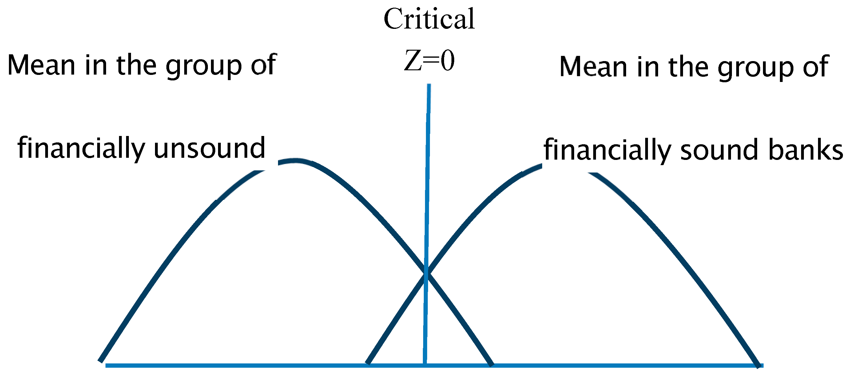
The point for discrimination in the estimated model is 0: if Z is higher than 0, the bank is financially sound; if it is lower, the bank is financially unsound.
2.1.3. Quality Assessment of the Model
The quality of the obtained MDA model was estimated by using an out-sample test with 2013 and 2014 data.
Appendix C shows the assessment of the quality of the model for predicting the financial unsoundness of banks using the constructed MDA model during the out-sample period. Appendix C lists the assigned status Z values calculated by the formula and the predicted status of banks in 2013 and 2014.
As can be seen from Appendix C, the MDA model has predicted the status of financially sound banks for one observation previously defined as financially unsound, such as Kazkommerts bank in 2014. Additionally, it predicted the status of financially unsound banks for three financially sound observations: Halyk Bank of Kazakhstan, SB Sberbank, and Bank Centercredit in 2013.
The classification results are summarized in Table 9 of Classification Results, where the last two rows provide information on the accuracy of predictions.
Based on Table 9 the classification of MDA model errors has been compiled and is presented in Table 10.
Table 10.
Classification of MDA Model Errors 2013 - 2014
| Type of Error |
Number correct |
% correct |
% error |
Total observations |
| Type I | 11 | 91.7 | 8.3 | 12 |
| Type II | 9 | 75.0 | 25.0 | 12 |
| Total | 20 | 83.3 | 16.7 | 24 |
83.3% of original grouped cases correctly classified.
The results of the Multiple Discriminant Analysis in Table 10 show that Type I errors in the out-sample period were 8.3% and Type II errors were 25.0%. The overall accuracy of predictions is 83.3%. The results of the assessment of classification correctness range from 50% to 100%, so the result of 83.3% can be considered more than satisfactory.
2.2. Results: Logit Model
The logistic regression or logit model is a statistical model that can be used to predict the probability of an event by fitting the data to a logistic curve. Using the binary logistic regression the dependence of dichotomous variables on the independent variables that have any kind of scale can be elucidated.
In the case of dichotomous variables, the question is whether a certain event can occur or not. Binary logistic regression, in such a case, calculates the probability of an event occurring based on the values of the independent variables.
The main advantage of using the logit model is that there are no problems with the interpretation of the resulting indicator (p), which can have values ranging from 0 to 1 and determines the nominal value of the probability of a bank's failure.
In discriminant models, the probability of bankruptcy is not determined by a nominal value. Additionally, in discriminant models, there commonly exist so-called “zones of uncertainty,” from which it is impossible to draw an unequivocal conclusion about the probability of bankruptcy based on the calculated indicator.
In the logit models such zones do not exist because, if the assessed probability (p) is greater than 0.5, it is predicted that the event will occur and, if it is less than or equal to 0.5, it is predicted that the event will not occur.
The variables used for building the logit model are the same as those used in the discriminant analysis.
2.2.1. Determination of Logit Model Coefficients
The methods used are Inclusion: Likelihood Ratios (LR) and Exclusion: Likelihood Ratios, which are stepwise. The joint criteria for the coefficients of the model are summarized in Table 13 of the Omnibus Tests of Model Coefficients.
The methods used are the Inclusion: Likelihood Ratios (LR) and the Exclusion: Likelihood Ratios and are stepwise. The joint criteria for the coefficients of the model are summarised in Table 11 of the Omnibus Tests of Model Coefficients.
Chi-Square, step, block, or models are the criteria for the statistical significance of the effects on the dependent variable of all predictors in a specified model, block, or step. In step 1, all three criteria of Chi-square are equal for models and steps because, at step 1, they are identical for block and model as the model contains only one block. Large values of the Chi-square criterion indicate that all included variables have a significant effect on the dependent variable.
The parameters to assess the likelihood of the model accuracy are summarised in Table 12.
The value of the -2 Log Likelihood describes the model and shows how well it matches the original data. Cox and Snell's R square and Nagelkerke R square are approximations of the R value, indicating the proportion of the impact of all predictors of the model on the variance of the dependent variable.
In this study, Nagelkerke R square is 0.723, meaning that the behaviour of the dependent variable is explained at a level of 72.3% by the predictors included in the model.
Table 13 shows the effects of the inclusion of variables in the equation at each step of its compilation. The line Constant for each step corresponds to the constant a of the regression equation.
Table 13.
Omnibus Tests of Model Coefficients
| B | S.E. | Wald | df | Sig. | Exp(B) | ||
| Step | R5 | -0.516 | 0.296 | 3.033 | 1 | 0.082 | 0.597 |
| 1 | R8 | -245.762 | 101.767 | 5.832 | 1 | 0.016 | 0.000 |
| R13 | -119.94 | 41.915 | 8.188 | 1 | 0.004 | 0.000 | |
| R14 | 3.804 | 1.366 | 7.758 | 1 | 0.005 | 44.898 | |
| Constant | 9.794 | 3.476 | 7.938 | 1 | 0.005 | 17931.929 |
a. Variable(s) entered on step 1: R5, R8, R13, R14
Wald chi-square tests the null hypothesis that the B coefficient or constant equals 0. If the p-value from the column Sig. is less than 0.05, the hypothesis is rejected, and the B coefficient or constant is not 0. Exp(B) is an odds ratio and is the exponentiation of the B coefficient. P values for all ratios and the constant are less than 0.05. Based on the Wald chi-square test and its p-value (Sig.), all coefficients of the logit model are statistically significant. Thus, equation Z will be:
Zlfs = -0.516×R5-245.762×R8-119.94×R13+3.804×R14+9.794
2.2.2. Assessment of Logit Model Quality
An out-sample test with 2013 and 2014 data was applied to assess the quality of the constructed logit model. The calculated probability values and the prediction of distribution into groups are listed in Appendix D.
As can be seen from Appendix D, the logit model has predicted the status of financially sound banks for one case previously defined as financially unsound, such as TemirBank in 2014. It also predicted the status of financially unsound banks for two financially sound observations: Halyk Bank of Kazakhstan and Bank Centercredit in 2013.
The comparison of predicted values for the dependent variable based on the logit model and the assigned status is shown in Classification Table 14.
As the data in the last column of the Table 15 show, the results of prediction proved to be correct for 87.5% of objects. It is more convenient to interpret the results in the form of the following indicators in Table 15.
Table 15 shows that Type I errors are 8.3% and Type II errors are 16.7%. A total of 87.5% of cases are classified correctly. The predictive ability of the model is high.
This section may be divided by subheadings. It should provide a concise and precise description of the experimental results, their interpretation, as well as the experimental conclusions that can be drawn.
2.3. Results: Probit Model
In probit analysis, the probability of banks falling into one of two groups is presented as a function of the normal distribution:
2.3.1. Determination of Probit Model Coefficients
The statistics provided in Table 16 generated in Eviews will help to assess the quality of the model; coefficients for the calculation of Zpa are also provided there.
Table 16 includes the statistics, which can be used to assess the significance of the probit model. All coefficients of the probit model are statistically significant, as seen from the z-statistics.
Zpa = 3.247906 -75.34322 x R8 - 65.96576 × R13 + 2.474162 × R14
When determining the predicted status, the probit model calculates the probability for each object and, based on this probability, assigns one of the two values of the dichotomous variable to a bank. If the probability is less than 0.5, the bank is assessed as financially sound (the value of the variable "status" is set to 0); otherwise, the bank is considered financially unsound (the value of the variable "status" is set to 1).
2.3.2. Assessment of Probit Model Quality
The values of Zpa, the probability, and the status of banks calculated for the out-sample period 2013-2014 based on the constructed probit model are listed in Appendix E.
As seen from Appendix E, the probit model has predicted the status of financially sound banks for one case previously defined as financially unsound, such as Kazkommerts bank in 2014. It also predicted the status of financially unsound banks for three financially sound observations: Halyk Bank of Kazakhstan, SB Sberbank, and Bank Centercredit in 2013.
The quality of the assessed probit model and the correctness of classification for 2013–2014 are summarized. Based on the predicted status and the percentage of correct observations, the classification of errors in the out-sample period is compiled in Table 17.
Thus, the probit model has 8.3% of Type I errors and 25.0% of Type II errors in the 2013–2014 period. A total of 83.3% of the observations are classified correctly. This indicates a high predictive ability of the probit model during the out-sample period.
In summary, both the MDA and probit models exhibited high predictive accuracy of 83.3% during the out-of-sample period. The logit model outperformed the others, achieving a predictive accuracy of 87.5%. Furthermore, Khashei, Etemadi, and Bakhtiarvand (2024) demonstrated that the newly developed discrete direction-based logistic regression, a widely used statistical classifier for bankruptcy forecasting, provides an efficient and robust approach for achieving superior predictive performance.
The high predictive accuracy of these models is satisfactory. Nevertheless, the cut-off points were adjusted to improve the models’ performance, and the results of the three models were combined and reported in Table 18.
The new cut-off points improved the quality of all models. The predictive ability of the MDA model increased from 83.3% to 87.5%, Type II errors decreased from 25.0% to 16.7%, and Type I errors remained unchanged. The predictive accuracy of the logit model improved from 87.5% to 91.67%, with Type II errors remaining at 16.7% and Type I errors decreasing from 8.3% to 0%. Most significantly, the predictive ability of the probit model improved from 83.3% to 95.83%, with Type II errors decreasing from 25.0% to 0% and Type I errors remaining at 8.3%.
2.4. Results: Integrated Prediction Model of Bank Unsoundness
Research devoted to enhancing the prediction models has increased, and some studies integrating and comparing two or more models have appeared. Lee (1990) was one of the first researchers who integrated two models in decision support systems and noted that integration can synergistically benefit both. He affirmed that integration implies the unification of problem specifications and solution procedures, which encompass both integrating methodologies. Jo and Han (1996) suggested the use of an integrated model that used a combination of discriminant analysis, neural networks, and a case-based forecasting system. They used bankruptcy prediction to validate the effectiveness of the integrated model, and the prediction ability of the integrated model was superior to the three independent prediction techniques. They concluded that prediction error was reduced when the prediction results of various methods were combined.
Also, Lam and Moy in 2002 presented a method which combines several discriminant methods to predict the classification of new observations. They drew conclusions that as, no single-discriminant method outperforms other discriminant methods under all circumstances, decision-makers may solve a classification problem using several discriminant methods and examine their performance for classification purposes in the training sample.
The current study tries to improve the predictability of the three empirical models (MDA, logit, and probit) obtained above. They can be systematically combined to construct an integrated prediction model of bank financial unsoundness as a reliable decision tool in bank supervision and examination. This model could help increase the probability of correct forecasting.
Figure 2 shows the structure of the integrated prediction model of bank financial unsoundness and its data flow. Basically, the predicted values from the three models are employed as the input variable of the integrated model. The processes of the integrated model are presented in the view of the data flow. The model consists of four types of data: (i) four variables, (ii) computed coefficients of MDA, logit, and probit models, (iii) predicted values of the discriminant score by the MDA model and probabilities by the logit and probit models, and (iv) prediction output (sound/unsound bank).
When assessing a new bank according to the integrated model, all the system data will remain unchanged, except for the four financial ratios of the analyzed bank. These ratios are the basis for the MDA, logit, and probit models. Hence, the input to the system consists of four ratios, which are used in calculating the discriminant score and the logit and probit probabilities of bank unsoundness. The system provides early warning signals for each of the discriminant, logit, and probit models. These three empirical models together increase prediction accuracy regarding the future problems of the bank. The integrated model assigns an unsound status to a bank if even one of the three models predicts the bank as unsound.
For example, the estimated discriminant score for Kazkommerts bank on 1st January 2014 is 0.096, which is lower than the cut-off score. The estimated logit and probit unsoundness probabilities for this bank are 69.0% and 44.3%, respectively. According to the MDA and probit models, this bank is sound; according to the logit model, it is unsound. Thus, the logit model gives true information about this bank, which was actually unsound in 2014. The integrated model also assigns the status of unsound to this bank. Therefore, the integrated model provides more cautious and conservative forecasts that should reduce Type I errors. The ability to detect bank unsoundness will reduce the cost of monitoring and provide valuable information to the supervisor to prevent bank failure.
The integrated model determined the predicted statuses for each case from 1st January 2013 to 1st January 2014, as presented in Appendix F.
As can be seen from Appendix F, the integrated model has predicted the status of financially unsound for three financially sound observations: Halyk Bank of Kazakhstan, SB Sberbank, and Bank Centercredit in 2013.
The classification results of the integrated model on out-sample data for predictive accuracy, Type I errors, and Type II errors are shown in Table 19.
Table 19 shows that the predictive accuracy of the integrated model in the out-sample period is high. Type I errors are absent, and Type II errors are 25.0%. A total of 87.5% of cases are classified correctly. The integrated model did not outperform the MDA model in overall predictive accuracy. However, it reduced the rate of Type I errors compared to the MDA, logit, and probit models. As is known, Type I errors are more costly than Type II errors.
3. Discussion
We illustrate the usefulness of the integrated model to predict bank unsoundness by comparing its predictive accuracy. The comparative analysis starts by examining the accuracy of the models in predicting bank unsoundness that occurred during the sample period. This study focused on three statistical models in an attempt to evaluate their effectiveness with respect to each other, in addition to an integrated model based on all three. Four criteria will be used to assess the performance of these models, namely:
- percentage of Type I errors;
- percentage of Type II errors; and
- predictive ability of the model.
This section analyzes the predictive ability of the three empirical models and the integrated model. Prior studies conclude that integrated models produce higher prediction accuracy than individual models (Jo and Han, 1996). Results from this study are in line with these findings (Table 20).
All employed models demonstrated high overall predictive accuracy in 2013–2014. The MDA and probit models had an accuracy of 83.3%, while the logit and integrated models achieved 87.5%. The integrated model showed the lowest rate of Type I errors at 0.0%. The logit model had the lowest rate of Type II errors at 16.7%. The MDA, probit, and logit models' Type I errors were 8.3%, and the Type II errors were 25.0% for the MDA and probit models, and 16.7% for the logit model. The integrated model had the expected lowest rate of Type I errors at 0.0% and Type II errors at 25.0%. All models were effective in predicting the unsoundness status of banks, but the integrated model slightly outperformed the MDA, logit, and probit models in reducing Type I errors.
The loss from Type I errors is significantly larger than that of Type II errors because a Type I error occurs when a bank predicted to be financially sound defaults, while a Type II error implies that a bank predicted to be financially unsound survives. Sahajwala and Van den Berg (2000) confirm that Type I error is potentially more serious than Type II error because a weak bank that may escape supervision entails a higher risk. Supervisory authorities aim at minimizing the Type I error rate and calibrating models to carry a low Type I error. Therefore, the integrated model demonstrated superior results, reducing Type I errors to 0.0%.
Jo and Han (1996), Lam and Moy (2002), Canbas, Cabuk, and Kilic (2005), and Othman (2013) affirmed that combining several models provides superior information about future prospects. The results of this study show that an integrated model decreases Type I error.
Indeed, two approaches—discriminant analysis and choice models—are often compared in terms of predictive power in prior studies. Lennox (1999) and Lin (2009) noted the superiority of the logit model, while Altman et al. (1994) and Jagtiani (2003) did not find a significant difference in the predictive power of the two approaches. The results of the current study are consistent with both findings because the predicted values of these models are very close, but the predictive power of the logit model is slightly higher.
This study concludes that an integrated model can serve as an effective and cost-efficient supervisory tool, capable of identifying unsound banks over extended periods without the need for modification. This implies that the signal indicators employed by such models must remain stable over time. Furthermore, the study finds that all the examined models efficiently detect signs of bank unsoundness within a five-year horizon and can therefore be considered reliable predictive techniques. Although Bro de Comères (2025) argues that a period of four quarters preceding actual distress events is sufficiently long to enable policymakers to take preventive action once a distress signal has been issued, while at the same time limiting the likelihood of reverse causality bias.
The power of these empirical models lies in the indicators used by them. Focusing on the ability of financial ratios to highlight banks vulnerable to financial distress, the four variables reflecting capital adequacy, management, operating efficiency, and liquidity were chosen. In the models using the MDA, logit, and probit analysis, the significant coefficients calculated were the R13 interest rate spread and the R14 working capital to total assets ratio. The MDA and logit analysis consider one more ratio, R8 salary to assets. Additionally, the logit model considers the R5 debt to equity ratio.
The R13 interest rate spread is calculated as the difference between the average interest rate paid to depositors and the average interest rate earned from borrowers. This indicator reveals bank operating efficiency and allows a superior understanding of the sources of bank profitability, and hence the degree of vulnerability of its profitable sources. A negative or very low value indicates an ineffective interest rate policy or a loss, but a high value could also be a negative sign because high rates are often earned on assets that are excessively risky.
The R14 net working capital to total assets ratio is used to measure liquidity. It is an indicator from the modified Altman four-factor model for non-manufacturing companies. It is calculated as the ratio of net working capital to total assets. Working capital is the difference between current assets and current liabilities. Altman (1968) considered this indicator as the most valuable of the three liquidity ratios.
Rahman et al. (2004) proved that capital adequacy, loan management, and operating efficiency are three common performance dimensions able to identify problem banks. This result comes as no surprise, as banks with a high R5 debt to equity ratio are more fragile during crises. Estrella, Park, and Peristiani (2000) suggest using simple coefficients such as leverage to predict bank failure, as it is a very informative indicator. Also, sometimes less frequently mentioned indicators have a higher ability to discriminate depending on the particular situation and may change over time (Ohlson, 1980). In this case, they include the R8 salary to assets ratio.
These four early indicators could provide supervisory bodies with a head start in identifying the root causes of changes in a bank’s financial soundness and could potentially enhance the effectiveness of off-site monitoring. Understanding the root causes of a bank’s unsoundness is likely to improve the overall effectiveness of bank monitoring and supervision.
4. Materials and Methods
This study utilizes statistical models to predict bank financial unsoundness, specifically using MDA, logit, and probit analyses. It employs a set of indicators selected and analyzed in Salina, A.P., Zhang, X., and Hassan, O.A.G. (2020). It seeks to answer the following research question:
Can the predictability of bank financial unsoundness be improved by using statistical models such as MDA, Logit and Probit?
To achieve this goal, the predictability of these models is investigated, and then an integrated model using MDA, logit, and probit analyses is developed. The logic behind this approach is that the integration of several simple models into a more complex one is easier than building a single complex model (Ferreira and Figueiredo, 2012).
Figure 1.
Process and Design of Integrated Prediction Model of Bank Unsoundness
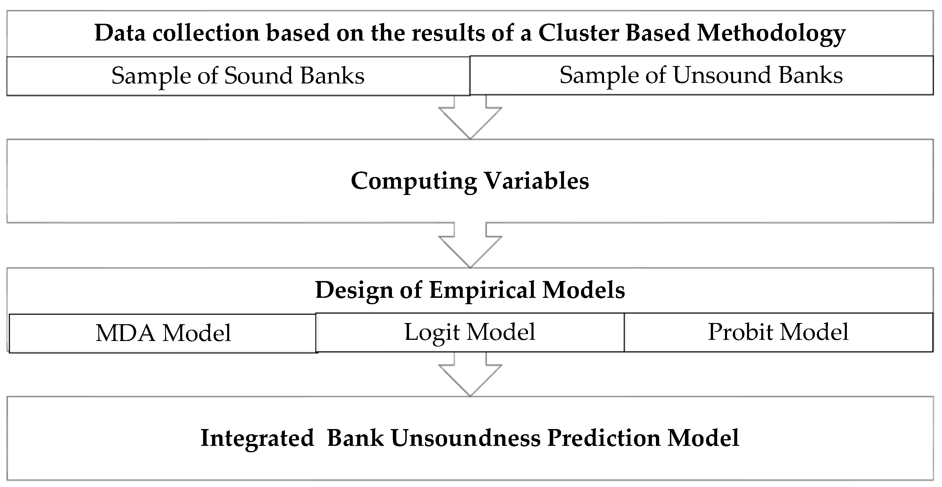
The process starts with data collection. Our sample consists of 12 banks: six unsound and six sound banks. The status of unsound banks was assigned by cluster analysis on January 1, 2014, as described in Salina, Zhang, and Hassan (2020). The six sound banks were matched from a group of financially sound banks based on asset size, specialization, and branch network. The entire sample comprises 12 banks, representing 81.3% of the total assets in the banking sector (Table 2).
Table 2.
Selected Sample of Banks and Asset Share, 1st January, 2014
| Unsound Bank | Share in Assets of Banking Sector, % | Ranking | Sound Bank | Share in Assets of Banking Sector, % |
| Kazkommertsbank | 16.2 | 1 | Halyk Bank of Kazakhstan | 15.8 |
| BTA Bank | 9.8 | 2 | Bank Centercredit | 6.9 |
| ATF Bank | 5.8 | 3 | SB Sberbank | 6.7 |
| Alliance Bank | 3.6 | 4 | Tsesnabank | 6.0 |
| Temirbank | 2.0 | 5 | Kaspi Bank | 5.5 |
| Total | 39 | 42.3 | ||
| Total of two groups | 81.3 |
Variables used in this study were carefully chosen and analyzed in the descriptive statistics in Salina, Zhang, and Hassan (2020) (Table 3).
The next step involves selecting indicators based on a review of relevant prior studies. In this study, accounting-based variables were chosen as indicators due to their proven high predictive ability. Citterio (2024) concluded that, although the predictive accuracy of macroeconomic information has been examined in several studies, there is only limited evidence regarding the influence of non-financial performance on a bank’s probability of default.
Following the CAMELS acronym, indicators were selected to reflect the main characteristics of capital adequacy, asset quality, management, earnings, and liquidity (Table 3). These 15 variables are widely used in studies devoted to bank financial soundness, distress, failure, and bankruptcy, and they reflect the nature of the banking sector.
Table 2.
Description of Selected Financial Ratios
| Code | Ratio | Measurement | |
| Capital Adequacy | R1 | Capital adequacy ratio (CAR) | Equity / Total Assets |
| R2 | Regulatory capital to risk-weighted assets | Regulatory Capital / Risk-Weighted Assets | |
| R3 | Regulatory Tier 1 capital to risk-weighted assets | Tier 1 Regulatory Capital / Risk Weighted Assets | |
| R4 | Equity to debt ratio | Book Value Equity / Book Value of Total Liabilities | |
| R5 | Debt to equity ratio (financial leverage) | Total Liabilities / Total Equity | |
| Asset Quality | R6 | Nonperforming loans to total gross loans ratio | Value of NPLs / Total Value of the Loan Portfolio |
| R7 | Nonperforming loans net of provisions to capital ratio | (NPLs - the Value of Specific Loan Provisions) / Total Regulatory Capital | |
| Management | R8 | Salary to assets ratio | Gross Salary Accrued / Total Assets |
| Earnings | R9 | Return on assets (ROA) | Earnings after Tax / Total Assets |
| R10 | Return on equity (ROE) | (Gross Income - Gross Expenses) / Average Value of Capital | |
| R11 | EBIT to total assets ratio | Earnings Before Interest and Tax / Total Assets | |
| R12 | Net interest margin | (Interest Income - Interest Expenses) / Earning Assets | |
| R13 | Interest rate spread | Lending Rate – Deposit Rate | |
| Liquidity | R14 | Working capital to total assets ratio | (Current Assets – Current Liabilities) / Total Assets |
| R15 | Current ratio | Average Current Assets / Average Demand Deposit Liabilities |
As seen from Table 3, these 15 variables are widely used in studies devoted to bank financial soundness, distress, failure, and bankruptcy, reflecting the nature of the banking sector. For instance, Guillen (2025), in assessing the main factors that led to the collapse of Silicon Valley Bank and First Republic, found that capital adequacy, management quality, earning ability, and liquidity position ratio can predict bank failure up to five years before the official bankruptcy. Guillen’s study highlights the importance for policymakers to closely monitor these financial indicators to prevent potential bank runs and financial crises. They are also part of the IMF’s Financial Soundness Indicators (FSI) (R1, R2, R3, R6, R7, R9, R10, and R15) and the prudential norms of Kazakhstan banks (R1, R2, R3, R5, R6, R7, R10, R12, R13, and R15).
This set of 15 selected indicators was used in Salina, Zhang, and Hassan (2020) to identify the structure of the Kazakhstan banking sector by degree of financial soundness. In Salina, Zhang, Tong, and Hassan (2023), indicators R4, R9, R11, and R14 were used to test the ability of Altman’s models to predict bank financial unsoundness. This research employs the set of 15 financial ratios to construct prediction models of bank financial unsoundness using MDA, logit, and probit techniques.
Thus, the MDA, logit, and probit models are employed on a sample of 12 Kazakhstan banks annually from January 1, 2008, to January 1, 2014. Since sound and unsound groups of banks were defined on January 1, 2014, this date serves as the benchmark. This sample was divided into in-sample and out-sample groups. The first group was used for the models’ design, while the second group was used to check the models’ ability to predict financial unsoundness. The in-sample period consists of observations from January 1, 2008, to January 1, 2012, while the out-sample period includes January 1, 2013, and January 1, 2014. A set of fifteen financial ratios used in Salina, Zhang, and Hassan (2020) were computed annually for the period from January 1, 2008, to January 1, 2014 (Appendix A, Appendix B).
MDA analysis, based on certain features (independent variables), assigns the object to one of two (or a few) pre-set groups. This setting of the problem, especially in the case of two predefined groups, closely resembles the problem statement for the logistic regression method. The core of discriminant analysis is the construction of the so-called discriminant function.
where
D = β1Х1 + β2Х2 + ... + BnХn + α,
D – the discriminant value;
X1 and Xn — the values of variables relevant to the cases under consideration;
β1 – βn — the coefficients to be assessed using the discriminant analysis; and
α – the constant.
The purpose is to determine such coefficients that would enable partitioning into groups with maximum accuracy based on the discriminant function values.
The logit model is used to predict the probability of an event by fitting the data to a logistic curve. Using binary logistic regression, the researcher can explore the dependence of dichotomous variables on independent variables that have any scale.
Commonly, a dichotomous variable refers to an event that may or may not occur; binary logistic regression, in such a case, estimates the probability of the event occurrence based on the values of independent variables.
The probability of event occurrence for some cases shall be calculated by the formula.
where
where
z= β1Х1 + β2Х2 + ... + BnХn + α,
X1 and Xn — the values of variables relevant to the cases under consideration
β1 – βn — the factors to evaluate and
α – error term (the probability of Type I error occurs).
The advantage of using logit models is that there are no problems with the interpretation of the resulting indicator (R), which takes on values only in the range from 0 to 1 and determines the nominal value of the probability of entity insolvency. In logit models, such zones are absent because if the estimated probability (R) is more than 0.5, it is predicted that the event will occur, and if it is less than or equal to 0.5, the event will not occur.
For the calculation of factors in the model, methods of Inclusion: Likelihood Ratios (LR) and Exclusion: Likelihood Ratios are used, which are stepwise. Quality assessment of the model is made by calculating multiple indicators. The Log Likelihood value describes the model and shows how well it matches the original data. Cox and Snell's R square and Nagelkerke’s R square are approximations of the R-square values, indicating the share of influence of all predictors of the model on the variance of the dependent variable.
The probit model is a statistical non-linear model used in various areas, providing a method for analyzing the dependence of qualitative variables on a set of factors based on normal distribution. In econometrics, probit models are employed in models of binary or multiple choice between different alternatives to model default rates of companies.
The term "probit" is derived from the English “probability unit” and was introduced by Chester Ittner Bliss [1899—1979]. The probit model allows for the estimation of the probability that the analyzed (dependent) variable takes the value 1 at pre-set values of factors (an estimation of the share of "units" at a given value of factors). In the probit model, the probit function is modelled as a linear combination of factors, including a constant.
In probit analysis, the probability of banks falling into one of the two groups is presented as a function of the normal distribution.
where Zpa equation takes the following form:
where
Zpa = β1Х1 + β2Х2 + ... + BnХn + α,
X1 and Xn — the values of variables relevant to the cases under consideration
β1 – βn — the factors to evaluate and
α – error term.
Logit and probit models are very similar as both are models of binary choice. The difference between the models lies in the distribution of the error term. If the error term has a standard normal distribution, the probit model should be used. If the error term has a logistic distribution, the logit model should be used.
To increase the predictability of MDA, logit, and probit models, an approach by Begley et al. (1996) and Wu et al. (2010) was used. The obtained discriminant score and probabilities from logit and probit analysis were ranked from lowest to highest. It was assumed that the superior cut-off point lies between the 25th and 75th percentiles. The cut-off points were selected as the percentile at which the sum of Type I and Type II classification errors was minimized and the predictive ability was highest.
Finally, as a concluding step, a comparison between the outcomes of all empirical models employed in this study is developed for the MDA, logit, probit, and integrated models. The comparative analysis focused on four features: the percentage of Type I errors, the percentage of Type II errors, the predictive ability of the model, and the prediction accuracy annually. Type I error represents the misclassification of an unsound bank as sound. Conversely, Type II error is a statistical term identified with misclassification by a model when the system wrongly classifies a sound bank as unsound (Sahajwala and Van Den Bergh, 2000).
5. Conclusions
This study analyzed the ability of three statistical models in predicting the financial soundness of banks, namely the MDA, logit, and probit models. In addition, it developed an integrated model based on these three models. Firstly, the explanatory power of the independent variables and the correlation between them were assessed. Next, the MDA, logit, and probit models were constructed and integrated to find the most reliable model by exploring their predictive ability. Finally, a comparative analysis of the predictive ability of the empirical models was carried out.
The empirical results of this study are listed as follows:
1. In the out-sample period, the MDA model predicted the status of financial soundness for one observation previously defined as a financially unsound bank, such as Kazkommerts bank in 2014, and the status of financial unsoundness for three financially sound observations: Halyk Bank of Kazakhstan, SB Sberbank, and Bank Centercredit in 2013.
For the Multiple Discriminant Analysis model, in the out-sample period in 2013–2014, Type I errors in the model were 8.3% and Type II errors were 25.0%. The overall accuracy of predictions is 83.3%.
2. The logit model predicted the status of financial soundness for one case previously defined as a financially unsound bank, such as TemirBank in 2014, and the status of financial unsoundness for two financially sound observations: Halyk Bank of Kazakhstan and Bank Centercredit in 2013.
Type I errors are 8.3% and Type II errors are 16.7% in the out-sample period in 2013–2014. A total of 87.5% of cases are classified correctly. The predictive ability of the model is high.
4. The probit model predicted the status of financial soundness for one case previously defined as a financially unsound bank, such as Kazkommerts bank in 2014, and the status of financial unsoundness for three financially sound observations: Halyk Bank of Kazakhstan, SB Sberbank, and Bank Centercredit in 2013.
The probit model has Type I errors at 8.3% and Type II errors at 25.0%. In general, 83.3% of observations have been classified correctly in 2013–2014.
5. The integrated model predicted all unsound banks correctly, but it assigned the status of financial unsoundness to three financially sound observations: Halyk Bank of Kazakhstan, SB Sberbank, and Bank Centercredit in 2013.
In 2013–2014, the integrated model had no Type I errors and its Type II errors were at 25.0%. A total of 87.5% of cases were classified correctly.
6. All constructed models demonstrated high predictive ability. The logit and integrated models had superior overall predictive ability to forecast bank financial unsoundness compared to the MDA and probit models. The predictive ability of the integrated model was equal to the logit model, but it proved its superiority in reducing Type I errors. This research has confirmed the conclusions of Jo and Han (1996), Canbas, Cabuk, and Kilic (2005), and Othman (2013) that when the prediction results of various methods were combined, the prediction accuracy improved.
Author Contributions
Conceptualization, Aigul Salina; methodology, Aigul Salina; software, Aigul Jondelbayeva; validation, Aigul Salina, Omaima Hassan and Xing Zhang; formal analysis, Aigul Salina; investigation, Aigul Jondelbayeva, resources, Aigul Salina, Omaima Hassan and Xing Zhang; data curation, Aigul Jondelbayeva; writing — original draft preparation, Aigul Salina; writing — review and editing, Aigul Jondelbayeva, Omaima Hassan and Xing Zhang; visualization, Aigul Jondelbayeva; supervision, Omaima Hassan and Xing Zhang; project administration, Aigul Salina and Aigul Jondelbayeva; funding acquisition, not applicable. All authors have read and agreed to the published version of manuscript.
Funding
“This research received no external funding”
Data Availability Statement
All data used in article is secondary. The data presented in this study are publicly available from official open sources, including the website of the National Bank of Kazakhstan (https://www.nationalbank.kz), the Kazakhstan Stock Exchange (KASE) (https://kase.kz), and the official websites of commercial banks operating in Kazakhstan. All data were accessed between January 2014 and December 2017.
Acknowledgments
The authors would like to express their gratitude to the supervisors for their academic guidance and constructive feedback during the research process. No external funding or material support was received for this study. The authors prepared and wrote this manuscript independently.
Conflicts of Interest
“The authors declare no conflicts of interest.”
Abbreviations
The following abbreviations are used in this manuscript:
| MDA | Multiple Discriminant Analysis |
Appendix A
Table A.
Data for MDA, Logit and Probit Analyses (in sample).
| Banks | Year | Status | R1 | R2 | R3 | R4 | R5 | R6 | R7 | R8 | R9 | R10 | R11 | R12 | R13 | R14 | R15 |
| Bank Centercredit | 2008 | 0 | 0,122 | 0.073 | 0.128 | 0.133 | 7.529 | 0.01 | 0.059 | 0.008 | 0.016 | 0.128 | 0.058 | 0.026 | 0.024 | -0.644 | 1.297 |
| Bank RBK | 2008 | 0 | 0.83 | 0.689 | 0.868 | 4.895 | 0.204 | 0 | 0 | 0.044 | 0.013 | 0.015 | 0.007 | 0.088 | 0.088 | 0.566 | 0.957 |
| Halyk Bank of Kazakhstan | 2008 | 0 | 0.112 | 0.07 | 0.12 | 0.123 | 8.151 | 0.019 | 0.117 | 0.01 | 0.021 | 0.187 | 0.057 | 0.031 | 0.028 | -0.127 | 1.192 |
| Kaspi Bank | 2008 | 0 | 0.142 | 0.089 | 0.128 | 0.161 | 6.222 | 0.034 | 0.178 | 0.019 | 0.023 | 0.159 | 0.06 | 0.068 | 0.063 | -0.577 | 1.38 |
| SB Sberbank | 2008 | 0 | 0.636 | 0.496 | 0.482 | 1.5 | 0.667 | 0.039 | 0.036 | 0.021 | 0.021 | 0.034 | 0.046 | 0.046 | 0.038 | 0.451 | 1.736 |
| Tsesnabank | 2008 | 0 | 0.155 | 0.112 | 0.14 | 0.178 | 5.626 | 0.015 | 0.074 | 0.021 | 0.007 | 0.045 | 0.053 | 0.025 | 0.022 | -0.39 | 1.156 |
| Alliance Bank | 2008 | 1 | 0.156 | 0.113 | 0.143 | 0.18 | 5.557 | 0.014 | 0.063 | 0.008 | 0.031 | 0.2 | 0.078 | 0.048 | 0.045 | 0.051 | 3.009 |
| ATF Bank | 2008 | 1 | 0.131 | 0.085 | 0.142 | 0.142 | 7.033 | 0.01 | 0.061 | 0.006 | 0.006 | 0.047 | 0.047 | 0.02 | 0.018 | -0.36 | 1.594 |
| BTA Bank | 2008 | 1 | 0.179 | 0.136 | 0.138 | 0.211 | 4.732 | 0.006 | 0.025 | 0.006 | 0.018 | 0.103 | 0.054 | 0.023 | 0.02 | -0.525 | 1.485 |
| Kazkommertsbank | 2008 | 1 | 0.132 | 0.083 | 0.123 | 0.146 | 6.827 | 0.022 | 0.137 | 0.004 | 0.017 | 0.129 | 0.053 | 0.028 | 0.025 | 0.444 | 1.35 |
| Nurbank | 2008 | 1 | 0.223 | 0.173 | 0.209 | 0.275 | 3.636 | 0.023 | 0.075 | 0 | 0.015 | 0.067 | 0.049 | 0.016 | 0.011 | -0.164 | 1.61 |
| Temirbank | 2008 | 1 | 0.166 | 0.141 | 0.141 | 0.199 | 5.024 | 0.026 | 0.131 | 0.013 | 0.025 | 0.149 | 0.079 | 0.039 | 0.034 | 0.237 | 1.558 |
| Bank Centercredit | 2009 | 0 | 0.154 | 0.103 | 0.186 | 0.171 | 5.863 | 0.024 | 0.108 | 0.01 | 0.006 | 0.066 | 0.091 | 0.026 | 0.025 | -0.651 | 0.295 |
| Bank RBK | 2009 | 0 | 0.903 | 0.744 | 0.911 | 9.354 | 0.107 | 0 | 0 | 0.082 | 0.011 | 0.012 | 0.014 | 0.088 | 0.087 | 0.879 | 6.096 |
| Halyk Bank of Kazakhstan | 2009 | 0 | 0.128 | 0.086 | 0.123 | 0.143 | 7.017 | 0.043 | 0.256 | 0.009 | 0.006 | 0.058 | 0.072 | 0.029 | 0.028 | 0.068 | 1.274 |
| Kaspi Bank | 2009 | 0 | 0.152 | 0.113 | 0.141 | 0.173 | 5.781 | 0.046 | 0.226 | 0.018 | 0.005 | 0.042 | 0.097 | 0.055 | 0.052 | -0.807 | 0.13 |
| SB Sberbank | 2009 | 0 | 0.378 | 0.327 | 0.41 | 0.582 | 1.717 | 0.045 | 0.094 | 0.021 | 0.024 | 0.068 | 0.089 | 0.048 | 0.038 | 0.173 | 1.108 |
| Tsesnabank | 2009 | 0 | 0.139 | 0.1 | 0.129 | 0.157 | 6.387 | 0.041 | 0.194 | 0.023 | -0.043 | -0.378 | 0.042 | 0.024 | 0.022 | -0.58 | 0.393 |
| Alliance Bank | 2009 | 1 | 0.185 | 0.166 | 0.193 | 0.219 | 4.572 | 0.033 | 0.12 | 0.009 | 0.001 | 0.01 | 0.084 | 0.042 | 0.038 | 0.098 | 1.577 |
| ATF Bank | 2009 | 1 | 0.128 | 0.09 | 0.129 | 0.139 | 7.196 | 0.054 | 0.341 | 0.007 | -0.028 | -0.373 | 0.041 | 0.023 | 0.022 | -0.376 | 0.358 |
| BTA Bank | 2009 | 1 | 0.186 | 0.139 | 0.132 | 0.217 | 4.615 | 0.042 | 0.18 | 0.005 | 0.004 | 0.03 | 0.014 | 0.031 | 0.028 | -0.574 | 0.119 |
| Kazkommertsbank | 2009 | 1 | 0.153 | 0.11 | 0.133 | 0.167 | 6.003 | 0.059 | 0.356 | 0.004 | 0 | 0.005 | 0.076 | 0.045 | 0.042 | 0.425 | 1.653 |
| Nurbank | 2009 | 1 | 0.169 | 0.147 | 0.155 | 0.199 | 5.023 | 0.031 | 0.152 | 0.011 | 0.004 | 0.024 | 0.074 | 0.024 | 0.018 | -0.173 | 0.306 |
| Temirbank | 2009 | 1 | 0.185 | 0.182 | 0.149 | 0.226 | 4.425 | 0.042 | 0.202 | 0.013 | -0.006 | -0.033 | 0.336 | 0.024 | 0.016 | 0.342 | 1.815 |
| Bank Centercredit | 2010 | 0 | 0.134 | 0.088 | 0.129 | 0.145 | 6.906 | 0.042 | 0.181 | 0.015 | 0.001 | 0.017 | 0.071 | 0.059 | 0.047 | -0.626 | 1.953 |
| Bank RBK | 2010 | 0 | 0.851 | 0.722 | 0.785 | 5.469 | 0.183 | 0.002 | 0.002 | 0.004 | 0.009 | 0.01 | 0.001 | 0.16 | 0.155 | 1.158 | 1.358 |
| Halyk Bank of Kazakhstan | 2010 | 0 | 0.139 | 0.111 | 0.143 | 0.158 | 6.34 | 0.082 | 0.367 | 0.01 | 0.001 | 0.011 | 0.041 | 0.049 | 0.039 | -0.037 | 0.842 |
| Kaspi Bank | 2010 | 0 | 0.122 | 0.099 | 0.105 | 0.137 | 7.326 | 0.061 | 0.414 | 0.006 | 0.001 | 0.011 | 0.091 | 0.066 | 0.054 | -0.747 | 1.336 |
| SB Sberbank | 2010 | 0 | 0.173 | 0.155 | 0.248 | 0.207 | 4.83 | 0.06 | 0.151 | 0.015 | 0.01 | 0.062 | 0.048 | 0.057 | 0.044 | -0.077 | 1.713 |
| Tsesnabank | 2010 | 0 | 0.123 | 0.092 | 0.094 | 0.137 | 7.313 | 0.033 | 0.198 | 0.008 | 0.01 | 0.096 | 0.09 | 0.062 | 0.053 | -0.811 | 0.732 |
| Alliance Bank | 2010 | 1 | -0.841 | -0.841 | -0.451 | -0.458 | -2.184 | 0.708 | -0.798 | 0.043 | -1.133 | 1.353 | -1.062 | 0.006 | 0.004 | 0.122 | 1.39 |
| ATF Bank | 2010 | 1 | 0.142 | 0.102 | 0.151 | 0.156 | 6.4 | 0.096 | 0.53 | 0.017 | 0.001 | 0.015 | 0.055 | 0.043 | 0.032 | -0.405 | 1.985 |
| BTA Bank | 2010 | 1 | -0.881 | -0.966 | -0.673 | -0.504 | -1.983 | 0.759 | -1.103 | 0.015 | -1.067 | 1.427 | -0.887 | -0.019 | -0.018 | -0.548 | 0.535 |
| Kazkommertsbank | 2010 | 1 | 0.173 | 0.128 | 0.11 | 0.195 | 5.124 | 0.12 | 0.685 | 0.005 | 0 | 0 | 0.057 | 0.095 | 0.062 | 0.39 | 0.588 |
| Nurbank | 2010 | 1 | 0.176 | 0.147 | 0.144 | 0.207 | 4.823 | 0.019 | 0.085 | 0.009 | 0.003 | 0.017 | 0.067 | 0.044 | 0.031 | 0.035 | 0.567 |
| Temirbank | 2010 | 1 | -0.468 | -0.469 | -0.304 | -0.319 | -3.131 | 0.473 | -1.479 | 0.013 | -0.743 | 1.595 | -0.213 | -0.006 | -0.022 | 0.476 | 0.983 |
| Bank Centercredit | 2011 | 0 | 0.111 | 0.073 | 0.106 | 0.118 | 8.439 | 0.087 | 0.465 | 0.007 | -0.024 | -0.218 | 0.026 | 0.011 | 0.011 | -0.552 | 1.469 |
| Bank RBK | 2011 | 0 | 0.644 | 0.589 | 0.689 | 1.813 | 0.552 | 0.002 | 0.002 | 0.014 | 0.009 | 0.013 | 0.01 | 0.119 | 0.008 | -1.855 | 1.853 |
| Halyk Bank of Kazakhstan | 2011 | 0 | 0.147 | 0.109 | 0.135 | 0.169 | 5.92 | 0.126 | 0.519 | 0.006 | 0.014 | 0.092 | 0.057 | 0.052 | 0.039 | -0.068 | 1.101 |
| Kaspi Bank | 2011 | 0 | 0.143 | 0.085 | 0.094 | 0.159 | 6.296 | 0.088 | 0.504 | 0.015 | 0.012 | 0.084 | 0.098 | 0.089 | 0.071 | -0.8 | 1.051 |
| SB Sberbank | 2011 | 0 | 0.143 | 0.129 | 0.155 | 0.166 | 6.01 | 0.05 | 0.219 | 0.013 | 0.009 | 0.064 | 0.061 | 0.053 | 0.051 | -0.078 | 0.661 |
| Tsesnabank | 2011 | 0 | 0.116 | 0.101 | 0.107 | 0.129 | 7.749 | 0.033 | 0.186 | 0.01 | 0.003 | 0.023 | 0.094 | 0.042 | 0.049 | -1.258 | 0.701 |
| Alliance Bank | 2011 | 1 | 0.114 | 0.089 | 0.109 | 0.122 | 8.187 | 0.508 | 4.98 | 0.015 | 0.651 | 5.73 | 0.689 | 0.016 | -0.006 | 0.096 | 1.681 |
| ATF Bank | 2011 | 1 | 0.119 | 0.077 | 0.089 | 0.127 | 7.872 | 0.121 | 0.878 | 0.006 | -0.038 | -0.323 | 0.008 | 0.026 | 0.023 | -0.459 | 0.79 |
| BTA Bank | 2011 | 1 | 0.174 | 0.138 | 0.15 | 0.192 | 5.21 | 0.423 | 2.001 | 0.007 | 0.577 | 3.306 | 0.733 | -0.044 | -0.034 | -0.572 | 1.437 |
| Kazkommertsbank | 2011 | 1 | 0.166 | 0.123 | 0.111 | 0.187 | 5.342 | 0.123 | 0.717 | 0.004 | 0 | 0 | 0.055 | 0.066 | 0.038 | 0.35 | 0.675 |
| Nurbank | 2011 | 1 | 0.188 | 0.164 | 0.2 | 0.226 | 4.42 | 0.304 | 1.241 | 0.011 | -0.37 | -1.965 | -0.326 | 0.033 | 0.009 | -0.081 | 0.797 |
| Temirbank | 2011 | 1 | 0.15 | 0.081 | 0.09 | 0.163 | 6.121 | 0.47 | 3.461 | 0.015 | 0.39 | 2.601 | 0.457 | 0.022 | -0.016 | 0.401 | 3.732 |
| Bank Centercredit | 2012 | 0 | 0.128 | 0.083 | 0.094 | 0.147 | 6.787 | 0.089 | 0.524 | 0.007 | 0.003 | 0.038 | 0.053 | 0.023 | 0.016 | -0.679 | 0.796 |
| Bank RBK | 2012 | 0 | 0.141 | 0.133 | 0.177 | 0.164 | 6.111 | 0.002 | 0.008 | 0.014 | 0.001 | 0.004 | 0.062 | 0.061 | 0.054 | 0.017 | 1.628 |
| Halyk Bank of Kazakhstan | 2012 | 0 | 0.125 | 0.092 | 0.119 | 0.142 | 7.028 | 0.15 | 0.744 | 0.006 | 0.016 | 0.126 | 0.055 | 0.045 | 0.032 | -0.077 | 0.895 |
| Kaspi Bank | 2012 | 0 | 0.153 | 0.081 | 0.088 | 0.181 | 5.533 | 0.065 | 0.363 | 0.015 | 0.028 | 0.256 | 0.119 | 0.099 | 0.075 | -0.887 | 1.513 |
| SB Sberbank | 2012 | 0 | 0.117 | 0.08 | 0.085 | 0.132 | 7.573 | 0.053 | 0.331 | 0.013 | 0.016 | 0.154 | 0.073 | 0.058 | 0.052 | 0.006 | 0.438 |
| Tsesnabank | 2012 | 0 | 0.105 | 0.07 | 0.078 | 0.118 | 8.504 | 0.018 | 0.132 | 0.01 | 0.009 | 0.12 | 0.081 | 0.048 | 0.045 | -1.014 | 0.538 |
| Alliance Bank | 2012 | 1 | 0.126 | 0.078 | 0.093 | 0.144 | 6.938 | 0.377 | 3.022 | 0.015 | 0.021 | 1.233 | 0.096 | 0.03 | -0.01 | 0.12 | 1.58 |
| ATF Bank | 2012 | 1 | 0.116 | 0.08 | 0.089 | 0.132 | 7.594 | 0.243 | 1.836 | 0.006 | -0.038 | -0.588 | 0.004 | 0.031 | 0.022 | -0.415 | 1.103 |
| BTA Bank | 2012 | 1 | 0.187 | 0.115 | 0.118 | 0.231 | 4.338 | 0.484 | 3.342 | 0.007 | -0.015 | 0.097 | 0.072 | -0.01 | -0.037 | -0.589 | 1.465 |
| Kazkommertsbank | 2012 | 1 | 0.162 | 0.131 | 0.123 | 0.193 | 5.169 | 0.145 | 0.827 | 0.004 | 0 | 0.003 | 0.055 | 0.055 | 0.025 | 0.255 | 0.636 |
| Nurbank | 2012 | 1 | 0.178 | 0.174 | 0.192 | 0.217 | 4.603 | 0.323 | 1.505 | 0.011 | -0.004 | -0.016 | 0.04 | 0.034 | 0.006 | -0.104 | 0.835 |
| Temirbank | 2012 | 1 | 0.114 | 0.078 | 0.095 | 0.129 | 7.764 | 0.471 | 3.586 | 0.015 | 0.002 | 0.008 | 0.068 | 0.039 | -0.005 | 0.329 | 2.439 |
Appendix B
Table B.
Data for MDA, Logit and Probit Analyses (out sample).
| Banks | Year | Status | R1 | R2 | R3 | R4 | R5 | R6 | R7 | R8 | R9 | R10 | R11 | R12 | R13 | R14 | R15 |
| Bank Centercredit | 2013 | 0 | 0.129 | 0.086 | 0.091 | 0.149 | 6.735 | 0.098 | 0.607 | 0.009 | 0 | 0.005 | 0.048 | 0.019 | 0.011 | -0.669 | 0.623 |
| Bank RBK | 2013 | 0 | 0.172 | 0.166 | 0.173 | 0.208 | 4.82 | 0.024 | 0.102 | 0.016 | 0.003 | 0.018 | 0.092 | 0.066 | 0.061 | -0.228 | 0.711 |
| Halyk Bank of Kazakhstan | 2013 | 0 | 0.123 | 0.084 | 0.102 | 0.141 | 7.102 | 0.149 | 0.789 | 0.008 | 0.025 | 0.192 | 0.065 | 0.041 | 0.03 | -0.018 | 0.744 |
| Kaspi Bank | 2013 | 0 | 0.147 | 0.079 | 0.084 | 0.173 | 5.788 | 0.065 | 0.365 | 0.018 | 0.032 | 0.283 | 0.125 | 0.082 | 0.057 | -0.892 | 1.641 |
| SB Sberbank | 2013 | 0 | 0.137 | 0.087 | 0.091 | 0.159 | 6.294 | 0.051 | 0.27 | 0.013 | 0.019 | 0.153 | 0.07 | 0.054 | 0.049 | 0.397 | 0.92 |
| Tsesnabank | 2013 | 0 | 0.114 | 0.064 | 0.067 | 0.128 | 7.806 | 0.022 | 0.148 | 0.012 | 0.017 | 0.213 | 0.09 | 0.059 | 0.056 | -0.962 | 0.485 |
| Alliance Bank | 2013 | 1 | 0.152 | 0.091 | 0.12 | 0.179 | 5.589 | 0.34 | 2.221 | 0.014 | 0.013 | 0.21 | 0.09 | 0.038 | 0.002 | -0.005 | 1.148 |
| ATF Bank | 2013 | 1 | 0.133 | 0.099 | 0.108 | 0.153 | 6.518 | 0.362 | 2.46 | 0.007 | -0.013 | -0.154 | 0.038 | 0.029 | 0.018 | -0.485 | 0.823 |
| BTA Bank | 2013 | 1 | 0.143 | 0.14 | 0.232 | 0.167 | 5.977 | 0.85 | 8.047 | 0.008 | -0.23 | -1.664 | -0.17 | -0.01 | -0.02 | -0.602 | 0.751 |
| Kazkommertsbank | 2013 | 1 | 0.153 | 0.126 | 0.122 | 0.18 | 5.543 | 0.179 | 1.102 | 0.005 | 0.001 | 0.003 | 0.047 | 0.062 | 0.032 | 0.225 | 0.503 |
| Nurbank | 2013 | 1 | 0.17 | 0.177 | 0.205 | 0.205 | 4.883 | 0.37 | 1.632 | 0.013 | -0.021 | -0.073 | 0.025 | 0.025 | 0.004 | -0.077 | 0.754 |
| Temirbank | 2013 | 1 | 0.122 | 0.07 | 0.084 | 0.139 | 7.176 | 0.446 | 3.071 | 0.017 | 0.05 | 0.204 | 0.109 | 0.057 | 0.016 | 0.241 | 1.418 |
| Bank Centercredit | 2014 | 0 | 0.132 | 0.085 | 0.092 | 0.152 | 6.568 | 0.163 | 1.709 | 0.008 | 0.002 | 0.013 | 0.046 | 0.05 | 0.037 | -0.328 | 0.456 |
| Bank RBK | 2014 | 0 | 0.096 | 0.066 | 0.087 | 0.106 | 9.455 | 0.031 | 0.276 | 0.015 | 0.007 | 0.075 | 0.093 | 0.057 | 0.052 | 0.265 | 0.851 |
| Halyk Bank of Kazakhstan | 2014 | 0 | 0.153 | 0.095 | 0.112 | 0.18 | 5.548 | 0.163 | 0.776 | 0.008 | 0.035 | 0.228 | 0.056 | 0.058 | 0.044 | -0.041 | 0.734 |
| Kaspi Bank | 2014 | 0 | 0.12 | 0.059 | 0.073 | 0.136 | 7.34 | 0.122 | 1.041 | 0.02 | 0.038 | 0.319 | 0.114 | 0.087 | 0.064 | -0.232 | 2.266 |
| SB Sberbank | 2014 | 0 | 0.128 | 0.08 | 0.079 | 0.146 | 6.842 | 0.074 | 0.283 | 0.008 | 0.021 | 0.163 | 0.154 | 0.054 | 0.048 | -0.325 | 0.848 |
| Tsesnabank | 2014 | 0 | 0.101 | 0.061 | 0.066 | 0.113 | 8.875 | 0.037 | 0.342 | 0.01 | 0.018 | 0.175 | 0.082 | 0.055 | 0.051 | 0.075 | 0.731 |
| Alliance Bank | 2014 | 1 | 0.103 | 0.075 | 0.109 | 0.115 | 8.685 | 0.498 | 29.001 | 0.012 | 0.005 | 0.047 | 0.116 | 0.022 | -0.006 | 0.255 | 1.104 |
| ATF Bank | 2014 | 1 | 0.098 | 0.092 | 0.122 | 0.109 | 9.161 | 0.423 | 4.343 | 0.007 | 0 | 0.003 | 0.045 | 0.023 | 0.01 | 0.025 | 1.163 |
| BTA Bank | 2014 | 1 | 0.156 | 0.141 | 0.25 | 0.185 | 5.394 | 0.849 | 8.513 | 0.007 | 0.018 | 0.114 | 0.079 | 0.057 | -0.02 | -0.197 | 1.448 |
| Kazkommertsbank | 2014 | 1 | 0.179 | 0.122 | 0.126 | 0.218 | 4.596 | 0.294 | 1.982 | 0.005 | 0.018 | 0.102 | 0.07 | 0.069 | 0.034 | -0.346 | 0.522 |
| Nurbank | 2014 | 1 | 0.173 | 0.151 | 0.184 | 0.209 | 4.787 | 0.293 | 1.327 | 0.013 | -0.131 | -0.759 | -0.079 | 0.027 | 0.006 | -0.296 | 1.017 |
| Temirbank | 2014 | 1 | 0.143 | 0.076 | 0.09 | 0.166 | 6.007 | 0.402 | 1.681 | 0.016 | 0.001 | 0.005 | 0.06 | 0.054 | 0.02 | -0.138 | 1.698 |
Appendix C
Table C.
Results of MDA Model on Out Sample Data from 1st January 2013 to 1st January 2014.
| Bank | Year | Assigned Status | Discriminant Scores | Predicted Status |
| Bank Centercredit | 2013 | 0 | -0.052 | 1** |
| Bank RBK | 2013 | 0 | 1.306 | 0 |
| Halyk Bank of Kazakhstan | 2013 | 0 | -0.490 | 1** |
| Kaspi Bank | 2013 | 0 | 2.354 | 0 |
| SB Sberbank | 2013 | 0 | -0.303 | 1** |
| Tsesnabank | 2013 | 0 | 2.208 | 0 |
| Alliance Bank | 2013 | 1 | -1.313 | 1 |
| ATF Bank | 2013 | 1 | -0.181 | 1 |
| BTA Bank | 2013 | 1 | -1.342 | 1 |
| Kazkommertsbank | 2013 | 1 | -0.940 | 1 |
| Nurbank | 2013 | 1 | -1.156 | 1 |
| Temirbank | 2013 | 1 | -1.100 | 1 |
| Bank Centercredit | 2014 | 0 | 0.290 | 0 |
| Bank RBK | 2014 | 0 | 0.106 | 0 |
| Halyk Bank of Kazakhstan | 2014 | 0 | 0.063 | 0 |
| Kaspi Bank | 2014 | 0 | 1.574 | 0 |
| SB Sberbank | 2014 | 0 | 0.689 | 0 |
| Tsesnabank | 2014 | 0 | 0.200 | 0 |
| Alliance Bank | 2014 | 1 | -2.121 | 1 |
| ATF Bank | 2014 | 1 | -1.335 | 1 |
| BTA Bank | 2014 | 1 | -2.062 | 1 |
| Kazkommertsbank | 2014 | 1 | 0.096 | 0** |
| Nurbank | 2014 | 1 | -0.713 | 1 |
| Temirbank | 2014 | 1 | -0.352 | 1 |
** – Misclassified cases
Appendix D
Table D.
Results of Logit Model on Out Sample Data from 1st January 2013 to 1st January 2014.
| Bank | Date | Assigned Status | Zlfs | plfs | Predicted Status |
| Bank Centercredit | 2013 | 0 | 0.189 | 0.547 | 1** |
| Bank RBK | 2013 | 0 | -2.546 | 0.073 | 0 |
| Halyk Bank of Kazakhstan | 2013 | 0 | 0.622 | 0.651 | 1** |
| Kaspi Bank | 2013 | 0 | -4.075 | 0.017 | 0 |
| SB Sberbank | 2013 | 0 | 0.018 | 0.505 | 1** |
| Tsesnabank | 2013 | 0 | -3.730 | 0.023 | 0 |
| Alliance Bank | 2013 | 1 | 2.049 | 0.886 | 1 |
| ATF Bank | 2013 | 1 | 0.333 | 0.583 | 1 |
| BTA Bank | 2013 | 1 | 2.475 | 0.922 | 1 |
| Kazkommertsbank | 2013 | 1 | 1.317 | 0.789 | 1 |
| Nurbank | 2013 | 1 | 1.814 | 0.860 | 1 |
| Temirbank | 2013 | 1 | 1.508 | 0.819 | 1 |
| Bank Centercredit | 2014 | 0 | -0.607 | 0.353 | 0 |
| Bank RBK | 2014 | 0 | -0.657 | 0.341 | 0 |
| Halyk Bank of Kazakhstan | 2014 | 0 | -0.359 | 0.411 | 0 |
| Kaspi Bank | 2014 | 0 | -3.055 | 0.045 | 0 |
| SB Sberbank | 2014 | 0 | -1.325 | 0.210 | 0 |
| Tsesnabank | 2014 | 0 | -0.684 | 0.335 | 0 |
| Alliance Bank | 2014 | 1 | 3.370 | 0.967 | 1 |
| ATF Bank | 2014 | 1 | 2.123 | 0.893 | 1 |
| BTA Bank | 2014 | 1 | 3.552 | 0.972 | 1 |
| Kazkommertsbank | 2014 | 1 | -0.228 | 0.443 | 0** |
| Nurbank | 2014 | 1 | 1.140 | 0.758 | 1 |
| Temirbank | 2014 | 1 | 0.382 | 0.594 | 1 |
** – Misclassified cases
Appendix E
Table E.
Results of Probit Model on Out Sample Data from 1st January 2013 to 1st January 2014.
| Name | Date | Assigned Status | Zpa | ppa | Predicted Status |
| Bank Centercredit | 2013 | 0 | 0.275 | 0.608 | 1** |
| Bank RBK | 2013 | 0 | -2.294 | 0.011 | 0 |
| Halyk Bank of Kazakhstan | 2013 | 0 | 0.322 | 0.626 | 1** |
| Kaspi Bank | 2013 | 0 | -3.438 | 0.000 | 0 |
| SB Sberbank | 2013 | 0 | -0.116 | 0.454 | 0 |
| Tsesnabank | 2013 | 0 | -3.460 | 0.000 | 0 |
| Alliance Bank | 2013 | 1 | 2.305 | 0.989 | 1 |
| ATF Bank | 2013 | 1 | 0.194 | 0.577 | 1 |
| BTA Bank | 2013 | 1 | 2.595 | 0.995 | 1 |
| Kazkommertsbank | 2013 | 1 | 0.709 | 0.761 | 1 |
| Nurbank | 2013 | 1 | 2.020 | 0.978 | 1 |
| Temirbank | 2013 | 1 | 1.820 | 0.966 | 1 |
| Bank Centercredit | 2014 | 0 | -0.815 | 0.207 | 0 |
| Bank RBK | 2014 | 0 | -0.640 | 0.261 | 0 |
| Halyk Bank of Kazakhstan | 2014 | 0 | -0.693 | 0.244 | 0 |
| Kaspi Bank | 2014 | 0 | -2.527 | 0.006 | 0 |
| SB Sberbank | 2014 | 0 | -1.587 | 0.056 | 0 |
| Tsesnabank | 2014 | 0 | -0.962 | 0.168 | 0 |
| Alliance Bank | 2014 | 1 | 3.438 | 1.000 | 1 |
| ATF Bank | 2014 | 1 | 1.817 | 0.965 | 1 |
| BTA Bank | 2014 | 1 | 3.451 | 1.000 | 1 |
| Kazkommertsbank | 2014 | 1 | -0.661 | 0.254 | 0** |
| Nurbank | 2014 | 1 | 1.378 | 0.916 | 1 |
| Temirbank | 2014 | 1 | 0.731 | 0.768 | 1 |
** – Misclassified cases
Appendix F
Table F.
Results of Integrated Bank Unsoundness Prediction Model on Out Sample Data from 1st January 2013 to 1st January 2014.
Table F.
Results of Integrated Bank Unsoundness Prediction Model on Out Sample Data from 1st January 2013 to 1st January 2014.
| Name | Date | Assigned Status | MDA | Logit | Probit | Integrated |
| Bank Centercredit | 2013 | 0 | 1 | 1 | 1 | 1** |
| Bank RBK | 2013 | 0 | 0 | 0 | 0 | 0 |
| Halyk Bank of Kazakhstan | 2013 | 0 | 1 | 1 | 1 | 1** |
| Kaspi Bank | 2013 | 0 | 0 | 0 | 0 | 0 |
| SB Sberbank | 2013 | 0 | 1 | 0 | 1 | 1** |
| Tsesnabank | 2013 | 0 | 0 | 0 | 0 | 0 |
| Alliance Bank | 2013 | 1 | 1 | 1 | 1 | 1 |
| ATF Bank | 2013 | 1 | 1 | 1 | 1 | 1 |
| BTA Bank | 2013 | 1 | 1 | 1 | 1 | 1 |
| Kazkommertsbank | 2013 | 1 | 1 | 1 | 1 | 1 |
| Nurbank | 2013 | 1 | 1 | 1 | 1 | 1 |
| Temirbank | 2013 | 1 | 1 | 1 | 1 | 1 |
| Bank Centercredit | 2014 | 0 | 0 | 0 | 0 | 0 |
| Bank RBK | 2014 | 0 | 0 | 0 | 0 | 0 |
| Halyk Bank of Kazakhstan | 2014 | 0 | 0 | 0 | 0 | 0 |
| Kaspi Bank | 2014 | 0 | 0 | 0 | 0 | 0 |
| SB Sberbank | 2014 | 0 | 0 | 0 | 0 | 0 |
| Tsesnabank | 2014 | 0 | 0 | 0 | 0 | 0 |
| Alliance Bank | 2014 | 1 | 1 | 1 | 1 | 1 |
| ATF Bank | 2014 | 1 | 1 | 1 | 1 | 1 |
| BTA Bank | 2014 | 1 | 1 | 1 | 1 | 1 |
| Kazkommertsbank | 2014 | 1 | 0 | 1 | 0 | 1 |
| Nurbank | 2014 | 1 | 1 | 1 | 1 | 1 |
| Temirbank | 2014 | 1 | 1 | 0 | 1 | 1 |
** – Misclassified cases
References
- Canonical Discriminant analysis. Documents de travail du Centre d'Economie de la Sorbonne 16 - ISSN: 1955-611X. [online] Available from: https://halshs.archives-ouvertes.fr/halshs-01281948/, [Accessed 23 October 2016].
- Altman, E., Marco, G. and Varetto, F. 1994. Corporate Distress Diagnosis: Comparisons Using Linear Discriminant Analysis and Neural Networks (the Italian experience). Journal of Banking and Finance, 18, 3, pp. 505-529, [online] Available from: Business Source Premier, EBSCOhost, [Accessed 11 June 2014].
- Altman, E.I. 1968. The Prediction of Corporate Bankruptcy: A Discriminant Analysis. Journal Of Finance, 23, 1, pp. 193-194, [online] Available from: Business Source Premier, EBSCOhost, [Accessed 9 January 2015].
- Altman, E.I. 1993. Defaulted Bonds: Demand, Supply and Performance, 1987-1992. Financial Analysts Journal, 3, p. 55, [online] Available from: JSTOR Journals, EBSCOhost, [Accessed 11 January 2015].
- Aziz, M. and Dar, H. 2004. Predicting Corporate Bankruptcy: Where We Stand? Corporate Governance, 6, 1, p. 18-33, [online] Available from: Scopus®, EBSCOhost, [Accessed 19 September 2014].
- Bagheri, F. et al. (2023) Leveraging Return Prediction Approaches for Improved Value-at-Risk Estimation. Data (Basel). [Online] 8 (8), 133-.
- Barajas, Krakovich, and López-Iturriaga 2023 Angel Barajas, Victor Krakovich, Félix J. López-Iturriaga, 2023 Survival of Russian banks: how efficient are the control measures? – European Journal of Management and Business Economics Volume 32 Issue 3 11 July 2023.
- Beaver, W.H. 1966. Financial Ratios as Predictors of Failure. Journal of Accounting Research. Supplement, Vol. 4 Issue 3, p71-111. [online] Available from: http://www.jstor.org/stable/2490171, [Accessed 11 January 2015].
- Begley, J., Ming, J. and Watts, S. 1996. Bankruptcy Classification Errors in the 1980s: An Empirical Analysis of Altaian's and Ohlson's Models. Review of Accounting Studies, 1, 4, pp. 267-284, [online] Available from: Business Source Complete, EBSCOhost, [Accessed 25 November 2015].
- Bell, T.B. 1997. Neural Nets or the Logit Model? A Comparison of Each Model's Ability to Predict Commercial Bank Failures. International Journal of Intelligent Systems In Accounting Finance & Management, 6, 3, pp. 249-264, [online] Available from: Business Source Complete, EBSCOhost, [Accessed 3 July 2016].
- Betz, F. et al. 2014. Predicting distress in European banks. Journal of banking & finance Volume: 45 Issue 1-2 (2014) ISSN: 0378-4266 [online] Available from: ScienceDirect, EBSCOhost, [Accessed 11 July 2015].
- Boos et al. 2023. Daniel Boos, Nikolaos Karampatsas, Wolfgang Garn, and Lampros K. Stergioulas, 2023. Predicting corporate restructuring and financial - distress in banks: The case of the Swiss banking industry, - JOURNAL OF FINANCIAL RESEARCH Accepted: 23 August 2023. [CrossRef]
- Bovenzi, J.F.; Marino, J.A. and Mcfadden, F.E. 1983. Commercial Bank Failure. Prediction Models. Economic Review, Vol. 68. Iss. 1. pp.14-26.
- Bro de Comères, Q. (2025). Predicting European banks distress events: Do financial information producers matter? International Review of Financial Analysis, 105, Article 104417. [CrossRef]
- Canbas, S., Cabuk, A. and Kilic, S. 2005. Interfaces with Other Disciplines: Prediction of Commercial Bank Failure via Multivariate Statistical Analysis of Financial Structures: the Turkish Case'. European Journal of Operational Research, 166, pp. 528-546, [online] Available from: ScienceDirect, EBSCOhost, [Accessed 24 August 2016].
- Catanach Jr., A. And Perry, S. 2001. An Evaluation of the Survival Model's Contribution to Thrift Institution Distress Prediction. Journal Of Managerial Issues, 13, 4, p. 401, [online] Available from: Business Source Premier, EBSCOhost, [Accessed 19 July 2014].
- Citterio, A. (2024). Bank failure prediction models: Review and outlook. Socio-Economic Planning Sciences, 92. [CrossRef]
- Du Jardin, P 2009. Bankruptcy Prediction Models: How to Choose the Most Relevant Variables? Bankers, Markets and Investors, 98, pp. 39-46, [online] Available from: Business Source Complete, EBSCOhost, [Accessed 19 September 2014].
- Ekinci and Sen, 2023 Aykut Ekinci and Safa Sen 2023 Forecasting Bank Failure in the U.S.: A Cost-Sensitive, - Computational Economics 11 December 2023 . [CrossRef]
- Espahbodi, P. 1991. Identification of Problem Banks and Binary Choice Models. Journal of Banking and Finance, 15, 1, pp. 53-71, [online] Available from: Business Source Premier, EBSCOhost, [Accessed 10 June 2014].
- Estrella, A., Park, S. and Peristiani, S. 2000. Capital Ratios as Predictors of Bank Failure. Federal Reserve Bank of New York Economic Policy Review, vol. 6, iss. 2, pp. 33-52, [online] Available from: EconLit, EBSCOhost, [Accessed 10 June 2014].
- Ferreira, Artur J., and Figueiredo, Mário A. T. 2012 “Boosting Algorithms: A Review of Methods, Theory, and Applications.” Ensemble Machine Learning, Springer New York, 2012, pp. 35–85, . [CrossRef]
- Filippopoulou, C., Galariotis, E., & Spyrou, S. (2020). An early warning system for predicting systemic banking crises in the Eurozone: A logit regression approach. Journal of Economic Behavior & Organization, 172, 344–363. [CrossRef]
- Guillen, J. (2025). What really drove Silicon Valley and First Republic Bank bankruptcy? Decision Science Letters, 14(1), 205–212. [CrossRef]
- Horrigan, J.O. 1968. A Short History of Financial Ratio Analys, Accounting Review, 43, 2, pp. 284-294, [online] Available from: Business Source Alumni Edition, EBSCOhost, [Accessed 25 October 2016].
- Ioannidis, C., Pasiouras, F. and Zopounidis, C. 2010. Assessing Bank Soundness with Classification Techniques. Omega, 38, Empirical Research in the EU Banking Sector and the Financial Crisis, pp. 345-357, [online] Available from: ScienceDirect, EBSCOhost, [Accessed 18 July 2014].
- Jagtiani, J. 2003. Early Warning Models for Bank Supervision: Simpler Could Be Better. Federal Reserve Bank of Chicago Economic Perspectives, 27, 3, pp. 49-60, [online] Available from: EconLit, EBSCOhost, [Accessed 11 June 2014].
- Jo, H. and Han, I. 1996. Integration of case-based forecasting, neural network, and discriminant analysis for bankruptcy prediction. Expert Systems with Applications, 11, The Third World Congress on Expert Systems, pp. 415-422, [online] Available from: ScienceDirect, EBSCOhost, [Accessed 17 September 2015].
- Kabir, Sara, and Winters D. 2023. “An Event Study on the Collapse of Silicon Valley Bank”. Journal of Finance Issues 21 (2):40-50. [CrossRef]
- Kerstein, J. and Kozberg, A. 2013. Using Accounting Proxies of Proprietary FDIC Ratings to Predict Bank Failures and Enforcement Actions during the Recent Financial Crisis. Journal of Accounting, Auditing and Finance, 28, 2, pp. 128-151, [online] Available from: Business Source Premier, EBSCOhost, [Accessed 9 January 2015].
- Khashei, M., Etemadi, S. and Bakhtiarvand, N. A (2024) New Discrete Learning-Based Logistic Regression Classifier for Bankruptcy Prediction. Wireless Pers Commun 134, 1075–1092 (2024). https://doi-org.bmcc.ezproxy.cuny.edu/10.1007/s11277-024-10961-3.
- Khermkhan, J., Chancharat, N., Chancharat, S. and Theinthong, A. 2015. Differences in Financial Distress Prediction Models for Small and Medium-Sized Enterprises Kasetsart journal (Soc. Sci) v.36 pp. 533 - 543 [online] Available from: http://kasetsartjournal.ku.ac.th/kuj_files/2016/A1601071452154351.pdf [Accessed 11 July 2016].
- Kimmel R.K., Thornton, J.H. and Bennett, S.E. 2016. Can Statistics-Based Early Warning Systems Detect Problem Banks Before Markets? The North American Journal of Economics and Finance, 37, p 190-216, [online] Available from: ScienceDirect, EBSCOhost, [Accessed 20 October 2016].
- Kimmel R.K., Thornton, J.H. and Bennett, S.E. 2016. Can Statistics-Based Early Warning Systems Detect Problem Banks Before Markets? The North American Journal of Economics and Finance, 37, p 190-216, [online] Available from: ScienceDirect, EBSCOhost, [Accessed 20 October 2016].
- Kuznetsov, A. 2003. Crisis of 1998 and Determinants of Stable Development of a Bank: Working Papers BSP/2003/062, Moscow, New Economic School. 21 p. [online] Available from: http://www.nes.ru/en/programs/academic-programs/econ/rescen/preprints/2003/kuznetsov. [Accessed 5 February 2014].
- Lam, K, and Moy, J. 2002. Combining Discriminant Methods In Solving Classification Problems In Two-Group Discriminant Analysis. European Journal Of Operational Research. MCDA Methodologies for Classification and Sorting, p 294-301, [online]. Available from: ScienceDirect, EBSCOhost, [Accessed 20 September 2016].
- Lennox, C. 1999. Original Articles: Identifying Failing Companies: a Re-Evaluation of the Logit, Probit and DA Approaches. Journal of Economics And Business, 51, pp. 347-364, [online] Available from: ScienceDirect, EBSCOhost, [Accessed 11 June 2014].
- Lin, T. 2009. A Cross Model Study of Corporate Financial Distress Prediction in Taiwan: Multiple Discriminant Analysis, Logit, Probit and Neural Networks Models. Neurocomputing, 72, 16-18, pp. 3507-3516, [online] Available from: Science Citation Index, EBSCOhost, [Accessed 11 June 2014].
- Martin, D. 1977. Early Warning of Bank Failure. A Logit Regression Approach. Journal of Banking and Finance, 1, 3, p. 249-276, [online] Available from: Scopus®, EBSCOhost, [Accessed 10 June 2014].
- Meyer, P. and Pifer, H. 1970. Prediction of Bank Failures. Journal of Finance, 25, 4, pp. 853-868, [online] Available from: Business Source Premier, EBSCOhost, [Accessed 10 August 2014].
- Mitchell, T. 2015. Bank Default Prediction: A Comparative Model using Principal Component Analysis. [online] Available from: http://dx.doi.org/10.4172/2168-9458.10001490028 [Accessed 25 October 2016].
- Ohlson, J.A. 1980. Financial Ratios and the Probabilistic Prediction of Bankruptcy. Journal of Accounting Research, 18, 1, pp. 109-131, [online] Available from: Business Source Complete, EBSCOhost, [Accessed 9 July 2014].
- Othman, J. 2013. Analysing Financial Distress in Malaysian Islamic Banks: Exploring Integrative Predictive Methods. PhD thesis. Durham University. [online] Available from: British Library EThOS, EBSCOhost, [Accessed 15 March 2014].
- Rahman, S. et al., 2004. Identifying Financial Distress Indicators of Selected Banks in Asia. Asian Economic Journal, 18, 1, pp. 45-57, [online] Available from: EconLit, EBSCOhost, [Accessed 18 July 2014].
- Sahajwala, R. and Van Den Bergh, P. 2000. Supervisory Risk Assessment and Early Warning Systems. Basel Committee on Banking Supervision Working Paper, 4. 53 p. [online] Available from: http://www.bis.org/publ/bcbs_wp4.pdf. [Accessed 22 September 2014].
- Salina, A.P., Zhang, X. and Hassan, O.A.G. (2020), "An assessment of the financial soundness of the Kazakh banks", Asian Journal of Accounting Research, Vol. 6 No. 1, pp. 23-37. [CrossRef]
- Salina, A.P., Zhang, X., Jiao, T. and Hassan, O.A.G. 2023. The ability of Altman's Z"-score model to detect the economic distress of Kazakh banks. In Boubaker, S. and Elnahass, M. (eds.) Banking resilience and global financial stability. London: World Scientific [online], chapter 13 . Available from: . [CrossRef]
- Shi, Y., & Li, X. (2019). An overview of bankruptcy prediction models for corporate firms: A Systematic literature review. Intangible Capital, 15(2), 114–127. [CrossRef]
- Sinkey, J.F. 1975. A Multivariate Statistical Analysis of the Characteristics of Problem Banks. Journal of Finance, 30, 1, pp. 21-36, [online] Available from: Business Source Complete, EBSCOhost, [Accessed 9 June 2014].
- Thomson, J.B. 1991. Predicting Bank Failures in the 1980s. Economic Review, 27, 1, p. 9, [online] Available from: Business Source Premier, EBSCOhost, [Accessed 19 September 2014].
- West, R.C. 1985. A Factor-Analytic Approach to Bank Condition. Journal of Banking and Finance, 9, 2, pp. 253-266, [online] Available from: Business Source Premier, EBSCOhost, [Accessed 10 June 2014].
- Wu, Y., Gaunt, C. and Gray, S. 2010. A Comparison of Alternative Bankruptcy Prediction Models. Journal of Contemporary Accounting And Economics, 6, 1, p. 34-45, [online] Available from: Scopus®, EBSCOhost. [Accessed 25 June 2016]. (Aranceta-Bartrina 1999a) Aranceta-Bartrina, Javier. 1999a. Title of the cited article. Journal Title 6: 100–10.
- Aranceta-Bartrina, Javier. 1999b. Title of the chapter. In Book Title, 2nd ed. Edited by Editor 1 and Editor 2. Publication place: Publisher, vol. 3, pp. 54–96.
- Baranwal, Ajay K., and Costea Munteanu. 1955. Book Title. Publication place: Publisher, pp. 154–96. First published 1921 (optional).
- Berry, Evan, and Amy M. Smith. 1999. Title of Thesis. Level of Thesis, Degree-Granting University, City, Country. Identification information (if available).
- Cojocaru, Ludmila, Dragos Constatin Sanda, and Eun Kyeong Yun. 1999. Title of Unpublished Work. Journal Title, phrase indicating stage of publication.
- Driver, John P., Steffen Röhrs, and Sean Meighoo. 2000. Title of Presentation. In Title of the Collected Work (if available). Paper presented at Name of the Conference, Location of Conference, Date of Conference.
- Harwood, John. 2008. Title of the Cited Article. Available online: URL (accessed on Day Month Year).
Figure 2.
Flow Chart of the Integrated Prediction Model of Bank Unsoundness
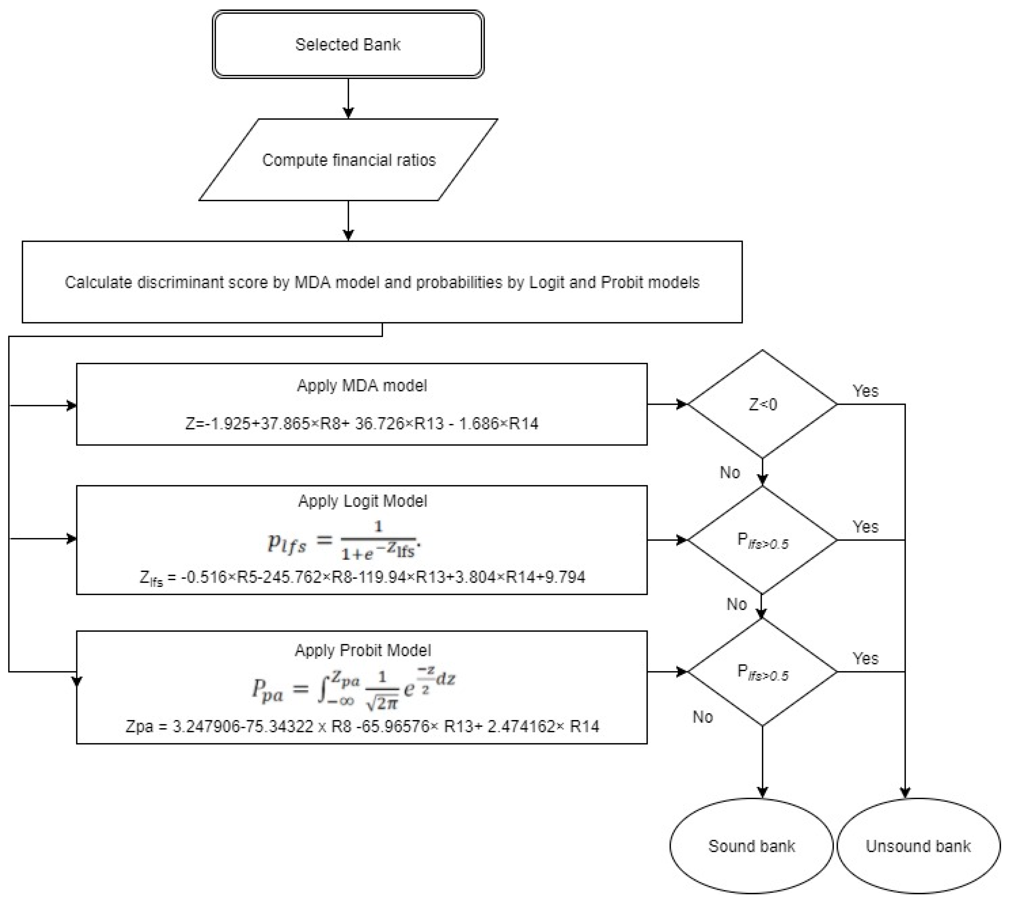
Table 1.
Summary of Prior Studies on Bank Bankruptcy/Failure Prediction
| Literature | Sample | Method | Predictive ability, % | Type 1, % | Type 2, % |
| Meyer and Pifer (1970) | USA banks | MDA | 80.00 | 3 | 0 |
| Sinkey (1975) | USA banks | MDA | 77.67 | 13.59 | 22.3 |
| Martin (1977) | USA banks | Logit regression | 82.00 | n/a | n/a |
| Bovenzi (1983) | USA banks | Probit analysis | 91.00 | n/a | n/a |
| West (1985) | USA banks | Logit analysis, Factor analysis | 90.50 | n/a | n/a |
| Espahbodi (1991) | USA banks | Logit analysis | 86.30 | n/a | n/a |
| Discriminant models | 84.24 | n/a | n/a | ||
| Estrella, Park and Perisitiani (2000) | USA banks | Logit regression | 80.00 | 4.8 | 7.3 |
| Kuznetsov (2003) | Russia banks | Logit model | 87.00 | 68.2 | 2.6 |
| Rahman et.al (2004) | Indonesia, South Korea and Thailand banks | Logit model | 85.00 | 11 | 20 |
| Canbas, Cabuk and Kilic (2005) | Turkey banks | MDA, Logit and Probit analysi, PCA and IEWS | 87.50 - 90.00 |
15 - 25 |
5 -30 |
| Ioannidis, Pasiouras and Zopounidis (2010) | 78 countries | MDA, UTADIS, ANN, k-NN, OLR and Stacked model | 68.00 - 95.00 |
n/a | n/a |
| Betz et. al (2014) | Europe banks | Logit model | 57.00 - 60.00 | n/a | n/a |
| Affes and Hentati-Caffel (2016) | USA banks | Logit | 98.82 | 33.33 | 0.6 |
| Canonical discriminant analysis | 98.59 | 46.67 | 0.6 | ||
| Kimmel, Thornton Jr. and Bennett (2016) | USA banks | Logit, MDA, PHM, Trait and LOESS | 96.00 | n/a | n/a |
| Othman (2018) | Malaysia banks | MDA, Logit analysis, Probit analysis Factor analysis and Integrated model |
73.00-93.00 | n/a | n/a |
| Filippopoulou, C., Galariotis, E., & Spyrou, S. (2020). | Euro Zone Banks | Logit | 94.17, 95.00 | 21.67, 11.67 | 2.67, 3.67 |
| Boos et al. (2023) | Swiss Banks | Logit and Probit | n/a | n/a | n/a |
| Barajas, Krakovich, and López-Iturriaga (2023) | Russian banks | Logit, Survival Analysis | 65.15-66.91 | 75.00 | 58.00 |
| Ekinci and Sen, (2023) | US Banks | Logit | TPR 99.51 | 0.49 | 18.64 |
| Machine learning techniques | 99.09 – 99.72 | 0.28 – 0.91 | 20.34 – 33.90 |
Table 2.
Test of Equality of Group Means 2008 - 2012
| Variable | Sound banks | Unsound banks | Wilks' Lambda |
F test (p-value) |
T test (p-value) |
Mann–Whitney U-test (sig.) | ||
| Mean | Std. Dev. | Mean | Std. Dev. | |||||
| R1 | 0.249 | 0.247 | 0.070 | 0.279 | 0.893 | 0.786 (0.261) | 2.632* (0.005) | 410 (0.554) |
| R2 | 0.196 | 0.214 | 0.033 | 0.279 | 0.899 | 0.589 (0.080) | 2.546* (0.007) | 445 (0.941) |
| R3 | 0.240 | 0.247 | 0.074 | 0.195 | 0.875 | 1.597 (0.107) | 2.884* (0.003) | 390.5 (0.379) |
| R4 | 0.909 | 2.060 | 0.122 | 0.192 | 0.930 | 115.61* (0.000) | 2.083* (0.023) | 429 (0.756) |
| R5 | 5.489 | 2.657 | 4.908 | 2.775 | 0.988 | 0.917 (0.408) | 0.828 (0.206) | 339 (0.101) |
| R6 | 0.045 | 0.037 | 0.218 | 0.226 | 0.773 | 0.027* (0.000) | -4.124* (0.000) | 250* (0.003) |
| R7 | 0.222 | 0.192 | 0.905 | 1.482 | 0.902 | 0.017* (0.000) | -2.505* (0.009) | 325 (0.065) |
| R8 | 0.016 | 0.015 | 0.010 | 0.008 | 0.943 | 3.725* (0.000) | 1.878* (0.034) | 292.5* (0.019) |
| R9 | 0.008 | 0.014 | -0.056 | 0.368 | 0.985 | 0.001* (0.000) | 0.947 (0.176) | 313* (0.043) |
| R10 | 0.047 | 0.114 | 0.495 | 1.385 | 0.949 | 0.007* (0.000) | -1.767* (0.044) | 432 (0.790) |
| R11 | 0.061 | 0.029 | 0.032 | 0.345 | 0.996 | 0.007* (0.000) | 0.457 (0.326) | 410 (0.554) |
| R12З | 0.057 | 0.032 | 0.028 | 0.026 | 0.788 | 1.495 (0.142) | 3.947* (0.000) | 191* (0.000) |
| R13 | 0.047 | 0.029 | 0.014 | 0.024 | 0.714 | 1.444 (0.164) | 4.823* (0.000) | 150* (0.000) |
| R14 | -0.334 | 0.631 | -0.039 | 0.365 | 0.922 | 2.985* (0.002) | -2.217* (0.016) | 278* (0.011) |
| R15 | 1.253 | 1.030 | 1.322 | 0.793 | 0.999 | 1.688 (0.082) | -0.289 (0.387) | 397 (0.433) |
Table 3.
Eigenvalues
| Function | Eigenvalue | % of Variance | Cumulative % | Canonical Correlation |
| 1 | 0.958 | 100.0 | 100.0 | 0.700 |
a. First 1 canonical discriminant functions were used in the analysis.
Table 4.
Wilks' lambda
| Test of Function(s) | Wilks' Lambda | Chi-square | df | Sig. |
| 1 | 0.511 | 37.976 | 3 | 0.000 |
Table 5.
Standardized Canonical Discriminant Function Coefficients
| Standardized Canonical Discriminant Function Coefficients | Function |
| R8 | 0.443 |
| R13 | 0.974 |
| R14 | -0.869 |
Table 7.
Structure Matrix
| Function | |
| R8 | 37.865 |
| R13 | 36.726 |
| R14 | -1.686 |
| (Constant) | -1.925 |
Unstandardized coefficients
Table 9.
Out sample Classification Results
| Default | Predicted Group Membership | Total | ||
| Sound | Unsound | |||
| Count | Sound | 9 | 3 | 12 |
| Unsound | 1 | 11 | 12 | |
| Accuracy % | Sound | 75.0 | 25.0 | 100.0 |
| Unsound | 8.3 | 91.7 | 100.0 | |
83.3% of original grouped cases correctly classified
Table 11.
Omnibus Tests of Model Coefficients
| Chi-aquare | df | Sig | ||
| Step | Step | 46,861 | 4 | 0.000 |
| 1 | Block | 46,861 | 4 | 0.000 |
| Model | 46,861 | 4 | 0.000 |
Table 12.
Model Summary
| Step | -2 Log likelihood | Cox & Snell R Square | Nagelkerke R Square |
| 1 | 36.316a | 0.542 | 0.723 |
a. Estimation terminated at iteration number 6 because parameter estimates changed by less than 0.001
Table 14.
Out Sample Classification Table
| Observed | Predicted | ||
| Sound | Unsound | Percentage Correct | |
| Sound | 10 | 2 | 83.3 |
| Unsound | 1 | 11 | 91.7 |
| Overall Percentage | 87.5 | ||
Table 15.
Table of Classification of Logit Model Errors
| Type of Error |
Number correct |
% correct |
% error |
Total observations |
| Type I | 11 | 91.7 | 8.3 | 12 |
| Type II | 10 | 83.3 | 16.7 | 12 |
| Total | 21 | 87.5 | 12.5 | 24 |
Table 16.
Test Statistics for Probit Model
| Dependent Variable: STATUS | ||||
| Method: ML - Binary Probit (Quadratic hill climbing) | ||||
| Date: 06/29/17 Time: 09:38 | ||||
| Sample: 1 60 | ||||
| Included observations: 60 | ||||
| Convergence achieved after 6 iterations | ||||
| Covariance matrix computed using second derivatives | ||||
| Variable | Coefficient | Std. Error | z-Statistic | Prob. |
| Type I | 11 | 91.7 | 8.3 | 12 |
| C | 3.247906 | 0.963978 | 3.369273 | 0.0008 |
| R8 | -75.34322 | 33.15429 | -2.272503 | 0.0231 |
| R13 | -65.96576 | 21.40151 | -3.082294 | 0.0021 |
| R14 | 2.474162 | 0.869999 | 2.843868 | 0.0045 |
| McFadden R-squared | 0.528058 | Mean dependent var | 0.5 | |
| S.D. dependent var | 0.504219 | S.E. of regression | 0.345668 | |
| Akaike info criterion | 0.787584 | Sum squared resid | 6.691236 | |
| Schwarz criterion | 0.927207 | Log likelihood | -19.62751 | |
| Hannan-Quinn criter. | 0.842198 | Deviance | 39.25503 | |
| Restr. Deviance | 83.17766 | Restr. log likelihood | -41.58883 | |
| LR statistic | 43.92263 | Avg. log likelihood | -0.327125 | |
| Prob(LR statistic) | 0 | |||
| Obs with Dep=0 | 30 | Total obs | 60 | |
| Obs with Dep=1 | 30 | |||
Zpa equation takes the following form:
Table 17.
Classification of the Probit Model Errors
| Type of Error |
Number correct |
% correct |
% error |
Total observations |
| Type I | 11 | 91.7 | 8.3 | 12 |
| Type II | 9 | 75.0 | 25.0 | 12 |
| Total | 20 | 83.3 | 16.7 | 24 |
Table 18.
Cut-off Points of the MDA, Logit and Probit Models
| Percen-tile | MDA | Logit | Probit | ||||||
| Predictive accuracy | Type I | Type II | Predictive accuracy | Type I | Type II | Predictive accuracy | Type I | Type II | |
| 25 | 75.00% | 50.00% | 0.00% | 75.00% | 0.00% | 50.00% | 79.17% | 0.00% | 41.67% |
| 30 | 79..17% | 41..67% | 0.00% | 79.17% | 0.00% | 41.67% | 83.33% | 0.00% | 33.33% |
| 35 | 87.50% | 25.00% | 0.00% | 87.50% | 0.00% | 25.00% | 83.33% | 0.00% | 33.33% |
| 40 | 83.33% | 25.00% | 8.33% | 91.67% | 0.00% | 16.67% | 87.50% | 0.00% | 25.00% |
| 50 | 87.50% | 16.67% | 8.33% | 87.50% | 8.33% | 16.67% | 87.50% | 8.33% | 16.67% |
| 55 | 87.50% | 8.33% | 16.67% | 91.67% | 8.33% | 8.33% | 91.67% | 8.33% | 8.33% |
| 60 | 83.33% | 8.33% | 25.00% | 91.67% | 16.67% | 0.00% | 95.83% | 8.33% | 0.00% |
| 65 | 79.17% | 8.33% | 33.33% | 87.50% | 25.00% | 0.00% | 83.33% | 33.33% | 0.00% |
| 70 | 79.17% | 0.00% | 41.67% | 79.17% | 41.67% | 0.00% | 83.33% | 33.33% | 0.00% |
| 75 | 75.00% | 0.00% | 50.00% | 75.00% | 50.00% | 0.00% | 75.00% | 50.00% | 0.00% |
Table 19.
Table of Classification of Integrated Bank Unsoundness Prediction Model Errors, 2013 – 2014
Table 19.
Table of Classification of Integrated Bank Unsoundness Prediction Model Errors, 2013 – 2014
|
Type of Error |
Number correct |
% correct |
% error |
Total observations |
| Type I | 12 | 100.0 | 0.0 | 12 |
| Type II | 9 | 75.0 | 25.0 | 12 |
| Total | 21 | 87.5 | 12.5 | 24 |
Table 20.
Comparative Quality Assessment of Models
|
MDA model |
Logit model |
Probit model |
Integrated model |
|
| Failed banks correctly predicted | 11 | 11 | 11 | 12 |
| Non-failed banks correctly predicted | 9 | 10 | 9 | 9 |
| Type I error | 1 | 1 | 1 | 0 |
| Type II error | 3 | 2 | 3 | 3 |
| Incorrectly predicted in total | 4 | 3 | 4 | 3 |
| Correctly predicted in total | 20 | 21 | 20 | 21 |
| % of failed banks correctly predicted | 91.7 | 91.7 | 91.7 | 100 |
| % of non-failed banks correctly predicted | 75.0 | 83.3 | 75.0 | 75.0 |
| % of total incorrectly predicted | 16.7 | 12.5 | 16.7 | 12.5 |
| %Type I error | 8.3 | 8.3 | 8.3 | 0 |
| %Type II error | 25.0 | 16.7 | 25.0 | 25.0 |
| % of total correctly predicted | 83.3 | 87.5 | 83.3 | 87.5 |
Disclaimer/Publisher’s Note: The statements, opinions and data contained in all publications are solely those of the individual author(s) and contributor(s) and not of MDPI and/or the editor(s). MDPI and/or the editor(s) disclaim responsibility for any injury to people or property resulting from any ideas, methods, instructions or products referred to in the content. |
© 2025 by the authors. Licensee MDPI, Basel, Switzerland. This article is an open access article distributed under the terms and conditions of the Creative Commons Attribution (CC BY) license (http://creativecommons.org/licenses/by/4.0/).
Copyright: This open access article is published under a Creative Commons CC BY 4.0 license, which permit the free download, distribution, and reuse, provided that the author and preprint are cited in any reuse.


