
Submitted:
17 October 2025
Posted:
21 October 2025
You are already at the latest version
Abstract
We employ a two-dimensional fluid simulation approach to study the nonlinear turbulent dynamics of internal gravity waves (IGWs) in the weakly ionized Earth’s ionospheric F-layer with the effects of Pedersen conductivity. We observe that the presence of Pedersen conductivity leads to the formation of intermediate-scale structures in the velocity potential, along with the development of small-scale density fluctuations. The characteristic turbulent energy spectrum exhibits a non-Kolmogorov scaling of k−2.40 in the presence of Pedersen conductivity, while a Kolmogorov-like k−5/3 scaling is observed when it is absent, where k denotes the wave number. Due to energy loss caused by Pedersen conductivity, the wave’s amplitude reduces gradually with time. The cross-field diffusion coefficient related to the velocity potential also reduces as Pedersen conductivity increases. The results in the F-layer are compared with those in the literature, e.g., J. Geophys. Res., 113, D06108 (2008), where the Ampére force and hence the Pedersen conductivity effect were ignored compared to the pressure gradient and gravity forces, as relevant in the Earth’s D-layer.
Keywords:
internal gravity wave
; fluid turbulence
; solitary vortex
; Earth’s ionosphere
1. Introduction
Acoustic-gravity waves (AGWs) play crucial roles in characterizing ionospheric plasma dynamics. They are essential for accurately predicting atmospheric behaviors under varying meteorological conditions in the Earth’s atmosphere, the stratified layers of the solar atmosphere, and the magnetospheric environments of other planets [1,2,3,4,5,6]. A low-frequency branch of AGWs is typically known as internal gravity waves (IGWs), which have frequencies in the range and wavelengths of approximately 10 km. IGWs propagate only in stable stratified fluids, when the typical Brunt–Väisälä frequency is positive. They play a vital role in transporting wave energy to charged particles in the Earth’s atmosphere and ionosphere. The nonlinear evolution of these waves and their interactions with fluid density perturbations are fundamental to both geophysical and applied research in atmospheric convection and the generation of atmospheric turbulence [7].
Nonlinear interactions between finite-amplitude AGWs in the Earth’s atmosphere lead to both resonant and nonresonant energy transfer between high- and low-frequency components of the wave spectrum, with resonant processes playing a significant role in rotating atmospheric conditions [8]. Analytical studies [9] exploring nonlinear couplings among acoustic-gravity modes with different wavelengths suggest the development of vortical structures. Gardner [10] described the vertical wavenumber spectrum as a scale-independent diffusivity that accounts for damping due to molecular viscosity, turbulence, and off-resonant wave-wave interactions. Similarly, a physically based gravity wave source spectrum parameterization for convection was implemented in a Global Circulation Model by Beres et al. [11]. Shaikh et al. [7] investigated the turbulent behavior of two-dimensional nonlinearly interacting IGWs and showed that the governing nonlinear equations for vorticity and density fluctuations in a nonuniform fluid lead to a dual cascade, resulting in an energy spectrum indicative of Kolmogorov-type turbulence.
The role of charged particles in the ionosphere and their effect on nonlinear solitary vortices associated with planetary Rossby waves was first systematically explored by Kaladze and Tsamalashvili [12], and later expanded upon in the works of Kaladze [13,14] and Kaladze et al. [15]. A detailed analysis of how these charged particles affect the linear and nonlinear propagation characteristics of acoustic gravity waves in the weakly ionized and electrically conductive D, E, and F layers of the ionosphere while accounting for the Coriolis force was provided in [16]. The latter proposed an extended two-dimensional model for the evolution of IGW-driven solitary vortices, including the effect of Pedersen conductivity, and concluded that Pedersen conductivity dissipates the wave energy due to the Ohm losses. The work also discussed how the Hall conductivity and the Coriolis force due to rotating fluids are irrelevant, but Pedersen conductivity can not be in the ionospheric F-layer. The theory was recently advanced in [17] employing analytical and numerical approaches to explore different forms of dipolar vortex structures and their time-dependent evolution, demonstrating how Pedersen conductivity and system nonlinearities influence their dynamics.
In this work, we aim to present a detailed numerical investigation of the turbulent properties of nonlinearly interacting IGWs in the ionospheric F-layer by the effects of Pedersen conductivity, thereby advancing further the nonlinear theory of IGW-driven solitary vortices as in Refs. [7,16,17]. Although Shaikh et al. [7] presented a similar study without the effects of Pedersen conductivity, the results may be relevant in the ionospheric D-layer. Here, we consider the Earth’s F-layer to analyze the turbulent spectrum resulting from dual cascading, along with the associated fluid diffusion influenced by large-scale structures, and compare the results without the effect of Pedersen conductivity, such as those in the D-layer or Ref. [7].
2. Basic Equations
The nonlinear dynamics of solitary vortices driven by IGWs or low-frequency AGWs in stable stratified ionospheric incompressible fluids can be described by the following coupled equations [16].
where , is the velocity potential (stream function), is the normalized fluid density perturbation, H is the fluid density scale height, is the Brunt–Väisälä frequency with g denoting the constant gravitational acceleration, denotes the Jacobian of two functions a and b, is the constant background fluid density, is the constant geomagnetic field, and is the Pedersen conductivity. In the absence of the latter, Eqs. (1) and (2) reduce to those in Ref. [18].
Before, proceeding to study Eqs. (1) and (2) numerically for the turbulent wave dynamics of IGW-driven solitary vortices, we review some results as in Ref. [16], namely, the energy conservation, an estimation for the Pedersen conductivity, and the dispersion relation and the damping or growth rate of instability. From Eqs. (1) and (2), it is straightforward to obtain the following energy conservation equation [16].
where E is the total energy, given by,
Since the integral on the right-hand side of Eq. (3) is positive definite, the negative sign before it indicates that the wave energy dissipates with time by the influence of the Pedersen conductivity.
Typical forces influencing IGW dynamics include the pressure gradient force, gravity, the Coriolis force, and the force. The current can be associated with parallel, perpendicular (Pedersen), or Hall conductivity. Pressure gradient and gravity are prerequisites for AGWs. The Coriolis and forces are not always relevant in all three ionospheric layers (D, E, F). For details, see Ref. [16]. In the D-layer, the force (and, thus, Pedersen conductivity) is negligibly small compared to the Coriolis and other forces. In the E layer, this force matters mainly due to the Hall current. In contrast, in the F layer, the force, driven by Pedersen conductivity, dominates, even over the Coriolis force. Therefore, in the model equations (1) and (2), the relevant forces are the pressure gradient, (from the Pedersen current), and gravity.
In what follows, we estimate the ratio , associated with the Pedersen conductivity . As in Refs. [16,19], the conditions and hold good in the F-layer, where and are, respectively, the electron and ion-cyclotron frequencies and with , , and denoting, respectively, the electron-ion, electron-neutral, and ion-neutral collision frequencies. Under these conditions, the Pedersen conductivity can be approximated as: , where is the parallel conductivity. Using the typical F-layer values [16], , , , , , and , we estimate, . Next, we consider the linear analysis to obtain the dispersion relation and the damping rate associated with the Pedersen conductivity of Eqs. (8) and (9). Assuming the perturbations to vary as plane waves of the form, , where is the wave frequency and and are, respectively, the wave vector components along the x- and z-directions, and letting , where , we obtain the following dispersion relation [16]
and the damping rate, given by,
where . From Eqs. (5) and (6), it is evident that the IGW mode has the characteristics similar to low-frequency ion-acoustic waves in plasmas, and the damping indeed occurs due to Pedersen conductivity and the damping rate is of the order of the ratio , the key parameter in the model equations.
To begin the simulation study in Sec. Section 3, it is imperative to make Eqs. (1) and (2) dimensionless by redefining the variables as follows:
where and denote, respectively, the characteristic length and time scales. The dimensionless parameters , , and , respectively, correspond to the Jacobian nonlinearities, the normalized Pedersen conductivity, and the normalized frequency. Thus, Eqs. (1) and (2) reduce to
3. Simulation Results and Discussion
We numerically study the nonlinear interactions of the large-scale velocity field potential (stream function) and small-scale density perturbations, as described by Eqs. (8) and (9). To this end, we develop a two-dimensional spectral code for the numerical integration of these equations [7,20]. The initial conditions consist of isotropic fluctuations with no imposed mean fields constructed using random amplitudes and phases in Fourier space. Spatial discretization is achieved in our simulations through a discrete Fourier representation of the turbulent fields. Numerical stability is maintained by applying proper dealiasing techniques to eliminate spurious Fourier modes. We use the fourth-order Runge-Kutta (RK4) scheme to solve the equations over time, with a time step, . The computational domain contains modes in two dimensions. Furthermore, , so that , and depending on the magnetic field strength in the F-layer. Also, we take and throughout the simulation.
We note that the turbulent dynamics of IGWs, described by Eqs. (8) and (9) with , are known in the literature [7] and may apply to the ionospheric D-layer. We reproduce the results for to compare with those in the F-layer. As observed earlier in Ref. [7] for , the perturbed velocity potential forms large-scale structures. In contrast, density fluctuations cascade to smaller spatial scales. The coexistence of both large- and small-scale structures is the key feature of two-dimensional turbulent systems. Specifically, two-dimensional hydrodynamic turbulence in an incompressible fluid conserves both energy and mean-squared vorticity. Under external forcing, these conserved quantities exhibit a dual cascade. The forward cascade generates small-scale structures, while the inverse cascade leads to large-scale structures. Such dynamics typically appear in driven turbulence simulations, as in the present work. In these, specific modes are randomly excited in spectral space, redistributing energy and preserving physical invariants in k-space [7]. Similar features appear for (see left panels of Figure 1 and Figure 2). In the F-layer (), the initially randomly propagating IGWs interact and generate large-scale velocity potential structures in the early phase (see right panels of Figure 1 at different times). As the system evolves, these structures break into intermediate-scale features due to the Pedersen conductivity. Meanwhile, density perturbations develop into smaller-scale structures (see right panels of Figure 2 at different times). Increasing values of the parameter also cause a faster decay of wave amplitudes, emphasizing the damping effect on the vortex dynamics.
During the decay of wave turbulence, energy in large-scale eddies cascades down to smaller scales, establishing a statistically steady inertial regime characterized by the forward transfer of one of the system’s invariants. Decaying turbulence frequently results in the emergence of coherent structure as it relaxes, which causes nonlinear interactions to become inefficient once they saturate. IGWs appear to exhibit turbulence similar to two-dimensional hydrodynamic turbulence, where density and velocity potential fluctuations correspond to fluid energy and vorticity, respectively [7]. Subplot (a) of Figure 3 illustrates the evolution of energy associated with the density and potential field modes (The case of ). Once the nonlinear interactions saturate, the turbulent energy stops growing and remains almost constant throughout the simulations. However, after nonlinear interactions saturate, the transfer of energy among turbulent modes in spectral space becomes inefficient, and the energy transfer rate becomes insignificant. Higher k-values dominate the energy, so dissipation by Pedersen conductivity is expected to dissipate the turbulent energy effectively. In contrast, subplot (b) of Figure 3 illustrates a significant decay of the turbulent energy. This behavior is primarily driven by dissipation associated with Pedersen conductivity (). As a result, higher Pedersen conductivity leads to a more rapid decay of turbulent energy.
The inertial range spectrum should contain characteristic features of strongly anisotropic turbulent flows. As such, the energy spectrum resulting from IGW turbulence under the effect of Pedersen conductivity may differ from the classical Kolmogorov form. To examine the spectral characteristics of IGW turbulence, the inertial range energy spectrum is presented in Figure 4. The inertial range energy spectrum exhibits a Kolmogorov-like scaling when Pedersen conductivity is absent [, Subplot (a)]. In the F-layer, when is increased to , the spectrum becomes significantly steeper, with a spectral index close to [Subplot (b)]. This index deviates from the usual Kolmogorov-like () scaling, indicating that, in the F-layer, the effect of Pedersen conductivity leads to weaker turbulence compared to the D-layer or Ref. [7].
Finally, we estimate the turbulent transport coefficient arising from the self-consistent dynamics of small- and large-scale turbulent fluctuations. An effective electron diffusion coefficient due to momentum transfer can be expressed as
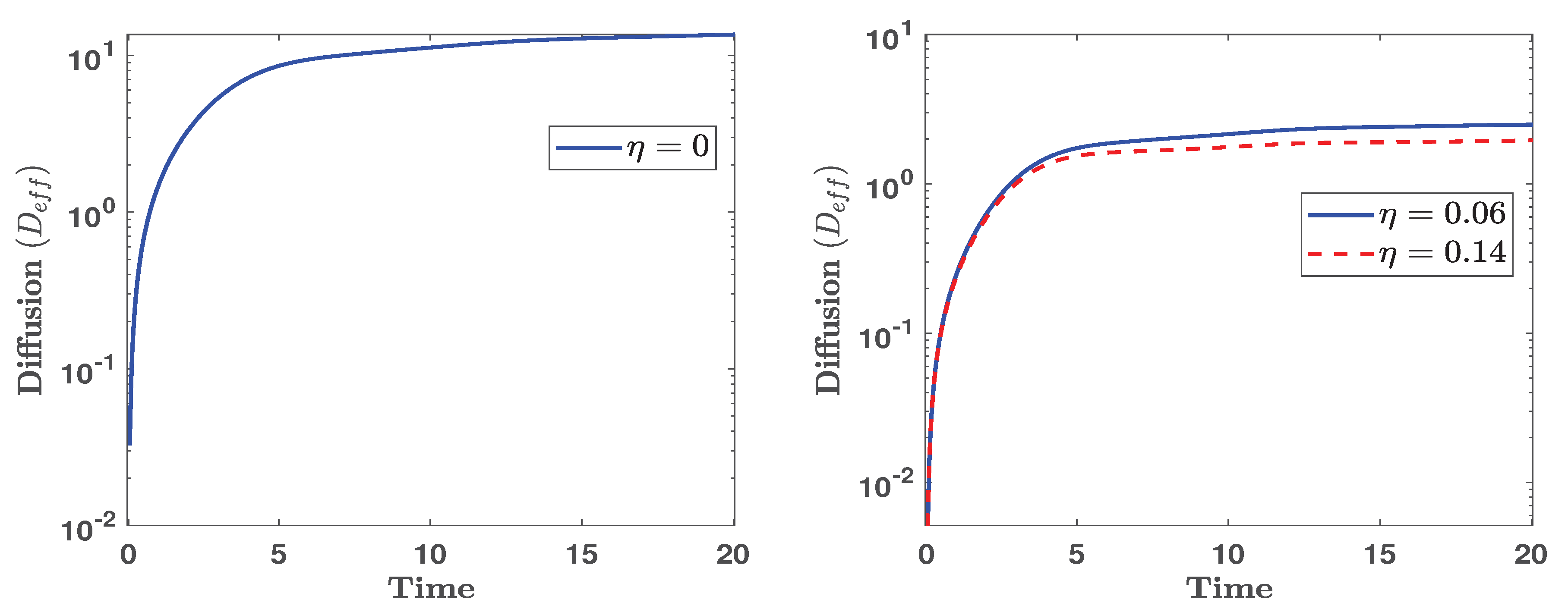
where is the fluid velocity, the angular bracket denotes spatial averaging, and ensemble averages are normalized to unit mass [7]. In our simulations, we compute the effective diffusion coefficient, , from both the velocity field and its fluctuations to quantify turbulent transport associated with large-scale flows in the F-layer, for different values of Pedersen conductivity. As previously noted in Ref. [7], and as also demonstrated in our simulations [See Figure 5, subplot (a)], the effective cross-field transport remains low during the initial phase due to the Gaussian nature of field perturbations. As turbulence increases and large-scale structures begin to form, the diffusion coefficient grows rapidly, indicating stronger transport. Moreover, when the system reaches a steady state, the nonlinearly coupled modes form stationary structures, and eventually becomes saturated. The primary cause of the enhanced cross-field transport is the emergence of large-scale structures within turbulence dominated by IGWs. We also examine the fluid transport by considering the influence of the Pedersen conductivity. The effective diffusion coefficient, , is derived from the cross-correlation of the particle drift velocity, as described by equation (10). As shown in Figure 5 (b), gradually levels off as the system transits into a steady-state regime with reduced energy transfer by the influence of .
4. Conclusion
We have investigated the turbulent dynamics of IGW-driven vortex turbulence in the conductive ionosphere, focusing on the F-layer, where the Pedersen current plays a dominant role over the parallel and Hall currents, and compared the results with those without this effect, e.g., relevant in the D-layer. Our analysis shows that, in contrast to the D-layer or where the effect of the Pedersen current is insignificant, the large-scale perturbed velocity potential and small-scale density fluctuations in the F-layer exhibit a non-Kolmogorov-like energy spectrum. We also observe that the formation of intermediate-scale structures in the F-layer can lead to significantly lower cross-field diffusion than that in the D-layer. The system’s energy loss occurs due to magnetic viscosity, influenced by Pedersen conductivity in the F-region. This energy dissipation can lead to a reduction in the vortex structure [17].
To conclude, the turbulent dynamics of IGWs could help infer atmospheric and space weather conditions, understand the coupling of magnetospheric and ionospheric perturbations, and predict disruptions to radio signals.
Author Contributions
Conceptualization, S.D.A. and A.P.M.; methodology, S.D.A. and A.P.M.; software, S.D.A.; validation, S.D.A. and A.P.M.; formal analysis, S.D.A. and A.P.M.; investigation, S.D.A. and A.P.M.; writing—original draft preparation, S.D.A; writing—review and editing, A.P.M; visualization, S.D.A.; supervision, A.P.M. All authors have read and agreed to the published version of the manuscript.
Funding
This research received no external funding.
Data Availability Statement
No new data were created or analyzed in this study. Data sharing is not applicable to this article.
Acknowledgments
This work was dedicated to Prof. Lennart Stenflo on the occasion of his 85th birthday. S. Das Adhikary thanks the University Grants Commission (UGC), Government of India, for support through a junior research fellowship (JRF) with NTA reference no. 211610078837. A. P. Misra gratefully acknowledges continued encouragement and support from Prof. Lennart Stenflo, who instilled in him a spirit of research, especially in the field of Atmospheric Fluid Dynamics.
Conflicts of Interest
The authors declare no conflicts of interest.
Abbreviations
The following abbreviations are used in this manuscript:
| AGW | Acoustic Gravity Wave |
| IGW | Internal Gravity Wave |
References
- Stenflo, L. Acoustic solitary vortices. The Physics of Fluids 1987, 30, 3297–3299. [Google Scholar] [CrossRef]
- Yeh, K.C.; Liu, C.H. Acoustic-gravity waves in the upper atmosphere. Reviews of Geophysics 1974, 12, 193–216. [Google Scholar] [CrossRef]
- Jovanović, D.; Stenflo, L.; Shukla, P.K. Acoustic-gravity nonlinear structures. Nonlinear Processes in Geophysics 2002, 9, 333–339. [Google Scholar] [CrossRef]
- Fritts, D.C.; Alexander, M.J. Gravity wave dynamics and effects in the middle atmosphere. Reviews of Geophysics 2003, 41, 1003. [Google Scholar] [CrossRef]
- Hines, C.O. INTERNAL ATMOSPHERIC GRAVITY WAVES AT IONOSPHERIC HEIGHTS. Canadian Journal of Physics 1960, 38, 1441–1481. [Google Scholar] [CrossRef]
- Hooke, W. Ionospheric irregularities produced by internal atmospheric gravity waves. Journal of Atmospheric and Terrestrial Physics 1968, 30, 795–823. [Google Scholar] [CrossRef]
- Shaikh, D.; Shukla, P.K.; Stenflo, L. Spectral properties of acoustic gravity wave turbulence. Journal of Geophysical Research: Atmospheres 2008, 113, D06108. [Google Scholar] [CrossRef]
- Axelsson, P.; Larsson, J.; Stenflo, L. Nonlinear interaction between acoustic gravity waves in a rotating atmosphere. Nonlinear Processes in Geophysics 1996, 3, 216–220. [Google Scholar] [CrossRef]
- Stenflo, L. Acoustic gravity vortex chains. Physics Letters A 1994, 186, 133–134. [Google Scholar] [CrossRef]
- Gardner, C.S. Diffusive filtering theory of gravity wave spectra in the atmosphere. Journal of Geophysical Research: Atmospheres 1994, 99, 20601–20622. [Google Scholar] [CrossRef]
- Beres, J.H.; Garcia, R.R.; Boville, B.A.; Sassi, F. Implementation of a gravity wave source spectrum parameterization dependent on the properties of convection in the Whole Atmosphere Community Climate Model (WACCM). Journal of Geophysical Research: Atmospheres 2005, 110, D10108. [Google Scholar] [CrossRef]
- Kaladze, T.; Tsamalashvili, L. Solitary dipole vortices in the Earth’s ionosphere. Physics Letters A 1997, 232, 269–274. [Google Scholar] [CrossRef]
- Kaladze, T.D. Nonlinear vortical structures in the Earth’s ionosphere. Physica Scripta 1998, 1998, 153. [Google Scholar] [CrossRef]
- Kaladze, T. Magnetized Rossby waves in the Earth’s ionosphere. Plasma Physics Reports 1999, 25. [Google Scholar]
- Kaladze, T.D.; Aburjania, G.D.; Kharshiladze, O.A.; Horton, W.; Kim, Y.H. Theory of magnetized Rossby waves in the ionospheric E layer. Journal of Geophysical Research: Space Physics 2004, 109, A05302. [Google Scholar] [CrossRef]
- Kaladze, T.; Pokhotelov, O.; Shah, H.; Khan, M.; Stenflo, L. Acoustic-gravity waves in the Earth’s ionosphere. Journal of Atmospheric and Solar-Terrestrial Physics 2008, 70, 1607–1616. [Google Scholar] [CrossRef]
- Kaladze, T.; Misra, A.; Roy, A.; Chatterjee, D. Nonlinear evolution of internal gravity waves in the Earth’s ionosphere: Analytical and numerical approach. Advances in Space Research 2022, 69, 3374–3385. [Google Scholar] [CrossRef]
- Stenflo, L. Nonlinear equations for acoustic gravity waves. Physics Letters A 1996, 222, 378–380. [Google Scholar] [CrossRef]
- Kaladze, T.D.; Özcan, O.; Yeşil, A.; Tsamalashvili, L.V.; Kaladze, D.T.; Inc, M.; Sağir, S.; Kurt, K. Shear flow-driven magnetized Rossby wave dynamics in the Earth’s ionosphere. Zeitschrift für angewandte Mathematik und Physik 2021, 72, 130. [Google Scholar] [CrossRef]
- Shaikh, D.; Zank, G.P. The Transition to Incompressibility from Compressible Magnetohydroynamic Turbulence. The Astrophysical Journal 2006, 640, L195. [Google Scholar] [CrossRef]
Figure 1.
Evolution of the potential function () at times , , , and . The left panels illustrate the emergence of large-scale structures with (e.g., ionospheric D-layer) due to an inverse cascade process. The right panels highlight the development of intermediate-scale eddies with (e.g., ionospheric F-layer).
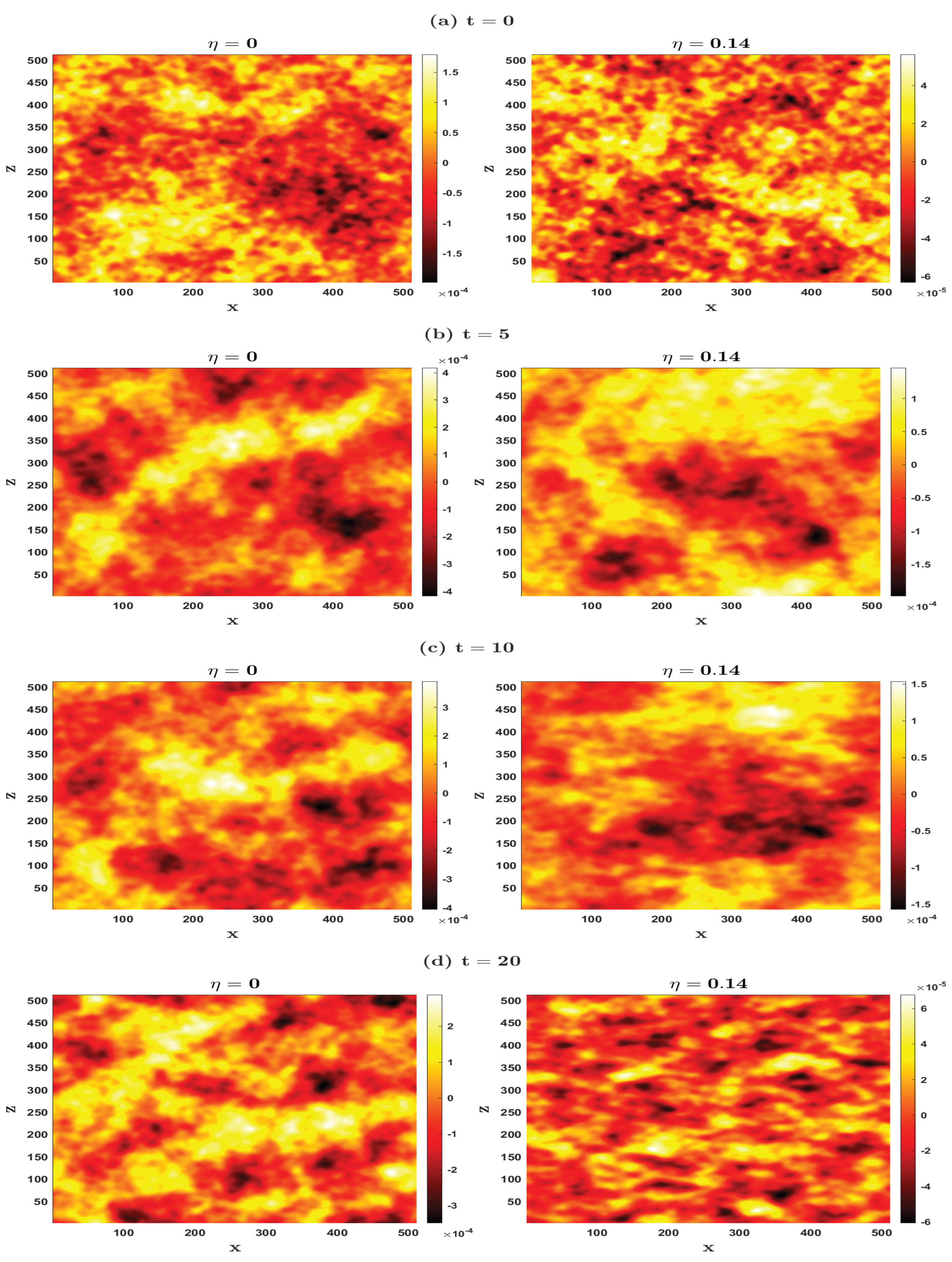
Figure 2.
Evolution of the density fluctuations () at times , , , and . The left panels illustrate the emergence of small-scale structures with (e.g., ionospheric D-layer) due to a forward cascade process. The right panels highlight the development of small-scale eddies with (e.g., ionospheric F-layer), resulting from the forward cascade of density fluctuations.
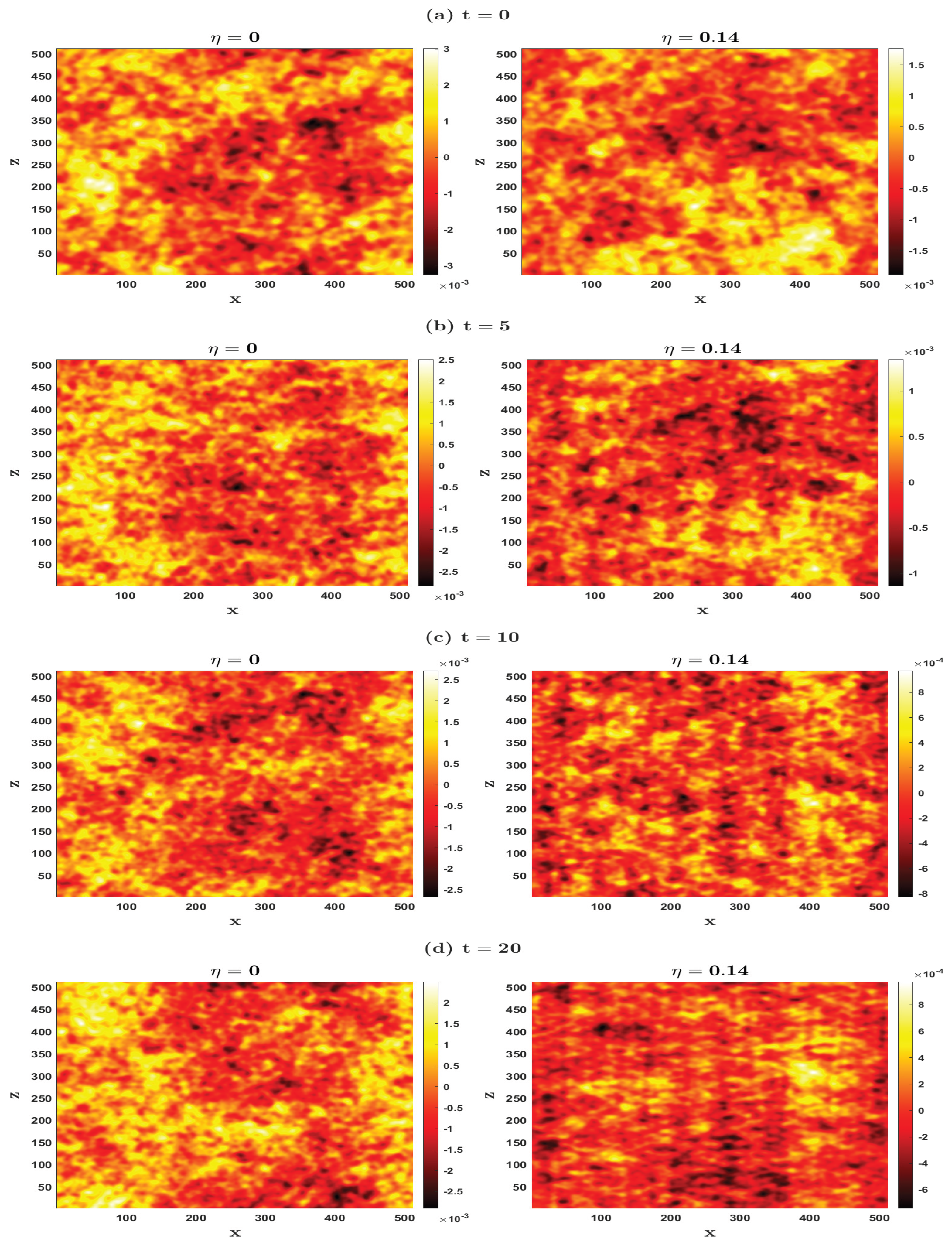
Figure 3.
The evolution of the total energy is shown. Subplot (a) is for , where the energy increases until nonlinear interactions get saturated. Subplot (b) is for in which a decay in energy is observed for different values of : and . The decay is faster the larger are the values of .
Figure 3.
The evolution of the total energy is shown. Subplot (a) is for , where the energy increases until nonlinear interactions get saturated. Subplot (b) is for in which a decay in energy is observed for different values of : and . The decay is faster the larger are the values of .
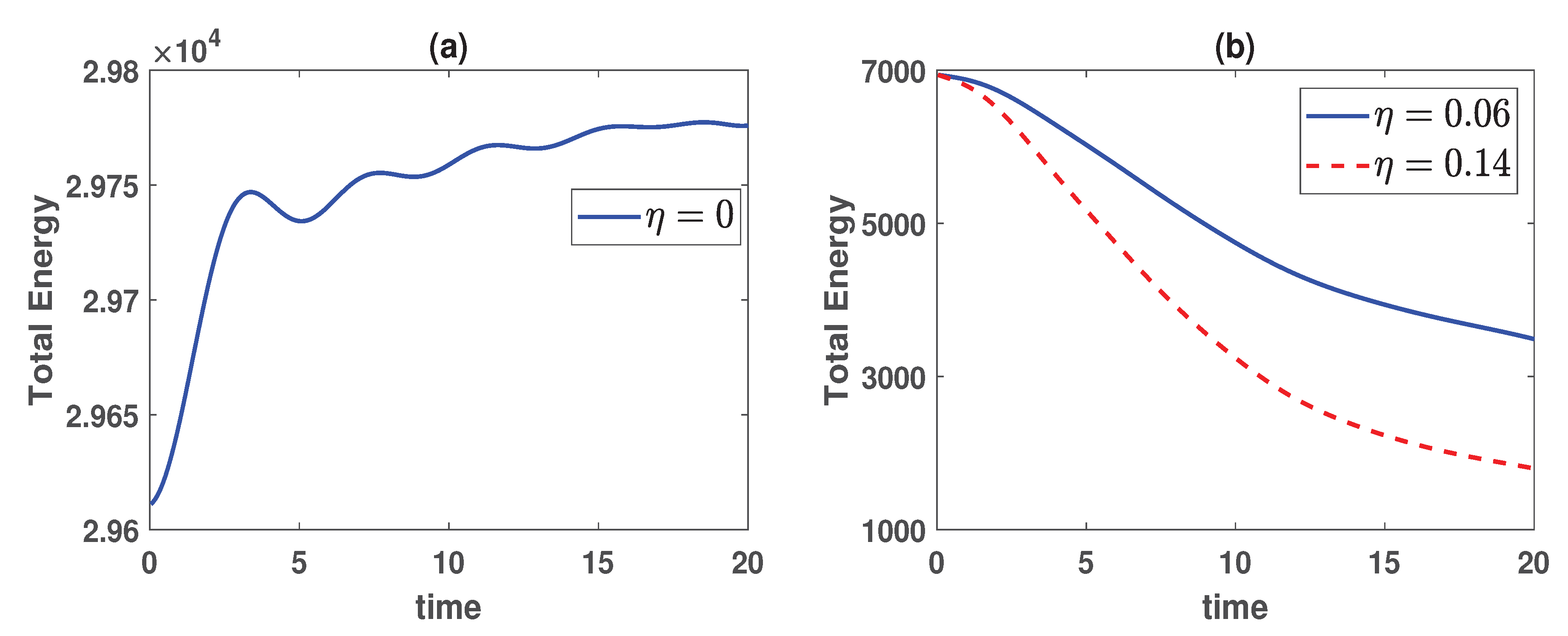
Figure 4.
Energy spectra of turbulence in the inertial range is shown. Subplot (a) shows the spectrum for , exhibiting a scaling, which is consistent with classical Kolmogorov turbulence. Subplot (b) shows the spectrum for , causing a steeper slope of , which signifies a turbulent decay.
Figure 4.
Energy spectra of turbulence in the inertial range is shown. Subplot (a) shows the spectrum for , exhibiting a scaling, which is consistent with classical Kolmogorov turbulence. Subplot (b) shows the spectrum for , causing a steeper slope of , which signifies a turbulent decay.
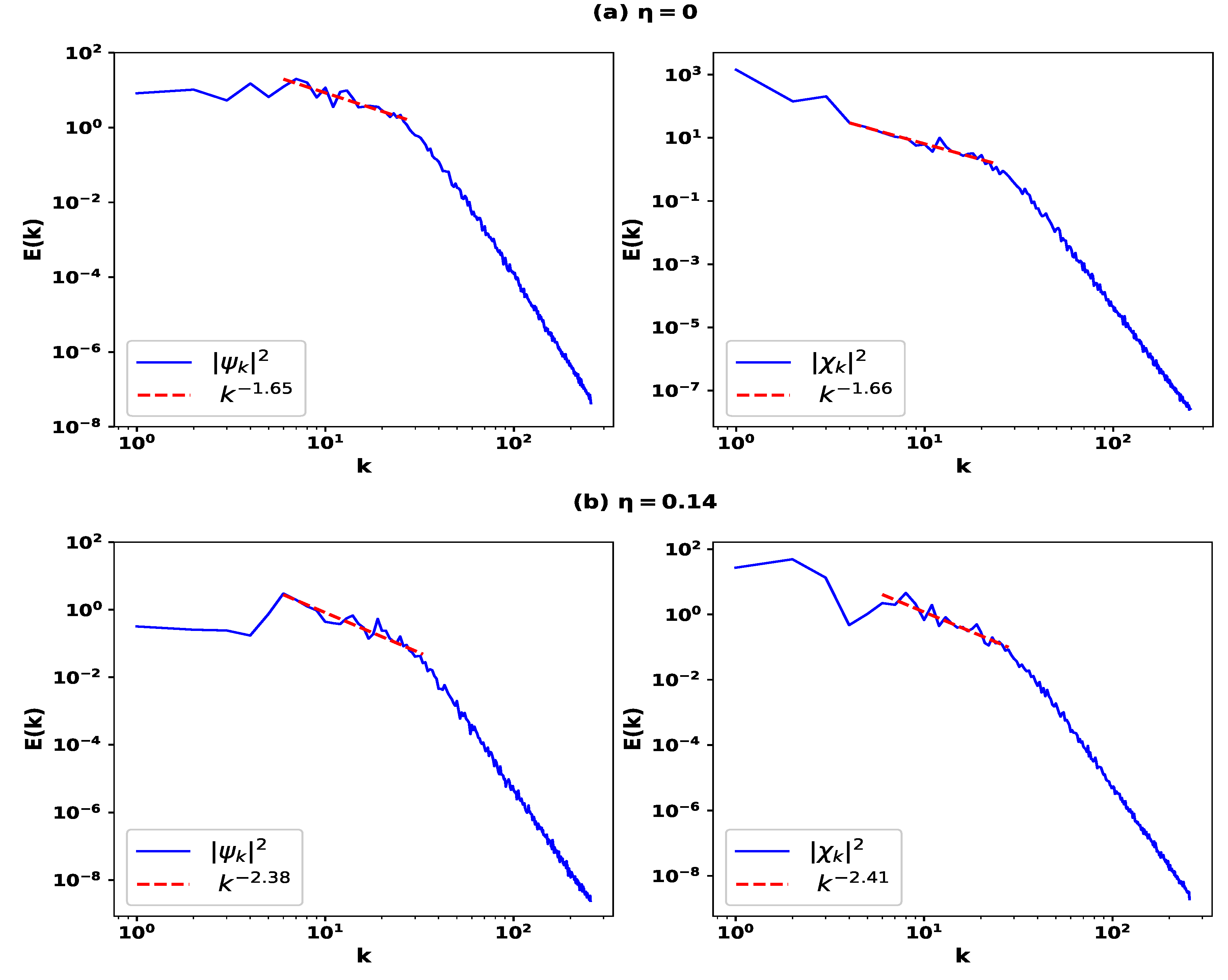
Figure 5.
The time evolution of the effective diffusion coefficient is shown for (left panel) and (right panel). Increasing the parameter , associated with Pedersen conductivity, results in reduced electron transport.
Figure 5.
The time evolution of the effective diffusion coefficient is shown for (left panel) and (right panel). Increasing the parameter , associated with Pedersen conductivity, results in reduced electron transport.
Disclaimer/Publisher’s Note: The statements, opinions and data contained in all publications are solely those of the individual author(s) and contributor(s) and not of MDPI and/or the editor(s). MDPI and/or the editor(s) disclaim responsibility for any injury to people or property resulting from any ideas, methods, instructions or products referred to in the content. |
© 2025 by the authors. Licensee MDPI, Basel, Switzerland. This article is an open access article distributed under the terms and conditions of the Creative Commons Attribution (CC BY) license (http://creativecommons.org/licenses/by/4.0/).
Copyright: This open access article is published under a Creative Commons CC BY 4.0 license, which permit the free download, distribution, and reuse, provided that the author and preprint are cited in any reuse.


