
Submitted:
15 October 2025
Posted:
17 October 2025
You are already at the latest version
Abstract
Equivalence test is a crucial concept in coding theorem, however its computation is bedeviled with bottlenecks such as its runtime complexity as a result of using combinatorial algorithms. To resolve this, the study proposes an equivalence testing framework for Linear code using Graph Neural Network (GNN). The proposed framework was assessed with focus on its effectiveness and generalization capabilities. Across the five runs, the framework yielded models which consistently achieved strong performance metrics, including an average accuracy of 99.576%, F1-score of 99.616%, and a ROC AUC score of 1.000. These results underscore the framework’s robustness and its ability to reliably detect equivalence between linear codes under coordinate permutation. The resulting model was then compared to two established linear code equivalence testing methodologies - namely Support Splitting Algorithm and Canonical Form approach, which further affirm the efficiency of the proposed GNN-based method.
Keywords:
linear codes
; code equivalency
; codewords
; Graph Neural Network
; Graph Isomorpishm Network
1. Introduction
Linear code equivalence (LCE) problem involves determining whether two linear error-correcting codes are the same under relabeling of coordinates or a scaling of coordinates for non binary fields (Bennett et al. 2024; Nowakowski 2024). LCE is crucial not only in coding theory but also in cryptography, this is due to its contribution in several code-based cryptosystems which rely on the hardness of code equivalence for security (Bennett et al. 2024). To solve LCE, the problem has been approached with combinatorial algorithms, methodologies like Sendrier’s support splitting Algorithm (SSA) solves code equivalence problem in polynomial time by exploiting structural invariants of the code (Nowakowski 2024). However, these methods struggle or become exponential on specially structured worstcase codes. It is crucial to note that Linear code equivalence problem (LCE) has been proven to be as hard as the Graph Isomorphism (GI) problem in a fine-grained sense, This implies that a general solution is unlikely to be easy.
Bennett et al. (2024) shows how mapping graphs to their incidence-matrix codes yields a reduction from Graph Isomorphism to Linear Code Equivalence. The authors further opined that the cycle code (kernel of graph incidence matrix) has minimal codewords exactly as the graph’s simple cycles, implying that the code encodes graphic matriod. In the same vein Kaski and Ostergard (2006) give a simple reduction similar to Bennett et al. (2024) indicating that if the input graphs are sufficiently connected, the transpose of the incidence matrices can be taken as generator matrices for binary codes.
Given this backdrop, there is a growing interest in leveraging machine learning techniques, especially Graph Neural Networks (GNNs) to tackle structural equivalence problem. GNNs are special type of neural models that operate on graph structure data and have proven effective in learning representations that capture graph topology and node features (Xu et al. 2018), Alluding to this is a study where Kipf and Welling (2017)’s Graph Convolutional Network applied convulational filters on graphs, yielding hidden representations that explicitly capture local graph structure and node attributes, also in a study by Xu et al. (2021) where the researchers studied automorphic equivalence (a formal notion of structural equivalence where nodes share identical structural roles) and show that standard GNNs fail to capture it hence the researchers proposed the GRAPE model, a GNN variant with special aggregators that explicitly differentiate neighbours having the same automorphic-equivalence pattern. Similarly, representation-learning methods have been developed to preserve structural identity: for example, A study by Ribeiro et al. (2017) that proposed a scheme called Struc2Vec which explicitly learns node embeddings so that structurally equivalent nodes have similar vectors, in this case Struc2Vec could identify structurally similar nodes across a graph—even if they are far apart.
Recent research publications in GNN expressiveness indicate that carefully designed GNNs can distinguish graph structures almost as powerfully as classic graph isomorphism tests, for instance, Xu et al. (2018) showed that standard GNNs (e.g. GCN, GraphSAGE) cannot distinguish certain non-isomorphic graphs, whereas their Graph Isomorphism Network (GIN) has been shown to be as powerful as the 1-WL test. Concretely, Xu et al. (2018) further proved that GIN – which aggregates neighbor features with injective MLPs – matches the WL power (1-WL) for graph isomorphism. In practice GIN achieves state-of-the-art graph classification accuracy while attaining this theoretical 1-WL limit Xu et al. (2018). This creates possibility of using GNNs to learn a notion of code isomorphism by representing codes as graphs and training the network to deduce when two graphs (codes) are equivalent.
This study focuses on designing a GNN based linear code equivalence testing framework and further outline how Bipartite Graph representation of binary linear codes can be transformed into a trainable format for Graph Neural Network.
1.1. Graph Neural Networks for Structural Learning
Graph Neural Network is a powerful tool for representations of graph structured data. When compared to other traditional neural networks which operate on fixed-size factor vectors or grids, GNNs perform message-passing over the nodes of a graph, aggregating information from neighbours to learn node embeddings and finally graph-level embeddings.
Basically, GNN typically follows a neighbourhood aggregation or message-passing scheme, where each node iteratively updates its feature vector by merging with features of its neighbours. After k layers, a node’s representation reflects information from its k-hop neighbourhood, and a graph-level embedding is obtained by pooling over all node features (Xu et al. 2018). The neighbourhood aggregation mechanism enables GNNs to effectively capture the structural features of a node’s local neighbourhood. As more layers are added, the receptive field of each node expands, enabling the network to progressively learn higher-order dependencies and global connectivity patterns accross the graph. A key concern in the theory of GNNs is how they distinguish different graph structures - essentially their expressive power in tasks similar to graph isomorphism testing. It has been proven that popular GNN variants such as Graph Convolutional Network (GCN) and GraphSAGE have limitations in identifying certain graph structures, this is as a result of mapping some non-isomorphic graphs to the same embedding due to the inherent constraints of message-passing scheme. To overcome this limitation Xu et al. (2018) introduced the Graph Isomorphism Network (GIN) which is a powerful GNN architecture designed to be as expressive as the 1-WL test. GIN uses sum aggregator for neighbourhood aggregation, rather than averaging or taking max. The sum function used in this research over a multiset of neighbor features is injective, so it ensure that no two different multisets will produce the same sum. By using sum aggregation combined with an injective readout function, k-layer GIN can theoretically distinguish any two graphs that the 1-WL method can distinguish after k iterations. Empirically, Xu et al. (2018) demonstrated that GIN indeed outperformed or matched other GNNs on graph classification benchmarks, validating that enhanced theoretical expressiveness can translate into strong practical performance. In addition to the sum aggregation, Xu et al. (2018) combined multi-layer perceptron (MLP) to mode universal multiset functions. This approach guarantees injectivity under mild conditions and therefore satisfies two key requirements i.e. Injective neighbourhood aggregation function and Injective readout function for graph-level representation. The core GIN update rule is given by
This formulation is the main distinct feature of GIN and other popular GNN variants such as Graph Convolutional Networks and GraphSAGE and it ensures that two structurally different neighbourhoods will be mapped to distinct embeddings, thereby capturing rooted subtree structures analogous to those in the WL test.
With these findings in mind, this research will ensure that the framework being developed gives blueprint for designing GNNs with archietecture that are at least as discriminate as WL. Futhermore Xu et al. (2018) study suggest that using GNN layers that are maximally expressive (such as the GIN or its variants) will enhance equivalence and non equivalence detection due to the fact that the network has a chance to produce different representations for linear code graphs.
Beyond 1-WL, researchers have explored extensions to make GNNs even more expressive. Morris et al. (2018) presented a theoretical study on the expressiveness of GNNs, establishing their relationship with Weisfeiler-Leman (WL) graph isomorphism. Morris et al. (2018) introduce a higher-dimensional GNN framework known as k-GNNs, based on the k-dimensional Weisfeiler-Leman test (k-WL). In contrast to 1-WL which updates node labels using neighbourhood aggregation, k-WL operates over k-tuples of nodes thereby enabling the model to capture higher-order graph structures such as motifs, subgraph symmetries, and community-level dependencies. The proposed archietecture by Morris et al. (2018) translates into neural form by allowing message passing across node tuples rather than single-node neighbourhoods. Each k-GNN iteration aggregates information across subgraphs of size k, thereby encoding relational patterns that are invisible to 1-WL and Classical GNNs. The researcher finally demonstrated that k-GNNs are strictly more expressive than GNNs and 1-WL, Morris et al. (2018) results extend prior knowledge of GNN expressiveness by introducing a general, theoretically grounded framework that encompasses both classical and higher-order archietectures.
Zopf (2022) in a comprehensive reviewed discussed higher order GNN with advanced archietecture that incoporate subgraph structures or attention mechanisms to go beyong 1-WL limitations. However (Zopf 2022) highlighted methodologies which include 2-WL and 3-WL which require manipulating and comparing pairs/triples, Motif-based representation, Subgraph sampling methods and Non-anonymous Node ID use, all come at a higher computational cost. Given this, our study focuses on using well-chossen message passing GNN archietecture. It is worth mentioning that in practice, manay real-world graphs are distinguishable by 1-WL or by minor enhancements like incorporating node degree or other simple invariants as features.
Summarily, we can affirm that GNN archietecture with maximal expressiveness is capable of evaluating equivalence and hence chosen for our framework.
1.2. Code Equivalence and Isomorphism Testing
Linear code equivalence (LCE) problem has a rich history in coding theory and has equally gained prominence in cryptography as well. LCE problem can be in two folds namely: Permutation Code Equivalence (PCE) which enable permutation of code coordinates, and Linear/Monomial Code Equivalence (LCE) which uses permutation together with multiplication of coordinates by non zero scalars (monomial transformation) (Bennett et al. 2024). For binary codes which applies to this study, these two notions coincide because multiplying a coordinate by the only non zero scalar (1) has no effect on the code. This concept is not known to be NP-complete; rather it is NP and possesses a similar status as the Graph Isomorphism problem. Alluding to this submission is a reduction from Graph Isomorphism to Linear Code Equivalence as shown by (Bennett et al. 2024).
Algorithmic approaches to code equivalence do exploit invariants of codes, one of those approaches is (Sendrier 2000; Barenghi et al. 2020), who introduced the Support Splittig Algorithm (SSA). SSA operates by iteratively partitioning the coordinate positions of the code based on the code’s structural properties such as the support of codewords as well as the coordinates they involve. When two codes are equivalent, they should have the same set of invariant parameters such as weight distribution and higher order invariant. SSA can match up coordinates by looking at the patterns of which positions appear together in codewords, also it has been proven that SSA solves random instances of permutation equivalence efficiently with high probability, this implies that for a generic pair of random codes, the algorithm is likely to find the equivalence (or conclude non-equivalence). However with the effectiveness of SSA, there are specially constructed codes which are often with high symmetry where SSA can stall and require exponential time (Nowakowski 2024).
SSA core idea is to exploit structural invariant of codes to iteratively split the support into smaller subsets that must correspond under any valid permutation. By refining coordinate partitions using such invariants, SSA narrows down the possible mappings. Eventually, it assigns coordinates of to coordinates of in a consistent way, finding the permutation if one exists.
Algorithmically, SSA proceeds recursively: it selects a coordinate (or a set of coordinates) as a “distinguishing” set, splits the remaining coordinates into classes based on an invariant (like the presence or absence in supports of low-weight codewords, or membership in the hull), and then recurses on each class (Chou et al. 2023). Considering the mode of operation of SSA as outlined below in Algorithm 1, it is described support splitting because it recursively partitions code’s support.
| Algorithm 1: Support Splitting Algorithm (SSA) |
|
In practice, SSA is very efficient for generic random codes. It runs in polynomial time with high probability on random instances of Permutation Code Equivalence (PCE) (Nowakowski 2024), especially when the codes have a small hull (Cheraghchi et al. 2025). However, SSA’s performance degrades on highly symmetric codes. If the code’s hull is large (particularly in the extreme case of a self-dual code where the hull equals the whole code), the usual invariants do not differentiate coordinates, and the algorithm essentially has to brute-force the permutation. In such worst cases SSA requires exponential time, on the order of operations (roughly ) for a code (Chou et al. 2023).
Other than SSA, other methodologies include canonical form approaches, where each code is converted into some canonical representative form and then compared. Recent research by Chou et al. (2023) has considered improved algorithms using such canonical forms as well as information set decoding techniques to handle code equivalence more efficiently for some parameter ranges. For instance, the algorithm by Chou et al. (2023) was efficient for large field sizes q, and Nowakowski (2024) improved it for smaller fields including binary linear code thereby achieving optimal runtime. These reported advancements are largely theoretical and complex to implement, howevery they provide insight that code equivalence, while hard in general posseses exploitable structure.
In the context of framework being developed, these algorithmic methodologies for the baseline; i.e they guarantee to deduce equivalence if one exists, but is infeasible for large code lengths due to combinatorial explosion. A learned approach with GNNs could learn to imitate these heuristics or find its own heuristics thereby pottentially solving typical cases much faster. For example, a GNN might implicitly learn to detect patterns similar to those SSA looks for (like groups of coordinates that share many common codewords) by virtue of how it aggregats information in the graphical representation.
Another aspect worth noting from literature is that code equivalence can also be related to matroid isomorphism, since linear codes correspond to binary matroids. This correspond to Bennett et al. (2024) research where the researchers mention reduction between code equivalence and linear lattice isomorphism, this further hint at deep combinatorial structure underlying graphs, codes, lattices and matroids. From this findings, the idea of representing codes as graph is a natural thing to do - it is essentially converting one isomorphism problem (codes) into another (graph), where graph based technique can be applied.
Summarily, the literature on code equivalence provides the problem’s complexity context and algorithmic approaches that exist. Reviwed litreature show strong support for this study, indicating that while an exact efficient algorithm is unknown, many practical instances can be solved with heuristic or partically exponential methods. The framework being developed in this study will be another promising approach - heuristic in nature but pottentially powerful.
1.3. Data Representation Pipelines of GNNs
To implement a GNN solution, careful preparation of data is required. Graphical structures are not as straightfoward to feed into neural network as image or text; it is required that the graph’s structures must be encoded into tensor form. It is crucial to note that modern libraries have been developed to streamline this process. Medium (2022) revealed that pyTorch Geometric(PyG) is built on pytorch and provides a high-level interface for handling graphs. In PyG, a graph is typically represented by an object that contains at least two components: X which is a matrix of node features with its dimension being number of node by feature dimension and edge_index, a matrix that lists graph edges indicating source and target node indices. PyG makes available convenient data loaders that can batch multiple graphs together for training. It does so by creating a big disjoint graph (stacking the edge indices and adjusting indices for each graph) and maintaining a batch vector that indicates which graph each node belongs to (Exxact 2023). This way, standard mini-batch gradient descent can be applied even though each training example might be a graph of different size. PyG is known for its ease of use, as it integrates well with PyTorch’s ecosystem. It offers a variety of pre-built GNN layers (GCNConv, GraphSAGE, GAT, GINConv, etc.) and utilities for common tasks like train/test split, transformations, etc. In fact, PyG’s philosophy is to make working with graphs feel as natural as working with tensors in PyTorch (Exxact 2023). The library covers a wide range of applications and is actively maintained, making it a strong candidate for our framework. Using PyG, we can create a custom Dataset that reads graphical data (possibly from files or generated during runtime) and returns Data objects for each graph (Medium 2022). The Data object in this case would contain:
- x: Node features matrix. Each node in the graph is indicated here with a feature indicating its type (bit or check). This could be a one-hot vector of length 2, or even just a single binary value that is 0 for bit-nodes and 1 for check-nodes .
- edge_index: Edge list. The edge index will be a 2×E tensor where each column is (source_node, target_node). In an undirected Tanner graph, Each edge are created twice in this list (one from bit to check, one vice versa) or use a convention that edges are undirected in the convolution (some libraries treat edge_index as undirected if you add both directions).
PyG also allows us to easily implement a pair of graphs scenario. We have a couple of options: we can either create a single graph that is the disjoint union of the two graphical representations and somehow mark or connect them, or we can process them separately and then combine embeddings. A straightforward approach is a Siamese network style: the dataset could yield pairs of Data objects along with a label (equivalent or not). One can write a custom training loop where for each pair, we feed each graph through the GNN (which will share weights) and then compare the outputs. To leverage PyG’s batching, another approach is to construct a single Data that contains the union of two graphs plus an indicator of which graph each node belongs to, then design the GNN or subsequent layers to produce two outputs. However, conceptually, treating it as two separate graphs may be cleaner.
Deep Graph Library (DGL) is another framework that is more agnostic, in the sense it can work with PyTorch, TensorFlow, or MXNet as a backend. DGL provides a graph object where one can store node and edge features, and it handles batching by a similar mechanism of disjoint union graphs. DGL emphasizes performance – its design focuses on efficient sparse operations and it often achieves very high speed on graph tasks (Wang et al. 2019). DGL uses the concept of message functions and reduce functions which the user can specify, or one can use its own layers. It also has a notion of heterograph – supporting multiple node types and edge types in a single graph. This could be directly applicable to Tanner graphs, which naturally have two node types. Instead of treating it as a homogeneous graph with a feature flag, we could define a DGL heterograph with one node type for bits and one for checks, and one edge type for the incidence. The advantage is that we could then have different learnable transformations for messages passing from bit to check versus check to bit if we wanted to. PyG can also handle heterographs (to a lesser extent, via its HeteroData structures), but DGL is built around that concept. Both PyG and DGL would allow us to implement the needed pipeline.
It is also worth noting that when converting data for GNNs, one must ensure not to inadvertently inject any information that breaks the intended invariance. For instance, the node ordering or numbering in the graph data structure should not matter – a GNN’s output should be invariant to how nodes are indexed, as long as the graph structure is the same. In practice, GNN libraries maintain this invariance because they use only relative structure (neighbors, etc.), but if we were to supply node indices as features themselves, that would leak a particular labeling. We will avoid any such features; only structural features will be given.
To illustrate the pipeline concept, consider the steps enumerated by Apichonkit (2022) in a tutorial for PyG (Medium 2022):
- Read the graph data (in our case, perhaps from a JSON or from an in-memory object).
- Create the edge_index (understanding how PyG deals with graph connectivity is key).
- Create and process node attributes (categorical attributes like our node type can be one-hot encoded, numerical ones can be normalized).
- Add any additional information needed (like graph ID or target label).
- Finally, create a PyG Data object with the fields (x, edge_index, y, etc.) and, if using a custom dataset class, save it for reuse.
Understanding how x (node feature matrix) and edge_index work is crucial (Medium 2022), as these form the core of the graph representation in PyG. The index of a node in the edge_index array corresponds to the row in x for that node, so they must align. We will ensure that bit nodes occupy, say, indices 0 to in x and check nodes n to , so that it’s easy to interpret.
For open-source tools, as mentioned, PyG and DGL are primary candidates. We will likely choose PyG for illustration due to its simplicity and our familiarity. PyG’s documentation itself states that it is a library built to easily write and train GNNs for structured data pytorch-geometric.readthedocs.io. On the other hand, DGL’s design principles highlight performance and the graph-centric abstraction for optimization (Wang et al. 2019). Either would be suitable; choosing one may depend on practical considerations like compatibility with other code or personal preference.
In summary, the literature and practical guides on GNN data pipelines tells us how to go from Graphical representation GNN input. It emphasizes careful construction of edge indices and feature matrices (Medium 2022), the availability of batching and data handling in libraries, and the need to maintain invariances. These lessons will be applied in our methodology when we describe the implementation steps for the framework.
2. Methodology
In this section, methodologies adopted to design the equivalence testing framework using GNNs are discussed.
2.1. Input Graph Specification
Binary linear code can be represented using Bipartite graph, this graph structure contains all necessary information for equivalence testing and hence used as input for the framework. Below are the features of the required input graph:
- Nodes: The bipartite graphical representation of a code C contains two types of nodes represents position nodes one for each bit spaning from 1 to length (n). represents codeword node, one for each codeword in the linear code.
- Edges: An edge connects position node to codeword node if and only if the bit i has entry 1. In other words if then an edge is created between and .
2.2. GNN-Compatible Data Pipeline
With the bipartite graph defined, we now describe how to convert these graphs into a format suitable for input into a graph neural network, and outline the pipeline that takes raw graph data through model training and inference. As recommended by Medium (2022) due to its popularity and ease of use we will use PyTorch Geometric (PyG). The data pipeline consists of the following steps:
-
Data Preparation (Graph Construction): For each code’s bipartite graphical representation, objects with the following necessary information would be constructed:
- –
- Node indexing: Index the nodes such that position nodes have indices where n is the length of each codeword, and codeword nodes have indices . This gives a total of nodes per graph.
- –
- Edge index: Create a list of edge as pairs (source_node, target_node) following the bipartite graph’s edges. For each edge connecting codeword to bit position j such that , we add an entry . To ensure the graph is effectively undirected, we include both directions of each edge. I.e for every edge , we add both and to the edge list.
- –
- Node features: A feature is added to each node to indicate its type. The two-dimensional one-hot vector scheme is convenient and hence used: for a position node should be represented [1,0], and for a codeword node . This way, the GNN can easily distinguish position node and codeword node.
-
Representing Graph Pairs: Since the task involves determining if two codes (graphs) are equivalent, our model ultimately needs to look at pairs of Tanner graphs. There are two general strategies to feed pairs into the model:
- –
- Siamese Pair Handling: In this approach, we use two separate Data objects (one for each graph). Each graph is passed through the same GNN encoder to produce two embeddings. These embeddings are then compared—either outside the GNN or via a custom comparison layer. During training, we sample or load pairs of graphs along with a binary label: 1 if the graphs are equivalent, and 0 otherwise. Instead of using a single PyG DataLoader for graph pairs, we may use a wrapper to iterate through the pairs or create an index that yields graph pairs. The model effectively processes one graph at a time using shared weights (as in Siamese networks), followed by a learned or heuristic comparison between their embeddings.
- –
- Combined Graph Object: Alternatively, we can construct a single Data object that includes both graphs as disconnected components. For instance, suppose graph A has nodes and graph B has nodes. We then renumber graph B’s nodes to follow after A’s, and create a combined edge_index that includes edges for both graphs (but no cross-graph edges). The resulting graph has total nodes. A graph-level label indicates equivalence or non-equivalence. Optionally, a node-level feature can be added to distinguish which component (graph A or graph B) a node belongs to. However, because the components are disconnected, a GNN can theoretically infer this separation during message passing. When using PyG with batching, the internal batch vector still helps identify graph membership for each node.
Both strategies of representing graph pairs as discussed enable the model to process two graphs and output a decision. The Siamese approach is conceptually clean and easier to implement: each graph goes through an identical encoder, and the outputs are compared to determine equivalence. The combined-graph approach is also valid and can be useful in fully graph-based pipelines. However, we adopt the Siamese architecture for clarity (Medium 2022).
2.3. Proposed GNN-based Framework for Code Equivalence Detection
The proposed framework core is the Graph neural network that processes bipartite graph representations and determines if two graphs correspond to equivalent codes. In this section the archietecture is outlined including the GNN model for individual graphs and the mechanism for comparing the two graph representations.
Graph Neural Network Backbone: Graph Isomorphism Network (GIN) is used as the backbone for processing each bipartite graph representation. GINs are among the most expressive GNN variants for graph structure, essentially matching the discrimination power of the 1-dimensional Weisfeiler-Lehman test (Xu et al. 2018). GIN update rule is expressed as
where is the feature vector of node v at layer t, is the set of neighbor nodes of v, and each GIN layer uses a learnable Multi-layer Perceptron as its update function. Specifically, at each layer t, the node representation is updated by applying an MLP to the sum of the node’s own previous representation and those of its neighbors. Thus the MLP is part of the layer operation, serving as a non-linear transformation after aggregation (Xu et al. 2018). Intuitively, each GIN layer takes a node’s current representation and the sum of its neighbors’ representations, then passes this through an MLP to produce the next representation. The use of summation is key to GIN’s power – it can distinguish different neighbourhood structures better than, say, an averaging aggregator, because summing treats neighbor feature multisets in a way that preserves their uniqueness (Xu et al. 2018). Following Xu et al. (2018), we adopt a depth GIN layers in our model. Their work showed that using 3 to 5 layers allows the network to capture sufficient neighbourhood information without over-smooting - a phenonmenon where node representations become indistinguishable in deeper layers . Each node’s receptive field grows with each layer (1-hop per layer), so L layers means a node’s representation includes information from L-hop neighbors.
Bipartite Graph Consideration: The graphical representations used for this study are bipartite, with distinct position and codeword nodes. With this backdrop a specialized GNN that respect bipartite structure explicitly is required - for instance, alternate updates where position nodes only recieve messages from codeword node and vice versa. For this study a standard GIN that treats the graph as a homegenous graph, and rely on the node type feature (one-hot indicator) to let the network learn to differentiate message sources. In theory, the MLP in the GIN can learn to apply different weights based on the node’s type or its neighbors’ types (since those are part of the feature vector) (Xu et al. 2018).
Figure 1.
Proposed GNN-based Framework for Code Equivalence Detection.
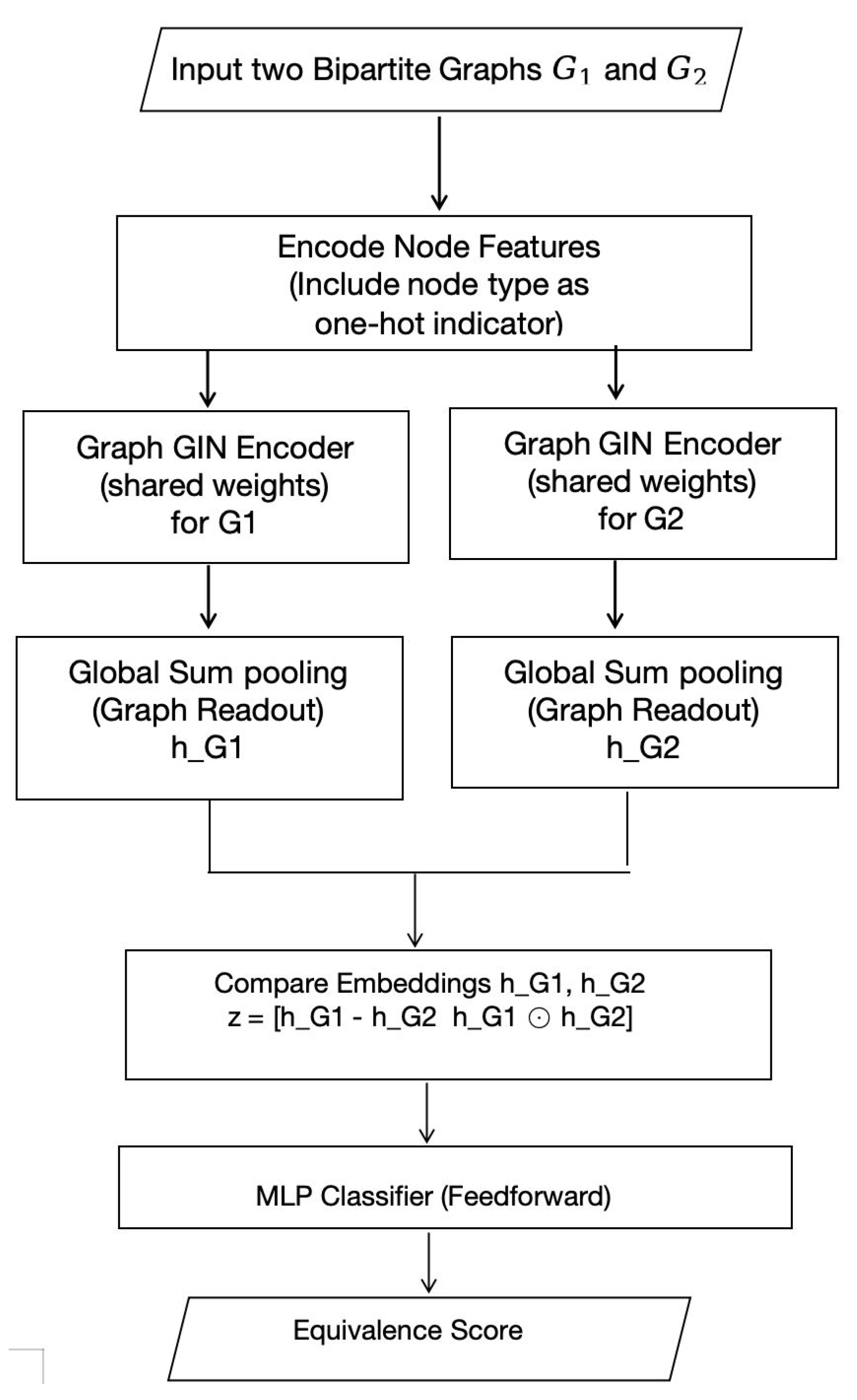
Global Pooling (Graph Readout): After L GIN layers, each node v in the graphical representation has a final embedding that reflects its local topology and features. These nodes are aggregate these node embeddings into a single vector representing the whole graph (the code). We use a global sum pooling operation:
This sums the embeddings of all nodes in the graph to produce a graph-level embedding . We choose sum pooling (as opposed to mean or max) to remain consistent with the GIN philosophy of using sum as an injective aggregator (Xu et al. 2018).
Comparing Two Graph Embeddings: To determine if two graphs and are equivalent, we compare their graph embeddings and . In a Siamese network architecture, we have two identical GNN streams (with shared weights) producing these embeddings. We then need a comparison function that outputs a similarity score or classification. A simple and effective design is to use the absolute difference and possibly the element-wise product of the embeddings as features, as mentioned above. Concretely, we form a vector:
where ∥ denotes concatenation and ⊙ denotes element-wise multiplication. This z vector now encapsulates how similar or different the two graph representations are in each dimension. We feed z into a small feedforward neural network (an MLP) to produce a single output logit.
In summary, the architecture workflow can be described as Pseudocode in Algorithm 2
| Algorithm 2: Pseudocode for GNN-Based Code Equivalence Detection |
|
2.4. Linear Code Dataset Description and Theoretical Validation
To ensure a robust and generalizable evaluation of the proposed framework, five independent datasets were generated. Each dataset is made up of labeled pairs of binary linear codes, with a labels indicating whether the two are equivalent(1) or non-equivalent (0). To assess consistency and reliability of the model under different randomized code constructions, The generated datasets were used in five seperate training and evaluation sessions. Each dataset contained between 4,000 and 5,000 test samples, along with a proportionally larger training set. In all five sessions, over 200,000 samples were used for model training and evaluation. The labels within each dataset were relatively balanced, with approximately 50-55% of the samples representing equivalent code pairs and 45-50% representing non-equivalent pairs. This balanced composition ensures effective supervised learning without introducing class bias.
Each linear code was represented as a set of codewords over the binary field , with each codeword formatted as a space-separated binary string. For equivalent code pairs (label=1), code B was generated by applying random permutation of bit positions to code A while for non-equivalent pairs (label=0), code B was generated independently to ensure structural dissimilarity from code A.
To affirm the mathematical and coding-theoretic integrity of these codes, each was synthetically generated and subjected to validation using Gilbert-Varshamov bound. Specifically the codes were constructed such that they possess parameters where:
- n is the codeword length
- k is the dimension
- d is the minimum Hamming distance between any two distinct codewords
Each code was validated to meet the Gilbert–Varshamov existence condition:
2.5. Relationship between Linear Code Equivalence and Graph Isomorphism
We now formally establish that the problem of testing linear code equivalence under coordinate permutation can be reduced to the problem of testing isomorphism between their bipartite graphical representations.
Theorem. Let be two binary linear codes. Let denote their bipartite graph representations. Then:
where means that the graphs are isomorphic under a permutation acting only on the position (bit) nodes.
Proof. Suppose . By definition of code equivalence, there exists a permutation such that:
Now consider the bipartite graph , where:
- : position nodes
- : codeword nodes (one for each codeword)
- if and only if codeword has
Define a new graph by permuting the position nodes of using . Specifically, for every edge , map it to . The resulting graph has the same structure as , since the bit positions in each codeword of have been permuted in exactly the way needed to match the bit positions of corresponding codewords in . Hence:
Thus, .
Conversely, suppose , meaning there exists a bijection such that adjacency is preserved between position nodes and codeword nodes. Then, for each codeword in , the set of connected bit positions corresponds exactly (under ) to the positions connected to the corresponding codeword node in . This implies that each codeword in is a bit-permuted version of some codeword in , and vice versa. Therefore:
Hence, .
This theorem confirms that binary linear code equivalence under position permutation is exactly characterized by graph isomorphism of their bipartite representations. Thus, graph-based models, such as GNNs, can be leveraged to learn code equivalence via graph isomorphism detection.
2.6. Theoretical Proof: Learnability of Bipatite Graph Matrix Representation by a GNN
Let be a binary linear code of dimension k, represented by a set of codewords . Define the corresponding graph as a bipartite graph with:
-
, where:
- –
- is the set of position (bit) nodes
- –
- is the set of codeword nodes (one for each codeword used)
- , with edge if and only if bit i is 1 in codeword .
2.6.1. Bipartite Graph Matrix Formulation
Define the adjacency matrix of the graph as:
where is the binary incidence matrix such that iff bit participates in codeword .
Define the node feature matrix such that:
2.6.2. GNN Processing on Matrix Representation
Let be a Graph Neural Network (e.g., a GIN) operating on the matrix pair. GNN layers update node embeddings as:
where:
- is the normalized adjacency matrix (e.g., via degree normalization),
- is a learnable weight matrix,
- is a nonlinear activation (e.g., ReLU).
By stacking such layers and applying pooling ( sum ), we obtain a graph-level embedding .
2.6.3. Permutation Invariance
Let be a permutation matrix. A relabeling of nodes corresponds to:
For any isomorphic graphs , the GNN satisfies:
Equation (12) ensures that code equivalence under bit permutation is preserved in the learned representation.
2.6.4. Expressiveness for Equivalence Testing
From the results of Xu et al. (2019), the Graph Isomorphism Network (GIN) is provably as powerful as the 1-Weisfeiler-Lehman (1-WL) test. Thus, if two Bipartite graphs are not isomorphic, a sufficiently deep GIN will learn .
Theorem. Let be the matrix representation of the Bipartite graph of a binary linear code. Then, there exists a GNN f such that for any codes :
- If (i.e., equivalent), then
- If , then
provided that and are constructed as above and f is an injective GNN architecture (e.g., GIN).
The Bipartite matrix representation is GNN-learnable, encoding all structural information necessary for equivalence testing while preserving permutation invariance.
2.6.5. Dataset Fields
Each row in the dataset contains:
- code_A: A space-separated list of binary strings representing valid codewords of a linear code A.
- code_B: A corresponding list of codewords for code B.
- label: A binary value, where 1 indicates that codes A and B are equivalent (i.e., one can be transformed into the other via a permutation of bit positions), and 0 indicates they are non-equivalent.
2.7. Computational Environment
All experiments, including dataset generation, training, and evaluation, were conducted using Google Colab Pro with GPU acceleration enabled. The computational environment is summarized below:
- System RAM: 12.7 GB
- GPU RAM: 15.0 GB (NVIDIA Tesla T4 or A100, depending on session allocation)
- Disk Space Available: 112.6 GB
-
Software Stack:
- –
- Python 3.10
- –
- PyTorch 2.x
- –
- PyTorch Geometric 2.x
- –
- CUDA Toolkit (when GPU runtime enabled)
The use of GPU acceleration significantly reduced training and inference time, particularly for deeper Graph Neural Network (GNN) architectures and larger bipartite graph representations. All model training and runtime benchmarking scripts were executed in this controlled environment to ensure consistency and reproducibility.
3. Results and Discussion
3.1. Training and Validation Performance
Figure 2 illustrates the dynamics across all five training session, both training and validation loss consistently decreased and then stabilized with minimal signs of overfitting. The validation F1-scores reached and maintained high values within the first 20 epochs, while the validation AUC approached 1.0, indicating strong classification confidence.
3.2. Aggregate Test Performance
Following the traning, each model was evaluated on its respective test set. The average accuracy, precision,recall, F1-Score and ROC AUC score are , , , and respectively. These results demonstrate consistenly strong discriminative capacity across multiple randomized linear code datasets. It is crucial to note that recall being near-perfect indicates that the model correctly identified almost all equivalent code pairs. This is important for systems that require strict minimization of false negatives.
3.3. ROC Curve Analysis
Figure 3 shows the Receiver Operating Characteristic (ROC) curve from one of the evaluation runs. All the training sessions conducted produced ROC AUC scores close to 1.0, confirming near-perfect separability of equivalent and non-equivalent codes.
3.4. Confusion Matrix and Test Metrics
The average classification performance across the five sessions indicates high precision and recall for both "Equivalent" and "Not Equivalent" classes Table 1 summarizes these per-class metrics.
These metrics suggest minimal misclassification, with excellent balance between sensitivity and specificity. The model’s capacity to generalize across distinct tests sets underscores its practical applicability to diverse code datasets.
3.5. Runtime Analysis
Table 2 shows the runtime (in seconds) taken by each method to determine equivalence between two linear codes for various values of n. All input code pairs were designed to be equivalent under coordinate permutations.
Figure 4 compares the runtime of three linear code equivalence testing methods—Support Splitting Algorithm (SSA) Sendrier (2000), Canonical Equivalence Chou et al. (2023), and the proposed GNN-based model across varying code lengths. The vertical axis is presented on a logarithmic scale to capture the large disparities in performance across methods.
3.5.1. Observations
- SSA Performance: The SSA method exhibits exponential growth in runtime, with evaluation time increasing rapidly as n grows. For , SSA required approximately 14.3 seconds, and beyond , the method becomes computationally infeasible within a reasonable time frame. This runtime behaviour can be attributted to combinatorial explosion i.e. examining invariants derived from supports of codewords and attempting to refine partitions based on these support hence as n increases, the number of codewords and support combinations grows exponentially, also the exponential spike in runtime can be further attributed to the recursive split operation of SSA which recursively splits support sets and matches them accross codes. This recursive branching creates a backtracking-style search tree, which scales poorly.
- Canonical Performance: The Canonical Form approach demonstrates exponential runtime growth similar to SSA. For example, at , the runtime exceeds 1000 seconds. This reveals a scalability bottleneck, especially under coordinate permutation equivalence, where canonical labeling becomes computationally intensive. Canonical form approach requires transforming codes into graphs and find a unique canonical label under coordinate permutations, and with the space of coordinate permutation being , the approach will struggle with dense code representations, also the approach operates globally on code structure hence does not scale well with input size.
- GNN Model: The proposed GNN-based approach maintains stable and efficient runtimes across all tested code lengths. Even at higher dimensions, the runtime remains under 0.07 seconds, benefiting from parallel execution and model generalization. This suggests its suitability for real-time or large-scale equivalence testing. Due to this approach’s mode of operation: the model learns to recognize equivalence patterns without exhaustive enumeration, exploiting features of the graph structure, also due to its generalization ability, the model applies a constant-time forward pass for inference, independent of the underlying combinatorial complexity.
4. Conclusion
This study sought to design an equivalence testing framework for Linear code using Graph Neural Network (GNN). To achieve this and establish the required theoretical background, related literature was reviewed and this further affirms the relevance of this research. The Architecture of the proposed framework was extensively outlined with GNN variant Graph Isomorphism Network being the core component of the framework. The framework was subsequently implemented using Python libraries.
To assess the effectiveness and generalization capability of the proposed framework, five independently generated datasets were used for training and evaluation. Each dataset consisted of thousands of labeled linear code pairs, constructed and validated using the Gilbert–Varshamov bound to ensure theoretical correctness. Across the five runs, the model consistently achieved strong performance metrics, including an average accuracy of 99.576%, F1-score of 99.616%, and a ROC AUC score of 1.000. These results underscore the framework’s robustness and its ability to reliably detect equivalence between linear codes under coordinate permutation. The resulting model was then compared to two established linear code equivalence testing methodologies - namely Support Splitting Algorithm and Canonical Form approach, which further affirm the efficiency of the proposed GNN-based method.
References
- Bennett, H.; Myat, K.; Win, H. Relating Code Equivalence to Other Isomorphism Problems 2024.
- Nowakowski, J. An Improved Algorithm for Code Equivalence. Cryptology ePrint Archive 2024.
- Kaski, P.; Ostergard, P.R.J. Classification Algorithms for Codes and Designs; Springer-Verlag, 2006. [CrossRef]
- Xu, K.; Jegelka, S.; Hu, W.; Leskovec, J. How Powerful are Graph Neural Networks? 7th International Conference on Learning Representations, ICLR 2019 2018.
- Kipf, T.N.; Welling, M. Semi-Supervised Classification with Graph Convolutional Networks, 2017.
- Xu, F.; Yao, Q.; Hui, P.; Li, Y. Automorphic Equivalence-aware Graph Neural Network 2021.
- Ribeiro, L.F.R.; Savarese, P.H.P.; Figueiredo, D.R. struc2vec: Learning Node Representations from Structural Identity. Proceedings of the ACM SIGKDD International Conference on Knowledge Discovery and Data Mining 2017, Part F129685, 385–394. [CrossRef]
- Morris, C.; Ritzert, M.; Fey, M.; Hamilton, W.L.; Lenssen, J.E.; Rattan, G.; Grohe, M. Weisfeiler and Leman Go Neural: Higher-order Graph Neural Networks. 33rd AAAI Conference on Artificial Intelligence, AAAI 2019, 31st Innovative Applications of Artificial Intelligence Conference, IAAI 2019 and the 9th AAAI Symposium on Educational Advances in Artificial Intelligence, EAAI 2019 2018, pp. 4602–4609. [CrossRef]
- Zopf, M. 1-WL Expressiveness Is (Almost) All You Need. Proceedings of the International Joint Conference on Neural Networks 2022, 2022-July. [CrossRef]
- Sendrier, N. Finding the permutation between equivalent linear codes: the support splitting algorithm. IEEE Transactions on Information Theory 2000, pp. 1193–1203. [CrossRef]
- Barenghi, A.; Biasse, J.F.; Persichetti, E.; Santini, P. ON THE COMPUTATIONAL HARDNESS OF THE CODE EQUIVALENCE PROBLEM IN CRYPTOGRAPHY. Advances in Mathematics of Communications 2020.
- Chou, T.; Persichetti, E.; Santini, P. On Linear Equivalence, Canonical Forms, and Digital Signatures. Cryptology ePrint Archive 2023.
- Cheraghchi, M.; Shagrithaya, N.; Veliche, A. Reductions Between Code Equivalence Problems 2025.
- Medium. First-timer’s Guide to Pytorch-geometric — Part 1 The Basic | by Mill Apichonkit | CJ Express Tech (TILDI) | Medium, 2022.
- Exxact. PyTorch Geometric vs Deep Graph Library | Exxact Blog, 2023.
- Wang, M.; Zheng, D.; Ye, Z.; Gan, Q.; Li, M.; Song, X.; Zhou, J.; Ma, C.; Yu, L.; Gai, Y.; et al. Deep Graph Library: A Graph-Centric, Highly-Performant Package for Graph Neural Networks 2019.
Figure 2.
Training and validation loss, F1-score, and validation AUC 5 training sessions
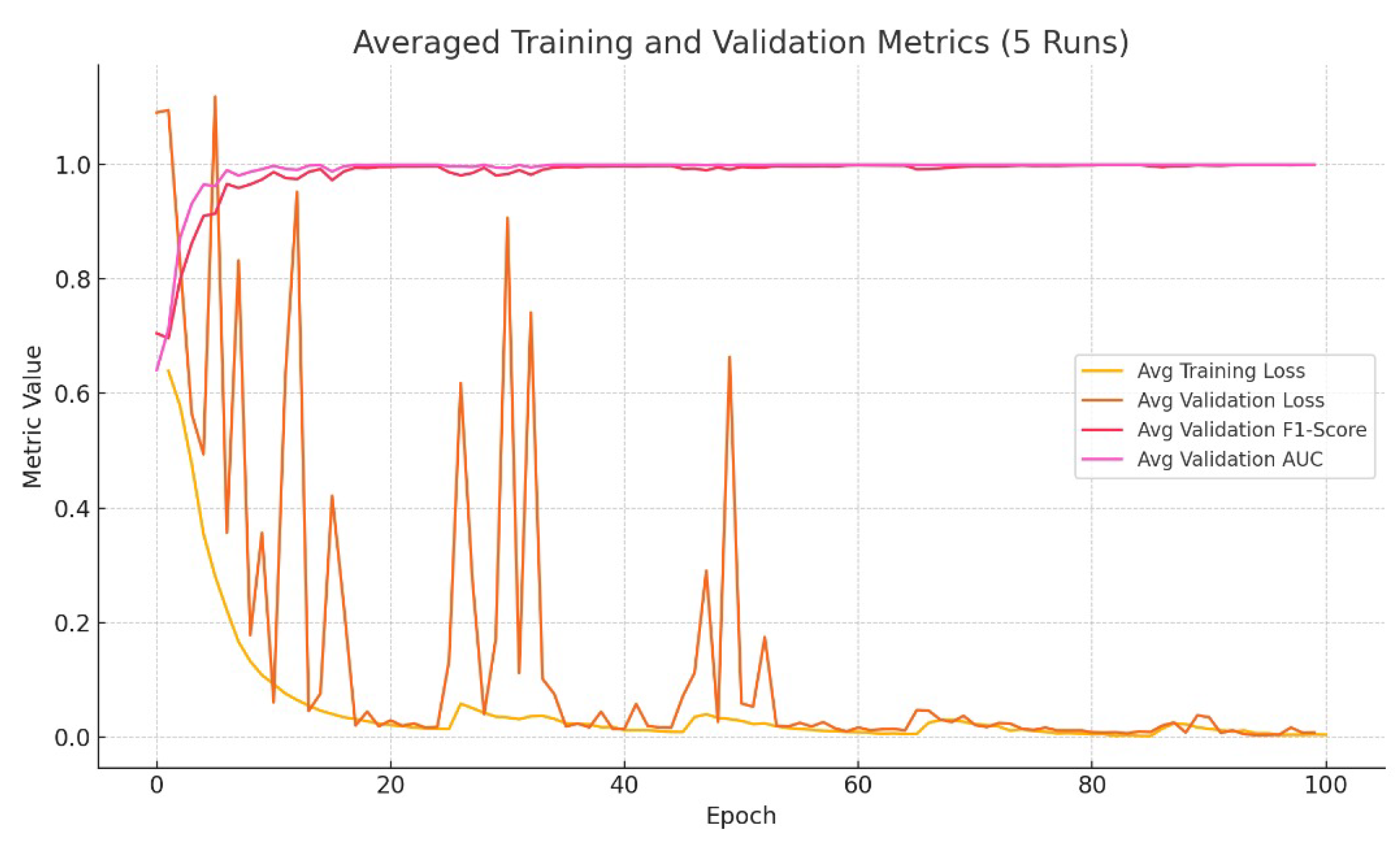
Figure 3.
ROC curve showing high model discriminability (AUC = 0.999).
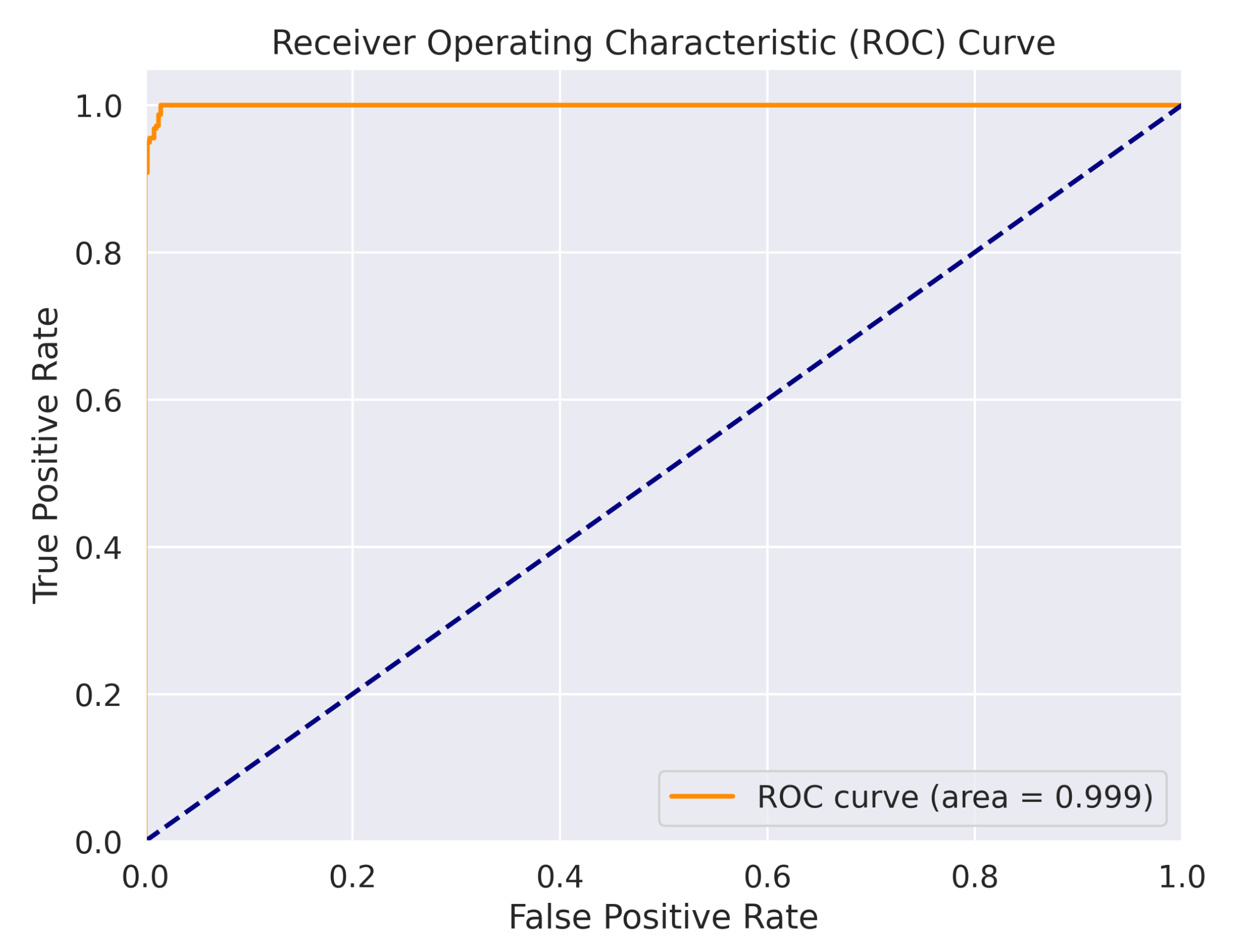
Figure 4.
Log-scale runtime comparison of SSA, Canonical, and GNN methods across code lengths to 14.
Figure 4.
Log-scale runtime comparison of SSA, Canonical, and GNN methods across code lengths to 14.
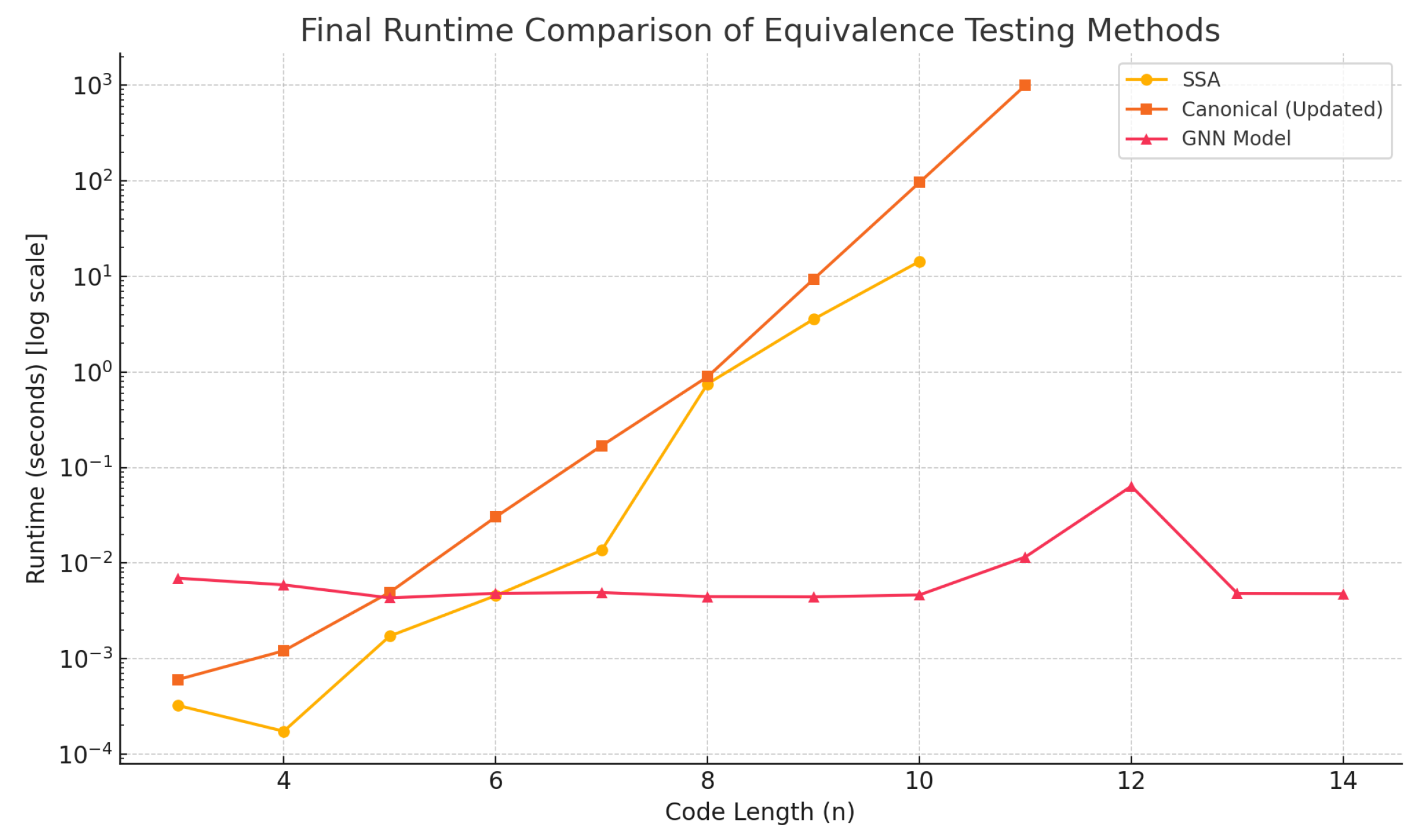

Table 1.
Average classification metrics across 5 test runs.
| Class | Precision | Recall | F1-Score |
|---|---|---|---|
| Not Equivalent | 0.996 | 0.996 | 0.996 |
| Equivalent | 0.995 | 0.998 | 0.996 |
| Accuracy | 0.996 | ||
Table 2.
Runtime Comparison of Equivalence Testing Methods.
| Code Length n | SSA (s) | Canonical (s) | GNN Model (s) |
|---|---|---|---|
| 3 | 0.000324 | 0.000604 | 0.006953 |
| 4 | 0.000174 | 0.001209 | 0.005919 |
| 5 | 0.001724 | 0.004948 | 0.004325 |
| 6 | 0.004569 | 0.030385 | 0.004825 |
| 7 | 0.013600 | 0.169057 | 0.004924 |
| 8 | 0.750951 | 0.892261 | 0.004461 |
| 9 | 3.561280 | 9.339438 | 0.004437 |
| 10 | 14.345400 | 96.203083 | 0.004643 |
| 11 | – | 1000.888818 | 0.011592 |
| 12 | – | – | 0.063821 |
| 13 | – | – | 0.004823 |
| 14 | – | – | 0.004787 |
Disclaimer/Publisher’s Note: The statements, opinions and data contained in all publications are solely those of the individual author(s) and contributor(s) and not of MDPI and/or the editor(s). MDPI and/or the editor(s) disclaim responsibility for any injury to people or property resulting from any ideas, methods, instructions or products referred to in the content. |
© 2025 by the authors. Licensee MDPI, Basel, Switzerland. This article is an open access article distributed under the terms and conditions of the Creative Commons Attribution (CC BY) license (http://creativecommons.org/licenses/by/4.0/).
Copyright: This open access article is published under a Creative Commons CC BY 4.0 license, which permit the free download, distribution, and reuse, provided that the author and preprint are cited in any reuse.


