Submitted:
29 September 2025
Posted:
30 September 2025
You are already at the latest version
Abstract
Effective integration of photovoltaic (PV) systems into electric power grids presents significant challenges due to the inherent variability of solar energy. Therefore, accurate PV power forecasting in various timescales is critical for the reliable operation of modern electric power systems. For short-term horizons, the primary source of solar power stochasticity is cloud movement and deformation, which are typically captured at high spatiotemporal resolutions using ground-based sky images. In this paper, we propose a novel multi-step sky image prediction framework for improved cloud tracking and short-term PV power forecasting. The proposed method is based on deep learning, but instead of being purely data-driven, we propose a hybrid approach where we combine Auto-Encoder-like Convolutional Neural Networks (AE-like CNNs) with physics-based sky image clustering, to enhance robustness towards fast-varying sky conditions and effectively model non-linearities without adding to the computational overhead. The proposed method is compared against several state-of-the-art approaches using a real-world case study comprising minutely sky images. Experimental results show improvements of up to 17.97% on structural similarity and 62.14% on mean squared error, compared to baseline approaches. These findings demonstrate that by combining effective physics-informed preprocessing with deep learning, multi-step ahead sky image forecasting can be reliably achieved even at low temporal resolutions.
Keywords:
ground-based sky images
; multi-step forecasting
; convolutional neural networks
; image classification
; photovoltaic generation
1. Introduction
In recent decades, Renewable Energy Sources (RES) have globally penetrated the Electric Power System (EPS), as they offer a wide range of advantages in the evolving energy landscape. RES are inexhaustible sources of environmentally friendly energy that contribute to reducing dependence on conventional generation units. Among them, solar energy stands out as the most abundant and globally accessible resource [1]. One of the primary applications of solar energy is photovoltaic (PV) power systems, which use PV cells to convert solar radiation into electric power. PV systems are considered highly trustworthy and offer considerable flexibility in installation, a decreasing cost over time (a 26% reduction in cost per unit of nominal capacity over the last decade, and a total reduction of 90% since 2000) [2] and an increasing average efficiency (through the introduction of advanced materials such as perovskite and technologies like tandem PVs) [3-4]. However, PV power generation is characterized by high variability that is primarily attributed to cloud movement, which undermines its reliability.
In the context of increasing the integration of PV generation into the EPS while simultaneously maintaining system reliability, significant attention has been directed towards PV power forecasting. PV power forecasting is utilized in a wide range of applications across various spatial and temporal scales, and its accuracy can significantly impact the stability of the EPS. PV power forecasting also brings value to all stakeholders within the electricity market. For power system operators, it facilitates congestion management and the extraction of operational flexibility. Energy producers benefit through improved participation in electricity and balancing markets, while also minimizing the risk of penalties. Finally, forecasting is advantageous for prosumers—individuals who both consume and produce electricity—by enabling more effective management of household energy loads [5].
Depending on the forecasting horizon, PV power forecasts are typically categorized into day-ahead, intra-day, and intra-hour forecasts [6]. This paper focuses on intra-hour forecasting, as it is critically important for the safe and economically efficient operation of EPS. Intra-hour minute-scale forecasting plays a key role in various applications, such as ramp-rate control, optimal management of energy storage systems, and real-time demand response [5].
A widely adopted approach for intra-hour PV power forecasting involves the use of ground-based sky images. Compared to numerical data alone, sky images provide significantly richer information regarding the presence and movement of clouds [7]. PV power forecasting based on sky images can be classified into two categories. The first group of methods directly translates sky images into PV power output using deep learning techniques [8-9]. The second group introduces an intermediate stage, in which cloud motion is modeled and future sky conditions are predicted before being translated into PV generation [10]. Compared with the first group of methods, motion-based approaches have the advantage of establishing a clearer physical link between cloud dynamics and PV variability, while also improving the robustness of forecasts under rapidly changing sky conditions [11].
Methods for modeling cloud motion in solar forecasting can be grouped into Cloud Motion Vector (CMV)-based methods [12-14] and Artificial Intelligence (AI) approaches [10]. CMV-based methods, including Optical Flow (OF) and Block Matching (BM) algorithms, are computationally efficient and interpretable but struggle with rapidly evolving or overlapping clouds because they assume linear cloud motion. This linearity assumption limits the forecasting horizon and imposes the requirement for high temporal resolution in the input imagery. AI-based approaches, such as Convolutional Neural Networks (CNNs), capture nonlinear spatiotemporal patterns and enhance robustness under variable conditions; however, they typically require deeper architectures to avoid premature convergence to local optima, demanding large datasets for training and substantial computational resources [11], which makes them impractical for local smart microgrids. A summary of CMV-based and AI-based Cloud Motion Modeling (CMM) methods used in solar forecasting is provided in Section 2.
This paper proposes a novel multi-step sky image prediction model, for minute-scale PV power forecasting. Unlike previous methods, the proposed hybrid approach combines physics-informed data pre-processing with deep learning, to effectively capture non-linearities of cloud dynamics without requiring excessive computational resources. To this end, a dataset of sky images was classified into clusters using a recently-proposed method based on unsupervised learning and hybrid image feature representation, and cluster-specific CNNs trained to forecast sequences of sky images. The key contributions of this paper are summarized as follows:
- The combination of Auto-Encoder (AE)-like CNNs with a physics-informed data preprocessing pipeline primarily focusing on input classification. The proposed model simplifies the original forecasting problem by decomposing it into simpler subproblems comprising more homogeneous data. This approach lowers the risk of premature convergence to suboptimal solutions, and thus decreases training data requirements and enhances the generalization capability of the AE-like CNNs;
- A sensitivity analysis is separately conducted for each cluster. The optimal kernel size and number of hidden layers are separately determined for the AE-like CNN associated with each cluster, rather than being universally fixed across all clusters. This per-cluster sensitivity analysis allows for optimal adaptation to the specific characteristics of each sky condition and further reduces the risk of premature convergence;
The remainder of this paper is organized as follows: In Section 2, a brief overview of the related literature is provided. In Section 3, the methodology of the proposed sky image forecasting framework is presented along with the fundamental theoretical background. Details of the experimental setup and the proposed prediction process are provided in Section 4. Section 5 presents and discusses the experimental results. The main conclusions are summarized in Section 6.
2. Related Work
For several years, sky image forecasting typically relied on physics-based CMM techniques to extract CMVs and extrapolate the future position of clouds. A comprehensive survey of CMV-based methods can be found in [15]. Commonly used CMM techniques for sky images include OF [12], BM [13], and Particle Image Velocimetry (PIV) [14]. These methods generally rely on linear motion assumptions and thus fail to capture the non-linear nature of cloud dynamics, such as cloud deformation and displacement [16]. Moreover, traditional CMV-based methods assume brightness consistency between consecutive images, making them prone to errors induced by reflections, noise, and the low resolution of cheap camera systems. These limitations constrain the forecasting horizon [17] and necessitate sky images to be captured at high temporal resolutions, which is not always feasible in practice.
Various efforts have been made to overcome the challenges of traditional CMV-based methods. A novel 3D CMM approach leveraging a network of All-Sky Imagers (ASIs) was introduced in [18]. In [19], several modifications to the sector ladder method were introduced to address periods of high intermittency and enable real-time irradiance forecasting. In [20], a CMV-based technique incorporating image-phase-shift invariance and Fourier phase correlation theory was developed for improved cloud displacement estimation and short-term PV power forecasting. While these methods managed to improve cloud displacement forecasting accuracy, they remain constrained by the inherent linear assumptions of traditional CMV-based methods, particularly under highly variable sky conditions and coarser temporal resolutions.
In [16], OF and BM approaches were linearly combined with a feature matching method into an ensemble model, with weights determined using Particle Swarm Optimization (PSO). The model was separately calibrated for each of the sky image classes generated using k-Means clustering on features extracted from Gray Level Co-occurrence Matrices (GLCM). The ensemble method consistently outperformed the standalone approaches, highlighting the effectiveness of combining complementary techniques. Furthermore, the classification of input images played a crucial role in improving accuracy, as it allowed the ensemble to be tailored to distinct sky conditions. However, the ensemble model still exhibited relatively high errors in some of the more challenging classes, likely due to the inherent linear nature of the ensemble combination and the coarse temporal resolution of the sky images. Moreover, finetuning the hyperparameters of each standalone model of the ensemble remains a challenging task—particularly when finetuning is done separately for each cluster.
The rapid advancement of AI in recent years has driven widespread adoption of deep learning techniques in computer vision applications. Inspired by video prediction models, [10] utilized AE-like CNNs for sequential sky image prediction based on previous image sequences. Unlike CMV-based methods, this approach demonstrated greater robustness to noise and coarser temporal resolutions. Other studies have bypassed sky image forecasting altogether, directly predicting PV generation from sky images through deep end-to-end CNN-based (Deep Neural Networks – DNN) models. For example, [8] developed several end-to-end models, with those leveraging sequences of sky images as input outperforming others under more dynamic conditions. In [9], ECLIPSE was proposed for the joint prediction of segmented sky images or satellite images alongside associated irradiance values.
Although DNN methods effectively capture local non-linear cloud dynamics, they exhibit limitations. Optimization via backpropagation-based gradient descent is prone to local optima entrapment, often resulting in premature convergence and sub-optimal model calibration, particularly in complex scenarios with highly non-convex objective spaces, such as those encountered in minute-scale PV generation forecasting [21]. In addition, the inherent locality of convolutional filters restricts their ability to capture the global structure of sky images, impairing cloud tracking performance under highly dynamic sky conditions [22]. Furthermore, the pure data-driven DNN architectures depend heavily on historical datasets, limiting their generalization capability to sky conditions with low mutual information to the training data. To mitigate these limitations, deep generative AI models have recently attracted growing interest. In [22], an end-to-end multi-modal model utilizing Vision Transformers (ViTs) was proposed for short-term irradiance forecasting. Acknowledging the limitations of end-to-end modeling for cloud tracking, [17] introduced a two-step approach for PV power forecasting, combining a U-net model with SkyGPT, a deep generative AI model for stochastic sky image sequence prediction. While deep generative AI models help address part of the shortcomings of DNN approaches, they still rely on backpropagation-based gradient descent optimization algorithms and demand large datasets and extensive training on resource-intensive platforms, significantly increasing computational requirements. To alleviate this, in this paper we propose a hybrid approach that deviates from the pure data-driven paradigm.
3. Methodology
3.1. Forecasting Framework
In the present work, the forecasting framework consists of multi-step sky image prediction. The whole concept is to create a model that takes a sequence of n consecutive sky images and returns a sequence of the next m sky images (Figure 1). In Figure 1, is the time of the forecast issuing, is the sky image at , S is the sky image sequence used as input, and S’ is the forecasted sky image sequence.
3.2. Auto Encoder-like Convolutional Neural Networks
The sky image prediction model in this paper employs AE-like CNNs. CNNs are feed-forward artificial neural networks that contain convolutional layers. They are widely used in computer vision, due to their capability of extracting features and patterns from images, using linear algebra methods [23]. The employed CNN imitates the structure of an AE (Figure 2). It contains an encoder (takes the input images and compresses them into a latent vector), a bottleneck layer (the encoded information) and a decoder (decompresses the encoded information into a new set of images). This process can be mathematically modeled through the following relation:
where S is the input sky image sequence, S’ is the forecasted sky image sequence and , are the decoding and encoding mapping functions, respectively. The encoder and the bottleneck layer use convolutional layers, while the decoder uses transposed convolutional layers [24].
In the proposed AE-like CNN, the output of each layer is calculated using the following procedure: At first, the previous layer is multiplied with the corresponding weights, and a bias matrix is added. Then, Batch Normalization (BN) and activation are applied, giving the output values of the layer [10]. Τhe architecture of the proposed AE-like CNN is shown in Figure 3.
The AE-like CNN models are trained to extract the input-output relationship. For this purpose, an early stopping mechanism is included, which halts training if no improvement is observed in the validation error for N consecutive epochs (where N is defined by a patience parameter) to prevent overfitting.
3.3. 2D and 3D Convolutions
The proposed sky image prediction model was implemented using two types of convolutions. The first one is the 2D convolution, in which a 2D filter is applied to each image of the sequence simultaneously, and the result is a 2D output frame. For K filters, the outcome of each convolution layer is K 2D output frames:
The 2D convolution is illustrated in Figure 4a.
Input (H1×W1×L) → Output (H2×W2×K)
The second one is the 3D convolution, in which a 3D filter is used instead. The outcome is a 3D output volume for each filter (Figure 4b):
In (2) and (3), H1×W1 are the dimensions of the input frames, H2×W2 are the dimensions of the output frames, L the length of the input sequence, is the length of the output volume, K is the number of filters used per layer and f is the size of the filters [10]. can be calculated as follows:
Input (H1×W1×L) → Output (H2×W2×L’×K)
3.4. Data Preprocessing
Sky images are typically captured at high resolutions in color (RGB images). Consequently, each image has 3 channels of H1×W1 pixels. The number of operations per convolution is proportional to the dimensions of the image; thus, it is evident that retaining the original image dimensions is computationally impractical. Moreover, raw data handling potentially enables the extraction of even more information from the source data, but it makes getting stuck in local optima even more likely. That occurs because the backpropagation algorithm is not subserved by any known information or correlation about the signals. Therefore, all images undergo a preprocessing pipeline that includes conversion to grayscale, resolution downscaling, and classification.
3.4.1. Grayscaling
The first stage of sky image preprocessing involves conversion to grayscale, by reducing the number of channels per image from three (RGB) to one. This step decreases the computational load while preserving the essential information required for recognition of objects, such as the sun and cloud distribution—both critical for future sky image prediction. The grayscale conversion was performed according to the following equation:
where , , are the values of the i-th pixel in the red, green and blue channels, respectively, of the original image and is the value of the i-th pixel of the new image.
3.4.2. Downscaling
The downscaling preprocessing step is essential, as it significantly decreases the number of pixels per image, thereby reducing the number of convolutions and the total training time. Importantly, this resolution reduction does not compromise the ability to recognize the key visual elements (i.e., clouds and the sun). To downscale the sky images, the value of each new pixel is computed as the average of the original pixels within its corresponding region:
where is the value of the new (downscaled) pixel , the value of each original pixel that falls within the region of the new pixel , and is the number of original pixels that fall within that region. This downscaling approach corresponds to an average pooling operation. Compared to nearest neighbor interpolation, this method avoids aliasing artifacts, and compared to bilinear or bicubic interpolation, it is computationally simpler while still maintaining the key spatial patterns necessary for sky condition recognition [25].
3.4.3. Classification of the Input Data
In this paper the input data are passed through a classification process; thus, the sky images are divided into clusters of similar sky conditions. Classification is a technique that helps reduce the impact of dataset imbalance and the variability of the dataset by creating more coherent subsets. For each cluster, a class-specific sky image forecasting model is separately trained. Hence, the original problem is decomposed into smaller and simpler subproblems, since trainings take place with more homogeneous data. This is especially crucial because when less non-linearity and non-homogeneity is observed, the hill climbing requirement during optimization reduces and the chances of the gradient-descent backpropagation algorithm to find the “global optimum” increases significantly.
The employed sky image classification approach is a recently proposed automatic method based on unsupervised learning and downstream evaluation [26]. A schematic overview of the employed approach is provided in Figure 5. A wide range of global spectral and textural handcrafted features is extracted from multiple color spaces of each sky image to capture tonal variations and color distributions. Additional handcrafted features related to the total cloud coverage, cloud velocity, and solar elevation are incorporated to account for PV energy yield variations. The handcrafted features are encoded using a hybrid dimensionality reduction technique that combines Principal Component Analysis (PCA) and shallow, fully-connected feed-forward AEs. The resulting latent feature set is then clustered using k-Means clustering. The optimal number of clusters is identified through a novel forecast-driven strategy, which co-optimizes k with a minute-scale PV energy yield forecasting model – leveraging PV generation data associated with the sky images – and subsequent downstream evaluation. More details on the employed sky image classification approach can be found in [26].
The employed sky image classification method is primarily selected for its ability to extract multi-class partitions without relying on pre-assigned ground-truth labels [26]. This eliminates the need for manual labeling, enhancing both the practicality and scalability of the classification process. Furthermore, determining the number of clusters with respect to the minimization of the average forecasting error of the downstream PV model results in more detailed partitions than those typically achieved using standard clustering metrics based on cohesion and separation. This is particularly relevant as sky image classification involves fine-grained distinctions where instances are not easily separable [26]. Unlike [26], in which the sky image classification was used for minute-scale PV energy yield forecasting, here the classification is conducted for minute-scale sky image sequence prediction; therefore, sky images closer to dusk and dawn are included in the training dataset. In contrast to self-supervised learning methods based on DNNs, the employed approach extracts global features from the sky images that facilitate the identification of subtle distinctions and fine-grained classification. Unlike similar unsupervised learning methods, the employed approach incorporates non-instantaneous features to the original handcrafted feature set, e.g., CMV and solar elevation variations, creating a form of physics-informed machine learning approach that improves performance and reduces the computational requirements [26]. These variations are obviously related to cloud movement and should thus be considered when classifying the input for sky image forecasting.
4. Experimental Setup
4.1. Data Presentation and Analysis
In this study, ground-based sky images were utilized, captured over a 14-day period (from 16/11/2023 to 29/11/2023), in a timespan from sunrise to sunset, with a temporal resolution of one frame per minute and finally 8168 images were acquired [26]. Data were collected near a PV system with an installed capacity of 1.2 kW, located in the region of Boeotia, Greece. Although the dataset pertains to a mild arid climate, the dataset is quite diverse (32% sunny, 22% cloudy and 46% overcast). The images were captured using an EKO ASI-16 sky monitoring camera manufactured by CMS Ing. Dr. Schreder GmbH. The camera features a 180° field of view, 5 MP resolution, and a wide-angle fisheye lens, enclosed within a reflective and durable quartz dome equipped with an air circulation system to prevent fogging. All images were captured in color (Red, Green, and Blue − RGB) and stored in JPG format, with an average file size of 76.52 KB. To ensure the validity of the results, the image acquisition location was carefully selected to minimize noise from external obstructions (e.g., buildings, trees).
4.2. Classification Results
According to the classification method that was described in Section 3.4., the whole dataset was divided into eight clusters that correspond to eight different sky conditions:
- Overcast (936 sequences);
- Sunny (1963 sequences);
- Clear sky and the sun near to sunset (561 sequences);
- Almost overcast (1442 sequences);
- Clear sky and the sun at sunrise (794 sequences);
- Sun low on the horizon and partial cloud cover (517 sequences);
- Partial cloud cover with thin clouds (885 sequences);
- Partial cloud cover with thick clouds (753 sequences).
Figure 6 presents representative examples of sky images contained in each cluster.
4.3. Proposed Prediction Process
Out of the eight clusters, some demonstrate considerable variability, while others present slighter changes. For example, clusters (1), (4), (6), (7) and (8) are associated with relatively high cloud coverage and thus intense cloud motion on an intra-minute scale, in contrast to clusters (2), (3) and (5), where the sky is almost clear. Thus, while AE-like CNN models are required for the former clusters to capture their inherent variability, the persistence method can be used for the latter, to decrease the overall computational load. Persistence is a method that assumes that the future values of a random variable are the same as the present ones (worst case scenario) and performs well for short-term forecasting horizons and decreased variability.
The prediction process begins with the classification of the current sky image into a suitable cluster, according to the classification method that is thoroughly described in Section 3.4.3 [26]. Afterwards, if the cluster belongs to the first category (high variability), the associated trained AE-like CNN model is called; otherwise, the persistence method is used instead. Then, the prediction implementation takes place and finally the future sky image sequence is extracted. The flow chart of the proposed sky image prediction process is illustrated in Figure 7.
4.4. Configuration Setup
4.4.1. Data Organization
In this paper, the forecasting horizon is set to 10 minutes, with a forecasting resolution of 1 minute. Τhe sky image prediction model takes a sequence of ten input sky images and returns a sequence of ten forecasted sky images. The forecasting procedure can be mathematically formulated as follows:
where I refers to a sky image, and are the temporal resolutions of the input and output sequence, respectively (, is the time of forecasting issuing, is the input sequence length (), and is the forecasting horizon (). For this purpose, the preprocessed data are organized in batches of 20 consecutive images of which the first 10 represent the input and the last 10 represent the output. In total, 7851 sequences were obtained and got split into training, validation and test sets with a ratio of 70%, 15%, and 15%, respectively.
4.4.2. Model’s Architectures, Implementation Details, and Environment
Τhe proposed AE-like CNN models were implemented using 2D and 3D Convolutions, with 3, 5, 7, 9 and 11 hidden layers and 32×32, 64×64 input images dimensions.
The number of filters and output frame dimensions per layer were chosen according to [10]. Epochs and patience values (mentioned in Section 3.2) were set to 100 and 10, respectively, and were selected empirically after a series of tests, aiming to maintain model accuracy while also limiting training time and computational cost. The optimization algorithm chosen for the training process was Adam optimization, with the learning rate set to 0.001.
All models were implemented in Python, using the Spyder environment and the TensorFlow–Keras library. The computational system used was an 11th Gen Intel® Core™ i5-1135G7 @ 2.40GHz 2.42 GHz laptop computer, with 8.00 GB of RAM.
5. Results
5.1. Assessment Metrics
To evaluate the performance and estimate the average error of the sky image prediction models, a comparison between the predicted images and the target (ground-truth) images is required. This comparison is achieved using quantitative evaluation metrics. In the case of sky images, commonly employed metrics include the Mean Squared Error (MSE) and the Structural Similarity Index Measure (SSIM) [10].
5.1.1. Mean Squared Error
MSE compares two images pixel by pixel based on their intensity values. MSE is computed as follows [27]:
where x is the predicted image, y is the target image, (i, j) are the pixel coordinates, and M, N are the image dimensions. The smaller the MSE value, the more similar the two images are.
5.1.2. Structural Similarity Index Measure
SSIM quantifies the degree of similarity between two images. It depends on the following three factors [28]:
- Luminance: A measure of the brightness difference of the two images;
- Contrast: A contrast comparison (i.e., the difference between bright and dark regions within the image) between the two images;
- Structure: An estimation of the spatial arrangement of luminance patterns within the images;
The mathematical formulation of SSIM between two images is presented through equations (9) to (13):
where x the predicted image, y the target image, the luminance term, the contrast term, the structural term, and the mean pixel values of images x and y, respectively, and the standard deviation of the pixel values of images x and y, respectively, the covariance of the pixel values of images x and y, and , , constants added to avoid division by values close to zero in the denominator of the terms. In this paper, we select the values suggested in [10], i.e., , , , and . Unlike MSE, the higher the SSIM value, the more similar the two images are.
5.2. Benchmark Forecasting Models
The following benchmark methods are developed for comparison with the proposed 8-Cluster AE-like CNN sky image prediction model:
- Persistence;
- CMV-based method;
- 1-Cluster AE-like CNN;
- 3-Cluster AE-like CNNs;
- 6-Cluster AE-like CNNs.
5.2.1. Persistence Method
The persistence method supposes no further change in a random variable’s value. If is the sky image at , then the prediction for will be:
where k is any timestep in the forecasting horizon.
5.2.2. CMV-based Method
The CMV-based benchmark is based on the Gunnar Farneback OF method [29]. This method compares the pixel intensities between two consecutive sky images to extract a dense CMV field, which is then used to linearly extrapolate future cloud movement. The Gunnar Farneback OF method has been widely used for CMM from sky images, both as a standalone method and in combination with other approaches [30].
5.2.3. AE-like CNN
Apart from the proposed 8-Cluster AE-like CNN model, similar AE-like CNN models with 3 and 6 clusters were developed according to the procedure that was thoroughly described in Section 3 and Section 4, to assess the impact of the number of clusters on the forecasting performance. In addition, a 1-Cluster AE-like CNN, trained on the entire dataset, was included to assess the model’s generalization capability when using all available data.
5.3. Sensitivity Analysis
As mentioned in Section 4.3, the proposed 8-Cluster sky image prediction model uses AE-like CNNs for the clusters that are associated with sky conditions of intense variability and the persistence method for the rest of the clusters. In order to find the optimum combination of hyperparameters for which the AE-like CNNs perform better, a sensitivity analysis was conducted. The hyperparameters to be finetuned were: the convolution type (CT), the kernel size (KS), the number of hidden layers (NHL) and the input image dimensions (IID). The complete set of experiments is presented by the following Cartesian product:
Preliminary tests showed that in cases where CT was 3D and IID was 64, the AE-like CNNs exhibited worse performance and a significantly longer training time. For this reason, and to reduce the overall evaluations and computational overhead, CT=2D and IID=32 were pre-selected, and the sensitivity analysis continued for KS and NHL. The simplified Cartesian product is now as follows:
This simplification makes the implementation of a per-cluster sensitivity analysis computationally feasible. Thus, each cluster sets its own cluster-specific hyperparameters values that correspond to the particular sky condition. The per-cluster sensitivity analysis results for each of the eight clusters of the proposed model is shown in Table 1. The optimum combination of KS and NHL for each cluster is in bold. As can be seen, the model’s performance is highly affected by changes in hyperparameter values. In many cases, premature convergence can be noticed, causing a significant deterioration in the assessment metrics values.
From the sensitivity analysis results it can be concluded that for KS = 3 the kernels are too small, resulting in overly local feature extraction, while AE-like CNNs require at least 9 layers to adequately model the input–output relationship. In general, KS = 5 and NHL = 9 or 11 yield the best results for most clusters.
5.4. Final Forecasting Results
Table 2 shows the final values of the assessment metrics for each sky image forecasting model that was implemented. The results for the 3-Cluster AE-like CNN, the 6-Cluster AE-like CNN, and the proposed 8-Cluster AE-like CNN are aggregated across all clusters. From Table 2 it can be seen that all AE-like CNN models perform better compared to the persistence method, with the proposed 8-Cluster model yielding the best results. The OF model achieves an improvement of 13.68% on SSIM and a deterioration of 21.32% on MSE, compared to persistence. This performance deterioration is likely due to the limitations of OF in coarser temporal resolutions. In the case of the model without classification, although the evaluation metrics indicate satisfactory similarity between the images, visual inspection highlights the need for improved results. The output image sequences suggested that the model responded adequately under clear-sky conditions, as it successfully identified the sun’s position and captured image brightness to a reasonably good extent. However, under cloudy conditions, although the sun’s location is detected, the model fails to accurately predict cloud distribution. These observations indicate that, for image-based forecasting tasks, relying solely on quantitative metrics is inadequate, as such measures treat images merely as numerical arrays and may overlook perceptual differences. Thus, complementing quantitative assessment with qualitative (visual) evaluation is essential to obtain a more complete understanding of model performance.
The performance of the AE-like CNN models improves significantly with the increase in the number of clusters, reaching improvements of 73.1% and 24.3% on MSE and SSIM, respectively, compared to persistence. Based on this observation, it can be concluded that the AΕ-like CNN model performs better —becoming more capable of recognizing patterns— when it is trained on more homogeneous image subsets. From Table 2, it seems that from the 6-Cluster model to the 8-Cluster model the improvements are quite imperceptible (0.86% and 7.02% on SSIM and MSE respectively), showing that further classification is unnecessary. This saturation was expected to occur at some point, as beyond a certain level, the subproblems become sufficiently simple and the data highly homogeneous, allowing the AE-like CNN to handle them effectively without the risk of getting trapped in a local optimum. The proposed model was selected to be the 8-Cluster, as it appears to be the “knee point” beyond which the additional accuracy gain is not worth the investment of more effort.
As far as training time is concerned, it seemed to decline with the increase in the number of clusters. Specifically, in our relatively low capability computer system (described in Section 4.4.2) that we executed our simulations, the model without classification required approximately 26.75 hours for training, whereas the proposed 8-Cluster required approximately 16.6 hours of total training time, a significant reduction of 37.94%. This training time reduction may be attributed to several reasons, such as the reduced per-epoch training time from the smaller data subsets of each cluster and the overall fewer epochs required for convergence due to more homogeneous clusters that create simpler sub-problems.
Table 3 presents the results per cluster for the proposed model. Overall, each cluster achieved strong performance, with notably low MSE values and SSIM values exceeding 90%, indicating strong correlation between real and predicted sequences. Clusters 1 and 6 achieved the best MSE (0.0155%) and SSIM (98.5%) values, respectively. Persistence demonstrated sufficient accuracy for the chosen clusters that are associated with sky conditions of mild variability, combining effectiveness and low computational cost.
In Figure 8 and Figure 9, examples of generated sky image forecasts are depicted for clusters 6 and 8, respectively. For each figure, the first row illustrates the real sequence, the second row the forecasted one and the third is a heat map that visualizes the MSE for each pixel between the two images. In these two examined cases, different color bar scales are applied to the heat maps to ensure that the variations in error are clearly distinguishable. Comparing the forecasted sky images to the real ones, it is obvious that the cloud distribution and coverage ratio have been accurately modeled, and the model has also correctly predicted whether the sun is blocked or not. Even in the case of Cluster 8, where more pronounced variations are present, the model was able to predict them with high accuracy. By observing the heat maps, it becomes clear that the model has achieved its objective, since the heat maps are mostly white — indicating low MSE values—with a few isolated red patches that reveal localized error spikes.
The per-cluster sensitivity analysis is a major factor in the performance of the proposed sky image prediction model. If a predetermined set of hyperparameters, derived from a sensitivity analysis on the entire dataset, is applied instead, the results of the proposed 8-Cluster model would be considerably worse. To demonstrate this, the AE-like CNNs of all clusters are trained using KS=3 and NHL=5, as suggested in [10], and the results are compared to those obtained from the cluster-specific sensitivity analysis. Table 4 presents this comparison.
With the use of the per-cluster sensitivity analysis, MSE and SSIM are improved by 61.87% and 12.97%, respectively. That happens because each cluster addresses a different subproblem of cloud motion and thus its corresponding prediction model requires a specific configuration to adapt to the characteristics of the sky image cluster.
5.5. Alternative Dataset Split
In order to examine the models’ capability in a different dataset split, all experiments were repeated for a split that uses 50% on training set, 25% on validation set and 25% on test set. This split was chosen as a more balanced option between training and validation and to evaluate the robustness of the proposed approach toward limited training data availability. The results are depicted in Table 5.
When compared with the 1-cluster model, the benefit of clustering remains clear, while the 3-Cluster model even shows an improvement in the alternative split, suggesting better generalization with fewer training samples. On the other hand, the 6-Cluster model performs notably worse, as the division into six groups does not secure stable training; in some clusters the model converged prematurely, leading to weak overall results. The proposed 8-Cluster model proves the most consistent, with only slight differences observed across the two splits. This indicates that the approach remains effective even when the amount of training data is reduced.
6. Conclusions
This paper proposes a multi-step forecasting framework for predicting sequences of ground-based sky images. The proposed approach has combined physics-informed clustering of images and AE-like CNN models, which have been trained separately for each cluster. In addition, a per-cluster sensitivity analysis has been conducted, allowing the model to adapt better to the specific characteristics of each cluster and the rapidly changing sky conditions. The evaluation on a real-world sky image dataset has demonstrated clear gains over baseline approaches, both in terms of SSIM and MSE. Dividing the forecasting task into smaller and more homogeneous groups of data has simplified the learning process, reduced training effort, and allowed the CNNs to capture the underlying patterns more effectively, thereby improving their generalization capability. The per-cluster sensitivity analysis has further improved the results by up to 61.87% in terms of MSE. Moreover, the proposed approach has exhibited robustness toward limited training data, which is particularly important for distributed local PV systems with limited historical data availability. These results confirm that physics-informed preprocessing, together with targeted hyperparameter tuning, can make multi-step ahead sky image forecasting feasible even when the available data have relatively low temporal resolution, without the need for excessive computational resources and long training datasets. Apart from the numerical gains, the findings underline the practical importance of careful data preparation when forecasts need to cope with highly variable sky conditions.
References
- Chow, S.K.H.; Lee, E.W.M.; Li, D.H.W. Short-term prediction of photovoltaic energy generation by intelligent approach. Energy Build. 2012, 55, 660–667. [CrossRef]
- Solar Panel Prices Over Time. Available online: https://www.cladco.co.uk/blog/post/solar-panel-prices-over-time (accessed on 23 September 2025).
- Snaith, H.J. Present status and future prospects of perovskite photovoltaics. Nat. Mater. 2018, 17, 372–376. [CrossRef]
- Martinho, F. Challenges for the future of tandem photovoltaics on the path to terawatt levels: a technology review. Energy Environ. Sci. 2021, 14, 3840–3871. [CrossRef]
- Sengupta, M.; Habte, A.; Wilbert, S.; Gueymard, C.; Remund, J.; Lorenz, E.; van Sark, W.; Jensen, A.R. Best Practices Handbook for the Collection and Use of Solar Resource Data for Solar Energy Applications, 4th ed.; 2024.
- Diagne, M.; David, M.; Lauret, P.; Boland, J.; Schmutz, N. Review of solar irradiance forecasting methods and a proposition for small-scale insular grids. Renew. Sustain. Energy Rev. 2013, 27, 65–76. [CrossRef]
- Barbieri, F.; Rajakaruna, S.; Ghosh, A. Very short-term photovoltaic power forecasting with cloud modeling: A review. Renew. Sustain. Energy Rev. 2017, 75, 242–263. [CrossRef]
- Kong, W.; Jia, Y.; Dong, Z.Y.; Meng, K.; Chai, S. Hybrid approaches based on deep whole-sky-image learning to photovoltaic generation forecasting. Appl. Energy 2020, 280, 115875. [CrossRef]
- Paletta, Q.; Hu, A.; Arbod, G.; Lasenby, J. ECLIPSE: Envisioning cloud induced perturbations in solar energy. Appl. Energy 2022, 326, 119924. [CrossRef]
- Fu, Y.; Chai, H.; Zhen, Z.; Wang, F.; Xu, X.; Li, K.; Shafie-Khah, M.; Dehghanian, P.; Catalão, J.P.S. Sky image prediction model based on convolutional auto-encoder for minutely solar PV power forecasting. IEEE Trans. Ind. Appl. 2021, 57, 3272–3281. [CrossRef]
- Lin, F.; Zhang, Y.; Wang, J. Recent advances in intra-hour solar forecasting: A review of ground-based sky image methods. Int. J. Forecast. 2023, 39, 244–265. [CrossRef]
- Wood-Bradley, P.; Zapata, J.; Pye, J. Cloud tracking with optical flow for short-term solar forecasting. In Proceedings of the 50th Conference of the Australian Solar Energy Society, Melbourne, Australia, 2012.
- Chow, C.W.; Urquhart, B.; Lave, M.; Dominguez, A.; Kleissl, J.; Shields, J.; Washom, B. Intra-hour forecasting with a total sky imager at the UC San Diego solar energy testbed. Sol. Energy 2011, 85, 2881–2893. [CrossRef]
- Marquez, R.; Coimbra, C.F.M. Intra-hour DNI forecasting based on cloud tracking image analysis. Sol. Energy 2013, 91, 327–336. [CrossRef]
- Sawant, M.; Shende, M.K.; Feijóo-Lorenzo, A.E.; Bokde, N.D. The state-of-the-art progress in cloud detection, identification, and tracking approaches: A systematic review. Energies 2021, 14, 8119. [CrossRef]
- Zhen, Z.; Pang, S.; Wang, F.; Li, K.; Li, Z.; Ren, H.; Shafie-Khah, M.; Catalão, J.P.S. Pattern classification and PSO optimal weights based sky images cloud motion speed calculation method for solar PV power forecasting. IEEE Trans. Ind. Appl. 2019, 55, 3331–3342. [CrossRef]
- Nie, Y.; Zelikman, E.; Scott, A.; Paletta, Q.; Brandt, A. Skygpt: Probabilistic ultra-short-term solar forecasting using synthetic sky images from physics-constrained videogpt. Adv. Appl. Energy 2024, 14, 100172. [CrossRef]
- Peng, Z.; Yu, D.; Huang, D.; Heiser, J.; Yoo, S.; Kalb, P. 3D cloud detection and tracking system for solar forecast using multiple sky imagers. Sol. Energy 2015, 118, 496–519. [CrossRef]
- Bone, V.; Pidgeon, J.; Kearney, M.; Veeraragavan, A. Intra-hour direct normal irradiance forecasting through adaptive clear-sky modelling and cloud tracking. Sol. Energy 2018, 159, 852–867. [CrossRef]
- Wang, F.; Zhen, Z.; Liu, C.; Mi, Z.; Hodge, B.-M.; Shafie-Khah, M.; Catalão, J.P.S. Image phase shift invariance based cloud motion displacement vector calculation method for ultra-short-term solar PV power forecasting. Energy Convers. Manag. 2018, 157, 123–135. [CrossRef]
- Kousounadis-Knousen, M.A.; Anagnostos, D.; Bazionis, I.K.; Bakovasilis, A.; Georgilakis, P.S.; Catthoor, F. Accurate PV Energy Yield Forecasting. In Energy Production, Load and Battery Management Framework with Supporting Methods for Smart Microgrids; Catthoor, F., et al., Eds.; Springer: Cham, Switzerland, 2025; pp. 25–46. https://doi.org/10.1007/978-3-031-92025-7_2.
- Liu, J.; Zang, H.; Cheng, L.; Ding, T.; Wei, Z.; Sun, G. A transformer-based multimodal-learning framework using sky images for ultra-short-term solar irradiance forecasting. Appl. Energy 2023, 342, 121160. [CrossRef]
- Zhang, A.; Lipton, Z.; Li, M.; Smola, A.; et al. Dive into deep learning. arXiv 2021, arXiv:2106.11342.
- Dumoulin, V.; Visin, F. A guide to convolution arithmetic for deep learning. arXiv 2018, arXiv:1603.07285.
- Gonzalez, R.C.; Woods, R.E. Digital Image Processing, 4th ed.; Pearson: London, UK, 2018.
- Kousounadis-Knousen, M.A.; Catthoor, F.; Bakovasilis, A.; Georgilakis, P.S. Automatic multiclass classification of unlabeled ground-based sky images for minute-scale PV energy yield forecasting. IEEE Access 2025, 13, 120547–120562. [CrossRef]
- Michael, N.E.; Suykens, J.A.K.; Deconinck, G.; De Vos, K. Short-Term Solar Power Predicting Model Based on Multi-Step CNN-Stacked LSTM Technique. Energies 2022, 15, 2150.
- Xu, F.; Sun, Y.; Guo, M. Prediction of Solar Flux Density Distribution Concentrated by a Heliostat Using a Ray Tracing-Assisted Generative Adversarial Neural Network. Energies 2025, 18, 1451. [CrossRef]
- Farnebäck, G. Two-frame motion estimation based on polynomial expansion. In Proceedings of the Scandinavian Conference on Image Analysis, Halmstad, Sweden, 29 June–2 July 2003; Springer: Berlin/Heidelberg, Germany, 2003; pp. 363–370. [CrossRef]
- Arrais, J.M.; Cerentini, A.; Martins, B.J.; Chaves, T.Z.L.; Neto, S.L.M.; von Wangenheim, A. Systematic Review on Ground-Based Cloud Tracking Methods for Photovoltaics Nowcasting. Am. J. Clim. Change 2024, 13, 452–476. [CrossRef]
Figure 1.
Sky image sequence prediction framework employed in this paper.
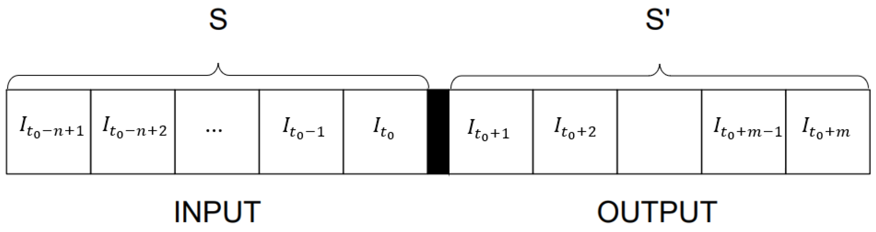
Figure 2.
The structure of a typical Auto Encoder.
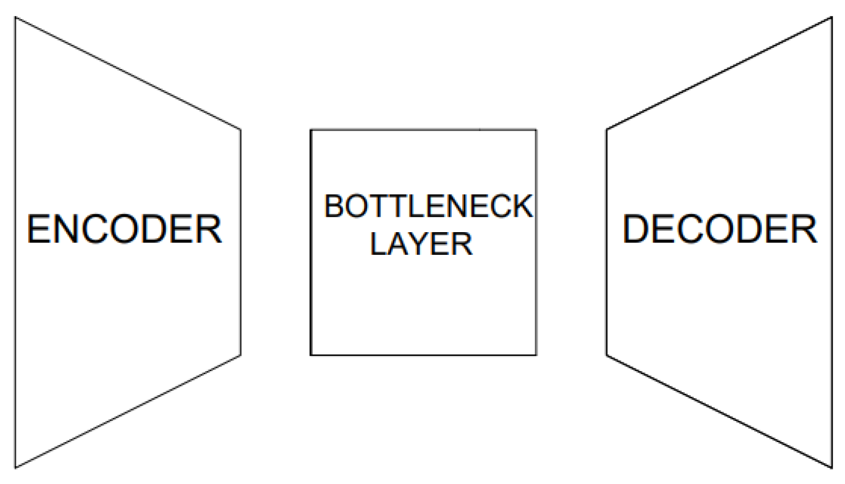
Figure 3.
Architecture of the proposed AE-like CNN.
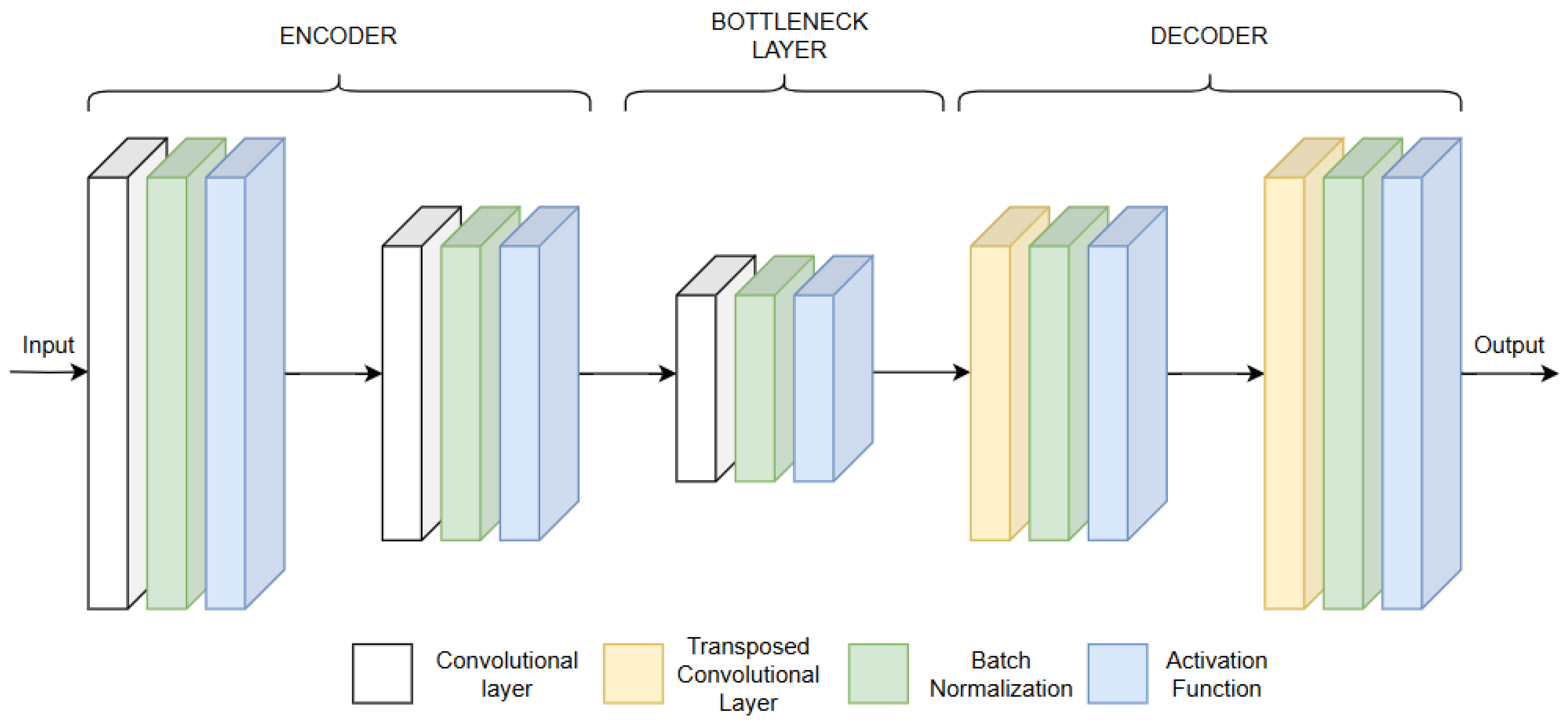
Figure 4.
Convolution types: (a) 2D Convolution (b) 3D Convolution.
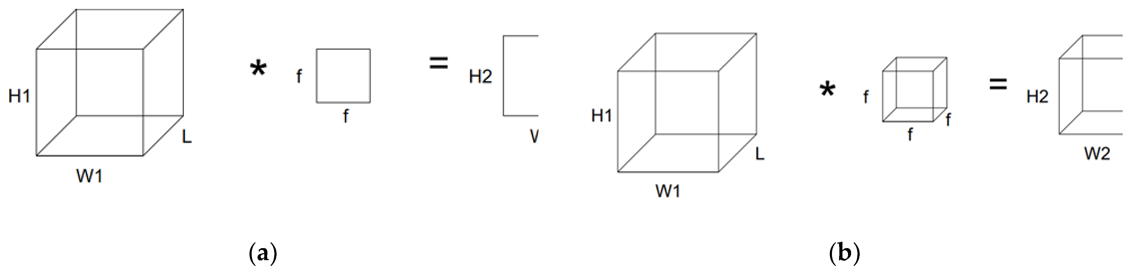
Figure 5.
Overview of the employed approach for the automatic classification of the sky images.
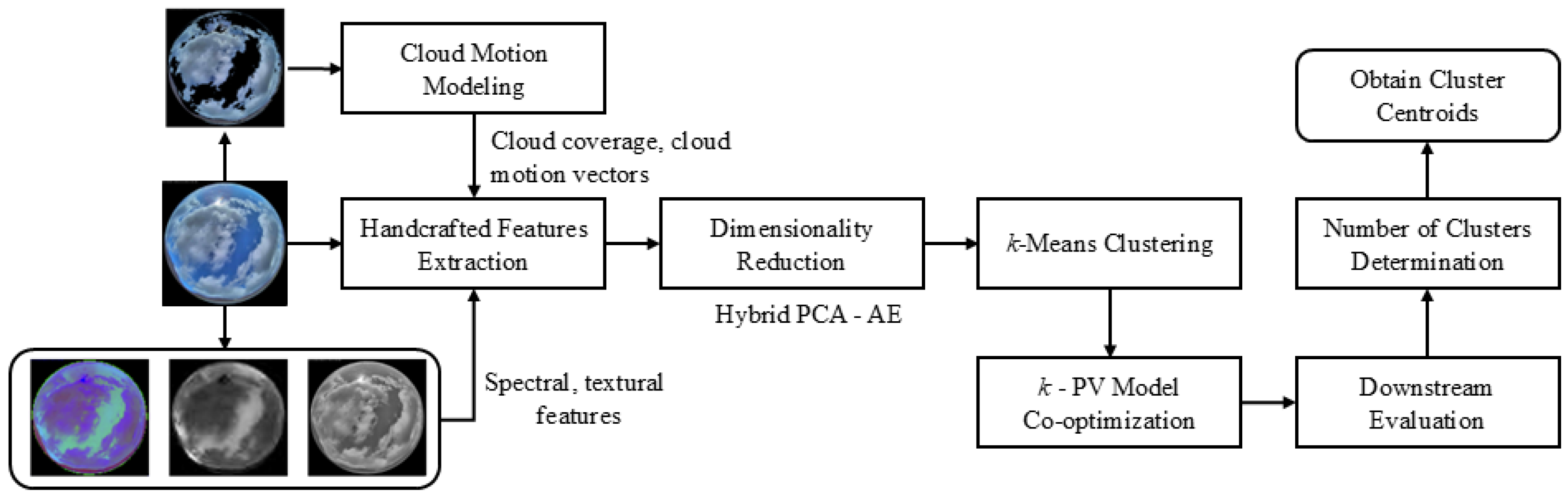
Figure 6.
Sky image examples per cluster: (1) Overcast; (2) Sunny; (3) Clear sky, sun near sunset; (4) Almost overcast; (5) Clear sky, sun near sunrise; (6) Sun low on the horizon, partial cloud cover; (7) Partial cloud cover, thin clouds; (8) Partial cloud cover, thick clouds.
Figure 6.
Sky image examples per cluster: (1) Overcast; (2) Sunny; (3) Clear sky, sun near sunset; (4) Almost overcast; (5) Clear sky, sun near sunrise; (6) Sun low on the horizon, partial cloud cover; (7) Partial cloud cover, thin clouds; (8) Partial cloud cover, thick clouds.
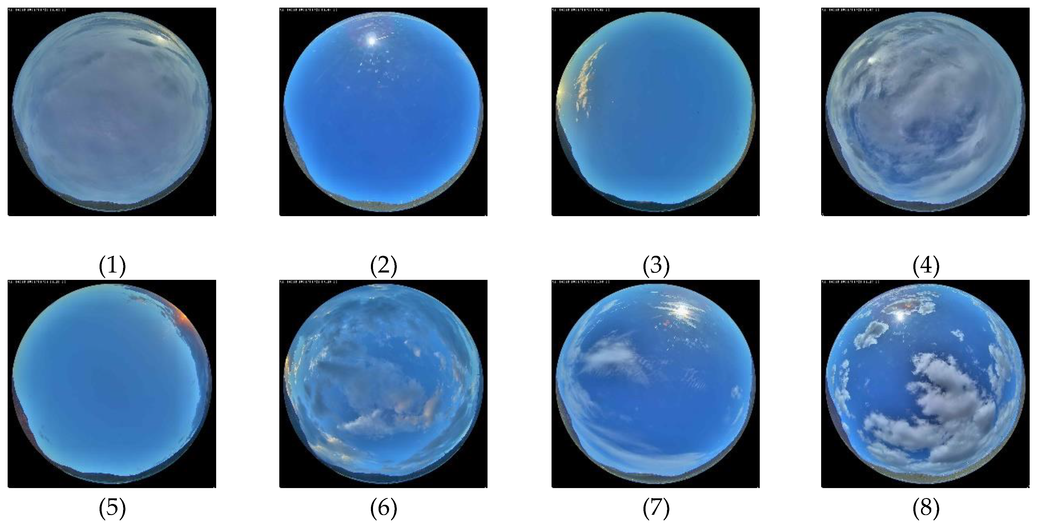
Figure 7.
Flow chart of the proposed sky image prediction process.
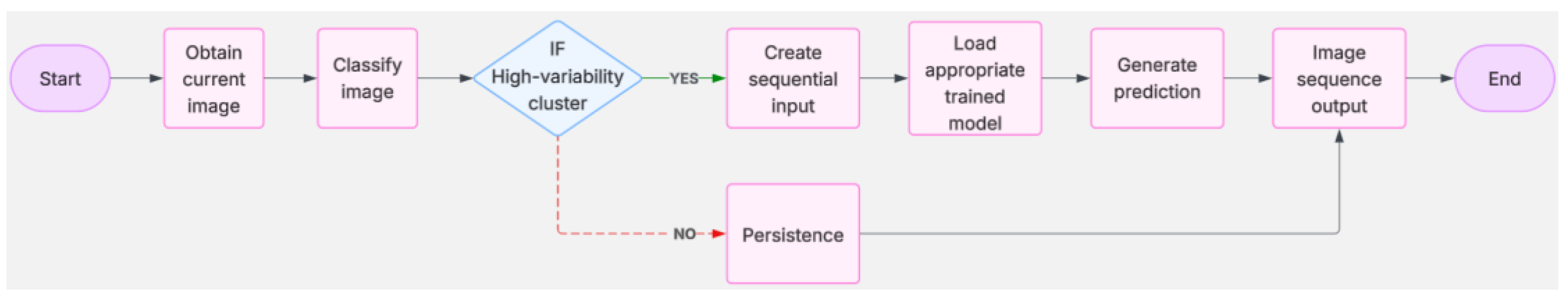
Figure 8.
Example of real and forecasted sequence for cluster 6.
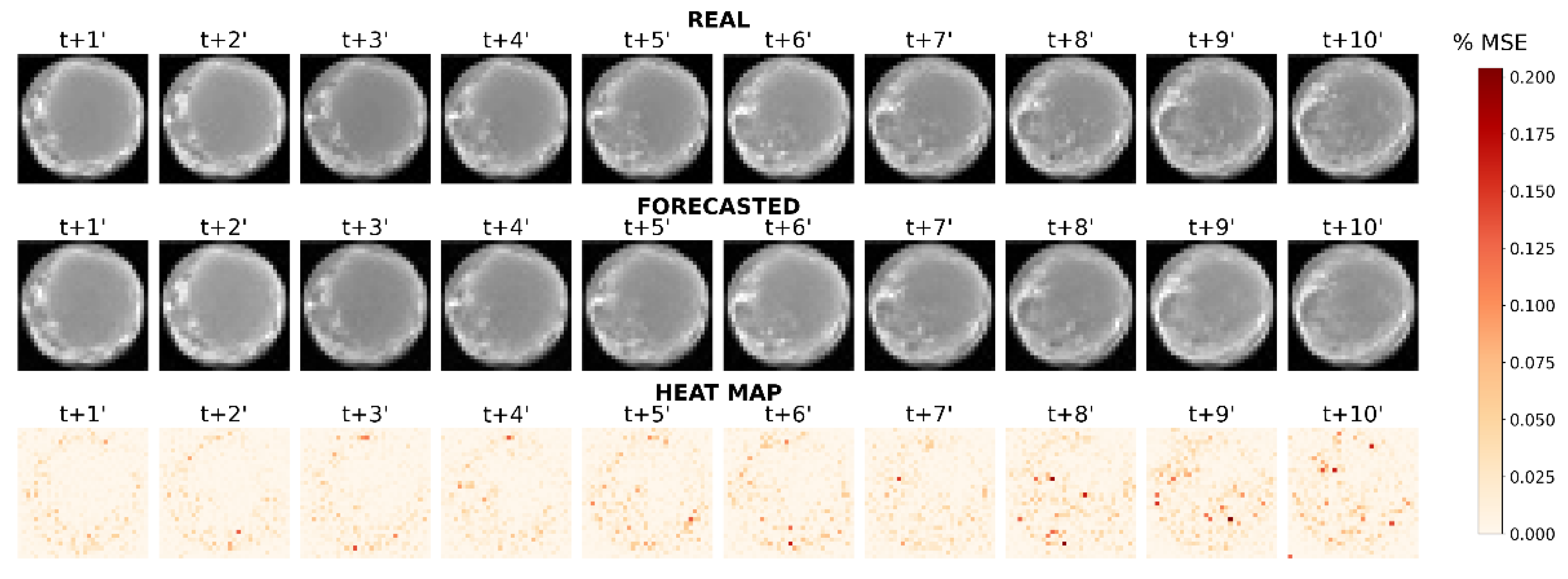
Figure 9.
Example of real and forecasted sequence for cluster 8.
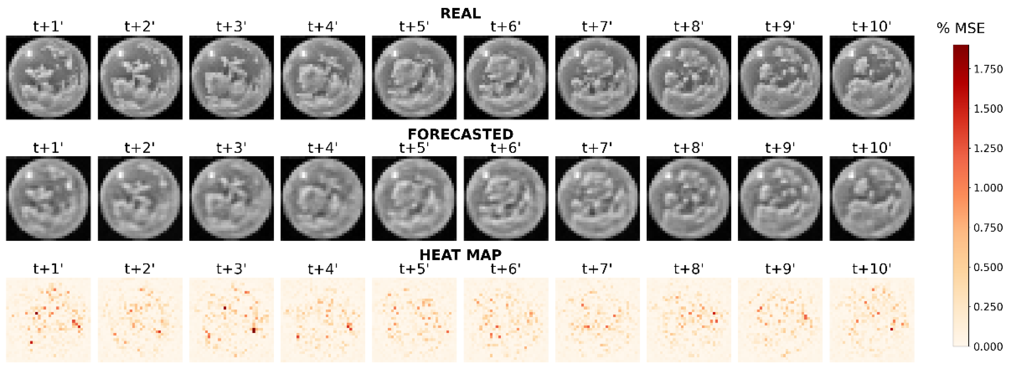

Table 1.
8-Cluster model sensitivity analysis.
| KS | NHL | Cluster 1 | Cluster 4 | Cluster 6 | Cluster 7 | Cluster 8 | |||||
|---|---|---|---|---|---|---|---|---|---|---|---|
| MSE | SSIM | MSE | SSIM | MSE | SSIM | MSE | SSIM | MSE | SSIM | ||
| 3 | 5 | 1.2971 | 59.08 | 0.157 | 67.24 | 1.0872 | 58.16 | 0.1182 | 78.78 | 0.2921 | 62,2 |
| 3 | 7 | 0.7376 | 64.82 | 0.1041 | 79.11 | 1.1235 | 60.71 | 0.0928 | 83.36 | 0.169 | 79.35 |
| 3 | 9 | 0.0408 | 89.29 | 0.0619 | 88.66 | 1.0422 | 48.07 | 0.0804 | 87.80 | 0.0981 | 89.41 |
| 3 | 11 | 0.8922 | 68.18 | 0.0635 | 88.06 | 1.26 | 57.12 | 0.0805 | 87.21 | 0.1247 | 86.6 |
| 5 | 5 | 1.0360 | 60.82 | 0.1328 | 72.44 | 1.2877 | 54.83 | 0.1298 | 80.63 | 0.2448 | 69.26 |
| 5 | 7 | 0.0450 | 88.03 | 0.0562 | 89.37 | 2.0304 | 36.64 | 2.0543 | 28.05 | 1.8057 | 27,12 |
| 5 | 9 | 0.0354 | 90.57 | 0.038 | 92.68 | 0.2552 | 89.59 | 1.9815 | 25.28 | 0.0773 | 91.31 |
| 5 | 11 | 0.0155 | 96.34 | 0.049 | 91.01 | 2.0244 | 55.5 | 0.0304 | 95.12 | 0.051 | 95.3 |
| 7 | 5 | 0.6987 | 65.78 | 0.117 | 76.09 | 4.1567 | 20.14 | 0.1181 | 80.28 | 1.1463 | 41.59 |
| 7 | 7 | 1.014 | 58.35 | 0.0536 | 89.91 | 2.3391 | 32.4 | 3.3495 | 19.46 | 2.1185 | 32.86 |
| 7 | 9 | 1.124 | 55.27 | 0.0455 | 92.14 | 0.0774 | 98.5 | 10.9458 | 13.64 | 5.5331 | 25.66 |
| 7 | 11 | 0.63 | 78.08 | 0.0408 | 92.46 | 0.2265 | 94.97 | 2.9834 | 32.5 | 1.5028 | 33.53 |
Table 2.
Models’ Assessment Metrics.
| Model | MSE (%) | SSIM (%) |
|---|---|---|
| Persistence | 0.197 | 76.1 |
| OF | 0.239 | 86.51 |
| 1-Cluster AE-like CNN | 0.14 | 80.18 |
| 3-Cluster AE-like CNN | 0.093 | 84.54 |
| 6-Cluster AE-like CNN | 0.057 | 93.78 |
| 8-Cluster AE-like CNN (proposed) | 0.053 | 94.59 |
Table 3.
Per-cluster results for the proposed 8-Cluster AE-like CNN model.
| Cluster | Model | Sequences | MSE (%) | SSIM (%) |
|---|---|---|---|---|
| 1 | AE-like CNN | 936 | 0.0155 | 96.34 |
| 2 | Persistence | 1963 | 0.029 | 96.13 |
| 3 | Persistence | 561 | 0.0858 | 92.27 |
| 4 | AE-like CNN | 1442 | 0.038 | 92.68 |
| 5 | Persistence | 794 | 0.1678 | 90.39 |
| 6 | AE-like CNN | 517 | 0.0774 | 98.5 |
| 7 | AE-like CNN | 885 | 0.0304 | 95.12 |
| 8 | AE-like CNN | 753 | 0.051 | 95.3 |
| Aggregate | 7851 | 0.053 | 94.59 |
Table 4.
8-Cluster model with and without per-cluster sensitivity analysis.
| Cluster | Model | MSE (%) | SSIM (%) | ||
|---|---|---|---|---|---|
| With | Without | With | Without | ||
| 1 | AE-like CNN | 0.0155 | 0.0775 | 96.34 | 81.73 |
| 2 | Persistence | 0.029 | 0.029 | 96.13 | 96.13 |
| 3 | Persistence | 0.0858 | 0.0858 | 92.27 | 92.27 |
| 4 | AE-like CNN | 0.038 | 0.1533 | 92.68 | 68.08 |
| 5 | Persistence | 0.1678 | 0.1678 | 90.39 | 90.39 |
| 6 | AE-like CNN | 0.0774 | 0.266 | 98.5 | 73.65 |
| 7 | AE-like CNN | 0.0304 | 0.113 | 95.12 | 78.97 |
| 8 | AE-like CNN | 0.051 | 0.286 | 95.3 | 62.12 |
| Aggregate | 0.053 | 0.139 | 94.59 | 83.73 | |
Table 5.
Dataset splits’ results.
| Model | MSE (%) | SSIM (%) | ||
|---|---|---|---|---|
| 70-15-15 | 50-25-25 | 70-15-15 | 50-25-25 | |
| 1-Cluster AE-like CNN | 0.14 | 0.17 | 80.18 | 80.1 |
| 3-Cluster AE-like CNN | 0.093 | 0.089 | 84.54 | 86.27 |
| 6-Cluster AE-like CNN | 0.057 | 0.085 | 93.78 | 86.36 |
| 8-Cluster AE-like CNN | 0.053 | 0.055 | 94.59 | 93.02 |
Disclaimer/Publisher’s Note: The statements, opinions and data contained in all publications are solely those of the individual author(s) and contributor(s) and not of MDPI and/or the editor(s). MDPI and/or the editor(s) disclaim responsibility for any injury to people or property resulting from any ideas, methods, instructions or products referred to in the content. |
© 2025 by the authors. Licensee MDPI, Basel, Switzerland. This article is an open access article distributed under the terms and conditions of the Creative Commons Attribution (CC BY) license (http://creativecommons.org/licenses/by/4.0/).
Copyright: This open access article is published under a Creative Commons CC BY 4.0 license, which permit the free download, distribution, and reuse, provided that the author and preprint are cited in any reuse.


