
Submitted:
29 September 2025
Posted:
30 September 2025
You are already at the latest version
Abstract
Conditioning is a very useful way of using correlated information to reduce the variability of an estimate. Inference based on a conditioned estimate, can be much more precise than on an unconditioned estimate. Here we give expansions in powers of $n^{-1/2}$} for the conditional density and distribution of a multivariate standard estimate based on a sample of size $n$. Standard estimates include most estimates of interest, including smooth functions of sample means and other empirical estimates. So they have potential application to a range of practical problems. We also show that a conditional estimate is not a standard estimate, so that Edgeworth-Cornish-Fisher expansions cannot be applied directly.
Keywords:
conditional distributions
; multivariate Edgeworth expansions
; Edgeworth coefficients
; standard estimates
MSC: Classification 62E20
1. Introduction and Summary
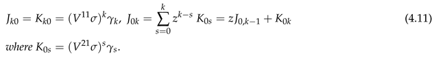
Suppose that is a standard estimate of an unknown parameter of a statistical model, based on a sample of size n. That is, is a consistent estimate, and for , its rth order cumulants have magnitude and can be expanded in powers of . This is a very large class of estimates, with potential application to a range of practical problems. For example, may be a smooth function of one or more sample means, or a smooth functional of one or more empirical distributions. A smooth function of a standard estimate is also a standard estimate: see [29]. [32] gave the multivariate Edgeworth expansions for the distribution and density of
in powers of about the multivariate normal in terms of the Edgeworth coefficients of (2.3). (For typos, see p25 of [29]. Also replace by on 4th to last line p1121 and in (23). To line 3 p1138, add .) [30] gave the Edgeworth coefficients explicitly for the Edgeworth expansions to . [15].
We now turn to conditioning. This is a very useful way of using correlated information to reduce the variability of estimates, and to make inference on unknown parameters more precise. This is the motivation for this paper. In Section 3 we take , and write and as , and of dimensions . Just as the distribution of allows inference on w, the conditional distribution of given , allows inference on for a given . The covariance of can be substantially less than that of . Only when and are uncorrelated, is there no advantage in conditioning.
Theorems 3.1 and 3.2 give our main results: explicit expansions to for the conditional density and distribution of given , that is, for the conditional density and distribution of given . In other words it gives the likely position of for any given . The main difficulty is integrating the density. Theorem 3.2 does this in terms of of (3.28), the integral of the multivariate Hermite polynomial, with respect to the conditional normal density. Note 3.1 gives in terms of derivatives of the multivariate normal distribution. Theorem 3.3 gives in terms of the partial moments of the conditional distribution. If , then Theorem 3.4 gives in terms of the unit normal distribution and density.
Section 4 specialises to the case . Examples are the condtional distribution and density of a bivariate sample mean, of entangled gamma random variables, and of a sample mean given the sample variance. Section 5 and Section 6 give conclusions, discussion, and suggestions for future research. Appendix A gives expansions for the conditional moments of It shows that given , is neither a standard estimate, nor a Type B estimate, so that Edgeworth-Cornish-Fisher expansions do not apply to it.
2. Multivariate Edgeworth Expansions
Suppose that is a standard estimate of with respect to n. (n is typically the sample size.) That is, as , where we use for expected value, and for and the rth order cumulants of can be expanded as
where ≈ indicates an asymptotic expansion, and the cumulant coefficients may depend on n but are bounded as . So the bar replaces each by k. For example and We reserve for this bar notation to avoid double subscripts.
the multivariate normal on , with density and distribution
V may depend on n, but we assume that is bounded away from 0.
for . These are Bell polynomials in the cumulant coefficients of (2.1), as defined and given in [30]. Their importance lies in their central role in the Edgeworth expansions of of (2.2).
(When and is a sample mean, the Edgeworth coefficients were given for all r in [31]. For typos, see p24–25 of [29].) Set Probability A is true. By [32], or [29], for non-lattice, the distribution and density of can be expanded as
is the multivariate Hermite polynomial. We use the tensor summation convention, repetition of in (2.6) implies their implicit summation over their range, . [30] gave explicitly for and for when .
where sums over all N permutations of giving distinct values. For example,
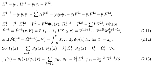 (So the repeated in (2.11) implies their repeated summatioin over .) are given explicitly in [30]. So (2.4) with the in [30] give the Edgeworth expansions for the distribution and density of of (2.2) to . and each have terms, but many are duplicates as is symmetric in . This is exploited by the notation of Section 4 of [30] to greatly reduce the number of terms in (2.6).
By (2.5), the density of relative to its asymptotic value is
and for measurable ,
If , then for r odd, so that
Examples 3 and 4 of [30] gave for
, and .
3. The Conditional Density and Distribution
For and partition and as and where are vectors of length . Partition as where are .
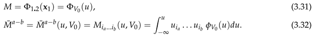
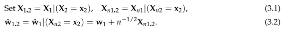 Now we come to the main purpose of this paper. Theorem 3.1 expands the conditional density of about the conditional density of . Its derivation is straightforward, the only novel feature being the use of Lemma 3.2 to find the reciprocal of a series, using Bell polynomials. Theorem 3.2 integrates the conditional density to obtain the expansion for the conditional distribution of about the conditional distribution of in terms of of (3.28) below, the integral of the Hermite polynomial of (2.8), with respect to the conditional normal density. Note 3.1 gives in terms of derivatives of the multivariate normal distribution. Theorem 3.3 gives in terms of the partial moments of the conditional normal distribution. For of (3.1), set
Lemma 3.1.
The elements of are
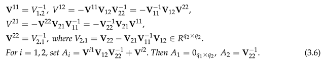
PROOF gives 8 equations relating and . Now solve for .
So for
Since in the sense that for , is less variable than , and is less variable than , unless and are uncorrelated, that is, is a matrix of zeros.
The conditional density of is
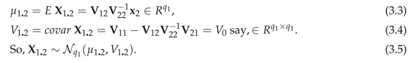
where is of (2.6) for , and is the density of of (3.1). By (4)–(6), Section 2.5 of [1], for of (3.4),
So the distribution of is
For of (3.3), of (3.4), and , set
Corollary 3.1.
Suppose that . Then for of (3.9),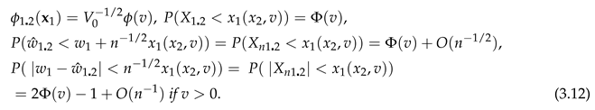
If , this gives an asymptotic conditional confidence limit for given . So if , by (2.14), for of (3.11), 2-sided limits are
So is given by replacing and in by
By (2.5) and (2.6), for , of (3.8) is given by
and implicit summation in (3.14) for is now over . So,
Ordinary Bell polynomials. For a sequence from R, the partial ordinary Bell polynomial , is defined by the identity
where for They are tabled on p309 of [7]. To obtain (3.7), we use
Lemma 3.2.

Take of (3.15). Set for . Then
PROOF
Now swap summations. □
Theorem 3.1.
Take of (2.6) and of (3.16) with
The conditional density of (3.7), relative to of (3.9), is
and for sequences and So,

PROOF This follows from (3.7) and Lemma 3.2. □
So of (3.20) and (3.21) give the conditional density to . We call (3.19) the relative conditional density. We now give our main result, an expansion for the conditional distribution of . As noted, Theorem 3.2 gives this in terms of of (3.28) below, an integral of the Hermite polynomial of (2.8), and Note 3.1 gives in terms of derivatives of the multivariate normal distribution. Theorem 3.3 gives in terms of the partial moments of the conditional distribution of (3.10). When , Theorem 3.4 gives in terms of and for
Theorem 3.2.
Take of Theorem 3.1. Set The conditional distribution of given , about of (3.10), has the expansion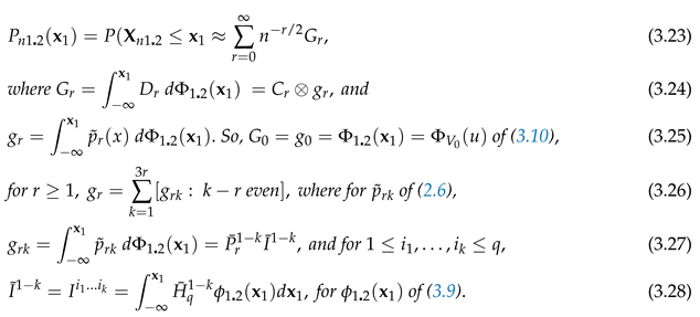
PROOF (3.26) holds by (2.6). (3.27) holds by (2.6). Now use (3.9). □
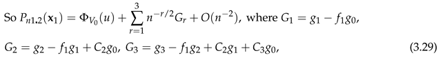 for of (3.17). is given by , is given by and is given by
for of (3.17). is given by , is given by and is given by
Note 3.1. Set By (3.9),
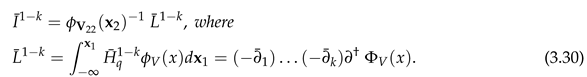 Comparing with the Hermite function of (2.7), we can call the partial Hermite function. When , see (4.1).
Comparing with the Hermite function of (2.7), we can call the partial Hermite function. When , see (4.1).By (3.25), in (3.23) is given by of (3.18) and of (3.26). Viewing as a polynomial in for u of (3.9), is linear in
for . So can be expanded in terms of the partial moments of
 This has only integrals, while (2.12) has q integrals.
This has only integrals, while (2.12) has q integrals.
Lemma 3.3.
For , , where
PROOF , where , and for of (3.6). □
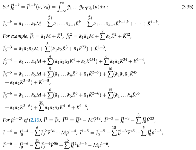
Our main result, Theorem 3.2, gave the conditional distribution expansion in terms of of (3.28). Note 4.1 gave these in terms of the derivatives of . We now give in terms of , the partial moments of the conditional distribution of (3.10). As in (2.10), for any , set summed over all, N say, permutations of giving distinct . For example, .
Theorem 3.3.
Take of (2.11), u of (3.10), M of (3.31), of (3.32), of (3.33), and
. Set
where sum over their range So ,
PROOF Since Substitute into the expressions for Now multiply by and integrate from to
This gives the needed for . The needed for can be written down similarly in terms of the partial moments using for We now show that if , we only need the partial moments of at v of (3.22), and that these are easily written in terms of and a polynomial in v of (3.22).
The case So
Theorem 3.4.
For , is given by Theorem 3.3 with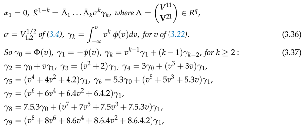 where dot denotes multiplication. Also, .
where dot denotes multiplication. Also, .
PROOF For v of (3.22), by (3.9), (3.37) follows from integration by parts. By (3.34), where
That follows from (3.25). □
By (3.23), for of (3.18) and v of (3.22), the conditional distribution of is
as in (3.29), and is given by (3.26) in terms of the integrated Hermite polynomial, of (3.28) given by Theorems 3.3, 3.4.
4. The Case
Theorem 3.2 gave the conditional Edgeworth expansion in terms of of (3.28). Theorem 3.3 gave needed for of (3.27) and of (3.23), in terms of the partial moments of (3.32). When , Theorem 3.4 gave in terms of and its partial moments for v of (3.22). But now so that or 2. So for of (2.9), we switch notation to
 for of (3.30). Similarly, write (2.1) as
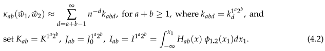 Also, we switch from to
Theorem 4.1.
The conditional density of of (3.1), is given by Theorem 3.1 where is given by (3.14) in terms of
PROOF This follows from Theorem 3.1. □
Theorem 4.2 gives a laborious expression for the conditional distribution.
However Theorem 4.3 gives a huge simplification.
Theorem 4.2.
The conditional distribution of of (3.1), is given by Theorem 3.2 with of Theorem 3.4 as follows. For even, of (3.27) is given by
where of (4.2) is given for , as follows in terms of .
Also are with and of (3.33) reversed, before setting and by (3.13). For example, by (4.9), for of Theorem 3.4,
PROOF This follows from Theorems 3.3 and 3.4. □
This gives the needed for for the conditional distribution of (3.23)–(3.25) to . The needed for can be written down similarly. We now give a much simpler method for obtaining of (3.27), and so by (3.26), and needed for (3.23) by (3.24). Theorem 4.3 gives and in terms of of (4.2). Theorem 4.4 gives in terms of of (4.11), a function of of Theorem 3.4.
Theorem 4.3.
For v of (3.22), of (4.2) is given by
For and even, of (3.27) is given by
So by (3.26), for of (3.25) is given by
PROOF By (4.8),
By (3.9), where and So,
This proves (4.12). So,
(4.13) follows. (4.14) now follows from (3.14). □
Note 4.1. is just of (4.3) with replaced by for .
So for is given in terms of of Section 3, by
 This gives and of (3.26) for , and so the conditional distribution of (3.23), to , in terms of of (4.2) and the coefficients .
This gives and of (3.26) for , and so the conditional distribution of (3.23), to , in terms of of (4.2) and the coefficients .
Theorem 4.4.
The needed for of (4.14) and (3.24) are given in terms of of (3.22), and of (4.11), by
PROOF For follow from Theorem 3.2. By the proof of Theorem 3.3, can be read off [30] and the univariate Hermite polynomials given in terms of by expanding
To summarise, the conditional density of of (3.1), is given by Theorem 4.1, and the conditional distribution is given by (3.23), (3.27) in terms of of (4.14) and of Theorem 4.4.
Example 4.1.
 The relative conditional density is given to by (3.19) in terms of of (2.6), of (4.3), of (3.14) for , and of (4.4) for .
The conditional distribution is given by (3.38) with of (4.14), starting
of Theorem 4.4, and of (4.19). As noted this is a far simpler result than using Theorem 4.2.
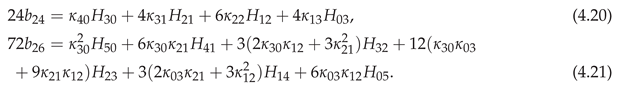
for of (4.20), (4.21) and above.
The relative conditional density is given to by (3.19) in terms of of (2.6), of (4.3), of (3.14) for , and of (4.4) for .
The conditional distribution is given by (3.38) with of (4.14), starting
of Theorem 4.4, and of (4.19). As noted this is a far simpler result than using Theorem 4.2.
for of (4.20), (4.21) and above.
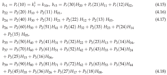
Conditioning when is the mean of a sample with cumulants . The non-zero were given in Example 6 of [30]. So for and for other are given by (4.15)–(4.18) starting
The relative conditional density is given to by (3.19) in terms of of (2.6), of (4.3), of (3.14) for , and of (4.4) for .
Example 4.2.
We now build on
the entangled gamma
model of Example 7 of [30], which gave the needed. Let be independent gamma random variables with means . For , set , and let be the mean of a random sample of size n distributed as . So, and where are independent gamma random variables with means . The rth order cumulants of are and otherwise . Now suppose that ,
the entangled exponential
model. So , and have correlation ,
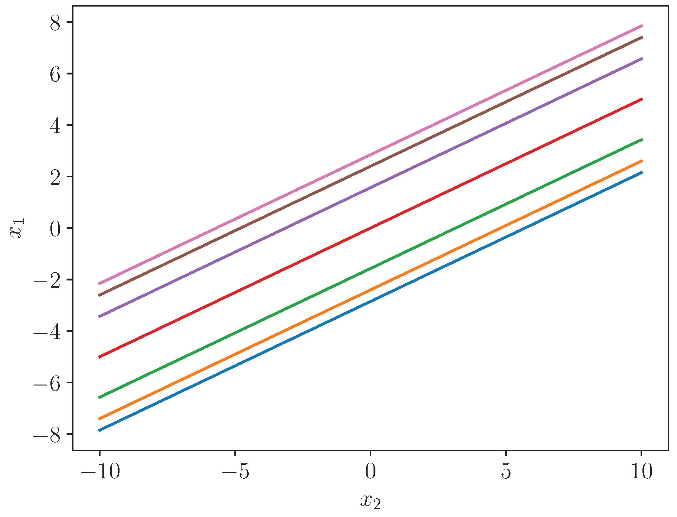
for of (3.11), that is, . Figure 4.1 plots the conditional asymptotic quantiles of , that is, , for . To , given n and , this figure is equivalent to a figure of versus . That is, Figure 4.1 shows to , the likely value of for a given value of In fact by (3.12), lies between the outer limits with probability .98+. So although labelled as versus , the figure can be viewed as showing the likely value of for a given value of
We now give of (3.17), of (3.19), and of (4.4), and for , the coefficients of the expansion for the conditional distribution of (3.23).
By Note 4.1, of Example 7 of [30], symmetry, and (4.14),
Let us work through 2 numerical examples to get the conditional distribution to . We build on Example 7 of [30]. By Theorem 4.1, if then ,
We worked to 8 significant figures, but display less. If , then
So to the relative conditional density of (3.19) for is
so that for and 16 we can only include two terms, and for , only three terms. We now give the 1st 3 , needed by (3.23) for the conditional distribution to . By (3.36),
. By (3.3), .
For example for to
so that divergence begins with the 4th term.
So to the relative conditional density of (3.19) for is
so that we can only include three terms. Finally, we now give the 1st three , needed by (3.23) for the conditional distribution to .
For example for to
so that divergence begins with the 3rd term.
Example 4.3.
Conditioning when the distribution of is symmetric about w. Then for r odd, . By (3.19), the conditional density is
for of Example 1 of [30], of (4.4), and
By (3.38), the conditional distribution of is
for of (4.16) and (4.17).
Example 4.4.
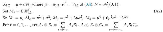
Discussions of pivotal statistics advocate using the distribution of a sample mean, given the sample variance. So Let be the usual unbiased estimates of the mean and variance from a univariate random sample of size n from a distribution with rth cumulant . So By the last 2 equations of Section 12.15 and (12.35)–(12.38) of [26], the cumulant coefficients needed for of (2.3) for , – the coefficients needed for the conditional density to , in terms of , are
(3.19) gives in terms of and , that is, in terms of and of (3.14) in terms of . In this example, many of these are 0. The non-zero are in order needed,
For is now given by (2.13), , and Section 2 of [30]. By (2.4) and (3.19), this gives the conditional density to . And (4.14) gives needed for the conditional distribution to .
5. Conclusions
[30] gave the density and distribution of to , for any standard estimate, in terms of functions of the cumulant coefficients of (2.1), called the Edgeworth coefficients, .
Most estimates of interest are standard estimates, including smooth functions of sample moments, like the sample skewness, kurtosis, correlation, and any multivariate function of k-statistics. (These are unbiased estimates of cumulants and their products, the most common example being that for a variance.) Unbiased estimates are not needed for Edgeworth expansions, although this does simplify the Edgeworth coefficients, as seen in Examples 4.1, 4.2, 4.4. However unbiased estimates are not available for most parameters or functions of them, such as the ratio of two means or variances, except for special cases of exponential families. [29] gave the cumulant coefficients for smooth functions of standard estimates.
As noted, conditioning is a very useful and basic way to use correlated information to reduce the variability of an estimate. Section 3 gave the conditional density and distribution of given to where is any partition of . The expansion (3.19) gave the conditional density of any multivariate standard estimate. Our main result, an explicit expansion for the conditional distribution (3.23) to , is given in terms of the leading of (3.28). These are given explicitly by Theorems 3.3 and 3.4.
When Theorem 4.1 simplified the conditional density expansion, and Theorem 4.3 gave a huge simplification, and the coefficients of the conditional distribution expansion in terms of of Theorem 4.4.
6. Discussion
A good approximation for the distribution of an estimate, is vital for accurate inference. It enables one to explore the distribution’s dependence on underlying parameters. Our analytic method avoids the need for simulation or jack-knife or bootstrap methods while providing greater accuracy than any of them. [13] used the Edgeworth expansion to show that the bootstrap gives accuracy to . [12] said that “2nd order correctness usually cannot be bettered”. But this is not true using our analytic method. Simulation, while popular, can at best shine a light on behaviour, only when there is a small number of parameters, and only for limited values of their range.
Estimates based on a sample of independent, but not identically distributed random vectors, are also generally standard estimates. For example, for a univariate sample mean where has rth cumulant , then where is the average rth cumulant. For some examples, see [22,23] and [32] , 2020). The last is for a function of a weighted mean of complex random matrices. For conditions for the validity of multivariate Edgeworth expansions, see [24] and its references, and Appendix C of [30].
While the use of Edgeworth-Cornish-Fisher expansions is widespread, few papers address how to deal with their divergence for small sample sizes. [8] and [11] avoided this question as it did not arise in their examples. In contrast we confronted this in Example 4.2, the examples of Withers (1984), and in Example 7 of [30].
We now turn to conditioning. Conditioning on makes inference on more precise by reducing the covariance of the estimate. The covariance of can be substantially less than that of . [3] pp34-36 argue that an ideal choice would be when the distribution of does not depend on . But this is generally not possible except for some exponential families. An example when it is true, is when and are location and scale parameters: on p54 they essentially suggest choosing . This is our motivation for Example 4.4. For some examples, see [2]. Their (7.5) gave a form for the 3rd order expansion for the conditional density of a sample mean to , but did not attempt to integrate it.
Tilting (also known as small sample asympotics, or saddlepoint expansioins), was first used in statistics by [9]. He gave an approximation to the density of a sample mean, good for the whole line, not just in the region where the Central Limit Theorem approximation holds. A conditional distribution by tilting, was first given by [25] up to , for a bivariate sample mean. Compare [2]. For some other results on conditional distributions, see [5,10,14,21], Hansen (1994), [20], Chapter 4 of [6], and [17].
Future directions. The results here give the first step for constructing confidence intervals and confidence regions of higher order accuracy. See [15] and [28]. What is needed next, is an application of [29] to obtain the cumulant coefficients of or those of . This should be straightforward.
2. When , our expansion for the conditional distribution of of (3.1), can be inverted using the Lagrange Inversion Theorem, to give expansions for its percentiles. This should be straightforward. (The quantile expansions of [8] and Withers (1984) do not apply as Appendix A shows that conditional estimates of standard estimates are not standard estimates.)
3. Here we have only considered expansions about the normal. However expansions about other distributions can greatly reduce the number of terms by matching the leading bias coefficient. The framework for this is [32], building on [15]. For expansions about a matching gamma, see [33,36].
4. The results here can be extended to tilted (saddlepoint) expansions by applying the results of [32]. The tilted version of the multivariate distribution and density of a standard estimate are given by Corollaries 3, 4 there, and that of the conditional distribution and density follow from these. For the entangled gamma of Example 4.2, this requires solving a cubic. See also [16].
5. A possible alternative approach to finding the conditional distribution, is to use conditional cumulants, when these can be found. Section 6.2 of [18] uses conditional cumulants to give the conditional density of a sample mean to . Section 5.6 of [19] gave formulas for the 1st 4 cumulants conditional on only when and are uncorrelated. He says that this assumption can be removed, but gives no details how. That is unlikely to give an alternative to our approach, for as well as giving expansions for the first 3 conditional cumulants, Appendix A shows that the conditional estimate is not a standard estimate.
6. Lastly we discuss numerical computation. We have used [27] for our calculations. Its input is and , - not and . There is a function sub2(sb1,sb2) which takes as argument the two subscripts of mu, and returns the value. If global variables mu20, mu02, mu11 are symbolic variables (defined using sympy) then it returns the answer in terms of those, but if they are numeric then it returns a numeric answer. There is another function called biHermite(n, m, y1, y2) which takes the 2 subscripts of H. If y1 and y2 are symbolic, then it returns a symbolic answer, but if they are numeric it returns a numeric answer. A numerical example is given by Example 4.2, that is, for the case and or .
Similar software for numerical calculations for Theorems 4.1, 4.3 and 4.4 would be invaluable, as would software for applying the Lagrange Inversion Theorem. (We mention R-4.4.1 for Windows: dmvnorm for the density function of the multivariate normal, mvtnorm for the multivariate normal, qmvnorm for quantiles, and rmvnorm to generate multivariate normal variables.) On bivariate Hermite polynomials, see cran.r-project.org/web/packages/calculus/vignettes/hermite.html
Appendix A Conditional Moments
Here we give expansions for the conditional moments of of (3.1), in terms of the conditional normal moments of , of (3.1). And we show that
is neither a standard estimate of , nor a Type B estimate, as defined below.
Consider the case . By (3.5),
 Non-central moments.
Non-central moments.
Theorem A1.
Take of Theorem 3.1. Set For the sth conditional moment of of (3.1) about of (3.10), has the expansion
PROOF This follows from Theorem 3.1 □
So by (A3), the sth conditional moment of is
of (A5) and (A6). For example,
So of (A1) is not a standard estimate, as by (A3), the expansion for its mean is a power series in , not . Is it a Type B estimate? These are defined as for a standard estimate, but with cumulant expansions being series in , not . We shall see. Take . By Theorem 4.2, for of (2.3), of (A4) is given by
For example,
Finding the
The needed are given in Appendix B of [30] in terms of
For example,
Let us write in terms of of (Appendix A2), as
To get a general formula for , set
where if is odd. is just of Appendix B of [30] with V replaced by
Central moments. Set and .
For of (A3), set
Is the conditional estimate a Type B estimate? This requires its rth cumulant to have magnitude for . This is true for and 2 but not for , as has magnitude , since .
References
- Anderson, T. W. (1958) An introduction to multivariate analysis. John Wiley, New York.
- Barndoff-Nielsen, O.E. and Cox, D.R. (1989). Asymptotic techniques for use in statistics. Chapman and Hall, London.
- Barndoff-Nielsen, O.E. and Cox, D.R. (1994). Inference and asymptotics. Chapman and Hall, London.
- Bhattacharya, R.N. and Rao, Ranga R. (2010). Normal approximation and asymptotic expansions, SIAM edition.
- Booth, J., Hall, P. and Wood, A. (1992) Bootstrap estimation of conditional distributions. Annals Statistics, 20 (3), 1594–1610. [CrossRef]
- Butler, R.W. (2007) Saddlepoint approximations with applications, pp. 107–144, Cambridge University Press. [CrossRef]
- Comtet, L. Advanced Combinatorics; Reidel: Dordrecht, The Netherlands, 1974.
- Cornish, E.A. and Fisher, R. A. (1937) Moments and cumulants in the specification of distributions. Rev. de l’Inst. Int. de Statist. 5, 307–322. Reproduced in the collected papers of R.A. Fisher, 4. [CrossRef]
- Daniels, H.E. (1954) Saddlepoint approximations in statistics. Ann. Math. Statist. 25, 631–650.
- DiCiccio, T.J., Martin, M.A. and Young, G.A. (1993) Analytical approximations to conditional distribution functions. Biometrika, 80 4, 781–790.
- Fisher, R. A. and Cornish, E.A. (1960) The percentile points of distributions having known cumulants. Technometrics, 2, 209–225. [CrossRef]
- Hall, P. (1988) Rejoinder: Theoretical Comparison of Bootstrap Confidence Intervals Annals Statistics, 16 (3),9 81–985.
- Hall, P. (1992) The bootstrap and Edgeworth expansion. Springer, New York.
- Hansen, B.E. (1994) Autoregressive conditional density estimation. International Economic Review, 35 (3), 705–730. [CrossRef]
- Hill, G.W. and Davis, A.W. (1968) Generalised asymptotic expansions of Cornish-Fisher type. Ann. Math. Statist., 39, 1264–1273. [CrossRef]
- Jing, B. and Robinson, J. (1994) Saddlepoint approximations for marginal and conditional probabilities of transformed variables. Ann. Statist., 22, 1115–1132. [CrossRef]
- Kluppelberg, C. and Seifert, M.I. (2020) Explicit results on conditional distributions of generalized exponential mixtures. Journal Applied Prob., 57 3, 760–774. [CrossRef]
- McCullagh, P., (1984) Tensor notation and cumulants of polynomials. Biometrika 71 (3), 461–476. McCullagh (1984).
- McCullagh, P., (1987) Tensor methods in statistics. Chapman and Hall, London.
- Moreira, M.J. (2003) A conditional likelihood ratio test for structural models. Econometrica, 71 (4), 1027–1048. [CrossRef]
- Pfanzagl, P. (1979). Conditional distributions as derivatives. Annals Probability, 7 (6), 1046–1050.
- Skovgaard, I.M. (1981a) Edgeworth expansions of the distributions of maximum likelihood estimators in the general (non i.i.d.) case. Scand. J. Statist., 8, 227-236.
- Skovgaard, I. M. (1981b) Transformation of an Edgeworth expansion by a sequence of smooth functions. Scand. J. Statist., 8, 207-217.
- Skovgaard, I. M. (1986) On multivariate Edgeworth expansions. Int. Statist. Rev., 54, 169–186.
- Skovgaard, I.M. (1987) Saddlepoint expansions for conditional distributions, Journal of Applied Prob., 24 (4), 875–887. [CrossRef]
- Stuart, A. and Ord, K. (1991). Kendall’s advanced theory of statistics, 2. 5th edition. Griffin , London.
- Teal, P. (2024) A code to calculate bivariate Hermite polynomials.https://github.com/paultnz/bihermite/blob/main/hermite8.py.
- Withers, C.S. (1989) Accurate confidence intervals when nuisance parameters are present. Comm. Statist. - Theory and Methods, 18, 4229–4259. [CrossRef]
- Withers, C.S. (2024) 5th-Order multivariate Edgeworth expansions for parametric estimates. Mathematics, 12,905, Advances in Applied Prob. and Statist. Inference. https://www.mdpi.com/2227-7390/12/6/905/pdf.
- Withers, C.S. (2025) Edgeworth coefficients for standard multivariate estimates. New Perspectives in Mathematical Statistics, 2nd Edition. Axioms 2025.
- Withers, C.S. and Nadarajah, S.N. (2009) Charlier and Edgeworth expansions via Bell polynomials. Probability and Mathematical Statistics, 29, 271–280.
- Withers, C.S. and Nadarajah, S. (2010) Tilted Edgeworth expansions for asymptotically normal vectors. Annals of the Institute of Statistical Mathematics, 62 (6), 1113–1142. [CrossRef]
- Withers, C.S. and Nadarajah, S. (2011) Generalized Cornish-Fisher expansions. Bull. Brazilian Math. Soc., New Series, 42 (2), 213–242. DOI:�¿¡10.1007/s00574-011-0012-9 Some typos: p217 line 7. Replace stem by step. p220. Replace the first two words “That is,” by “Suppose now that”. p220. After “replace” in line 6, insert “Yn by -Yn,”. p 226. Replace lines 5–7, “Suppose that ... This is”, as follows. “Suppose that for ν in Np and |ν|=∑j=1pνj,lν=na(|ν|)λν satisfies . (7.3) This is”. p226. Replace κr on LHS of 4th displayed equation by kr. p226. Replace kr on RHS of 6th displayed equation by Kr. p227. Replace r in (7.5) and the following equation by |ν|. p227 Replace “variance” in (7.6) by “covariance”.
- Withers, C.S. and Nadarajah, S. (2012) Nonparametric estimates of low bias. REVSTAT Statistical Journal, 10 (2), 229–283.
- Withers, C.S. and Nadarajah, S. (2014a) Bias reduction: The delta method versus the jackknife and the bootstrap. Pakistan Journal of Statist., 30 (1), 143–151.
- Withers, C.S. and Nadarajah, S. (2014b) Expansions about the gamma for the distribution and quantiles of a standard estimate. Methodology and Computing in Applied Prob., 16 (3), 693-713. DOI 10.1007/s11009-013-9328-9 For typos, see p25–26 of Withers (2024). [CrossRef]
- Withers, C.S. and Nadarajah, S. (2023) Bias reduction for standard and extreme estimates. Commun. Statistics - Simulation and Comp., 52 (4), 1264–1277. [CrossRef]
Figure 4.1.
of (3.11) for - courtesy of Dr Paul Teal:
Disclaimer/Publisher’s Note: The statements, opinions and data contained in all publications are solely those of the individual author(s) and contributor(s) and not of MDPI and/or the editor(s). MDPI and/or the editor(s) disclaim responsibility for any injury to people or property resulting from any ideas, methods, instructions or products referred to in the content. |
© 2025 by the authors. Licensee MDPI, Basel, Switzerland. This article is an open access article distributed under the terms and conditions of the Creative Commons Attribution (CC BY) license (http://creativecommons.org/licenses/by/4.0/).
Copyright: This open access article is published under a Creative Commons CC BY 4.0 license, which permit the free download, distribution, and reuse, provided that the author and preprint are cited in any reuse.


