Submitted:
28 September 2025
Posted:
29 September 2025
You are already at the latest version
Abstract
The problem of the article is to increase the efficiency of biometric authentication of personnel of critical infrastructure facilities. It is shown that one of the main directions of increasing efficiency is to improve the procedure for selecting facial contours in the test image, the result of which is the determination of a rectangular area that does not provide accurate selection of facial contours and interference during video recording. To overcome these limitations, it is advisable to use neural network semantic segmentation tools that allow you to accurately select facial contours, the eye area, as well as areas with overlaps or background elements. At the same time, known solutions in the field of semantic segmentation show that most of them do not provide the possibility of effective functioning in the conditions of critical infrastructure facilities. In order to overcome these shortcomings, the article has developed a method for determining the architectural parameters of a neural network model of semantic segmentation of a facial image during biometric authentication at critical infrastructure facilities. The method allows taking into account the specifics of the expected conditions for the use of semantic segmentation tools and provides an opportunity to reduce the number of experimental studies related to the determination of the architectural parameters of the neural network model by up to 10 times. The results of experimental studies confirm that the model developed as a result of the implementation of the proposed method provides a 1.1-1.2-fold increase in the accuracy of semantic segmentation of a face image and allows reducing the influence of background diversity and interference, which improves the quality of input data, which is subsequently used for face recognition.
Keywords:
cybersecurity
; information security
; critical infrastructure facility
; biometric authentication
; semantic segmentation
; neural network model
; facial image
1. Introduction
In the context of increasing challenges in the field of national security, automated access control systems for critical infrastructure facilities play a special role [1,2,3]. One of the key components of such systems is biometric authentication tools that provide identification of a person based on a facial image. To ensure high accuracy and reliability of identification, a preliminary stage is necessary - semantic image segmentation, which allows you to highlight the face area among other fragments of the scene. At the same time, in real conditions, the task of semantic segmentation is significantly complicated due to the need to take into account a number of various factors, in particular, partial or complete overlap of the face with foreign objects (personal protective equipment, glasses, hair, etc.), variability of shooting angles, changes in lighting, as well as various parameters of video or photo fixation (resolution, number of color channels, etc.). All this necessitates the use of tools that can adapt to complex and unstable environmental conditions. In most known biometric authentication systems, these tools are based on neural network image processing technologies, which have already demonstrated high efficiency in computer vision tasks. Their ability to detect complex spatial relationships, generalize features at different levels of abstraction, and adapt to new data makes them a promising tool for implementing accurate and reliable face recognition in biometric authentication systems.
As the results of scientific and practical work in the field of biometric authentication show, in most modern solutions, the identification of a person by an image of a face is carried out on the basis of its selection using a rectangular frame (bounding box), which is set by detection algorithms, in particular, based on models such as MTCNN, RetinaFace, BlazeFace, YOLO, etc. [4,5,6,7,8,9]. However, this approach has a number of limitations: first, it does not take into account the natural shape of the face, which reduces the accuracy of subsequent processing stages, such as normalization, feature extraction and their comparison; second, rectangular localization does not allow to correctly separate interference - for example, hair, masks, gloves, overlaps or background falling within the frame [10,11]. As a result, this approach can lead to a deterioration in the recognition accuracy and an increase in the sensitivity of the system to external factors or spoofing attacks. In this context, there is growing interest in the use of neural network methods of semantic segmentation, which provide pixel-wise division of the image into logical regions. This allows to more accurately highlight the contours of the face and interference zones, improving the quality of background masking or exclusion of irrelevant areas [12,13]. Unlike bounding box approaches, pixel segmentation forms an adaptive mask that preserves the shape of the object and increases the reliability of subsequent identification [14]. The advantages of semantic segmentation are especially noticeable in conditions of variable lighting, non-standard angles or partial overlaps, which often occur in practical scenarios of biometric authentication systems [7]. Therefore, at the next stage of the analysis, attention is focused on scientific and practical works devoted to the development of solutions in the field of semantic segmentation, which can find their application in biometric authentication systems based on facial images.
One of the promising approaches to semantic image segmentation, which allows to work effectively with a limited amount of annotated data, is proposed in [15]. Here, a generative model was developed that performs pixel segmentation based on the generative-adversarial architecture StyleGAN2 with an additional branch of label synthesis. It is declared that the advantage of the approach is the support of semi-supervised learning: the model is trained on a large number of unannotated images supplemented with a relatively small amount of labeled data. Segmentation at the testing stage is performed by projecting the image into the latent space of the joint distribution of “image-label” and generating the corresponding mask. The solution showed high accuracy in medical segmentation tasks, as well as in segmentation of parts of the face. However, when using this approach in biometric authentication tasks, a number of potential limitations should be taken into account. In particular, generative models may exhibit instability of results when working with data with a high level of variability in facial details. This may affect the predictability and repeatability of segmentation results, which is critically important in security systems. In addition, additional computational costs associated with optimization in the latent space at the testing stage may complicate the integration of such a solution into real software and hardware complexes. In [16], an approach to the use of convolutional neural networks for multi-class segmentation of facial images captured using a thermal imaging camera is proposed. It is noted that the architecture of the neural network model is developed using the “image-to-image translation” approach and adapted to facial image segmentation for medical purposes, which involves monitoring possible signs of infectious diseases using temperature analysis of facial areas. The article [17] is devoted to solving the problem of increasing the accuracy of semantic segmentation and localization of key points of the face by using neural network models for training which used exclusively synthetic data, which were created by integrating a parameterized 3D face model with various textures and background images. It is noted that the use of synthetic data provides the possibility of building neural network solutions in cases where the collection or annotation of real data is complicated. It should be noted that the use of synthetic data in the field of biometric authentication requires additional research related to the insufficient stability of the results obtained when implementing the generative approach. In the article [18], a method of semantic image segmentation is proposed that does not require labeled data. The approach is based on the use of the StyleGAN2 generative model, in the latent space of which clustering is performed, which allows to highlight semantically significant areas. Based on these clusters, a synthetic dataset is created, which is used to train the segmentation model. Additionally, the CLIP model is used, which allows detecting object classes based on text queries, even if the corresponding labels are absent in open datasets. The results obtained demonstrate the ability of the model to generate masks that are well consistent with human ideas about semantic classes, while the segmentation model trained on synthetic data effectively generalizes to real images. However, the application of the proposed method in biometric authentication systems is limited by the complexity of controlling the accuracy of the selection of critically important areas of the face, the dependence on the quality of clustering in the latent space, and the limited stability of the models when generating rare or borderline classes. In the article [19], an approach to improving the accuracy of face recognition based on deep features obtained from RGB-D images is proposed. The authors focus on the problem of limited availability of large 3D facial datasets, which leads to insufficiently effective training of neural network models. To solve it, two models are presented: DepthNet - a network for estimating the depth map taking into account semantic segmentation, and Mask-Guided RGB-D Network - an architecture that combines RGB, depth and segmentation mask processing branches with a spatial attention module. A feature of DepthNet is the use of a segmentation mask to improve face localization and build a reliable depth map based only on RGB images. The generated depth maps are used to enrich the 2D dataset and form a large RGB-D training set. Using the obtained experimental data, it is shown that the proposed architecture demonstrates high resistance to variations in head position and, from the point of view of segmentation accuracy, surpasses known basic methods on several 3D datasets. At the same time, insufficient attention is paid in the work to the issues of adapting the neural network architecture to application conditions that do not concern the spatial parameters of the test face image. In the article [20], the prospects for the application of neural network models of semantic segmentation of a face image in the task of detecting falsified faces and determining areas that have been manipulated are considered. Although in the context of the biometric authentication task, the results of the work have certain prospects, however, in this article the issue of developing effective neural network tools for semantic segmentation is not considered fully enough. A similar conclusion can be drawn regarding the article [21], which proposes the DML-CSR method, which is based on decorrelated multitask learning with a cyclic self-regulation mechanism and, according to the authors, will significantly reduce the typical errors of modern face segmentation models - spatial inconsistency and blurred boundaries between classes.
For the completeness of the analysis, a number of works were considered, devoted to the most modern approaches to semantic segmentation of various types of images. Based on the results of [22], it was determined that modern neural network models designed for semantic segmentation of images can be divided into two clusters. The first cluster includes models whose architecture is based on the traditional scheme of convolutional neural networks: a fully convolutional network [23], U-Net [24], U-Net++ [25], as well as models whose architectural foundations are used in DeepLabV3+ implementations [26,27,28]. This also includes simplified versions of segmentation models integrated into the MediaPipe framework, focused mainly on real time and mobile devices. Most of the known research within this cluster focuses on the optimization of the encoder component, while improving the decoder capabilities for high-dimensional feature reconstruction and accurate recovery of fine spatial details are often neglected [22,29,30]. This architectural imbalance limits the effectiveness of these models in segmenting facial images under variable illumination, partial occlusions, and limited resolution. The second cluster includes neural network models whose architecture includes attention mechanisms [31,32,33]. Such solutions demonstrate high potential in terms of improving segmentation accuracy, but are accompanied by a significant increase in computational complexity. It should be noted that most modern neural network solutions - in particular, in the models implemented in DeepLabV3+ and in the MediaPipe (Selfie Segmentation) framework - do not provide a formalized adaptive mechanism for selecting architectural and training parameters, which is critically important under the conditions of increased requirements for the accuracy and stability of the model in the tasks of semantic face segmentation. In addition, a separate cluster of quite promising, but little-studied architectures is considered, in particular the BiSeNet V1 model [34], which combines two specialized branches - semantic and detailed — with the Guided Aggregation mechanism. Such an architecture demonstrates high performance with acceptable accuracy, however, due to the complexity of the feature fusion mechanisms and the limitations of controlled control of decoding accuracy, its application in high-responsibility biometric authentication systems is not yet widespread. Thus, the results of the analysis of modern scientific and practical works in the field of semantic facial segmentation indicate that most existing solutions are focused on the development or borrowing of universal neural network architectures that demonstrate high efficiency on common test sets, but do not take into account the specifics of application in biometric authentication systems on critical infrastructure facilities, in particular the requirements for ensuring an acceptable level of accuracy, time and computational resource intensity of segmentation, as well as for correct execution of segmentation in conditions of partial interference on the face. In addition, despite significant achievements, the task of operational development of neural network tools for semantic segmentation, adapted to the expected conditions of application, remains insufficiently formalized and researched. This indicates the relevance of developing a method that will ensure the operational construction of neural network tools for semantic segmentation of facial images, adapted to the conditions of use in biometric authentication systems for personnel of critical infrastructure facilities, which determines the purpose of this study.
2. Materials and Methods
2.1. Peculiarity of Segmentation Mask Formation in the Context of Biometric Authentication
According to the results of [10,35], in biometric authentication systems, semantic segmentation of facial images should be performed taking into account the informativeness of its individual zones. In the simplest case, only two areas are distinguished - the background and the face within their natural contours, without detailing the internal components. In more complex cases, the eyes, eyebrows, nose, mouth and hair are also subject to segmentation, since their selection helps to increase the accuracy of positioning the face and iris during further biometric processing. Hair associated with a hairstyle can also be selected in cases where its contours are used to normalize the position of the head. Elements that cover or distort the face (glasses, masks, jewelry, etc.) should be considered as background and not included in the segmentation mask. Thus, depending on the applied rules of zone selection, the number of segmentation classes in the model can vary - from two (face/background) to several, detailing the structure of the face. It is worth noting that the resulting masks are subsequently synchronized with the original images, based on which an image is formed that is used to detect spoofing attacks and recognize faces.
2.2. Development of a Semantic Facial Image Segmentation Model
Using as a prototype the author's developments in the field of application of neural networks for image segmentation [35,36], it was determined that in the basic case the model of semantic segmentation of a facial image during biometric authentication at critical infrastructure facilities (M_{SS}) can be described using expressions of the form:
where is the input face image to be segmented, is the probability map of pixel classes, is the segmentation function (), is the set of real numbers, and are the height and width of the image, is the number of color channels in the image, is the number of segmentation classes, is the intensity of the с-th color channel of the pixel with coordinates and is the probability that the pixel with coordinates belongs to the k-th class.
Note that in common image representation formats, the brightness values of each color channel are stored as integers. For example, when using the RGB format, it is quite common to record the brightness of each pixel using an 8-bit number. This means that , where – is a set of integers, and the brightness of each of the color channels of an arbitrary pixel is an integer from 0 to 255. However, in practice, the standard procedure for preparing an image before feeding it to the input of a neural network model involves scaling the brightness of each of the color channels to the range , by dividing the initial brightness value of each pixel by a number corresponding to the maximum possible brightness value, for example, by 255 for 8-bit images. Therefore, in expression (1) .
Considering that, according to the results of [25,35,37], for semantic segmentation it is advisable to use a neural network model, the architecture of which involves the use of an encoder and a decoder, expression (1) can be modified as follows:
where is the function that describes the result of applying the neural network encoder, and is the function that describes the result of applying the neural network decoder.
Using the results of [37,38,39], it was determined that in the basic case, the functionality of a neural network encoder and a neural network decoder can be described using expressions of the form (5) and (6), respectively. Note that according to the results of [27,30,40,41,42], it is advisable to use such types of neural network models as VGG, ResNet, MobileNet, EfficientNet, HRNet as the basis of the encoder and decoder. It is believed that the most tested types of encoder and decoder are based on VGG models and are used in U-Net-like neural network models of semantic segmentation with possible omissions of subsampling layers and a variable number of convolution layers..
where is the feature tensor of the encoded image, is the size of the convolution/subsampling maps at the output of the encoder, and is the number of convolution/subsampling maps at the output of the encoder (the depth of the feature space).
A detailed description of the procedure for the functioning of the encoder (5) can be carried out using expressions (7, 8), and to detail the functioning of the decoder (6) - expressions (9, 10).
where – two-dimensional feature matrix at the output of the c-th convolution map in the l-th convolutional layer (); – number of convolution layers in the encoder; – two-dimensional feature matrix at the output of the s-th subsampling map; – weights corresponding to the c-th convolution map in the first convolutional layer; – subsampling operation; – activation function in the first convolutional layer of the encoder.
where – two-dimensional feature matrix corresponding to the c-th convolution map in the n-th convolutional layer of the decoder (); – number of convolution layers in the decoder; – concatenation (skip-connection) of weight coefficients from the corresponding encoder level.
In this case, according to [43,44], the term upsampling describes a procedure that is implemented by increasing the spatial resolution of the feature tensor, which is performed in the neural network decoder in order to step-by-step restore the original image size after downsampling, i.e. compression due to the passage of the input image through the encoder. The upsampling procedure can be described as follows:
where upsampling result; height and width of the input feature tensor ;
height and width of the upsampling kernel ; upsampling scaling factor; function for determining the nearest smallest integer; upsampling kernel value at position .
The values of depend on the interpolation method used and are determined using expressions of the form:
where Kronecker delta function; fixed parameter (); function that corresponds to the definition of as a result of training the neural network model.
Expression (12) is used when applying the nearest neighbor interpolation method, expression (13) - for two-dimensional linear interpolation; expressions (14, 15) - for bicubic interpolation, and expression (16) - when determining the upsampling kernel as a result of training a neural network model.
Integration of expressions (5-16), taking into account the features of the functioning of a decoder based on a convolutional neural network, allows us to write the resulting expression for calculating the pixel class probability map in the following form:
where – weight coefficients of the last convolutional layer of the neural network decoder; – a function describing the implementation of the upsampling procedure in the neural network decoder.
In the most common case of using a Softmax-type activation function in the neurons of the output layer of the decoder, the probability that a pixel with coordinates belongs to the k-th class can be calculated as follows:
where – the decoder output signal (logit), representing a non-normalized estimate of whether a pixel with coordinates belongs to the k-th class.
We also note that the specificity of the task of recognizing the face of a representative of the personnel of a critical infrastructure facility indicates the need to obtain the result of semantic segmentation not only in the form of a probability map of pixel classes, but also in the form of a segmented image of the face, which displays its natural boundaries, eye boundaries and interference boundaries. Taking into account [35,38], the definition of such a segmented image can be implemented by assigning each pixel of this image to the class with the highest probability. That is:
where is the class to which the image pixel with coordinates belongs; is the probability of assigning the pixel with coordinates to the k-th class; is the segmented image.
Taking into account the results of [42,43,44], the analysis of the developed mathematical support (1-20) of the neural network model of semantic segmentation of the face image of a representative of the personnel of a critical infrastructure facility, built on the basis of a U-Net-like architecture, indicates that the list of design parameters of this model, which ensure the possibility of its adaptation to the expected conditions of application, includes: the number of convolution layers and the number of convolution maps, the size and step of the convolution kernel in each of the layers for the encoder and decoder; the number and localization of the encoder subsampling layers; the number and localization of the upsampling layers; the kernel size, scale factor and interpolation method for each of the upsampling layers; number of skip-connections, localization of the input in the encoder and insertion into the decoder of each of the skip-connections; number of aggregation levels of skip-connection features; skip-connection aggregation variant. Note that in the case of using alternative architectures (ResNet, VGG, MobileNet, EfficientNet, HRNet) as the basis of a neural network model of semantic segmentation, the list of design parameters is additionally expanded due to the type of encoder, parameters of multi-scale context modules, attention blocks, strategies for combining multi-level features and methods of semantic post-processing. Thus, for an encoder and decoder that provide for the use of Residual blocks characteristic of the ResNet neural network, the functioning of which is described by expressions (21, 22), the list of design parameters should include: number of stages, number of blocks in each of the stages, convolution parameters for each block and parameters of the projecting convolution.
where – j-th Residual-block at the first stage; – input tensor of the first stage; – the number of stages; – sequence of convolutions/upsampling in the Residual block; - set of parameters of convolution/upsampling layers; – set of convolution/upsampling parameters to reduce the dimension to the dimension .
In addition, based on [45,46,47], the list of design parameters includes parameters that characterize the learning procedure: the type of optimizer (for example, Adam, SGD), the size of the mini-package (batch size), the learning rate (learning rate), the strategy for changing the learning rate (learning rate scheduling), the conditions for stopping training (early stopping, number of epochs), regularization methods (dropout, batch normalization, etc.), as well as the type of loss function. Using the data [31,35,48], it was determined that the following types of loss functions are usually used in neural network models of semantic segmentation: Categorical Cross-Entropy, Binary Cross-Entropy, Dice Loss, Jaccard Loss, Focal Loss, Tversky Loss. Note that the Categorical Cross-Entropy loss function is defined by the expression (23), Binary Cross-Entropy – (24), Dice Loss – (25, 26), Jaccard Loss – (27, 28), Focal Loss – (29), Tversky Loss – (30, 31).
where is the number of pixels in the image; is the number of classes; is the resulting segmentation mask; is the true segmentation mask; are the sets of pixels that fall into the categories true positive, false positive and false negative; is the predicted probability of pixel belonging to class ; is the true label; is the coefficient used to avoid division by 0; is the weighting factor for class k; is the focusing parameters; are the weights for pixels belonging to the sets FP and FN, respectively.
According to [48], , , are taken, and the value of is set to be inversely proportional to the fraction of pixels of class in the training data set. Given that in the process of building neural network tools for semantic segmentation, specific indicators are used that reflect the features of the training sample, the learning process and the specifics of the results of semantic segmentation, the mathematical support of the semantic segmentation model includes the training sample imbalance coefficient (), the variance of the gradients of the loss function (), he coefficient of deviation of the position of the boundaries of the selected object from the true boundaries (), the coefficient of the relative size of the object mask (), the average value of the standard deviation of the brightness and the range of the average brightness values of the images in the training sample. The calculation of these coefficients is provided using expressions (32-40). In this case, the training sample imbalance coefficient is calculated as follows:
where is the number of pixels of class k in the whole sample.
Note that . In case when , the sample is considered balanced, and the case corresponds to a significant imbalance in the training sample.
The variance of the loss function gradients is calculated as the relative standard deviation of the loss function gradient , calculated over several consecutive epochs:
where is the standard deviation and the average value of during training epochs; is the gradient of loss function .
The coefficient of deviation of the position of the boundaries of the selected object from the true boundaries is calculated using the expressions:
where is the set of pixels of the contour of the predicted mask for the k-th object; is the set of pixels of the contour of the true mask for the k-th object; is the total number of pixels in the predicted contours of all objects (normalization factor); is the minimum Euclidean distance from pixel to the nearest pixel of the true contour .
The coefficient of the relative size of the object mask is calculated as:
where is the number of objects in the sample; is the number of pixels in the mask of the j-th object in the i-th image; is the total number of pixels in the i-th image; is the number of objects in the i-th image.
The average value of the standard deviation of the brightness and the range of the average values of the brightness RV of the images in the HSV format in the training sample are calculated according to expressions (37-40). In this case, the brightness (channel V) is expressed as an integer in the range from 0 to 255.
where is the number of examples (images) in the training sample; is the standard deviation of the brightness values in the n-th image; is the array of brightness channel values in the nth image; is the average brightness value of the nth image; is the width and height of the image.
In conclusion, expressions (1-40) form the basis for describing the mathematical apparatus of the semantic segmentation model, which, due to the use of the encoder-decoder architecture of a neural network with variable design parameters that are subject to adaptation depending on the application conditions, provides the possibility of developing an effective method for determining the architectural parameters of the neural network model of semantic segmentation of a face image during biometric authentication at critical infrastructure facilities.
2.3. Formation of Rules for Determining Architectural Parameters of a Neural Network Model of Semantic Segmentation
Since, according to [35,36,39], it is advisable to implement the definition of the mechanism for forming the set of admissible architectures and training parameters outside the semantic segmentation model, the next step of the research is associated with the formation of a set of rules (), that regulate the relevant aspects of the development of neural network tools.
R1. Rule for forming the set of admissible basic architectures
The set of basic architectures is formed taking into account computational constraints, allowable segmentation time, image characteristics, class imbalance, variability of conditions and accuracy requirements. The set of basic architectures is formed by sequentially analyzing the key conditions of the semantic image segmentation problem:
- In the case of limited segmentation time and computational resources (allowable segmentation time - 100 ms, the amount of available memory for storing model parameters is less than 30 MB) - MobileNet, EfficientNet(B0-B1).
- For images in RGB format up to 256×256 - VGG (U-Net, U-Net++, or Attention U-Net++), MobileNet.
- If the number of segmentation classes does not exceed 3 - MobileNet, VGG (U-Net), and otherwise - VGG (U-Net++ or Attention U-Net++), ResNet, HRNet.
- If it is necessary to segment small objects (the area of the object occupies less than 0.1 of the area of the input image) and with a high imbalance of object examples (the imbalance coefficient is less than 0.2) to be segmented in the training sample - VGG (U-Net++ or Attention U-Net++), HRNet.
- With high variability of lighting and angle of video recording of the face image after preprocessing (the ranges of lighting and angle of video recording exceed the threshold values defined in [111], in the first approximation 0.5) - VGG (U-Net++ or Attention U-Net++), ResNet, EfficientNet, HRNet.
- If it is necessary to achieve high accuracy (IoU > 0.85) - VGG (U-Net++ or Attention U-Net++), ResNet, HRNet.
- If the total number of training examples , and the allowable number of training epochs - priority is given to models that achieve fast convergence on small samples (MobileNet, EfficientNet, ResNet-18, VGG (U-Net)).
- If - priority is given to models that are characterized by high initial convergence and stability of loss dynamics (ResNet-34, EfficientNet, VGG (U-Net++)).
- In cases where none of the basic architectures satisfies all the requirements, the use of MobileNet is envisaged as a compromise model that provides the optimal balance between processing speed and segmentation quality.
Using the results of [22,38,42], it is determined that it is appropriate, depending on the number of weight coefficients (), to distinguish three complexity classes of neural network architectures: low complexity, for which , medium complexity - and high complexity - . In particular, low complexity models include MobileNet and EfficientNet-B0, medium complexity models include ResNet-18, ResNet-34, U-Net (VGG) and Attention U-Net, and high complexity models include ResNet-101, HRNet, U-Net++ and Attention U-Net++.
R2. Training data augmentation rule.
The rule defines the mechanism for augmenting training data, which is carried out to increase the model's generalization ability. In the basic version, augmentation mechanisms of the type:
- Random Crop, which randomly limits the image to 90% of its original size. This allows the model to better focus on local areas of the face;
- Gaussian Noise with a standard deviation of σ < 0.01, which simulates noise typical of camera sensors and increases the resistance to interference in the input image.
In addition, in the case of detecting significant variability in brightness characteristics in the training sample, Random Brightness/Contrast augmentation is applied: stochastic change in brightness and contrast with an amplitude within ±15%. The decision on the presence of significant variation is made if the average value of the standard deviation or the range , which are calculated according to expressions (37, 38).
R3. Loss function selection rule
The selection is implemented from the list of loss functions defined by expressions (23-31), taking into account the number of segmentation classes , the training sample imbalance coefficient , the deviation coefficient of the position of the boundaries of the selected object from the true boundaries and the coefficient of the relative size of the object mask , which are calculated according to expressions (32, 34-36).
- At . If Binary Cross-Entropy is used, if and - Focal Loss, and otherwise Dice Loss.
- At . If and - Jaccard Loss, and if - Dice Loss. If - Tversky Loss.
- At . If Categorical Cross-Entropy is used, if абo - Tversky Loss, and in other cases Dice Loss.
- With insufficient information or conflicting requirements - Dice Loss.
R4. Optimizer selection rule.
The rule defines an algorithm for optimizing the values of the neural network weight coefficients used during training to ensure stable convergence of the loss function, maintain stable dynamics of parameter updates throughout the training process, and achieve high segmentation quality under constraints on the training sample size and model complexity. Also, during training, the dynamics of the loss function on the validation sample is analyzed to confirm the effectiveness of the selected algorithm or make a decision on its correction. In this regard, rule R4 covers two levels of decision-making: the initial selection of the optimization algorithm (R4.1) and its adaptation during training (R4.2).
R4.1. Initial choice of optimization algorithm
- For models of medium and high complexity, in particular ResNet, HRNet, U-Net++, Attention U-Net, trained on limited samples () it is advisable to use the Adam optimizer, since it provides adaptive scaling of gradients and promotes stable convergence even in noisy or non-uniform gradient fields.
- For the same models of medium and high complexity, at the SGD optimizer with momentum (momentum=0.9) is used. This approach ensures stable convergence of the loss function and, provided there is a sufficient amount of data, allows achieving higher segmentation accuracy on validation data compared to adaptive methods.
- For models based on MobileNet and EfficientNet-B0 and at AdamW is used as a compromise solution between convergence speed and control over regularization.
R4.2. Optimization algorithm adaptation
- If during the training process a high dispersion of the gradients of the loss function is observed or instability of the dynamics of the loss function is observed, then the transition to the Adam optimizer is carried out. The dispersion of the gradients is considered high if the value >0,3 calculated according to expression (33) for at least 5 consecutive training epochs is considered unstable if its total decrease in 5 consecutive epochs is less than 1% or the amplitude of oscillations exceeds 20% of the average value in this interval.
R5. The rule for determining the learning rate parameters
The rule determines the learning rate parameters of a neural network model, which includes the selection of the initial value of the rate and the strategy for changing it during the learning process. This ensures stable convergence of the loss function, stable optimization dynamics throughout the entire learning period. Since the initial value of the rate is determined taking into account the complexity of the architecture, and the selection of the rate change strategy is implemented taking into account the size of the training sample, the permissible number of learning epochs and the features of the loss function convergence, the rule R5 covers three levels of decision-making: determining the initial value of the learning rate (R5.1), the initial selection of the strategy for changing the learning rate (R5.2) and adapting the strategy parameters to intermediate learning indicators (R5.3).
R5.1. Determining the initial value of the learning rate
The choice of the initial value of the learning rate is carried out from the standpoint of ensuring the stability of the learning process, which, according to [14,16,27], largely depends on the complexity of the neural network model, which in turn mainly depends on the number of weight coefficients (). Models of low complexity are characterized by limited depth and a small number of weight coefficients, therefore, the gradients of the loss function calculated at each iteration usually have a smaller norm, i.e. a relatively smaller absolute size of the change in weights. This reduces the risk of destabilization during parameter updates even with an increased learning rate. In other words, small models demonstrate less sensitivity to gradient fluctuations, and therefore can be effectively trained with a larger update step, which provides faster convergence in the initial phases of training. For such models, learning rate = 0.001. Models of medium complexity are characterized by a larger number of layers and weight coefficients, which leads to the accumulation of gradient errors in deeper layers. In such networks, the gradient norm (for example, in the L2 sense) can change from layer to layer - decrease (gradient decay effect) or increase (gradient explosion effect). Under these conditions, an increased learning rate value can lead to unstable oscillations in the optimization process, therefore, they require some reduction. Therefore, for models of medium complexity, learning rate = 0.0007. Models of high complexity are characterized by a large depth and a complex structure of connections (including residual blocks, attention mechanisms, etc.), which increases the probability of nonlinear growth of gradient norms in different parts of the network. This makes them especially sensitive to a large update step, since an excessive learning rate value can cause unstable weight updates, divergent behavior, or an explosion of activation values. Accordingly, for a high-complexity model, learning rate = 0.0005. The difference between the recommended learning rate values for medium- and high-complexity models is empirically based and is primarily focused on cases of using adaptive optimizers (Adam or AdamW). Thus,
- For neural network models based on MobileNet or EfficientNet-B0, which are low-complexity models, learning rate = 0.001.
- For neural network models based on ResNet-18, ResNet-34, U-Net (VGG) and Attention U-Net, which are medium-complexity models, learning rate = 0.0007.
- For neural network models based on ResNet-101, HRNet and models such as, U-Net++, Attention U-Net++, which are high-complexity models, learning rate = 0.0005.
R5.2. Choosing a learning rate change strategy
The choice of a learning rate change strategy is implemented from the standpoint of providing adaptive control of the learning rate, which allows for the effective use of available computational resources while maintaining the stability of the loss function optimization. The strategy is selected taking into account the permissible number of learning epochs () nd the total number of training examples ().
- If , then the Cosine Annealing strategy is used, which involves a gradual decrease in the learning rate along a cosine-like trajectory, which is the most acceptable strategy in conditions of limited training time, since it allows you to quickly pass the coarse optimization phase and gradually move to accurate local minimization.
- If , then the Step Decay strategy is used with a 10-fold decrease in the learning rate every 10 epochs, which avoids overtraining on a limited training sample.
- In other cases, the ReduceLROnPlateau strategy is used.
R5.3. Adaptation of the learning rate change strategy
- In the case of using the Cosine Annealing strategy, if after training during the first third of the specified number of training epochs () the loss function decrease is less than 0.5% over 5 epochs, the parameter of the strategy (the full length of the cosine phase) is reduced by 20%, which accelerates the learning rate decrease.
- In the case of using the Step Decay strategy, if after the first learning rate decrease (i.e. after 10 epochs) the loss function value increases or remains practically unchanged (decrease <1%) over the next 5 epochs, then the interval between learning rate decreases is reduced to 5 epochs.
- In the case of using the ReduceLROnPlateau strategy, if the loss function value on the validation sample does not decrease by more than 0.001 over 5 consecutive epochs, then the current learning rate value is reduced by 2 times.
At the same time, R5.3 takes into account the limits of changes in the parameters of the specified learning strategies, for the determination of which it is possible to use the results of [15,35].
Note that in rule R5 the type of input images and the architecture of the model are not directly taken into account, since these characteristics have already been used in the rule for selecting the basic architecture.
R6. Batch size selection rule.
The batch size selection is implemented taking into account the available computational resources (available amount of video memory of the graphics processor in bytes) (), the architectural complexity of the neural network model, the size of the input image and the dispersion of gradients, which allows for efficient use of hardware capabilities and to ensure the optimal ratio of speed and stability of convergence of the loss function. Accordingly, the R6 rule covers two levels of decision-making: selection of the batch size at the beginning of training (R6.1) and adaptation of the batch size to the training process (R6.2).
R6.1. Choosing the initial batch size
For neural network models based on ResNet-18, ResNet-34, U-Net (VGG) and Attention U-Net, which are medium complexity models with an image size of 256×256 pixels:
- If , then batch size = 4.
- If , then batch size = 8.
- If , then batch size = 16.
- If , then batch size = 32.
For neural network models based on MobileNet or EfficientNet-B0, which are low complexity models, the batch size increases twice, and for neural network models based on ResNet-101, HRNet and models such as, U-Net++, Attention U-Net++ , which belong to high complexity models, the batch size is reduced by half.
Also, the batch size is adjusted depending on the image size. For an image of size 512×512, the batch size is reduced by 4 times, for a size of 384×384, it is reduced by 2 times, and for a size of 128×128, it is increased by 2 times.
R6.2. Batch size adaptation
If during the learning process, during 5 consecutive learning epochs, the value of the variance of the gradients of the loss function () alculated using expression (33) exceeds 0.2, but is less than 0.3, i.e. when , provided that there is sufficient computing resources, the batch size increases by 2 times.
R7. Regularization mechanism selection rule
Adaptation of the regularization mechanism to the conditions of the segmentation problem is implemented to ensure a balance between the learning rate, the stability of the convergence of the loss function and the risk of overtraining. The type and parameters of the regularization mechanism are selected taking into account the number of training examples and the complexity of the model architecture, in particular the number of weight coefficients:
- In the case when the training sample size , is used to prevent overtraining, as well as L2-regularization with .
- For compact models based on the MobileNet or EfficientNet-B0 architectures, Dropout can negatively affect the convergence and efficiency of training. In this case, Dropout is not used, and to ensure uniform convergence dynamics and training rate, L2-regularization with .
- To reduce the risk of overfitting and stabilize weight coefficients when training models with more than parameters, such as ResNet (in configurations from ResNet-34 and higher), HRNet, Attention U-Net, U-Net++, Attention U-Net, Dropout with probability 0.3 is used, as well as L2-regularization with .
Note that the use of only Dropout and L2 regularization is explained by their proven effectiveness in applying neural networks for semantic image segmentation under conditions of limited computing resources..
R8. Rule for determining the number of training epochs
The number of training epochs () s determined from the standpoint of avoiding overtraining, ensuring the possibility of achieving the required segmentation accuracy taking into account the limited duration of training. This takes into account the convergence dynamics of the loss function, the maximum permissible number of training epochs, the volume and balance of the training sample.
R8.1. Determining the minimum number of training epochs
- If or the average number of examples of each class is less than 500, or (calculated according to (32)), then the minimum number of training epochs is 20. In other cases, the minimum number of training epochs is 30.
- If , then .
R8.2. Determining the conditions for stopping and continuing training
Training is stopped if, after the minimum number of training epochs, the loss function on the validation sample does not improve by more than 0.02 over the last 5 consecutive epochs, or a predetermined segmentation accuracy is achieved. Otherwise, provided that , training continues.
2.4. Development of a Method for Determining the Architectural Parameters of a Neural Network Model for Semantic Segmentation of Facial Images During Biometric Authentication at Critical Infrastructure Facilities
Using the method of semantic image segmentation described in [35] as a prototype, based on the proposed semantic segmentation model (1–40) and the formed set of rules for determining architectural parameters, the implementation of the proposed method for determining architectural parameters of a neural network model of semantic segmentation of a face image during biometric authentication at critical infrastructure facilities is divided into six stages. At the same time, taking into account the need to adapt to variable application conditions and the results of [39,42], the method is based on the principle of phased adaptation of the architecture, including the training parameters - first by initializing the maximum permissible values for a certain type of neural network model, and then through gradual modification of the model parameters taking into account the achieved accuracy, level of resource consumption and stability of the training process.
Stage 1. Determination of the conditions for developing a neural network model. The input of the stage is a tuple of , parameters describing the conditions of the biometric authentication task, regulatory requirements for the biometric authentication system, characteristics of the available training data set, a description of the developed semantic segmentation model and a set of rules , is formed, which regulate the development of neural network tools.
Step 1.1. Formalization of application conditions. Based on expert evaluation of the tuple of , and parameters, a tuple of , parameters is determined, which characterize: the size of the input image and the number of color channels (), the number of segmentation classes (); total number of training examples (), number of training examples for each segmentation element (), maximum available memory size for storing model parameters (), acceptable size for storing model parameters (), allowable term of the semantic segmentation process (), type and minimum allowable value of the segmentation accuracy indicator (), allowable number of training epochs (), as well as the training sample imbalance coefficient (), the coefficient of deviation of the position of the boundaries of the selected object from the true boundaries (), the coefficient of the relative size of the object mask (), he average value of the standard deviation of the brightness and the range of the average brightness values of the images in the training sample, which are calculated using expressions (32, 34, 36-38) respectively.
Step 1.2. Determination of available architectures. Based on expert evaluation, a set of available basic neural network architectures () is determined. By default, the specified set includes architectures based on VGG (U-Net, U-Net++, Attention U-Net++) and architectures such as ResNet, MobileNet, EfficientNet, HRNet. Based on expert evaluation, taking into account the results obtained during the development of the semantic segmentation model, the design parameters of each architecture included in and the range of values of these design parameters, which is determined by the set of minimum () and maximum values () are determined. Expert evaluation procedures are planned to be implemented based on the methods used in [10,47].
The output of the stage is a tuple of parameter values that characterize: restrictions related to segmentation tools, a set of available basic architectures, a set of design parameters of each of the basic architectures - . Note that the description of the developed semantic segmentation model and the formed set of rules received as input to the first stage are subsequently used in the execution of stages 2-6.
Stage 2. Selection of an architectural solution. The input to the stage is the tuple , determined as a result of the implementation of stage 1.
Step 2.1. Selection of admissible architectures. The selection is implemented based on the rule R1 taking into account the set of available architectures, computational constraints, image characteristics, class imbalance, variability of conditions and accuracy requirements defined in step 1.
Step 2.2. Selection of the base architecture. This step implements the selection of the architecture that will be used as the base. In the case when the implementation of the previous step leads to the selection of several architectures, then the architecture whose software and hardware implementation is less complex is selected as the base (A_{NB}). Also, in accordance with the defined type, from the standpoint of achieving maximum segmentation accuracy, a set of architectural parameters () is determined.
The output of step 2 is determined by the expression - .
Step 3. Determination of encoder parameters. The input of the stage is , , , – the correspondence between the value of the permissible and the value of the achieved accuracy indicator, which is determined as a result of the execution of stage 6. When performing stage 3 immediately after stage 2, it is assumed that .
Step 3.1. Initialization of encoder parameters. The step is performed in the case . he values of the encoder design parameters (5, 7, 8, 21, 22) are set equal to the values of the corresponding elements from the set для , тoбтo , where – is the number of the design parameter.
Step 3.2. Modification of encoder parameters. The step is performed in the case . In this case, the depth of the encoder (number of convolutional layers/number of stacks) changes according to expressions (41, 42).
where – number of the design parameter corresponding to the encoder depth.
Other encoder parameters are modified from the position of maintaining the compatibility of the encoder output signal with the decoder input signal. The output of stage 3 is a set of values of the encoder design parameters, .
Stage 4. Determination of decoder parameters. , , , та are fed to the input of the stage. When performing stage 4 immediately after stage 3, it is assumed that .
Step 4.1. Initialization of decoder parameters. The step is performed in the case . The values of the decoder design parameters (6, 9-16, 21, 22) are set equal to the values of the corresponding encoder design parameters, i.e. , where is the design parameter number. In this case, the maximum number of skip connections and attention modules are used, if they are available in the basic architecture.
Step 4.2. Modification of decoder parameters. The step is performed in the case .
The modification consists in the fact that starting from the deepest level of the decoder, which corresponds to the layer with the smallest feature map size, in accordance with (43, 44), the sequential removal of attention modules, skip connections, and upsampling layers is implemented.
Other decoder parameters are modified from the standpoint of maintaining the compatibility of the encoder output signal with the decoder input signal. The output of stage 4 is a set of values of the decoder design parameters, .
Stage 5. Training the neural network model
The input to the stage is , , , , and . When performing stage 5 immediately after stage 4, it is assumed that .
Step 5.1. Initialization of training parameters that regulate the process of determining the weight coefficients of synaptic connections when training the neural network model. The step is performed in the case of and is carried out in accordance with the rules R2, R3, R4.1, R5.1, R5.2, R6.1, R7, R8.1. In this case, the weights of the neurons of the convolutional and fully connected layers in which the ReLU activation function is used are initialized according to the He Normal (Kaiming Normal) scheme. For neurons of the output layer with the Softmax or Sigmoid activation function, Xavier Uniform is used.
Step 5.2. Training. At each training epoch, the values of the loss function and the variance of the loss function are estimated, which are calculated according to (23-31, 33) and are used in rules R4.2, R5.3, R6.2 and R8.2 to make a decision on modifying the training parameters or terminating training.
If the training accuracy indicators correspond to the permissible values, then the transition to the first step of stage 6 occurs, otherwise the transition to the fourth step of stage 6 occurs.
The output of step 5.2 and stage 5 as a whole is: the values of the accuracy indicators at each training epoch on the training and validation samples () and the values of the weight coefficients of synaptic connections obtained as a result of training ().
Stage 6. Setting architectural parameters. The following are fed to the stage input: , , , , , , , and .
Step 6.1. Evaluation of training results - the values of the accuracy indicators achieved at the last training epoch are compared with the permissible ones. If the achieved indicators correspond to the permissible ones, that is, , then the transition to step 6.2 occurs, otherwise, when the transition to step 6.4 occurs.
Step 6.2. Accuracy assessment on test data – is reduced to comparing the values of accuracy indicators () obtained when applying the trained neural network model to the segmentation of images from the test sample that were not used in training with permissible values. If the segmentation accuracy does not correspond to the specified one, then and the transition to step 6.4 occurs. Otherwise, and the transition to step 6.3 occurs.
Step 6.3. Model quantization – is reduced to converting the numerical representation of weight coefficients to a format with a lower bit depth, which provides a reduction in the amount of memory required to store model parameters. The functionality of the step is implemented only in the case of provided that the resource intensity of the model is higher than . The basic version provides for the storage of weight coefficients in the format of 8-bit integers. As a result of quantization, a modified matrix of weight coefficients is formed, which is used to recalculate and evaluate the accuracy of the model on the test sample. If the accuracy of the model is sufficient, then the modified matrix , is used in the future, and in the opposite case , obtained as a result of step 5.2, is used.
Step 6.4. Adaptation of architectural parameters - consists in modifying the architectural parameters of the neural network model depending on the current values of architectural parameters and the evaluation results obtained depending on the transitions made or as a result of step 5.2 or as a result of steps 6.1-6.3. In this case:
- If then the transition to step 2.1 is implemented, which provides a change in the type of the basic neural network model, while the considered type of architecture is removed from the set of permissible ones. In the case when all architectures from the set of permissible basic architectures have been investigated, and none of them allowed to achieve the specified values of the efficiency indicators, a decision is made about the impossibility of building a neural network model, which under the specified application conditions provides effective semantic segmentation of the face image.
- If and the resource intensity of the model is higher than then the transition to step 4.2 is implemented, the execution of which leads to the modification of the decoder parameters, associated with a decrease in its resource intensity. In the case when all possible combinations of the values of the architectural parameters of the decoder are investigated, the transition to step 3.2 is implemented, associated with the modification of the encoder parameters, associated with the reduction of its resource intensity, provided that the encoder parameters are within acceptable limits.
The study is completed after determining the architectural parameters of the decoder and encoder, which, with an acceptable amount of computing resources, provide sufficient accuracy of segmentation of the face image of a representative of the personnel of a critical infrastructure facility. The output of step 6.4, stage 6 and the method as a whole is a tuple of parameters, which characterize the architecture (), the weight coefficients of synaptic connections () and the training results () of the neural network model of semantic segmentation of the face image of a representative of the personnel of a critical infrastructure facility. A generalized diagram of the proposed method, illustrating the procedure for its implementation, is shown in Figure 1.
The direction of the method execution corresponds to the direction of the arrows in the diagram. In this case, sequential transitions are marked with solid lines, and alternative transitions that are implemented based on the results of checking the fulfillment of the conditions in steps 6.1, 6.2, 6.4 are marked with dotted lines.
In this case, in step 6.1, the condition of sufficient accuracy of the neural network model on the training data is checked, in step 6.2, the condition of sufficient accuracy on the test data is checked, and in step 6.4, the conditions associated with the modification of the basic architecture and the modification of the encoder and decoder parameters are checked.
It should be noted that checking the feasibility of quantizing the model in step 6.3 and checking the fulfillment of the conditions associated with the modification of the training parameters in step 5.2 do not change the sequence of the method execution.
3. Experiments
The main task of the experimental part of the study was to assess the effectiveness of the proposed solutions for building a neural network model of semantic segmentation of facial images - AFSegNet, adapted for use in a biometric authentication system at critical infrastructure facilities. The effectiveness of the solutions was assessed based on the accuracy and computational complexity of the resulting model, as well as by comparing these indicators with the results of known solutions. In addition, the resource intensity of the process of building a neural network model was assessed in the case of using the proposed method and in the case of empirical selection of architectural parameters.
Taking into account the results of [30,35,42], it is assumed that the maximum available memory capacity for storing model parameters =100 MB, acceptable memory size - =50 MB, permissible term of the semantic segmentation process =200 ms, the Jaccard Index (IoU) was used as an accuracy indicator, the minimum permissible value of the segmentation accuracy indicator =0,9, the permissible number of training epochs =100. Other application conditions are correlated with the characteristics of the LaPa training data set used, available at https://www.kaggle.com/datasets/dnayan/human-face-segmentation/data?select=LaPa. This set contains 22,200 examples corresponding to annotated facial images. Annotations are presented in the form of pixel masks, where each pixel of the image corresponds to a class label from 0 to 10, which indicates belonging to a certain area of the face. In this case, all objects that do not belong to the face image are assigned to the class corresponding to the image background.
The neural network model AFSegNet, built using the proposed method, has a symmetric encoder-decoder architecture of the Attention U-Net++ type, built on the basis of VGG blocks. The encoder consists of five levels, each of which contains 2 convolutional blocks (Conv2D → BatchNorm → ReLU), completed by the MaxPooling2D operation, which in total gives 10 main convolutional layers in the encoder. The decoder also has five levels with the corresponding number of transposed convolutional layers (Conv2DTranspose) and convolutional blocks after each union (Concatenate), which forms about 10 more convolutional layers. Additionally, the decoder implements attention mechanisms through the Add and Multiply operations, which create residual and element-weighted connections. The output layer has the form (128×128×11) and provides pixel-wise multi-class face segmentation. The total number of parameters is about 8.8 million, which corresponds to approximately 33.7 MB of memory when stored in float32 format (4 bytes per parameter). It should be noted that at the beginning of the method, the Attention U-Net++ neural network model with an encoder and decoder based on VGG-16 was used as the base model. The modification of the encoder and decoder parameters was carried out as a result of the sixth stage of the proposed method, associated with the launch of the procedure for adapting architectural parameters to the application conditions. At the same time, according to stage 5, the training procedure was characterized by the following values of the main parameters: loss function - Categorical Cross-Entropy; optimizer - Adam; learning rate = 0.0005; Dropout = 0.3.
The training process of the AFSegNet model is illustrated in Figure 2, which shows graphs of the dependences of the Loss values (Fig. 2a) and IoU (Fig. 2b) on the number of training epochs on the training and validation samples. Analysis of the graphs indicates stable convergence of training, absence of overtraining and high generalization ability of the model, which is confirmed by low values of the loss function (Loss) and high values of the IoU indicator on both the training and validation samples. In particular, the model achieved segmentation accuracy by the Intersection over Union (IoU) metric at the level of 96.67% on the training sample and 93.12% on the validation sample, which also confirms the consistency of the architectural parameters of the model with the conditions of application.
Verification of the AFSegNet model on the test sample showed that the segmentation accuracy according to the IoU indicator is approximately 0.92, which exceeds the established threshold level and confirms that the model meets the requirements.
For comparison with known solutions, an assessment of the segmentation accuracy of the test data was carried out using the freely available neural network models BiSeNet V1 and Selfie Segmentation.
The obtained accuracy and resource-intensiveness indicators for the developed model and the two neural network models used for comparison are given in Table 1.
As shown in the data given in Table 1, the accuracy of the developed AFSegNet model meets the requirements of the biometric authentication system and exceeds the accuracy of known neural network models of semantic segmentation. At the same time, although the resource intensity of AFSegNet exceeds the resource intensity of Selfie Segmentation, it is within acceptable limits. It should be noted that the determination of acceptable values of the architectural parameters of the developed neural network model AFSegNet led to the need to implement 6 series of experimental studies, each of which required 50 epochs of training the neural network model. It should be noted that based on the evaluation expert conclusions, in the case of using commonly used approaches to determine the architecture of the neural network model, the determination of the architectural parameters of the semantic segmentation model would lead to the need to implement 50-80 experiments, each of which is associated with the need to conduct about 50 epochs of training the neural network model. This is explained by the need to evaluate the effectiveness of 5-8 basic architectures and from 10 to 20 variants of architectural parameter configurations for each of them. An illustration of the application of the developed model for segmenting facial images for the purpose of processing them before submitting them to other modules of the biometric authentication system is Figure 3, which shows: original facial images, images segmented using the developed AFSegNet model, images segmented using the BiSeNet V1 model and the Selfie Segmentation model, facial images selected with a rectangular frame using YOLOv8n, as well as facial images obtained as a result of integrating the original image with a mask created using AFSegNet.
As the visual analysis of Figure 3 shows, in comparison with the well-known BiSeNet V1 and Selfie Segmentation models, the proposed AFSegNet model allows to better meet the requirements for the result of semantic segmentation of facial images. Compared with the Selfie Segmentation model, the resulting mask more accurately corresponds to the natural contours of the face, while the segmentation results using BiSeNet V1 are redundant, covering areas that are not subsequently used in biometric authentication.
In addition, a comparison of the integrated images with the results of face selection using a rectangular frame indicates that the use of semantic segmentation allows to significantly reduce the negative impact of background variability and the presence of interference on the facial image. The conducted evaluation experiments show that the application of the proposed AFSegNet model allows to reduce the error of face recognition of a representative of the personnel of a critical infrastructure facility by 1.1-1.2 times compared to the generally accepted approaches of facial image selection using a rectangular frame.
4. Discussion
The originality and significance of the obtained scientific results are concentrated around three main components considered in the previous sections: the semantic segmentation model, the system of rules for determining its architectural parameters, as well as the method for constructing neural network tools for semantic segmentation of facial images, adapted for use in the biometric authentication system for personnel of critical infrastructure facilities.
Unlike the known ones, the proposed semantic segmentation model contains a comprehensive description of the design parameters, the modification of the values of which allows the adaptation of the model to the specific conditions of use in biometric authentication systems on critical infrastructure facilities. In addition, the model takes into account the features of modern neural network architectures, the effectiveness of which in segmentation tasks is considered proven. Thus, the proposed model provides a formalized basis for further determination of both the structural parameters of the neural network model and its training parameters, taking into account the limitations on the amount of training data, the requirements for accuracy and stability of the loss function during training in real conditions.
The formed system of rules for determining architectural parameters is the basis of a formalized mechanism for selecting the type of neural network model and its training parameters, taking into account computational limitations, the permissible segmentation term, the characteristics of the input images, class imbalance, the variability of the training conditions and the requirements for accuracy. This contributes to the structuredness and transparency of the model configuration process, allows avoiding contradictions between architectural solutions and optimization strategies, and also lays the foundation for integrating the specified selection mechanisms into a general method for determining the architectural parameters of the neural network model of semantic segmentation of a face image during biometric authentication at critical infrastructure facilities.
The proposed method involves a phased adaptation of both the type of neural network model and its design parameters within the selected type, which is implemented in the direction of reducing architectural complexity - from maximum to minimum permissible configurations. Unlike most known solutions, this approach allows us to assess the suitability of the basic architecture for achieving target indicators in the expected application conditions at the first stage. In addition, the mechanism used in the method for dynamic adjustment of training parameters, including the duration of its implementation, provides the opportunity to achieve stable convergence, avoid overtraining and effectively use computational resources. At the same time, it provides the opportunity to reduce the number of relatively long-term experimental studies related to the determination of the architectural parameters of the neural network model by more than an order of magnitude. Based on the data [10,46,48], it can be stated that the specified reduction in the number of experimental studies allows at least 2 times to increase the efficiency of building the corresponding neural network tool for semantic segmentation of a face image. Also, the experimental results obtained confirm that the neural network tool developed as a result of the method provides higher accuracy of semantic segmentation of a face compared to known similar tools and allows reducing the influence of background diversity and interference, which increases the quality of input data, which are subsequently used for face recognition. This, in turn, provides the opportunity to reduce the error of face recognition by 1.1–1.2 times compared to the use of traditional approaches that involve highlighting a face using a rectangular frame. Thus, the application of the proposed method allows not only to adapt the architecture of the neural network model to the specific conditions of the biometric authentication system for personnel of critical infrastructure facilities, but also to ensure higher accuracy and more efficient use of computing resources compared to existing approaches.
Prospects for further research should be related to the adaptation and expansion of the method to support dual-loop and multi-loop neural network architectures that integrate visual biometric facial authentication with voice biometrics, which allows combining the advantages of analyzing different biometric feature parameters and provides higher accuracy in conditions of background diversity and the presence of interference. At the same time, the strategy of further research can be associated with the development of complex multimodal systems that can increase the stability of biometric authentication to external influences. In this context, the use of Markov processes for modeling behavioral patterns and detecting anomalies in the interaction of biometric authentication subjects is promising [49,50], as well as the use of approaches to analyzing acoustic speech features to identify psycholinguistic markers of stress or manipulation attempts [51,52].
5. Conclusions
As a result of the research, a model of semantic segmentation of facial images for biometric authentication of personnel at critical infrastructure facilities has been developed, which, through the use of an encoder-decoder architecture of a neural network with variable design parameters that can be adapted depending on the conditions of use, provides the possibility of developing an effective method for constructing neural network tools for semantic segmentation of facial images for biometric authentication at critical infrastructure facilities. Using the proposed model, a method for constructing neural network tools for semantic segmentation of facial images during biometric authentication has been developed, which, due to the phased adaptation of the type and design parameters of the neural network model to the conditions of application in the direction of reducing architectural complexity and using a mechanism for dynamic adjustment of training parameters, allows us to assess the suitability of the basic architecture for achieving target indicators at the first stage of experiments, achieve stable convergence of training and avoid overtraining, which as a result allows us to increase the efficiency of constructing a neural network tool by at least 2 times, which, with acceptable resource intensity and speed in interference conditions, provides the accuracy of semantic segmentation of the facial image of a representative of the personnel of a critical infrastructure facility at the level of 0.92, which is approximately 1.1-1.2 times higher than the accuracy of the best known tools of similar purpose.
References
- Štitilis, D.; Laurinaitis, M.; Verenius, E. The Use of Biometric Technologies in Ensuring Critical Infrastructure Security: The Context of Protecting Personal Data. Entrep. Sustain. Issues 2023, 10, 133–150. [Google Scholar] [CrossRef]
- Arora, S.; Bhatia, M.P.S.; Kukreja, H. A multimodal biometric system for secure user identification based on deep learning. In Proceedings of the Fifth International Congress on Information and Communication Technology (ICICT 2020); Yang, X.S., Sherratt, R.S., Dey, N., Joshi, A., Eds.; Advances in Intelligent Systems and Computing; Springer: Singapore, 2021; Vol. 1183, pp. 81–90. [CrossRef]
- Pahuja, S.; Goel, N. Multimodal Biometric Authentication: A Review. AI Commun. 2024, 37, 525–547. [Google Scholar] [CrossRef]
- Abraham, J.; Paul, V. An Imperceptible Spatial Domain Color Image Watermarking Scheme. J. King Saud Univ. Comput. Inf. Sci. 2019, 31, 125–133. [Google Scholar] [CrossRef]
- Adithya, U.; Nagaraju, C. Object Motion Direction Detection and Tracking for Automatic Video Surveillance. Int. J. Educ. Manag. Eng. 2021, 11, 32–39. [Google Scholar] [CrossRef]
- Badrinarayanan, V.; Kendall, A.; Cipolla, R. SegNet: A Deep Convolutional Encoder–Decoder Architecture for Image Segmentation. arXiv 2017, arXiv:1511.00561. [Google Scholar] [CrossRef] [PubMed]
- Prilianti, K.R.; et al. Non-Destructive Photosynthetic Pigments Prediction Using Multispectral Imagery and 2D-CNN. Int. J. Comput. 2021, 20, 391–399. [Google Scholar] [CrossRef]
- Saleh, A.; Alsafo, F.; Ali, D.; Taha, M. An Effective Face Detection and Recognition Model Based on Improved YOLO v3 and VGG 16 Networks. Int. J. Comput. Methods Exp. Meas. 2024, 12, 107–119. [Google Scholar] [CrossRef]
- Qi, D.; Tan, W.; Yao, Q.; Liu, J. YOLO5Face: Why Reinventing a Face Detector. In Computer Vision – ECCV 2022 Workshops; Lecture Notes in Computer Science; Karlinsky, L., Michaeli, T., Nishino, K., Eds.; Springer: Cham, Switzerland, 2023; Volume 13805, pp. 223–238. [Google Scholar] [CrossRef]
- Korchenko, O.; Tereikovskyi, I.; Ziubina, R.; Tereikovska, L.; Korystin, O.; Tereikovskyi, O.; Karpinskyi, V. Modular Neural Network Model for Biometric Authentication of Personnel in Critical Infrastructure Facilities Based on Facial Images. Appl. Sci. 2025, 15, 2553. [Google Scholar] [CrossRef]
- Cherrat, R.A.; Bouzahir, H. Score Fusion of Finger Vein and Face for Human Recognition Based on Convolutional Neural Network Model. Int. J. Comput. 2020, 19, 11–19. [Google Scholar] [CrossRef]
- Shen, J. Motion Detection in Color Image Sequence and Shadow Elimination. In Visual Communications and Image Processing; SPIE: Bellingham, WA, USA, 2014; Volume 5308, pp. 731–740. [Google Scholar]
- Kong, T.; Sun, F.; Liu, H.; Jiang, Y.; Li, L.; Shi, J. FoveaBox: Beyond anchor-based object detection. IEEE Trans. Image Process. 2020, 29, 7389–7398. [Google Scholar] [CrossRef]
- Liu, X.-P.; Li, G.; Liu, L.; Wang, Z. Improved YOLOv3 Target Recognition Algorithm Based on Adaptive Edged Optimization. Microelectron. Comput. 2019, 36, 59–64. [Google Scholar]
- Li, D.; Yang, J.; Kreis, K.; Torralba, A.; Fidler, S. Semantic Segmentation with Generative Models: Semi-Supervised Learning and Strong Out-of-Domain Generalization. In Proceedings of the 2021 IEEE/CVF Conference on Computer Vision and Pattern Recognition (CVPR), Nashville, TN, USA, 19–25 June 2021; pp. 8296–8307. [Google Scholar]
- Müller, D.; Ehlen, A.; Valeske, B. Convolutional Neural Networks for Semantic Segmentation as a Tool for Multiclass Face Analysis in Thermal Infrared. J. Nondestruct. Eval. 2021, 40, 9. [Google Scholar] [CrossRef]
- Wood, E.; Baltrušaitis, T.; Hewitt, C.; Dziadzio, S.; Johnson, M.; Estellers, V.; Cashman, T.J.; Shotton, J. Fake it till you make it: Face analysis in the wild using synthetic data alone. arXiv 2021, arXiv:2109.15102. [Google Scholar] [CrossRef]
- Green, K. Segmentation in style: Unsupervised semantic image segmentation with StyleGAN and CLIP. arXiv 2021, arXiv:2107.12518. [Google Scholar] [CrossRef]
- Chiu, M.-T.; Cheng, H.-Y.; Wang, C.-Y.; Lai, S.-H. High-accuracy RGB-D face recognition via segmentation-aware face depth estimation and mask-guided attention network. In 2021 16th IEEE International Conference on Automatic Face and Gesture Recognition (FG 2021); IEEE: Jodhpur, India, 2021; pp. 1–8. [Google Scholar]
- Kong, C.; Chen, B.; Li, H.; Wang, S.; Rocha, A.; Kwong, S. Detect and locate: Exposing face manipulation by semantic- and noise-level telltales. IEEE Trans. Inf. Forensics Secur. 2022, 17, 1741–1756. [Google Scholar] [CrossRef]
- Zheng, Q.; Deng, J.; Zhu, Z.; Li, Y.; Zafeiriou, S. Decoupled multi-task learning with cyclical self-regulation for face parsing. In Proceedings of the IEEE/CVF Conference on Computer Vision and Pattern Recognition (CVPR); IEEE: New York, NY, USA, 2022; pp. 4156–4165. [Google Scholar]
- Li, R.; Zhao, J.; Fan, Y. Research on CTSA-DeepLabV3+ urban green space classification model based on GF-2 images. Sensors 2025, 25, 3862. [Google Scholar] [CrossRef] [PubMed]
- Shelhamer, E.; Long, J.; Darrell, T. Fully convolutional networks for semantic segmentation. IEEE Trans. Pattern Anal. Mach. Intell. 2017, 39, 640–651. [Google Scholar] [CrossRef]
- Ronneberger, O.; Fischer, P.; Brox, T. U-Net: Convolutional networks for biomedical image segmentation. arXiv 2015, arXiv:1505.04597. [Google Scholar] [CrossRef]
- Tang, M.; He, Y.; Aslam, M.; Akpokodje, E.; Jilani, S.F. Enhanced U-Net++ for improved semantic segmentation in landslide detection. Sensors 2025, 25, 2670. [Google Scholar] [CrossRef]
- Chen, L.C.; Papandreou, G.; Schroff, F.; Adam, H. Rethinking atrous convolution for semantic image segmentation. arXiv 2017, arXiv:1706.05587. [Google Scholar] [CrossRef]
- Chen, L.C.; Papandreou, G.; Kokkinos, I.; Murphy, K.; Yuille, A.L. DeepLab: Semantic image segmentation with deep convolutional nets, atrous convolution, and fully connected CRFs. IEEE Trans. Pattern Anal. Mach. Intell. 2018, 40, 834–848. [Google Scholar] [CrossRef]
- Cui, W.; Lan, Y.; Li, J.; Yang, L.; Zhou, Q.; Han, G.; Xiao, X.; Zhao, J.; Qiao, Y. Apple yield estimation method based on CBAM-ECA-Deeplabv3+ image segmentation and multi-source feature fusion. Sensors 2025, 25, 3140. [Google Scholar] [CrossRef] [PubMed]
- Cao, Q.; Li, M.; Yang, G.; Tao, Q.; Luo, Y.; Wang, R.; Chen, P. Urban vegetation classification for unmanned aerial vehicle remote sensing combining feature engineering and improved DeepLabV3+. Forests 2024, 15, 382. [Google Scholar] [CrossRef]
- Wang, Y.; Yang, L.; Liu, X.; Yan, P. An improved semantic segmentation algorithm for high-resolution remote sensing images based on DeepLabv3+. Sci. Rep. 2024, 14, 9716. [Google Scholar] [CrossRef] [PubMed]
- Xiao, T.; Liu, Y.; Huang, Y.; Li, M.; Yang, G. Enhancing multiscale representations with Transformer for remote sensing image semantic segmentation. IEEE Trans. Geosci. Remote Sens. 2023, 61, 5605116. [Google Scholar] [CrossRef]
- Xie, E.; Wang, W.; Yu, Z.; Anandkumar, A.; Alvarez, J.M.; Luo, P. SegFormer: Simple and efficient design for semantic segmentation with Transformers. arXiv 2021, arXiv:2105.15203. [Google Scholar] [CrossRef]
- Liu, Z.; Lin, Y.; Cao, Y.; Hu, H.; Wei, Y.; Zhang, Z.; Lin, S.; Guo, B. Swin Transformer: Hierarchical vision transformer using shifted windows. arXiv 2021, arXiv:2103.14030. [Google Scholar] [CrossRef]
- Yu, C.; Gao, C.; Wang, J.; et al. BiSeNet V2: Bilateral network with guided aggregation for real-time semantic segmentation. Int. J. Comput. Vis. 2021, 129, 3051–3068. [Google Scholar] [CrossRef]
- Tereikovskyi, I.; Korchenko, O.; Bushuyev, S.; Tereikovskyi, O.; Ziubina, R.; Veselska, O. A neural network model for object mask detection in medical images. Int. J. Electron. Telecommun. 2023, 69, 41–46. [Google Scholar] [CrossRef]
- Tereykovska, L.; Tereykovskiy, I.; Aytkhozhaeva, E.; Tynymbayev, S.; Imanbayev, A. Encoding of neural network model exit signal that is devoted for distinction of graphical images in biometric authentication systems. News Natl. Acad. Sci. Rep. Kazakhstan, Ser. Geol. Tech. Sci. 2017, 6, 217–224. [Google Scholar]
- Hajizadeh Javaran, M.R.; Rajabi, M.M.; Kamali, N.; Fahs, M.; Belfort, B. Encoder–decoder convolutional neural networks for flow modeling in unsaturated porous media: Forward and inverse approaches. Water 2023, 15, 2890. [Google Scholar] [CrossRef]
- Tarafdar, K.K.; et al. Multiresolution encoder-decoder convolutional neural network for magnetic resonance image segmentation. In ICASSP 2025 - 2025 IEEE International Conference on Acoustics, Speech and Signal Processing (ICASSP); IEEE: Hyderabad, India, 2025; pp. 1–5. [Google Scholar]
- Tereikovskyi, I.A.; Chernyshev, D.O.; Tereikovska, L.A.; Mussiraliyeva, Sh. Zh.; Akhmed, G. Zh. The procedure for the determination of structural parameters of a convolutional neural network for fingerprint recognition. J. Theor. Appl. Inf. Technol. 2019, 97, 2381–2392. [Google Scholar]
- Zhou, A.; Ma, Y.; Ji, W.; Zong, M.; Yang, P.; Wu, M.; Liu, M. Multi-head attention-based two-stream EfficientNet for action recognition. Multimed. Syst. 2022, 29, 1–12. [Google Scholar] [CrossRef]
- Zhang, H.; et al. HF-HRNet: A simple hardware friendly high-resolution network. IEEE Trans. Circuits Syst. Video Technol. 2024, 34, 7699–7711. [Google Scholar] [CrossRef]
- Toliupa, S.; Kulakov, Y.; Tereikovskyi, I.; Tereikovskyi, O.; Tereikovska, L.; Nakonechnyi, V. Keyboard dynamic analysis by AlexNet type neural network. In 2020 IEEE 15th International Conference on Advanced Trends in Radioelectronics, Telecommunications and Computer Engineering (TCSET); IEEE: Lviv-Slavske, Ukraine, 2020; pp. 416–420. [Google Scholar]
- Kolarik, M.; Burget, R.; Riha, K. Upsampling algorithms for autoencoder segmentation neural networks: A comparison study. In 2019 11th International Congress on Ultra Modern Telecommunications and Control Systems and Workshops (ICUMT); IEEE: Dublin, Ireland, 2019; pp. 1–5. [Google Scholar]
- Sediqi, K.M.; Lee, H.J. A novel upsampling and context convolution for image semantic segmentation. Sensors 2021, 21, 2170. [Google Scholar] [CrossRef]
- Lee, S.; Shin, C.; Kang, H.-G.; Lee, S. Recurrent flow update model using image pyramid structure for 4K video frame interpolation. Sensors 2025, 25, 290. [Google Scholar] [CrossRef]
- Li, C.; He, Z.; Lu, K.; Fang, C. Bird species detection net: Bird species detection based on the extraction of local details and global information using a dual-feature mixer. Sensors 2025, 25, 291. [Google Scholar] [CrossRef] [PubMed]
- Aitchanov, B.; Korchenko, A.; Tereykovskiy, I.; Bapiyev, I. Perspectives for using classical neural network models and methods of counteracting attacks on network resources of information systems. News Natl. Acad. Sci. Rep. Kazakhstan, Ser. Geol. Tech. Sci. 2017, 5, 202–212. [Google Scholar]
- Chen, L.C.; Zhu, Y.; Papandreou, G.; Schroff, F.; Adam, H. Encoder-decoder with atrous separable convolution for semantic image segmentation. In Lecture Notes in Computer Science, Vol. 11211; Springer: Cham, Switzerland, 2018; pp. 833–851. [Google Scholar]
- Tereikovskiy, I.; Parkhomenko, I.; Toliupa, S.; Tereikovska, L. Markov model of normal conduct template of computer systems network objects. In 14th International Conference on Advanced Trends in Radioelectronics, Telecommunications and Computer Engineering (TCSET 2018) – Proceedings; IEEE: Lviv-Slavske, Ukraine, 2018; pp. 498–501. [Google Scholar]
- Chandola, V.; Banerjee, A.; Kumar, V. Anomaly detection: A survey. ACM Comput. Surv. 2009, 41, 1–58. [Google Scholar] [CrossRef]
- Yudin, O.; Toliupa, S.; Korchenko, O.; Tereikovska, L.; Tereikovskyi, I.; Tereikovskyi, O. Determination of signs of information and psychological influence in the tone of sound sequences. In 2020 IEEE 2nd International Conference on Advanced Trends in Information Theory (ATIT); IEEE: Kyiv, Ukraine, 2020; pp. 276–280. [Google Scholar]
- Pennebaker, J.W.; Mehl, M.R.; Niederhoffer, K.G. Psychological aspects of natural language use: Our words, our selves. Annu. Rev. Psychol. 2003, 54, 547–577. [Google Scholar] [CrossRef]
Figure 1.
Generalized scheme of the method for constructing neural network tools for semantic segmentation of facial images in biometric authentication.
Figure 1.
Generalized scheme of the method for constructing neural network tools for semantic segmentation of facial images in biometric authentication.
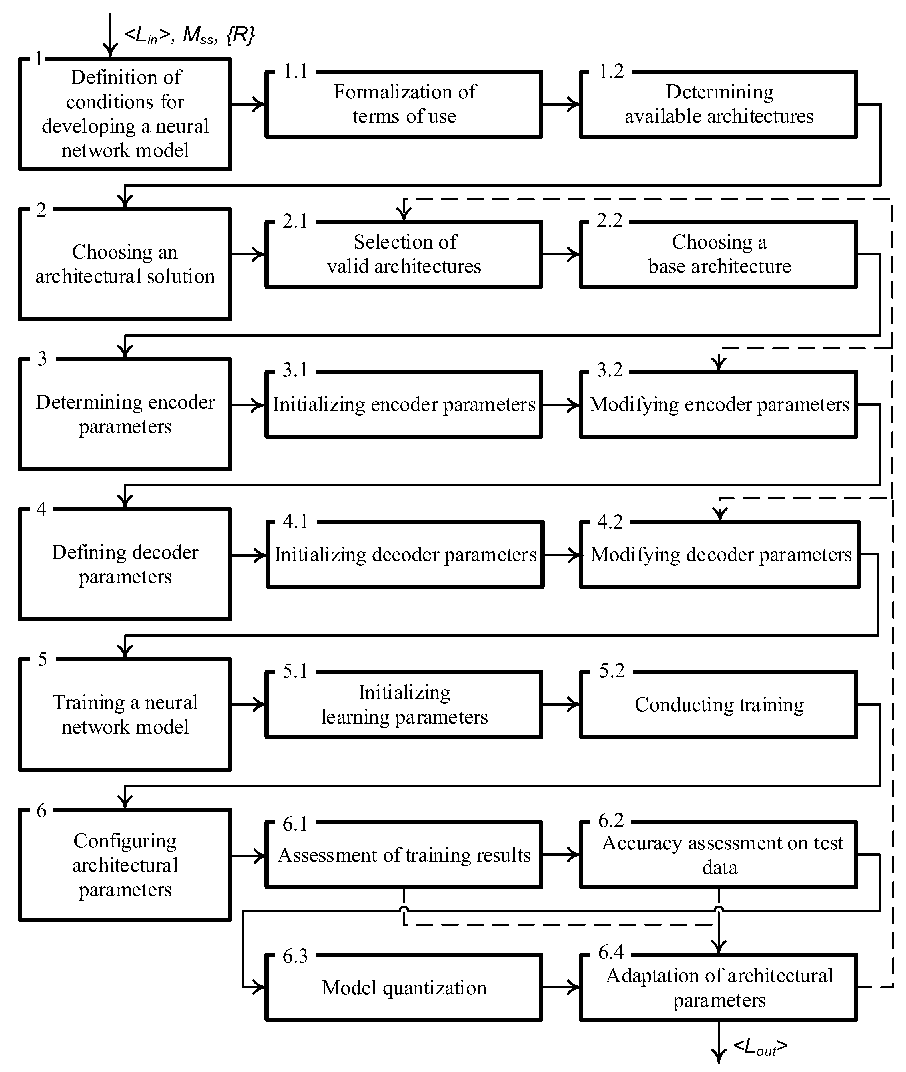
Figure 2.
Graphs of the dependence of Loss and IoU values on the number of training epochs.
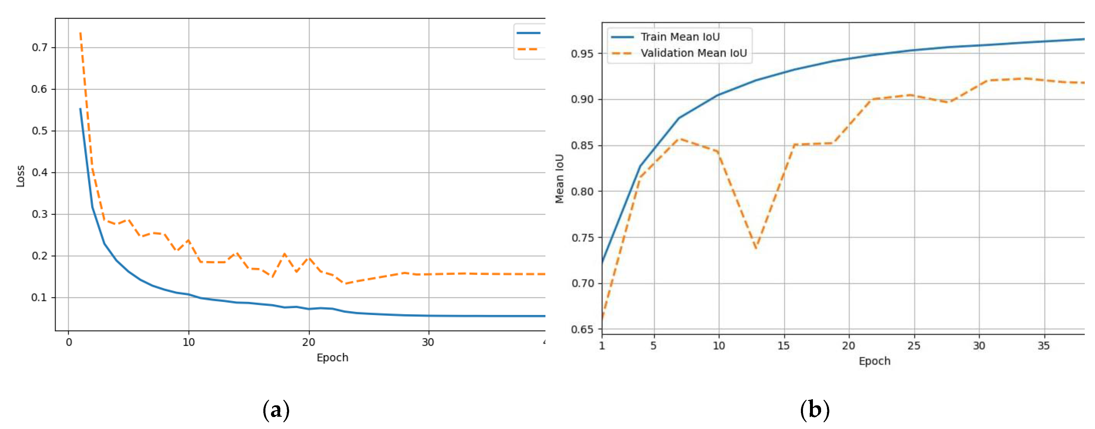
Figure 3.
Visualization of facial image segmentation and processing results.
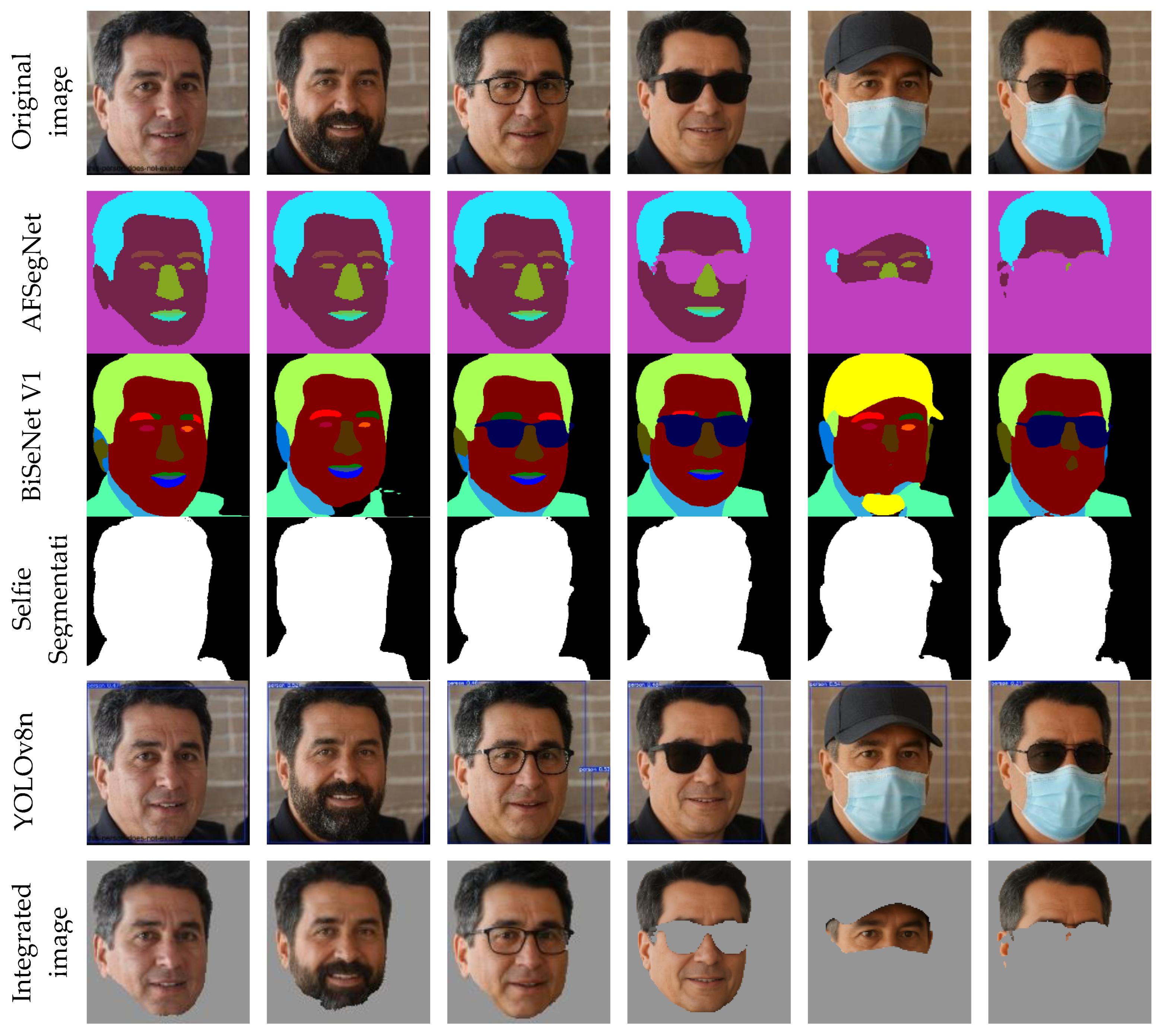

Table 1.
Comparison of face segmentation models.
| Model name | Number of parameters | Segmentation accuracy |
|---|---|---|
| AFSegNet | 0,92 | |
| BiSeNet V1 | 0,83 | |
| Selfie Segmentation | 0,75 |
Disclaimer/Publisher’s Note: The statements, opinions and data contained in all publications are solely those of the individual author(s) and contributor(s) and not of MDPI and/or the editor(s). MDPI and/or the editor(s) disclaim responsibility for any injury to people or property resulting from any ideas, methods, instructions or products referred to in the content. |
© 2025 by the authors. Licensee MDPI, Basel, Switzerland. This article is an open access article distributed under the terms and conditions of the Creative Commons Attribution (CC BY) license (http://creativecommons.org/licenses/by/4.0/).
Copyright: This open access article is published under a Creative Commons CC BY 4.0 license, which permit the free download, distribution, and reuse, provided that the author and preprint are cited in any reuse.


