I. Introduction
Globally, breast cancer continues to be a major cause of cancer-related mortality among women. Early detection and precise diagnosis are essential for enhancing survival rates [
1]. Among various imaging modalities, Breast ultrasound segmentation (BUS) has emerged as a vital tool in clinical practice, due to its non-invasive nature, lack of radiation, and relatively low cost [
2,
3]. However, BUS images are often characterized by strong speckle noise, low contrast, uneven lesion appearance, and blurred boundaries, which pose significant challenges for automatic tumor segmentation in computer-aided diagnosis (CAD) systems.
Deep learning-based segmentation methods have completely transformed BUS image analysis. Architectures such as U-Net [
4] and its variants—including U-Net++ [
5] and Attention U-Net [
6] have achieved remarkable success by leveraging encoder-decoder structures with skip connections. Recently, transformer-based methods and hybrid CNN-state space models have demonstrated outstanding global context modeling capabilities, further enhancing segmentation accuracy. Although they are very effective, these models usually involve a large number of parameters and high computational costs, which limits their practicality in resource-constrained environments, such as portable ultrasound devices used in point-of-care Settings.
To improve efficiency in breast ultrasound segmentation, several studies have adopted lightweight networks that replace heavy backbones with efficient architectures such as MobileNet [
7] and EfficientNet [
8]. While these approaches substantially decrease computational costs, they often suffer from reduced robustness to noise and inadequate delineation of lesion boundaries—a critical aspect in BUS segmentation. Moreover, although attention mechanisms have demonstrated effectiveness in emphasizing salient features and suppressing background interference, prevalent modules tend to introduce considerable computational overhead, hindering their applicability in real-time clinical settings.
Existing BUS segmentation methods therefore face three key limitations. First, heavy models, although achieving high accuracy, are unsuitable for real-time deployment on portable scanners due to their large computational and memory demands. Second, lightweight models often lack sufficient boundary sensitivity and tend to degrade severely on noisy or low-contrast images, which are common in BUS. Third, most existing approaches do not explicitly incorporate boundary priors, even though accurate margin delineation is clinically essential for tumor assessment and treatment planning.
To address these challenges, we propose Lightweight Boundary-Aware Network (LBA-Net) based on the U-Net architecture. It uses a MobileNetV3-Small encoder and an Atrous Spatial Pyramid Pooling (ASPP) bottleneck to capture multi-scale features. The applied Lightweight Boundary-Aware Block (LBA-Block) combines channel and spatial attention to enhance feature discrimination. A boundary-guided decoding scheme injects boundary priors into the decoder to refine skip connections. A dual-head supervision strategy optimizes both segmentation and boundary predictions by a hybrid loss.
The key contributions of this work are as follows:
We propose LBA-Net, a lightweight boundary-aware network for efficiency breast ultrasound image segmentation. By integrating a MobileNetV3 encoder with LBA-Blocks, it achieves high accuracy with minimal computational cost, ideal for resource-constrained environments.
We introduce the Boundary Guidance Module (BGM), which enhances boundary delineation by generating attention maps that guide the decoder, improving lesion boundary accuracy, especially in noisy and low-contrast images.
The Lightweight Boundary-Aware (LBA) Block combines channel and spatial attention mechanisms to refine feature representations, ensuring better sensitivity to key features in ultrasound images.
A dual-head supervision mechanism is proposed, where one head focuses on segmentation and the other on boundary prediction, leading to more precise and stable segmentation results.
III. METHODOLOGY
- A.
Overall Architecture
To achieve a favorable trade-off between segmentation accuracy and computational efficiency, LBA-Net integrates several lightweight strategies into its architecture. First, a MobileNetV3-Small [
25] backbone is adopted as the encoder to extract multi-scale representations. By leveraging depth-wise separable convolutions, squeeze-and-excitation modules, and efficient activation functions, MobileNetV3-Small substantially reduces parameter count and floating-point operations (FLOPs), leading to more than 90% reduction in complexity compared with conventional U-Net encoders.
Second, we introduce the LBA-Block, which enhances feature discriminability with negligible computational overhead. Unlike conventional attention modules that rely on heavy convolutions and fully connected layers, the LBA-Block fuses two lightweight components: (i) ECA, which models cross-channel interactions through a 1D convolution without dimensionality reduction, thereby avoiding parameter inflation; and (ii) spatial attention based on a 3×3 depth-wise separable convolution, which highlights salient spatial regions. Moreover, we introduce adaptive fusion weights (α, β) to dynamically balance the contributions of channel and spatial attention, allowing the model to emphasize either modality depending on the input context.
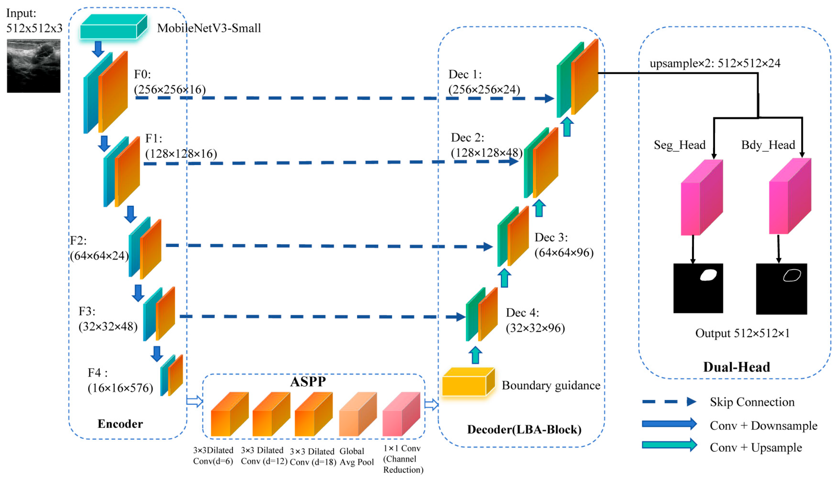
Finally, the decoder adopts streamlined skip connections and incorporates a dual-head supervision scheme. This design not only facilitates precise boundary localization but also maintains a compact model size by avoiding redundant layers. LBA-Net adopts an encoder–decoder architecture with skip connections, following the U-Net paradigm. The overall pipeline consists of four main components (
Figure 1):
The proposed network is built upon a lightweight encoder-decoder framework. A pre-trained MobileNetV3-Small model is adopted as the encoder to extract hierarchical multi-scale features {
F0,
F1, F2, F3, F4} at progressively reduced spatial resolutions. At the bottleneck, the ASPP module [
13] is incorporated to capture multi-scale contextual information over diverse receptive fields. In the decoder path, feature maps are gradually upsampled and fused with corresponding encoder features via skip connections. At each stage of the decoder, a Lightweight Boundary-aware block is applied to enhance discriminative feature learning while suppressing irrelevant background responses. Furthermore, the network employs a dual-head output structure: one head produces the segmentation mask, while the other generates a boundary map. In the decoder path, feature maps are progressively upsampled and fused with encoder features via skip connections. At the bottleneck, an ASPP module first produces multi-scale features, which are further transformed by a boundary guidance module into a boundary attention map. This attention is injected into the first decoder block, where it modulates the corresponding skip feature through a learnable guidance branch, enhancing responses along potential lesion boundaries while suppressing background noise.
At each decoding stage, an LBA-Block refines the fused features via lightweight channel–spatial attention. After the final decoder layer, a dual-head output structure is employed: one head predicts the segmentation mask and the other predicts a boundary probability map, both from the same decoded feature representation. The boundary head is supervised by edge labels obtained from morphological gradients of the ground-truth masks, and a consistency loss additionally aligns the internal boundary attention map with these edge labels. Notation: Given an input ultrasound image
, the backbone produces a feature map
. All feature maps in this paper follow the convention where
C, H, and
W denote the channel, height and width, respectively.
|
Algorithm 1: Main structure of LBA-Net |
Input: I ∈ R^(H×W×C)
Output: Segmentation mask S, boundary map B, total loss L_total
1: {F0, F1, F2, F3} ← ENCODER(I)
2: F_aspp ← ASPP_MODULE(F4)
3: A_b ← BOUNDARY_GUIDANCE(F_aspp)
4: X_dec ← DECODER(F_aspp, {F3, F2, F1, F0}, A_b)
5: S, B, S_logits, B_logits ← HEADS(X_dec)
6: L_total ← LOSS(S_logits, B_logits, A_b, G, Bgt)
7: return S, B, L_total |
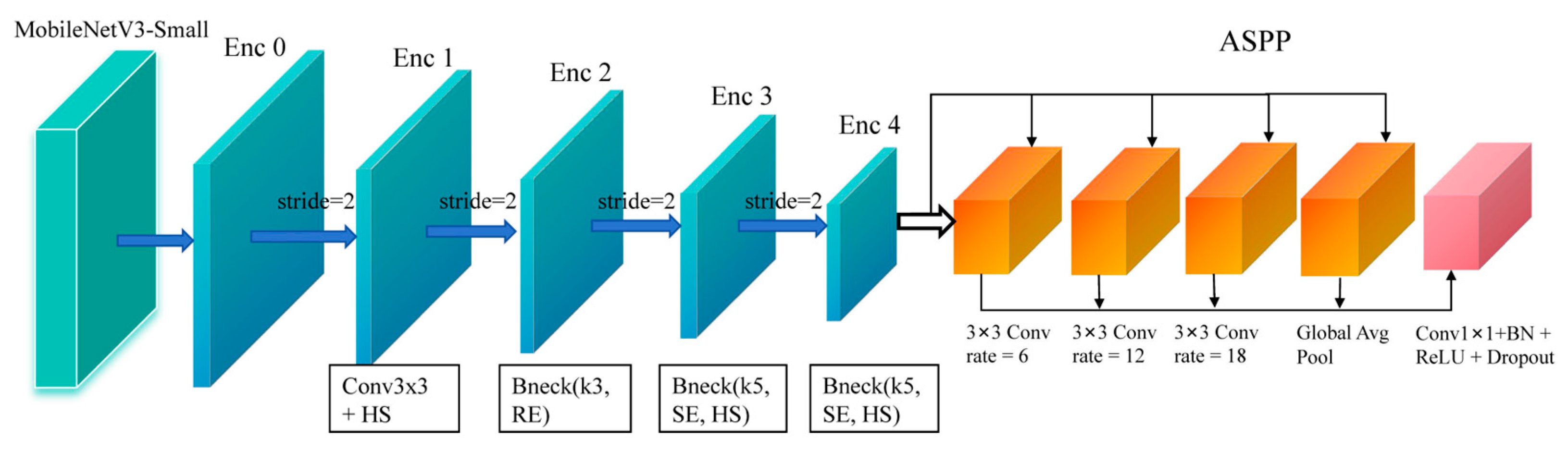
The overall encoder configuration is illustrated in
Figure 2. To efficient extract discriminative representations from ultrasound images, the encoder of LBA-Net adopts MobileNetV3 as the backbone due to its lightweight and high-performance design. The backbone generates a hierarchical feature maps {
F0,F1,F2,F3,F4} through multiple inverted residual bottlenecks with stride-2 downsampling. Compared to conventional convolutions, the inverted residual structure with depth-wise separable convolution significantly reduces computation overhead while preserving local semantic features. Additionally, MobileNetV3 incorporates squeeze-and-excitation (SE) and hard-swish (HS) activation, which enhance channel dynamics and nonlinear capacity, respectively, thus improving robustness against ultrasound noise and artifacts.
However, breast tumors often exhibit large scale variations and blurred boundaries, which require sufficient receptive field. To address this issue, the highest-level feature
F4 is fed into an ASPP module for enlarged multi-scale context aggregation. ASPP consists of four parallel branches: a 1×1 convolution, three 3×3 dilated convolutions with dilation rates {6, 12, 18}, and a global average pooling branch. The outputs are concatenated and projected to form an enhanced representation with rich local–global context:
where
denotes concatenation followed by a 1×1 projection.
To extract multi-scale features with high discriminative power while minimizing computational overhead, we adopt MobileNetV3-Small.
(a) Channel Attention
Given feature map
, we apply ECA or a squeeze-excitation (SE) mechanism:
where GAP denotes global average pooling, Conv1D is a 1D convolution with kernel size k, and σ is the sigmoid function.
The channel-refined feature is:
where ⊗ denotes channel-wise multiplication.
(b) Spatial Attention
Spatial attention focuses on salient regions using depth-wise separable convolution:
where depth-wise separable convolution is with kernel size 3×3.
The spatially refined feature is:
(c) Fusion
The final output is obtained by combining both attentions:
where α and β are learnable scalar weights initialized as 0.5.
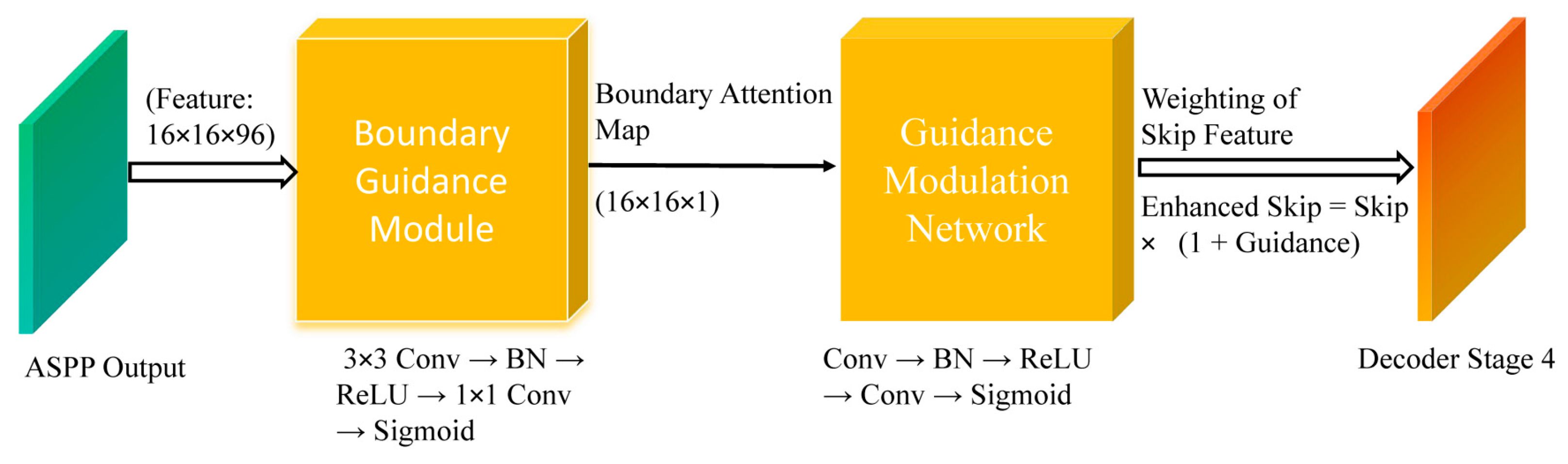
Ultrasound images often present weak and ambiguous lesion boundaries. To explicitly inject boundary priors into the decoder for sharper lesion delineation.
Figure 3 illustrates the Boundary Guidance Module (BGM). The ASPP feature is first transformed by a lightweight convolutional branch to generate an attention map highlighting potential tumor boundaries. This attention is then injected into the skip connection of the first decoder stage using a modulation network, allowing boundary cues to influence early decoding where spatial details are most critical.
- (a)
Boundary Guidance Modulation
Given the ASPP feature
Faspp∈RC×H×W, BGM predicts a boundary-attention map through a compact convolutional subnetwork:
Where denotes the sigmoid function
Let
G(
Fb) represent the modulation weight obtained from the boundary attention map
Fb :
let
Fskip∈
RB×Cskip×H×W represent the skip connection feature map from the decoder, where
Cskip is the number of channels in the skip connection. For each input, the boundary-guided feature modulation is applied as follows:
where
Fskip is the skip connection feature map.
where is the ground-truth boundary map derived from the segmentation mask, and Up(⋅) indicates bilinear upsampling to the original image size.
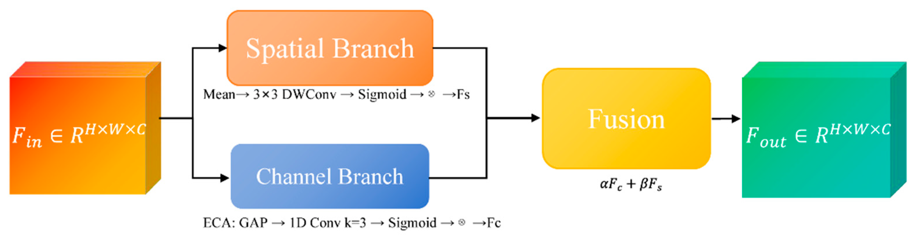
To enhance feature discriminability while maintaining computational efficiency, we propose the Lightweight Boundary-aware Attention Block, an attention module that adaptively refines feature representations by fusing channel-wise and spatial-wise attention mechanisms with minimal parameter overhead. Unlike conventional attention modules that rely on dense convolutions and global pooling operations, the LBA-Block is specifically designed for edge deployment in resource-constrained clinical environments.
As illustrated in
Figure 4, LBA-Block first reweights channels via ECA [
26], then generates a 3×3 depth-wise spatial attention map, and finally fuses both branches through learnable α, β to yield the refined feature.
(a) Channel Branch
Channel attention aims to recalibrate feature channels by emphasizing informative responses and suppressing less useful ones. We adopt the ECA mechanism due to its parameter-free design and strong performance in low-resource settings. Given input
Fin∈RC×H×W, global average pooling (GAP) is first applied to produce channel-wise descriptors:
where
Zc represents the mean activation of channel
c.
A 1D convolution with kernel size k (set to 3 in our implementation) is then applied to capture cross-channel interactions without dimensionality reduction:
where σ denotes the sigmoid activation function. The channel-refined feature
Fc is obtained via channel-wise multiplication:
This design eliminates channel dimensionality reduction and significantly reduces parameters while effectively modeling inter-channel dependencies.
(b) Spatial Branch
Spatial attention focuses on identifying salient regions within each feature map. To minimize computational cost, we employ depth-wise separable convolution with a 3×3 kernel instead of standard convolutions or large-kernel spatial attention. The spatial attention map
As is computed as:
where
DWConv denotes depth-wise convolution followed by point-wise projection to a single channel. The spatially refined feature
Fs is then:
This lightweight design substantially reduces the spatial attention computation while effectively preserving fine-grained lesion boundaries and suppressing background clutter in ultrasound images.
(c) Adaptive Fusion
To effectively integrate semantic enhancement from the channel branch and boundary refinement from the spatial branch, we introduce learnable fusion weights
α and
β, initialized to 0.5 and jointly optimized in an end-to-end manner:
This adaptive strategy enables the network to dynamically emphasize channel semantics in noisy regions, or spatial boundary cues in low-contrast tumor edges, while keeping computational overhead negligible.
As illustrated in
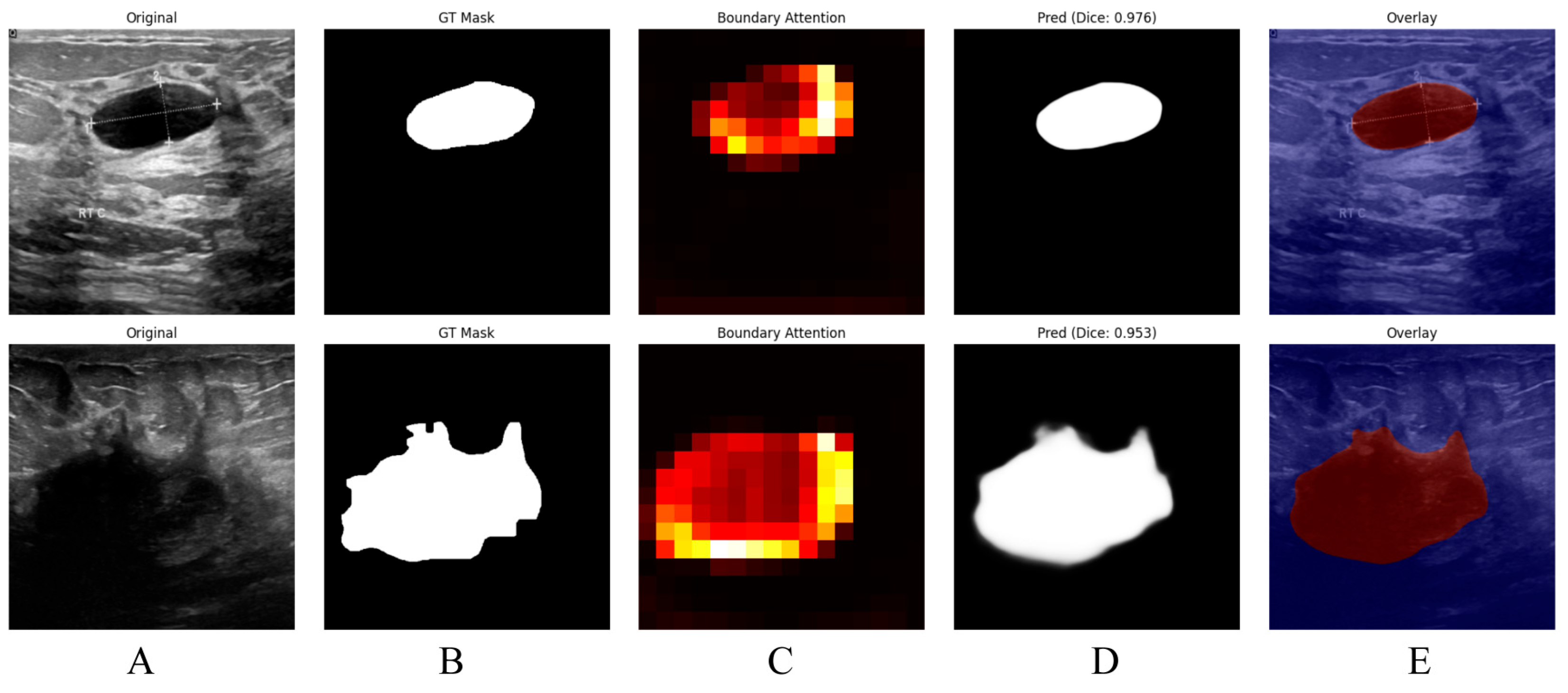
Figure 5, the proposed boundary-aware attention mechanism yields accurate and visually coherent breast lesion segmentation results in ultrasound images. The original images in Column (A) contain lesions with complex textures and heterogeneous backgrounds, while the corresponding ground truth masks in Column (B) provide precise lesion annotations. The boundary-attention heatmaps shown in Column (C), together with the predicted masks in Column (D), indicate that the model effectively concentrates on lesion boundaries and produces accurate delineations, achieving Dice scores of 0.976 and 0.953. Moreover, the overlay images in Column (E), obtained by superimposing the predicted masks onto the original images, intuitively demonstrate the spatial consistency between the predictions and the underlying anatomy, thereby further confirming the effectiveness of the proposed model in delineating breast lesions in ultrasound images.
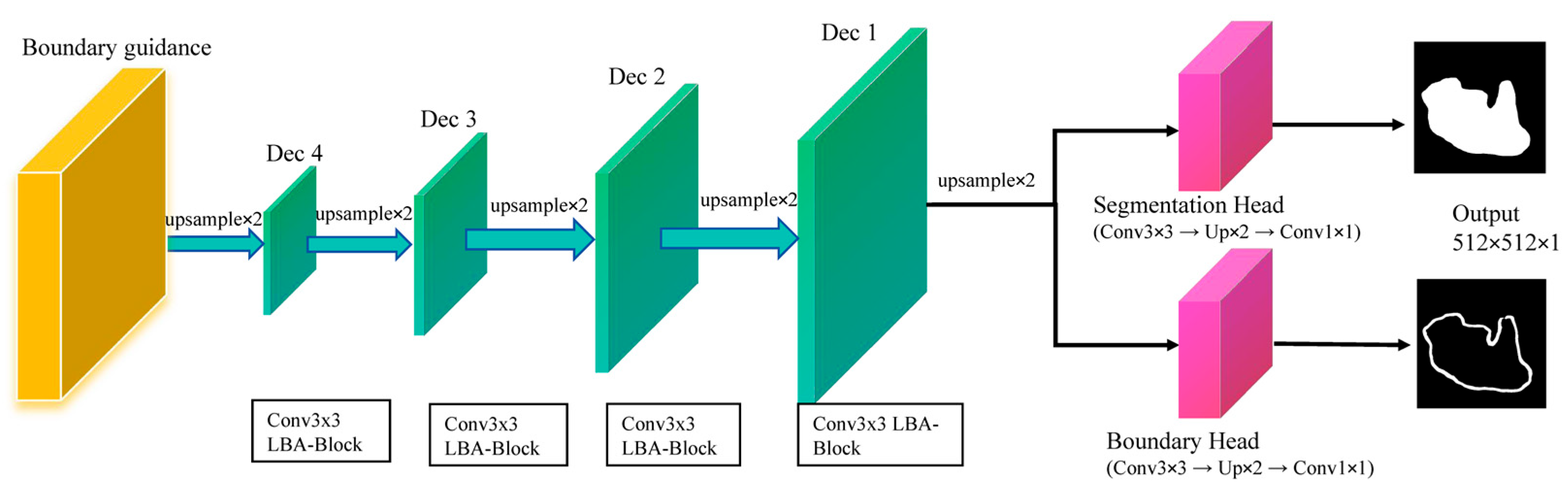
To enhance boundary delineation in ultrasound segmentation, LBA-Net adopts a dual-head architecture in
Figure 6:
LBA-decoder: four-step upsampling of multi-scale encodings (Dec1-Dec4) to dual-head outputs; segmentation logits S refined by 3×3 weight Wb inferred from boundary logits B; losses: Dice+BCE on S, Tversky on B.
- (a)
Segmentation Head:
Outputs a binary segmentation maskwhere denotes the spatial resolution of the input image which consistent with the 512×512 input size. A pixel value of 1 represents the tumor region, while 0 represents the background which are normal breast tissue or artifacts.
Outputs a probability map
highlighting object boundaries, with ground-truth labels derived via morphological gradient operations on
Sgt. The boundary labels are computed as:
where
and
denote morphological dilation and erosion, respectively. The subtraction result is then binarized to ensure a consistent supervision target:
The overall training objective combines segmentation loss, boundary loss, and a boundary-consistency term:
where
supervises the mask predictions,
supervises the boundary head, and
enforces consistency between the internal boundary attention and the morphology-derived boundary labels. In our implementation, we set λ
bdy=0.3 and λ
cons=0.1.
- (a)
Segmentation Loss:
Where (Binary Cross-Entropy Loss) measures pixel-wise differences between the predicted mask Slogits and the ground-truth mask , and (Dice Loss) evaluates the overlap between the predicted and ground-truth masks, which is especially useful for handling class imbalance between foreground and background pixels.
We adopt Tversky loss to address class imbalance in boundaries:
where TP, FP, FN are the numbers of true positives, false positives, and false negatives along the boundary. We set
α=0.3 and
β=0.7 to emphasize recall, penalizing false negatives more strongly.
Finally, we encourage the boundary attention map
Ab predicted by the boundary guidance module to be consistent with
Bgt via a mean squared error(MSE):
where the attention map is interpolated to the resolution of the boundary labels. This term links the implicit attention in the encoder–decoder with the explicit boundary supervision, leading to sharper and more stable boundary predictions.
To comprehensively assess segmentation performance, four commonly used metrics are employed:
where
and
denote the predicted and ground-truth tumor regions,
denotes the Euclidean distance,
perc95 represents the 95th percentile. Lower HD95 indicates better boundary accuracy. A smaller HD95 indicates closer spatial agreement between the predicted and ground-truth boundaries, corresponding to higher boundary accuracy. HD95 is reported in pixel units since physical pixel spacing was unavailable; thus the value should be interpreted as a relative metric. Furthermore, we chose the model's parameter count and computational cost (GFLOPs) as critical metrics to evaluate the balance between its lightweight design and performance.
All images are resized to 512×512, normalized using ImageNet statistics, and augmented with random horizontal flips (0.5), vertical flips (0.3), ±30° rotations, brightness–contrast adjustment, and 3×3 Gaussian blur. Training is performed using mixed-precision (FP16) with a batch size of 24 and gradient clipping for optimization stability. We employ the AdamW [
27] optimizer with module-specific learning rates: 1×10
−4 for the MobileNetV3 backbone, 2×10
−3 for the decoder, and 3×10
−3 for the boundary-guidance and head modules. A One-Cycle learning rate schedule is used over 300 epochs, consisting of a 10% warm-up phase followed by cosine decay. The MobileNetV3-Small encoder is initialized with ImageNet pre-trained weights.
IV. Experiments
- A.
Datasets
We evaluated LBA-Net on the publicly available breast ultrasound dataset. The first dataset was the BUSI dataset [
28] contains 780 images, including 437 benign cases, 210 malignant cases and 133 normal cases, and the second dataset utilized in this study was established at the medical center of the Bangladesh University of Engineering and Technology (BUET) [
29], Dhaka, Bangladesh, between 2012 and 2013. Breast ultrasound data were acquired using a Sonix-Touch Research system equipped with a linear L14-5/38 transducer, operating at a center frequency of 10 MHz and a sampling frequency of 40 MHz. It comprises 260 images from 223 female patients (aged 13–75 years), including 190 benign and 70 malignant cases. The image resolutions vary from 298 × 159 to 800 × 600 pixels. Each image is accompanied by pixel-level truth segmentation masks from multiple patients.
A chief physician with 15 years of experience in radiology and a attending physician with 3 years of experience in radiology independently read the films using a double-blind method. According to the ACR TI-RADS quality clause, the original ultrasound sequences were scored at five levels. Only cases with a score ≥ 4 and the two agreed (k = 0.87) were retained. The differences were arbitrated by chief physicians with 15 years of experience. Eventually, as shown in
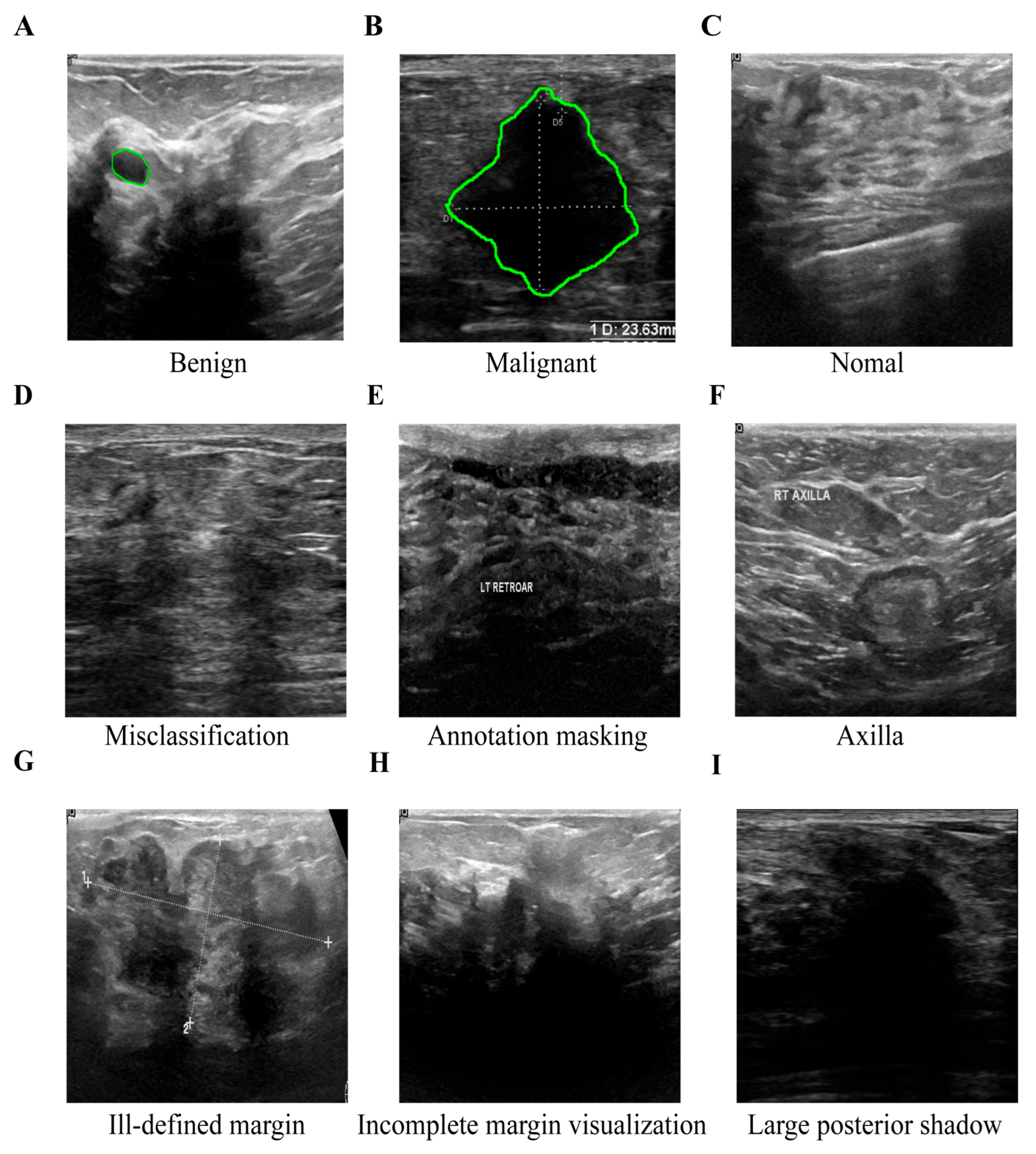
Figure 7, their assessment identified a subset of low-quality breast ultrasound images, which exhibited issues including misclassification, text overlay obscuring tissue, the presence of axillary tissue, indistinct lesion boundaries, and substantial acoustic shadowing. These examples demonstrate typical failure cases where reliable annotation is impossible, justifying their exclusion during dataset curation.
We selected 570 cases (380 benign, 190 malignant) from BUSI and 230 cases (174 benign, 56 malignant) from BUET for our analysis. To ensure clarity and comparability, these quality-screened subsets are denoted as BUSI* and BUET* throughout this paper, with the asterisk symbol (*) in tables and figures indicating the curated datasets used in this study.
All experiments are implemented in PyTorch 1.12 and conducted on an NVIDIA GeForce RTX 4090 D GPU (25 GB) with TensorRT and Automatic Mixed Precision (AMP) enabled, as well as a Core i7-14700KF CPU (3.40 GHz). Notably, all comparative models are also subject to the same TensorRT acceleration and AMP settings to ensure fair performance comparison. Model efficiency is evaluated in terms of parameters, FLOPs, and inference speed on both the aforementioned GPU and CPU. Segmentation performance is assessed using Dice, IoU, precision, recall, and HD95. For both BUSI* and BUET* datasets, we adopt 5-fold stratified cross-validation with identical preprocessing and evaluation protocols across all folds.
As summarized in
Table 1, the proposed LBA-Net achieves strong segmentation performance on BUSI, BUSI*, BUET, and BUET*, with the refined subsets (BUSI* and BUET*) yielding notably higher Dice, IoU, and Recall scores as well as substantially lower HD95 values. These improvements highlight the advantages of higher-quality annotations and demonstrate the model’s ability to produce more accurate and reliable lesion boundary localization across datasets of varying complexity.
To comprehensively evaluate the effectiveness of the proposed LBA-Net, we compare it with several state-of-the-art CNN-based segmentation models, including UNet, UNet++, FPN, DeepLabv3+, AttentionUNet, SegNet, and ResUNet.
Table 2 and
Table 3 summarize the quantitative results on the BUSI* and BUET* datasets at an input resolution of 512×512.
- (a)
Performance on the BUSI*
On the BUSI* dataset, LBA-Net achieves a Dice score of 83.35% and IoU of 76.49%, which are competitive with or better than most CNN-based baselines. While DeepLabv3+ achieves a slightly higher Dice score (84.96%), LBA-Net surpasses all models in terms of efficiency, requiring only 3.34 GFLOPs and 1.76M parameters, which are dramatically lower than all competing architectures. The HD95 of LBA-Net (38.02 px) is also significantly better than most classical CNN models and substantially better than heavy architectures such as AttentionUNet, SegNet, and ResUNet.
In addition, LBA-Net achieves 123.43 FPS on GPU and 19.42 FPS on CPU, far exceeding all CNN-based baselines. This indicates that LBA-Net maintains strong segmentation accuracy while being exceptionally lightweight and fast, making it suitable for real-time or resource-constrained clinical applications.
The performance trend on BUET* is consistent with that on BUSI*. LBA-Net again delivers a strong balance between segmentation accuracy and computational efficiency. Although DeepLabv3+ records the highest Dice score (87.42%), LBA-Net maintains competitive performance with a Dice score of 86.59%, while requiring up to 10×–70× fewer FLOPs and 10–20× fewer parameters than traditional CNN architectures.
Furthermore, LBA-Net preserves its extremely high inference speed across hardware platforms, obtaining 123.43 GPU FPS and 19.42 CPU FPS, which are significantly higher than all state-of-the-art competitors. This demonstrates that LBA-Net not only performs efficiency on different ultrasound datasets but also generalizes well with consistently low latency and minimal computational overhead.
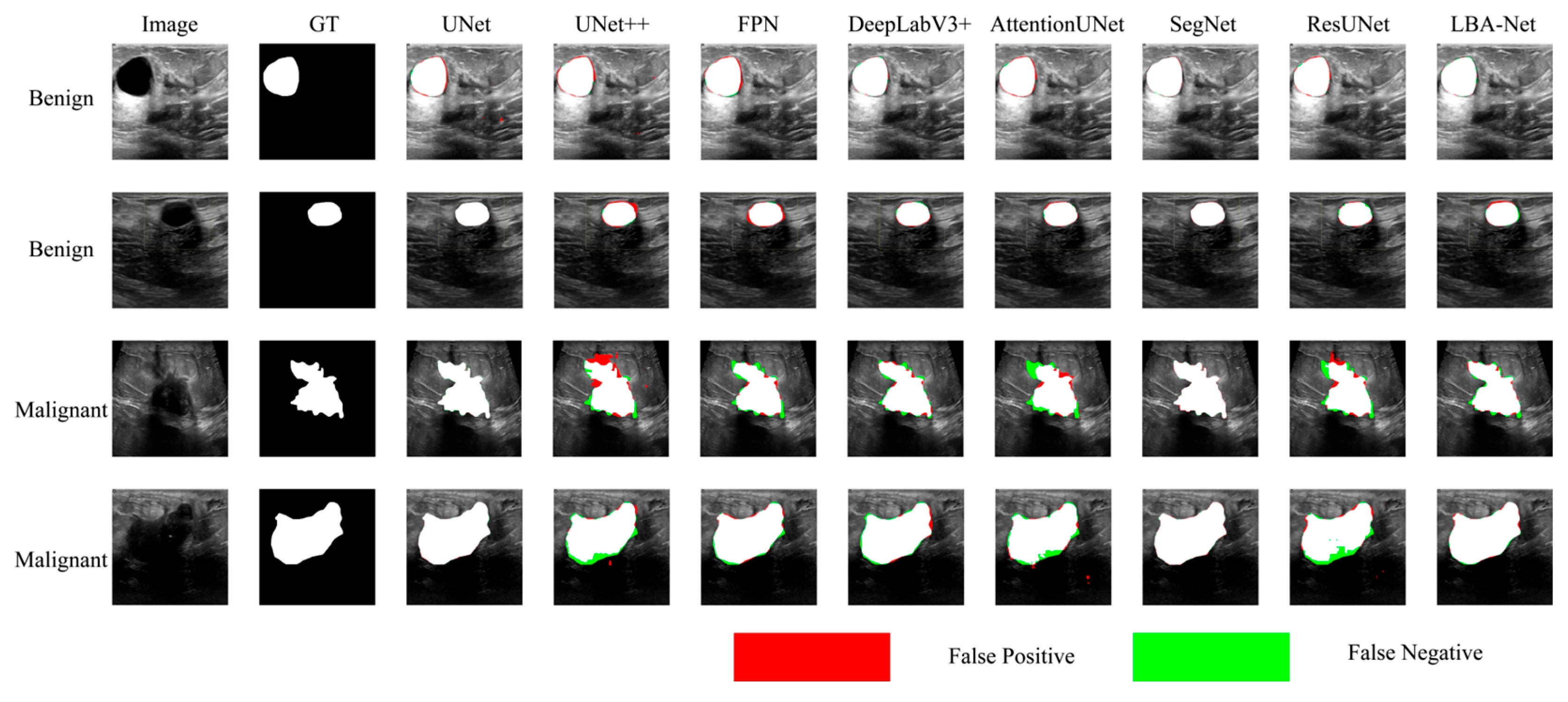
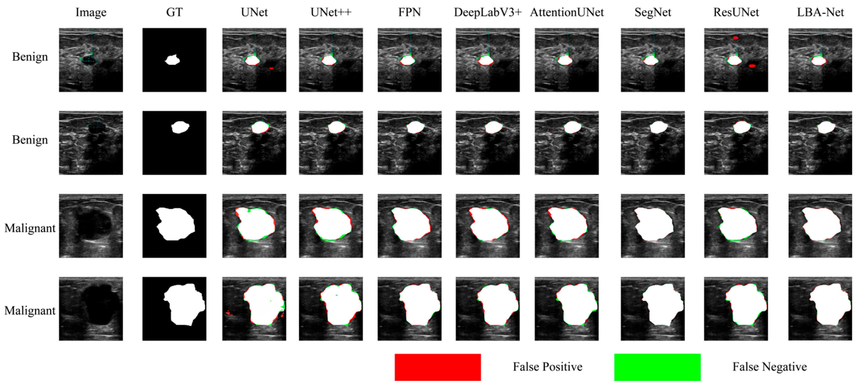
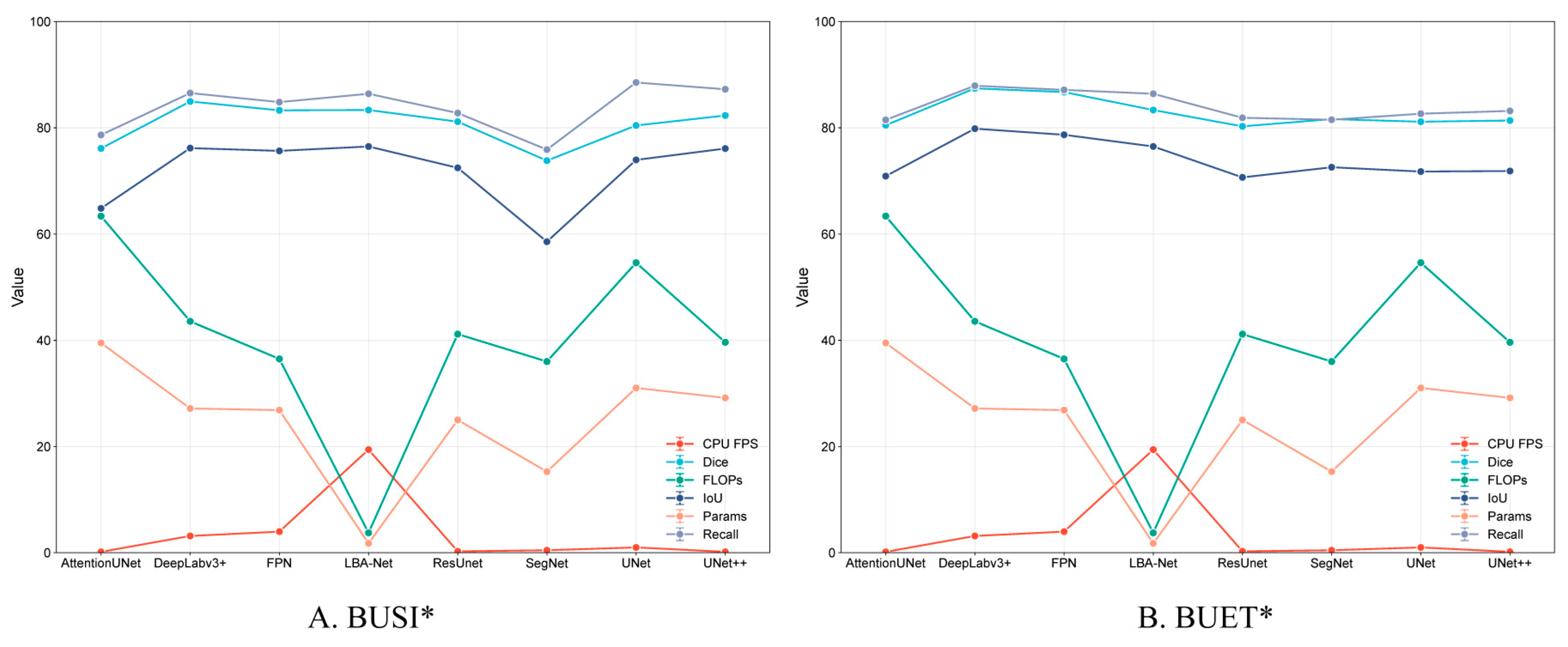
Figure 8 and
Figure 9 compare segmentation outputs across different CNN architectures. LBA-Net consistently produces masks that adhere more closely to ground-truth boundaries, particularly in low-contrast or irregular-shaped tumors. Competing models such as SegNet and ResUNet tend to produce over-segmented or under-segmented results, as highlighted by the false-positive (red) and false-negative (green) regions. As shown in
Figure 10, LBA-Net attains competitive Dice and IoU scores while exhibiting the lowest computational cost (FLOPs) and the highest inference speed (FPS) among all compared methods. Such a favorable accuracy–efficiency trade-off underscores its suitability for real-time clinical deployment, particularly on resource-constrained ultrasound devices.
To quantitatively validate the contribution of each design in LBA-Net, we performed a lightweight yet complete ablation study on the BUSI* dataset. Starting from the full model, we progressively ablated or substituted the key components, resulting in five configurations:
(1) Full (LBA-Net): all proposed modules are active.
(2) w/o Boundary Guidance: The boundary guidance module is removed, but the LBA-Blocks and boundary head (with boundary loss and consistency loss) remain.
(3) w/o Boundary Head (Single-head): The boundary head is removed, leaving only the segmentation head, without boundary loss or consistency loss.
(4) w/o Boundary-Consistency Loss: The boundary-consistency loss is removed, but both segmentation and boundary heads are trained with their respective losses.
(5) w/o LBA-Block: LBA-Blocks are replaced with standard SE-enhanced convolutions, with ASPP, boundary guidance, and dual-head supervision retained
(6) w/o ASPP: The ASPP module is removed, and the deepest encoder feature is directly passed to the decoder without multi-scale context aggregation.
All models were trained under identical hyper-parameters (512×512 input, 300 epochs, AdamW, cosine LR), without test-time augmentation.
To quantify the contribution of each component in LBA-Net, we performed a series of ablation experiments by removing one module at a time, as reported in
Table 4 and visualized in
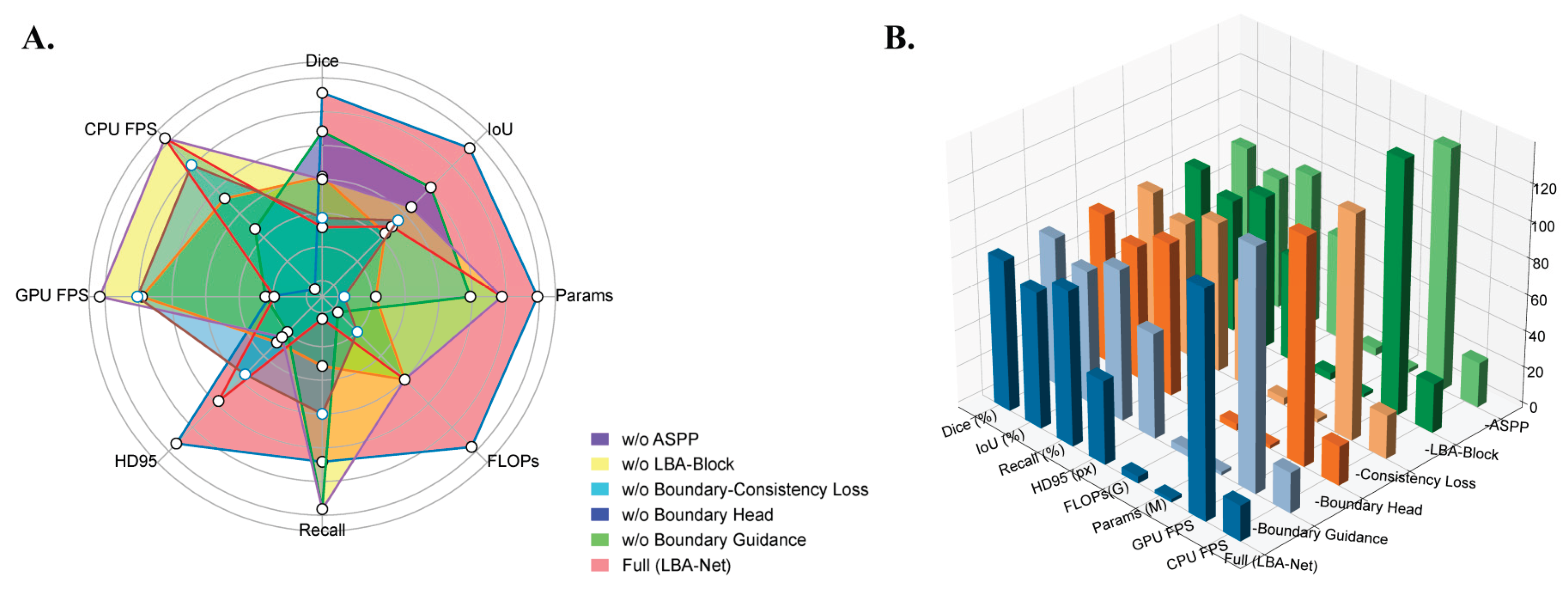
Figure 11. The results show that each component contributes to both accuracy and boundary stability.
Removing the Boundary Guidance Module leads to a noticeable degradation in segmentation quality, with Dice dropping from 82.79% to 82.02% and HD95 increasing by +11.7 px. This trend, clearly reflected in the radar chart in
Figure 11A, demonstrates that injecting boundary priors at an early decoding stage is crucial for restoring sharper lesion margins under ultrasound noise.
The single-head variant (without the Boundary Head) shows a similar deterioration pattern (Dice 82.12%, HD95 +12.4 px), indicating that explicit boundary supervision provides stable structural cues that complement mask prediction. Meanwhile, removing the Boundary-Consistency Loss produces the largest Dice reduction among boundary-related components (−1.03%), as seen in both
Table 4 and
Figure 11B, confirming that enforcing consistency between implicit attention and morphology-derived boundaries is essential for precise edge recovery.
Eliminating the LBA-Block also decreases boundary accuracy substantially (HD95 +12.2 px), highlighting the importance of lightweight channel–spatial attention for refining local features, particularly in low-contrast or fuzzy regions typical of breast ultrasound.
Finally, removing the ASPP module yields the lowest Dice score (81.81%) and increases the model size, as the multi-branch dilated convolutions are replaced by standard convolutions. This demonstrates that multi-scale context aggregation is necessary for capturing lesions of varying sizes and shapes.
Overall, both
Table 4 and
Figure 11 consistently show that the full LBA-Net achieves the most balanced performance across Dice, IoU, HD95, FLOPs, and inference speed, validating the complementary roles of all proposed components.
Figure 1.
The structure diagram of LBA-Net.
Figure 1.
The structure diagram of LBA-Net.
Figure 2.
Encoder structure of LBA-Net using MobileNetV3 backbone and ASPP module.
Figure 2.
Encoder structure of LBA-Net using MobileNetV3 backbone and ASPP module.
Figure 3.
Boundary Guidance structure.
Figure 3.
Boundary Guidance structure.
Figure 4.
LBA-Block structure. Structure of the proposed Lightweight Boundary-aware Attention Block, consisting of channel attention, spatial attention, and adaptive fusion modules.
Figure 4.
LBA-Block structure. Structure of the proposed Lightweight Boundary-aware Attention Block, consisting of channel attention, spatial attention, and adaptive fusion modules.
Figure 5.
Visualization of Breast Lesion Segmentation Results in Ultrasound Images with Boundary-Aware Attention by using the BUSI. This Figure shows breast lesion segmentation results in ultrasound images using a boundary-aware attention model.A (Original): Original ultrasound images.B (GT Mask): Ground truth lesion masks. C (Boundary Attention): Heatmaps of boundary attention (warmer colors = high boundary focus). D (Pred): Predicted segmentation masks with Dice similarity coefficient. F (Overlay): Predicted masks overlaid on original images. Two cases are presented, with Dice scores of 0.976 and 0.953, illustrating accurate lesion delineation.
Figure 6.
LBA-Block powered decoder with dual-head boundary-aware prediction.
Figure 6.
LBA-Block powered decoder with dual-head boundary-aware prediction.
Figure 7.
Example of some sub-optimal images from the BUSI and BUET datasets. To ensure data quality, images exhibiting critical flaws were excluded from this study and the green circle indicates GT mask. The retained training images (A-C) show clinically validated, high-resolution examples of benign, malignant, and normal breast tissues. The excluded problematic images (D-I) illustrate specific exclusion criteria: (D) misclassification, (E) text occlusion, (F) inclusion of irrelevant axillary tissue, (G) indistinct boundaries, (H) missing boundaries, and (I) extensive acoustic shadowing.
Figure 8.
Comparison of Segmentation Results onBUSI* datasets.
Figure 8.
Comparison of Segmentation Results onBUSI* datasets.
Figure 9.
Comparison of Segmentation Results onBUET* datasets.
Figure 9.
Comparison of Segmentation Results onBUET* datasets.
Figure 10.
Performance Comparison of Segmentation Models on BUSI* and BUET* Datasets.
Figure 10.
Performance Comparison of Segmentation Models on BUSI* and BUET* Datasets.
Figure 11.
Visualization of LBA-Net ablation study results: A. Radar comparison across Dice, IoU, Recall, HD95, FLOPs, Params, GPU FPS, and CPU FPS; B. 3D bar chart illustrating metric differences among ablated variants.
Figure 11.
Visualization of LBA-Net ablation study results: A. Radar comparison across Dice, IoU, Recall, HD95, FLOPs, Params, GPU FPS, and CPU FPS; B. 3D bar chart illustrating metric differences among ablated variants.
Table 1.
Quantitative comparison of segmentation performance on the BUSI, BUSI*, BUET, and BUET* datasets.
Table 1.
Quantitative comparison of segmentation performance on the BUSI, BUSI*, BUET, and BUET* datasets.
| Dataset |
Dice (%) |
IoU (%) |
Recall(%) |
HD95(px) |
| BUSI |
78.39 ± 2.43 |
69.52 ± 2.57 |
79.35 ± 2.51 |
67.81 ± 6.94 |
| BUSI* |
82.79 ± 2.48 |
74.96 ± 2.43 |
85.02 ± 2.09 |
45.96 ± 9.82 |
| BUET |
83.93 ± 1.59 |
74.86 ± 1.88 |
84.82 ± 1.79 |
63.27 ± 8.54 |
| BUET* |
86.59 ± 1.87 |
77.92 ± 1.52 |
87.54 ± 1.38 |
52.60 ± 7.35 |
Table 2.
Performance comparison of each model on the BUSI* dataset@ 512×512 Input.
Table 2.
Performance comparison of each model on the BUSI* dataset@ 512×512 Input.
| Model Category |
Model Name |
Dice (%) |
IoU (%) |
Recall(%) |
HD95(px) |
FLOPs (G) |
Params (M) |
GPU FPS |
CPU FPS |
| CNN-based |
UNet |
80.44 ± 1.65 |
73.96 ± 1.58 |
88.53± 1.77 |
23.86 ± 2.15 |
54.61 |
31.03 |
34.98 |
0.99 |
| CNN-based |
UNet++ |
82.32 ± 1.68 |
76.10 ± 1.62 |
87.26 ± 1.74 |
19.69 ± 1.97 |
39.63 |
29.16 |
32.60 |
0.17 |
| CNN-based |
FPN |
83.29 ± 2.70 |
75.66 ± 2.60 |
84.84 ± 1.70 |
50.99 ± 3.06 |
36.50 |
26.85 |
136.77 |
3.97 |
| CNN-based |
DeepLabv3+ |
84.96 ± 1.61 |
76.18 ± 3.24 |
86.54 ± 1.61 |
50.54 ± 6.29 |
43.57 |
27.17 |
108.51 |
3.15 |
| CNN-based |
AttentionUNet |
76.12 ± 2.58 |
64.84 ± 2.42 |
78.66 ± 1.57 |
82.13 ± 4.93 |
63.38 |
39.51 |
28.65 |
0.16 |
| CNN-based |
SegNet |
73.82 ± 1.54 |
58.57 ± 1.35 |
75.90 ± 1.52 |
97.61 ± 5.86 |
36.01 |
15.27 |
46.24 |
0.46 |
| CNN-based |
ResUnet |
81.16 ± 1.66 |
72.47 ± 1.55 |
82.78 ± 1.66 |
64.61 ± 3.88 |
41.17 |
25.01 |
69.15 |
0.26 |
| Proposed |
LBA-Net |
83.35 ± 2.42 |
76.49 ± 1.55 |
86.41 ± 1.73 |
38.02 ± 2.66 |
3.74 |
1.76 |
123.43 |
19.42 |
Table 3.
Performance comparison of each model on the BUET* dataset@ 512×512 Input.
Table 3.
Performance comparison of each model on the BUET* dataset@ 512×512 Input.
| Model Category |
Model Name |
Dice (%) |
IoU (%) |
Recall (%) |
HD95(px) |
FLOPs (G) |
Params (M) |
GPU FPS |
CPU FPS |
| CNN-based |
UNet |
81.15 ± 3.46 |
71.77 ± 4.26 |
82.66 ± 3.23 |
86.57 ± 18.52 |
54.61 9 |
31.03 |
34.98 |
0.99 |
| CNN-based |
UNet++ |
81.38 ± 3.59 |
71.87 ± 4.42 |
83.18 ± 2.35 |
91.77 ± 18.18 |
39.63 |
29.16 |
32.60 |
0.17 |
| CNN-based |
FPN |
86.73 ± 2.16 |
78.69 ± 2.55 |
87.14 ± 2.76 |
43.97 ± 7.85 |
36.50 |
26.85 |
136.77 |
3.97 |
| CNN-based |
DeepLabv3+ |
87.42 ± 2.78 |
79.84 ± 3.21 |
87.92 ± 3.71 |
38.12 ± 7.21 |
43.57 |
27.17 |
108.51 |
3.15 |
| CNN-based |
AttentionUNet |
80.49 ± 3.40 |
70.91 ± 4.02 |
81.49 ± 3.73 |
89.86 ± 14.93 |
63.38 |
39.51 |
28.65 |
0.16 |
| CNN-based |
SegNet |
81.64 ± 3.58 |
72.58 ± 4.13 |
81.52 ± 3.46 |
76.66 ± 14.20 |
36.01 |
15.27 |
46.24 |
0.46 |
| CNN-based |
ResUnet |
80.28 ± 3.18 |
70.67 ± 3.78 |
81.89 ± 2.21 |
85.63 ± 19.82 |
41.17 |
25.01 |
69.15 |
0.26 |
| Proposed |
LBA-Net |
86.59 ± 1.87 |
77.92 ± 1.52 |
87.54 ± 1.38 |
52.60 ± 7.35 |
3.74 |
1.76 |
123.43 |
19.42 |
Table 4.
Ablation results of LBA-Net on BUSI* datasetat 512×512 Input.
Table 4.
Ablation results of LBA-Net on BUSI* datasetat 512×512 Input.
| Model Variant |
Dice (%) |
IoU (%) |
Recall (%) |
HD95(px)
|
FLOPs(G)
|
Params (M) |
GPU FPS |
CPU FPS |
| Full (LBA-Net) |
82.79 ± 2.48 |
74.96 ± 2.43 |
85.02 ± 2.09 |
45.96 ± 9.82 |
3.74 |
1.76 |
123.43 |
19.42 |
| w/o Boundary Guidance |
82.02 ± 2.87 |
72.90 ± 3.15 |
82.89 ± 4.42 |
57.70 ± 8.95 |
3.73 |
1.71 |
131.62 |
22.07 |
| w/o Boundary Head (single-head) |
82.12 ± 2.93 |
73.25 ± 3.20 |
84.07 ± 3.30 |
58.34 ± 9.01 |
3.51 |
1.74 |
123.86 |
21.51 |
| w/o Boundary-Consistency Loss |
81.76 ± 3.05 |
73.01 ± 3.28 |
82.39 ± 3.51 |
55.97 ± 9.11 |
3.74 |
1.75 |
122.94 |
23.86 |
| w/o LBA-Block |
82.03 ± 2.58 |
73.17 ± 2.94 |
84.01 ± 1.80 |
58.20 ± 8.89 |
3.73 |
1.75 |
138.78 |
27.05 |
| w/o ASPP |
81.81 ± 2.99 |
73.07 ± 3.24 |
83.53 ± 3.39 |
56.65 ± 9.24 |
4.11 |
1.95 |
132.31 |
24.64 |