Submitted:
22 September 2025
Posted:
28 September 2025
You are already at the latest version
Abstract
The capacity to precisely anticipate surface air temperature (T2M) is critical. It provides the foundation for successful early warning systems, water resource management, and climate science. One major issue for traditional models is that environmental forces are not uniform; they have an impact on many time scales, ranging from short-term oscillations to seasonal, long-term trends. In this study, we separate both predictors and the target variable into short-term, seasonal, and long-term components using the Kolmogorov–Zurbenko (KZ) filter. Each component is modeled independently using three classical regression methods (linear regression, Ridge Regression, and Lasso Regression) and two machine learning algorithms (Random Forest and XGBoost). The predicted components are then recombined using an additive framework. Although the KZ filter has been extensively used in air quality research, this work is the first to integrate it with both classical regression and advanced machine learning for T2M forecasting. Using walk-forward validation, we find that component-wise modeling consistently outperforms direct modeling of the raw series. XGBoost shows the most significant gain, increasing R2 from 0.80 to 0.91 and decreasing RMSE from 0.44 to 0.29.
Keywords:
regression analysis
; XGboost
; walk-forward validation
; machine learning
; Kolmogorov–Zurbenko (KZ) filter
; decomposition
; time series
1. Introduction
Accurate modeling of surface air temperature (T2M) time series is essential for climate research, water resource management, and the creation of trustworthy early warning systems. Seasonal cycles, short-term fluctuations such as wind, humidity, and solar radiation, as well as long-term climatic patterns, all influence these time series. Directly modeling such complex, multiscale data—without accounting for these varying temporal influences—can hinder the performance of both statistical and machine learning models.
Time series decomposition, which divides a signal into interpretable parts, is a potential method to enhance model performance. A widely adopted data-driven decomposition technique, the KZ filter utilizes successive moving averages to extract long-term, seasonal, and short-term components from a time series. Because multiscale variability frequently obscures significant underlying patterns, this approach is especially well-suited for environmental data. While KZ filtering has been applied to weather and air pollution studies, little work has been done to incorporate it with modern ensemble models, such as XGBoost.
KZ decomposition is functional when combined with different modeling approaches, as demonstrated by several recent studies. To select features using the minimum redundancy maximum relevance (mRMR) method, Wu et al. (2024) first separated the baseline and short-term components of Shanghai’s ozone pollution data using the KZ filter. The selected parameters were modeled using support vector regression (SVR) and long short-term memory (LSTM) neural networks, which produced values ranging from 0.83 to 0.86 across several stations [1].
Another study examined the influence of meteorological and anthropogenic factors on PM2.5 (Particulate Matter that is 2.5 micrometers or smaller in diameter) levels, using the KZ filter and linear regression with the Lindeman–Merenda–Gold (LMG) metric to assess variable importance. The decomposition clarified the differing roles of long-term climate and short-term emissions on pollutant concentrations [2]. Radionuclide 7Be data from the Iberian Peninsula were subjected to the KZ filter by Barquero et al. (2024). In comparison to non-decomposed models, they achieved better interpretability and lower prediction error by training distinct random forest models on each component (baseline, short-term, and high-frequency) [3].
Pre-processing, utilizing signal decomposition techniques such as KZ filtering, frequently improves performance, especially when combined with tree-based or deep learning models, according to Agbehadji and Obagbuwa’s (2024) study on spatiotemporal modeling methods in air quality research [4]. Similarly, Wu and An (2024) demonstrated the benefit of KZ decomposition in identifying the temporal influence of meteorology and emissions on ozone concentrations in the Yangtze River Delta [5]. Recent research has demonstrated the value of combining statistical and machine learning methods for environmental analysis. For example, Yao et al. (2024) integrated the Kolmogorov–Zurbenko filter with machine learning models to examine ozone pollution in China, separating meteorological and anthropogenic influences and showing that radiation and temperature were the dominant meteorological drivers [6]. Building on this methodological framework, the present work applies linear regression and machine learning to temperature as the response variable. Although the target differs, the underlying objective is similar: to evaluate how well different modeling approaches capture complex environmental dynamics and to compare their predictive capability.
Beyond air quality, the KZ filter has been integrated into meteorological and chemical transport models. Fang et al. (2024) combined this filter with the WRF-CMAQ system to separate long-term climate trends from episodic 2.5 pollution events, enhancing source attribution [7]. In addition, Edward (2024) presented the Extended KZ (EKZ) filter, which improves flexibility for irregular time series in domains like hydrology and remote sensing by permitting non-uniform window sizes [8].
In contrast to direct modeling of the original series, Mahmood (2019) used KZ decomposition to improve water discharge forecasting by modeling each component separately, producing predictions that were more accurate and comprehensible [9]. Similarly, Tsakiri and Zurbenko (2011) used this filtering technique with VAR and Kalman-filter models for ozone prediction, while Tsakiri et al. (2018) applied this decomposition to river discharge data, showing that component-wise modeling with artificial neural networks outperformed multiple linear regression for flood forecasting [10,11]. All of these studies highlight how the KZ filter is becoming increasingly popular as a powerful pre-processing method for time series modeling. Whether in atmospheric science, hydrology, or air quality, forecasting accuracy has consistently improved when multivariate data is divided into clearly comprehended components. Previous component-wise temperature studies often relied on linear models and treated decomposed components independently, without leveraging interactions or nonlinear relationships. Moreover, many lacked robust integration with modern machine learning techniques, limiting their predictive performance and generalizability.
Our work contributes to this body of research by integrating KZ decomposition with XGBoost and other models for surface temperature forecasting—a novel hybrid framework that demonstrates both accuracy and interpretability. The selection of models was guided by a practical need to capture different patterns present in the data while keeping the approach interpretable and efficient. Linear models like OLS, Ridge, and Lasso were chosen because they clearly show how each variable contributes to the prediction, which is especially useful for understanding trends. At the same time, models like Random Forest and XGBoost were included to handle more complex, non-linear relationships that often appear in real-world time series.
In this study, both default and RandomizedSearchCV-optimized hyperparameters were used for Random Forest and XGBoost to validate their effectiveness in modeling the KZ-filtered components. Hyperparameters optimized using RandomizedSearchCV slightly improved XGBoost performance (R²: 0.9121 → 0.9157; RMSE: 0.29 → 0.28), whereas Random Forest performance declined, with increased MAE and RMSE and R² dropping from 0.9093 to 0.8905. These results highlight that default settings in Python can sometimes offer more robust performance, particularly for Random Forest, when applied to structured time series data.
The primary accuracy metrics presented were Mean Absolute Error (MAE), Root Mean Square Error (RMSE), and Coefficient of Determination ( ), to facilitate a clear and straightforward comparison of model performance during the exploratory phase. These measures enable an initial assessment of the models and effectively summarize the predicted accuracy. A walk-forward validation scheme was employed. The first 50% of the dataset was used as the initial training set, while the remaining 50% served as the test portion. At each iteration, the model was trained on all available past data and then used to predict the next observation. After each prediction, the actual observation was added to the training set, and the process was repeated until the end of the dataset. Although uncertainty analysis, such as confidence or prediction intervals, can provide more information, it falls outside the scope of this initial comparison. This finding can be further supported in subsequent research.
This study progresses through various methodological stages. Section 2 lays the groundwork by describing how multi-source environmental data, such as hydrological observations, groundwater records, and air measurements, are gathered and integrated. The KZ filter methodology for the temporal decomposition of temperature data and predictors is presented in Section 3, along with the analytical framework. As the control analysis, Section 4 applies standard modeling techniques to data that has not been deconstructed. With Section 5 discussing long-term trends, Section 6 concentrating on seasonal patterns, and Section 7 analyzing short-term fluctuations, the study proceeds to component-specific analysis. Section 8 brings together these findings specific to each component through integrated modeling, showcasing the improved predictive power of the decomposition method. Section 9 ends by explaining how these new methods affect climate research and environmental predictions.
2. Materials and Methods
2.1. Study Data
Daily data were obtained from two primary sources: NASA/POWER and the USGS, covering the period from 01/01/2009 to 31/12/2020. Meteorological variables from NASA/POWER include soil moisture, wind speed, relative humidity, air temperature, precipitation, and solar radiation; the full list of variables, their descriptions, and units is provided in Table 1. Hydrological variables were obtained from the USGS, including daily streamflow at the Des Moines River gauge near Keosauqua (logflow) and groundwater levels from a monitoring well in Jefferson County, as summarized in Table 2. The NASA/POWER grid point and USGS streamflow gauge are located within 400 m of each other, while the groundwater well is approximately 24 km away; the relatively homogeneous regional climate allows these datasets to be used jointly in regional analyses. The relative locations of the data sources are shown in Figure 1.
2.2. The Kolmogorov–Zurbenko (KZ) Filter
One smoothing technique for dividing time series data into distinct parts is the KZ filter. It separates short-term noise from longer-term patterns and highlights the underlying trends by repeatedly applying a basic moving average. The window size m, which controls the number of neighbouring points averaged, and the number of iterations k, which regulates the number of times the averaging is done, are the two main parameters of the filter. It is feasible to minimise the impact of short-term oscillations while extracting particular components of relevance, such as seasonal cycles or long-term trends, by modifying these parameters. Because several causes of variation frequently overlap in environmental time series, this filter is particularly helpful in these situations. A time series is smoothed by applying a moving average of width m, k times:
where denotes the moving average operator with window size m. Figure 2 presents the decomposition results of the T2M time series using the KZ filter with a window size of and iterations. The parameter m was selected to capture the full annual cycle in daily data, while ensures adequate smoothing without overfitting shorter-term fluctuations. By eliminating seasonal cycles and transient variations, this configuration facilitates the identification of the key long-term temperature patterns. As shown in this figure, the breakdown that results minimises the impact of shorter-term fluctuations while emphasising the main climatic signal:
- The long-term trend, which smooths out short-term fluctuations to reflect slow changes over time, is displayed in the top-left plot. More general climatic factors are probably reflected in these variations.
- The seasonal component, which represents the recurring annual cycle, is visible in the top-right plot. The pattern is regular and continuous, as anticipated, with distinct summer and winter peaks and troughs.
- The bottom-left plot illustrates the short-term component, which includes high-frequency variations and noise—possibly caused by weather disturbances or local variability. This part of the signal appears much more erratic and less structured.
- Lastly, the original T2M time series, with all components blended, is shown in the bottom-right plot. Without decomposition, it is more difficult to interpret any long-term pattern due to the combination of seasonal oscillations and short-term changes.
By separating the data in this way, the KZ filter enables a clearer understanding of temperature behavior across different time scales.
Through the application of this filter, time series data undergoes decomposition as follows:
In this context:
- represents the raw (original) time series.
- denotes the long-term component.
- signifies the seasonal-term component.
- represents the short-term component.
3. Results
3.1. Analysis of Raw Data
In this analysis, all variables were standardized to ensure comparability. We first apply a multiple linear regression model, where the influence of independent variables on the dependent variable can be quntified by coefficients as can be seen in Equation 2.
This simple and interpretable framework helps assess each predictor’s role, however, for complex real-world data, it may be too restricted. To address this, we extend the analysis with advanced methods. Ridge and Lasso improve linear models by handling multicollinearity and selecting key variables. Using a number of decision trees, non-linear relationships and interactions can be captured by Random Forest, while XGBoost builds sequential trees to reduce errors and uncover subtle patterns, making it particularly effective for modeling raw data behavior. Model performance was evaluated using walk-forward validation, which trains on past observations and tests on future data to simulate real-world forecasting. The results (Figure 3) show that Random Forest and XGBoost clearly outperform the linear models, achieving lower error values and higher predictive accuracy.
Moreover, as can be seen in Figure 4, across all models, solar radiation (ALLSKY_SFC_SW_DWN) emerged as the most influential predictor, while GWETROOT showed the strongest negative effect. Precipitation (PRECTOTCORR) and soil moisture gained higher importance in XGBoost, suggesting potential non-linear effects, whereas WS2M consistently had minimal influence.
Next, Figure 5 shows actual time series data compared with predictions from five models: Linear, Ridge, Lasso, Random Forest, and XGBoost. The linear, ridge, and lasso models each produced a correlation coefficient of 0.78, indicating they captured the general pattern but struggled with detailed fluctuations. Random Forest and XGBoost performed better, each reaching a correlation of 0.90. These two models followed the actual values more closely, especially around the peaks and dips. This suggests they are better suited for handling complex or variable patterns in the data.
3.2. Long-Term Component Analysis
This section examines the long-term component of the target variable using regression and ensemble models to capture underlying trends over time. Equation 3 represents the mathematical formulation of the linear regression for the long-term component.
The long-term equation above uses the same notation as the raw data equation, with terms applied exclusively to the long-term component.
As can be seen in Figure 6, Tree-based models (RF, XGBoost) outperformed linear ones, achieving the lowest errors and highest R² (0.91).
Figure 7 shows ALLSKY_SFC_SW_DWN and GWETROOT as the strongest long-term drivers, while PRECTOTCORR and RH2M exert negative effects; tree-based models reduce coefficient magnitudes but confirm solar radiation as dominant and highlight RH2M’s non-linear role.
The plots in Figure 8 compare actual values with predictions from five models. Random Forest and XGBoost yield the closest matches to the observed data, both achieving a correlation of 0.96. Their curves align well across the time range. Linear and Ridge models also track the pattern fairly closely, each with a correlation of 0.94. Lasso performs slightly worse, with more noticeable differences around turning points, at 0.93. Still, all models follow the main shape of the data, suggesting reasonable predictive performance.
3.3. Seasonal-Term Component Analysis
This section focuses on evaluating model performance in capturing the seasonal variation of the target variable. Equation 4 represents the mathematical formulation of the linear regression for the seasonal-term component.
The seasonal-term equation above uses the same notation as the raw data equation, with terms applied exclusively to the seasonal-term component.
Figure 9 shows walk-forward cross-validation results for T2M_seasonal_term: Linear and Ridge perform similarly (MAE=0.14, RMSE=0.19, =0.97), Lasso is weaker, while Random Forest and XGBoost achieve the lowest errors and =0.99. Furthermore, as shown in Table Figure 10, in linear models, ALLSKY_SFC_SW_DWN_seasonal has the strongest positive effect, WS2M_seasonal is moderately negative, and other variables have minor influence. In Random Forest and XGBoost, ALLSKY_SFC_SW_DWN_seasonal remains most important, WS2M_seasonal becomes positive, and the remaining variables contribute little, indicating seasonal variation is mainly driven by solar radiation and wind speed.
The plots in Figure 11 compare actual seasonal values with predictions from five models. The linear models (Linear, Ridge, Lasso) exhibit strong alignment with the actual data (), whereas Random Forest and XGBoost achieve almost perfect fit (). The combined plot confirms that tree-based models track the seasonal pattern most accurately, while the linear models still perform well but with slight deviations.
3.4. Short-Term Component Analysis
Due to the relatively weaker performance of conventional models on short-term components, this section is divided into two parts: the first applies the same models used for the long and seasonal components, while the second explores alternative modeling strategies in an attempt to improve the predictive accuracy.
3.4.1. Baseline Modeling Using Regression and ML
In this subsection, we apply the same set of standard regression and machine learning models previously used for long and seasonal components to the short-term data, aiming to establish a baseline performance for comparison. Equation 5 represents the mathematical formulation of the linear regression for the seasonal-term component.
The short-term equation above uses the same notation as the raw data equation, with terms applied exclusively to the short-term component.
Figure 12 shows that all models performed similarly. The linear models had identical MAE (0.69) and (0.21), with Lasso showing a slightly higher RMSE. Random Forest achieved the best results with the lowest errors and highest (0.23), while XGBoost performed the worst with the highest errors and lowest (0.19). Overall, Random Forest offered only a modest improvement.
Linear models generally assign positive coefficients to most predictors (Table Figure 13), with RH2M_short_term showing the strongest effect (). Tree-based models, however, give lower importance to this variable while highlighting nonlinear roles for Groundwater and GWETROOT, which have negative linear coefficients but positive importance in Random Forest and XGBoost. In general, most predictors have modest and consistent contributions across models, with notable differences in how linear and tree-based methods capture their effects.
The plots in Figure 14 show how the models capture the short-term component of the data. The linear models (Linear, Ridge, and Lasso) have similar performance, each with a correlation of about 0.46 with the actual values, indicating only a modest ability to explain the short-term fluctuations. The Random Forest model shows a slightly higher correlation at 0.48, but the improvement is minor. XGBoost achieves results similar to the linear models. Overall, the combined plot illustrates that none of the models fully capture the irregular short-term variations, as all predictions remain close to the mean compared to the more volatile actual series. This suggests that the short-term dynamics are harder to model with these methods and may require more advanced approaches or additional features.
3.4.2. Modeling Using Specialized Techniques
To improve upon the baseline results, this subsection explores a range of specialized modeling techniques tailored to better capture the dynamics of short-term components, aiming to enhance prediction accuracy.
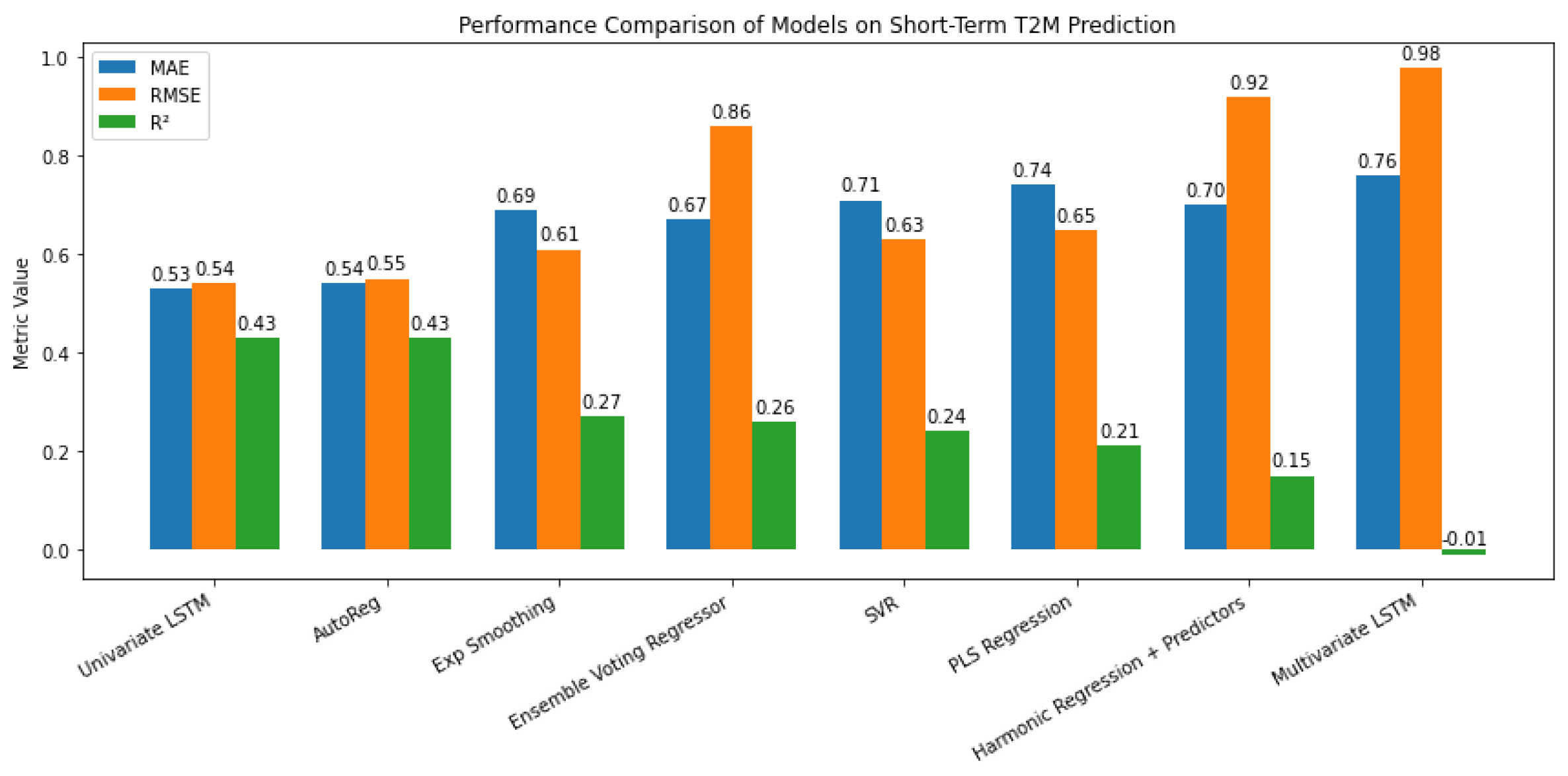
The short-term component captures high-frequency, irregular fluctuations, which are more volatile and less predictable than trend or seasonal patterns [12,13,14]. Figure 12 shows that the Univariate LSTM and AutoReg models performed best (), with low errors, effectively capturing short-term dependencies. Moderate performance was seen for Ensemble Voting Regressor and Exponential Smoothing (), while SVR and PLS Regression had limited predictive power. Harmonic Regression performed poorly (), and Multivariate LSTM underperformed (), suggesting overfitting or difficulty handling multivariate inputs. Default Python settings were used for consistency, though further hyperparameter tuning could improve performance.
Figure 15.
Performance comparison of various models on short-term T2M prediction, showing MAE, RMSE, and R² for each model.
Figure 15.
Performance comparison of various models on short-term T2M prediction, showing MAE, RMSE, and R² for each model.
3.5. Additive Model Analysis
In this section we present an additive framework to represent the surface air temperature series, integrating its short-term variations, seasonal pattern, and long-term trend. Equation 6 presents the mathematical formulation of linear regression; a similar approach can also be applied to Ridge and Lasso regression models, taking into account their respective regularization requirements. Unlike Ridge and Lasso, which extend linear regression through explicit regularization terms, Random Forest and XGBoost do not rely on a single analytical equation; instead, they generate predictions through ensembles of decision trees based on algorithmic rules and hyperparameter tuning.
where represents the raw dependent variable, are the variables of the long-term component, and represent their corresponding coefficients. Likewise, represent the variables of the seasonal-term component, with coefficients , and represent the variables of the short-term component, with corresponding coefficients . The term represents the error term, and t denotes time.
Tree-based ensembles clearly outperform linear methods: XGBoost shows the best performance (MAE = 0.22, RMSE = 0.29, = 0.91), closely followed by Random Forest (MAE = 0.23, RMSE = 0.30, = 0.91) (Figure 16). These results highlight the effectiveness of ensemble models in capturing complex nonlinear relationships. Ridge Regression performs best among linear models, slightly outperforming Lasso and matching Linear Regression, while Random Forest and XGBoost achieve the highest accuracy. Tree-based ensembles excel at capturing complex nonlinear dependencies, whereas Ridge offers a simple and interpretable alternative.
Figure 17 shows that ALLSKY_SFC_SW_DWN has a strong positive seasonal influence, especially in tree-based models (0.63 in Random Forest, 0.55 in XGBoost), while its long- and short-term components are less important. WS2M and RH2M show negative seasonal coefficients in linear models but modest positive importance in ensembles, indicating tree models capture non-linear interactions missed by linear methods. PRECTOTCORR and Logflow contribute moderately and consistently, while Groundwater and GWETROOT exhibit divergent patterns: strong linear coefficients but minimal ensemble importance, suggesting limited non-linear effects. Short-term predictors generally have low linear weights but small consistent importance in tree-based models, highlighting the ensembles’ ability to detect weak or indirect non-linear signals.
Figure 18 summarizes the numerical results, reflecting how each component contributes to the model’s output under different methods. In the top row, the three linear models-Linear Regression, Ridge, and Lasso-show very similar behavior, each achieving a correlation coefficient of 0.93 with the actual values. All three follow the overall wave-like shape of the data quite well but tend to miss some of the sharper turning points. This is especially noticeable during the steep rises and drops, where the predictions either lag slightly or fail to reach the same peaks and troughs as the actual series. Looking at the lower row, on the other hand, the Random Forest and XGBoost models provide a noticeably closer fit to the observed data, with correlation coefficients of 0.95 and 0.96, respectively. Their prediction lines nearly overlap the actual curve throughout the entire period. XGBoost, in particular, captures the full amplitude and direction of variation, even at the extremes, demonstrating superior ability to learn the underlying structure, especially in sections where the signal exhibits rapid shifts or nonlinear changes.
4. Discussion and Conclusion
The results from the walk-forward validation across the three temporal components—long-term, seasonal, and short-term—reveal essential differences in model performance, which can inform the selection of forecasting approaches depending on the nature of the data. Tree-based models—Random Forest and XGBoost in particular—performed better than linear approaches for the long-term component. Their higher values (0.91) and lower RMSE (0.24) and MAE (0.09) imply that they are more appropriate for capturing intricate, non-linear patterns. Lasso Regression performed poorly, perhaps because it oversimplifies the model by aggressively decreasing coefficients, whereas Ridge model and basic Linear Regression, performed moderately. This implies that for long-term forecasting, where interactions may be more complicated, ensemble techniques are preferable.
Among all components, the seasonal term demonstrated superior performance, with Random Forest and XGBoost obtaining near-perfect scores (0.99) and the lowest error rates (RMSE: 0.10–0.11; MAE: 0.05–0.06). This implies that these models are quite effective at recognizing and simulating recurring patterns. Additionally, Ridge and Linear Regressions performed well (: 0.97), suggesting that there may be a sizable linear component to seasonal changes. The slight advantage of tree-based models, however, indicates that there are more non-linearities that linear approaches overlook. Lasso Regression again underperformed, reinforcing its limitations in scenarios requiring nuanced pattern recognition.
The short-term component, on the other hand, proved challenging for all models, with values ranging from 0.19 to 0.23. Although the differences were small, Random Forest had a slight advantage, indicating that short-term fluctuations are extremely unpredictable when using traditional machine learning methods. This is consistent with the hypothesis that short-term noise is stochastic in nature and complex to describe without the use of specialized techniques, such as autoregressive models or more advanced feature engineering.
The application of specialized techniques (Figure 12) yielded improved results, with Univariate LSTM and AutoReg achieving the highest (0.43) and the lowest errors (MAE: 0.53–0.54; RMSE: 0.54–0.55). This demonstrates that time-series-specific methods, particularly those capable of capturing temporal dependencies like LSTMs and autoregressive models, outperform traditional machine learning approaches for short-term forecasting. Exponential Smoothing also showed reasonable performance (: 0.27), though it was less accurate than LSTM and AutoReg. In contrast, more complex methods like Multivariate LSTM performed poorly (: -0.08), likely due to overfitting or the increased difficulty of modeling multiple short-term predictors effectively. These findings imply that, although specialized methods can improve the accuracy of short-term predictions, relatively straightforward univariate time-series models might be more dependable than intricate multivariate methods for this purpose. The findings emphasis how crucial it is to properly select a model based on the particular characteristics of short-term data.
As shown in Figure 3 and Figure 16, the core comparison is between two settings: applying each model directly to the raw time series versus applying the same model to the combined set of decomposed components (long-term, seasonal, and short-term) in an additive framework. In the additive setting, each model receives all three components together as input features to generate a single prediction. The results demonstrate that this approach yields substantial gains across all models. For example, the MAE of Ridge regression dropped from 0.49 on the raw data to 0.29 when trained on the additive components, with RMSE improving from 0.62 to 0.37 and increasing from 0.61 to 0.86. Random Forest and XGBoost saw even greater performance boosts: XGBoost’s RMSE decreased from 0.44 to 0.29, and improved from 0.80 to 0.91. These improvements highlight how supplying the model with explicitly structured temporal features—rather than a single undifferentiated series—enhances its ability to capture underlying patterns.
These results demonstrate how combining ensemble learning and statistical techniques can increase accuracy of time-series reconstruction and forecasting. Such improvements can enhance early-warning systems by providing more reliable trend detection and timely alerts for decision-makers, particularly in climate- or hydrology-sensitive domains. Overall, ensemble models such as Random Forest and XGBoost benefited the most from the additive modeling framework, as the inclusion of decomposed components allowed them to more effectively capture nonlinear patterns and interactions across different temporal scales.
Author Contributions
K.A., D.Z., A.F., K.T., and A.M. contributed to the conceptualization, methodology, software application to the data, formal analysis, visualization of results, and writing, review, and editing of different parts of the manuscript.
Funding
This research received no external funding.
Acknowledgments
The authors would like to acknowledge the anonymous reviewers for their careful reading of the manuscript.
Conflicts of Interest
The authors declare no conflict of interest.
References
- Wu, L.X.; An, J.L.; Jin, D. Predictive model for o3 in shanghai based on the kz filtering technique and lstm. Huan jing ke xue= Huanjing kexue 2024, 45, 5729–5739. [Google Scholar] [PubMed]
- Kumar, V.; Sur, S.; Senarathna, D.; Gurajala, S.; Dhaniyala, S.; Mondal, S. Quantifying impact of correlated predictors on low-cost sensor pm2.5 data using kz filter. Frontiers in Applied Mathematics and Statistics 2024, 10. [Google Scholar] [CrossRef]
- Nafarrate, A.; Petisco-Ferrero, S.; Idoeta, R.; Herranz, M.; Sáenz, J.; Ulazia, A.; Ibarra-Berastegui, G. Applying the kolmogorov–zurbenko filter followed by random forest models to 7be observations in spain (2006–2021). Heliyon 2024, 10. [Google Scholar] [CrossRef] [PubMed]
- Agbehadji, I.E.; Obagbuwa, I.C. Systematic review of machine learning and deep learning techniques for spatiotemporal air quality prediction, 2024. [CrossRef]
- Wu, L.; An, J. Quantitative impacts of meteorology and emissions on the long-term trend of o3 in the yangtze river delta (yrd), china from 2015 to 2022. Journal of Environmental Sciences 2025, 149, 314–329. [Google Scholar] [CrossRef] [PubMed]
- Yao, T.; Ye, H.; Wang, Y.; Zhang, J.; Guo, J.; Li, J. Kolmogorov-zurbenko filter coupled with machine learning to reveal multiple drivers of surface ozone pollution in china from 2015 to 2022. Science of The Total Environment 2024, 949, 175093. [Google Scholar] [CrossRef] [PubMed]
- Fang, C.; Qiu, J.; Li, J.; Wang, J. Analysis of the meteorological impact on pm2.5 pollution in changchun based on kz filter and wrf-cmaq. Atmospheric Environment 2022, 271, 118924. [Google Scholar] [CrossRef]
- Valachovic, E. An extension of the iterated moving average. Technical report.
- Mahmood, K.K. Statistical analysis for decomposed multivariate time series data with an application to water discharge forecasting. Phd thesis, University of Brighton, UK, 2019.
- Tsakiri, K.G.; Zurbenko, I.G. Prediction of ozone concentrations using atmospheric variables. Air Quality, Atmosphere & Health 2011, 4, 111–120. [Google Scholar] [CrossRef]
- Tsakiri, K.; Marsellos, A.; Kapetanakis, S. Artificial neural network and multiple linear regression for flood prediction in mohawk river, new york. Water (Switzerland) 2018, 10. [Google Scholar] [CrossRef]
- Hyndman, R.J.; Athanasopoulos, G. Forecasting: Principles and Practice; OTexts: Melbourne, Australia, 2018. [Google Scholar]
- Chatfield, C.; Xing, H. The Analysis of Time Series: An Introduction with R; Chapman and Hall/CRC: Boca Raton, FL, USA, 2019. [Google Scholar]
- Shumway, R.H.; Stoffer, D.S. Time series analysis and its applications: with r examples; Springer, 2006.
Figure 1.
Geographic locations of the data sources used in the study: NASA/POWER grid point, USGS streamflow gauge at Keosauqua (Site 05490500), and USGS groundwater well in Jefferson County (Site 405451091483301).
Figure 1.
Geographic locations of the data sources used in the study: NASA/POWER grid point, USGS streamflow gauge at Keosauqua (Site 05490500), and USGS groundwater well in Jefferson County (Site 405451091483301).
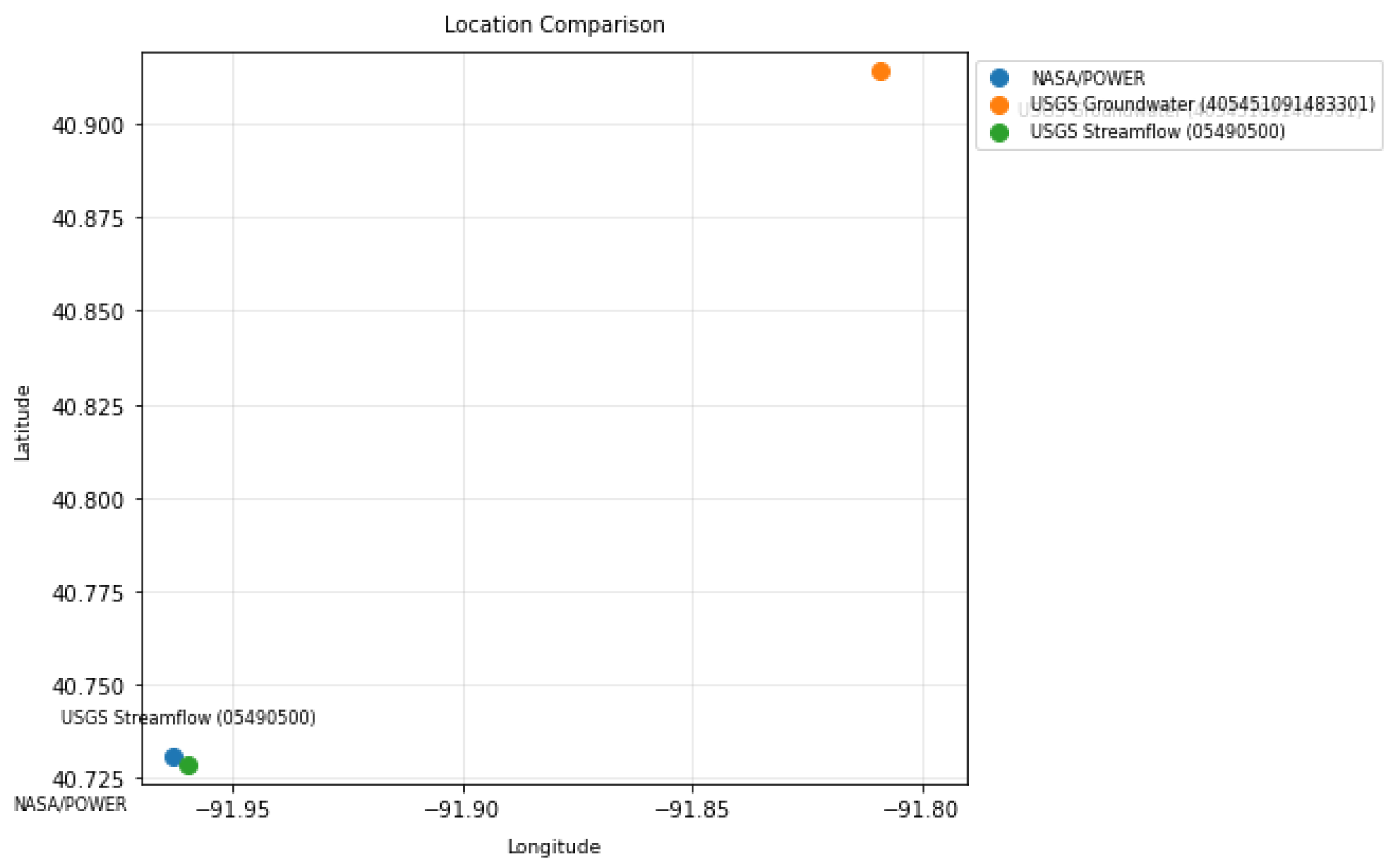
Figure 2.
KZ decomposition of the T2M time series using parameters and , separating the data into long-term, seasonal, and short-term components.
Figure 2.
KZ decomposition of the T2M time series using parameters and , separating the data into long-term, seasonal, and short-term components.
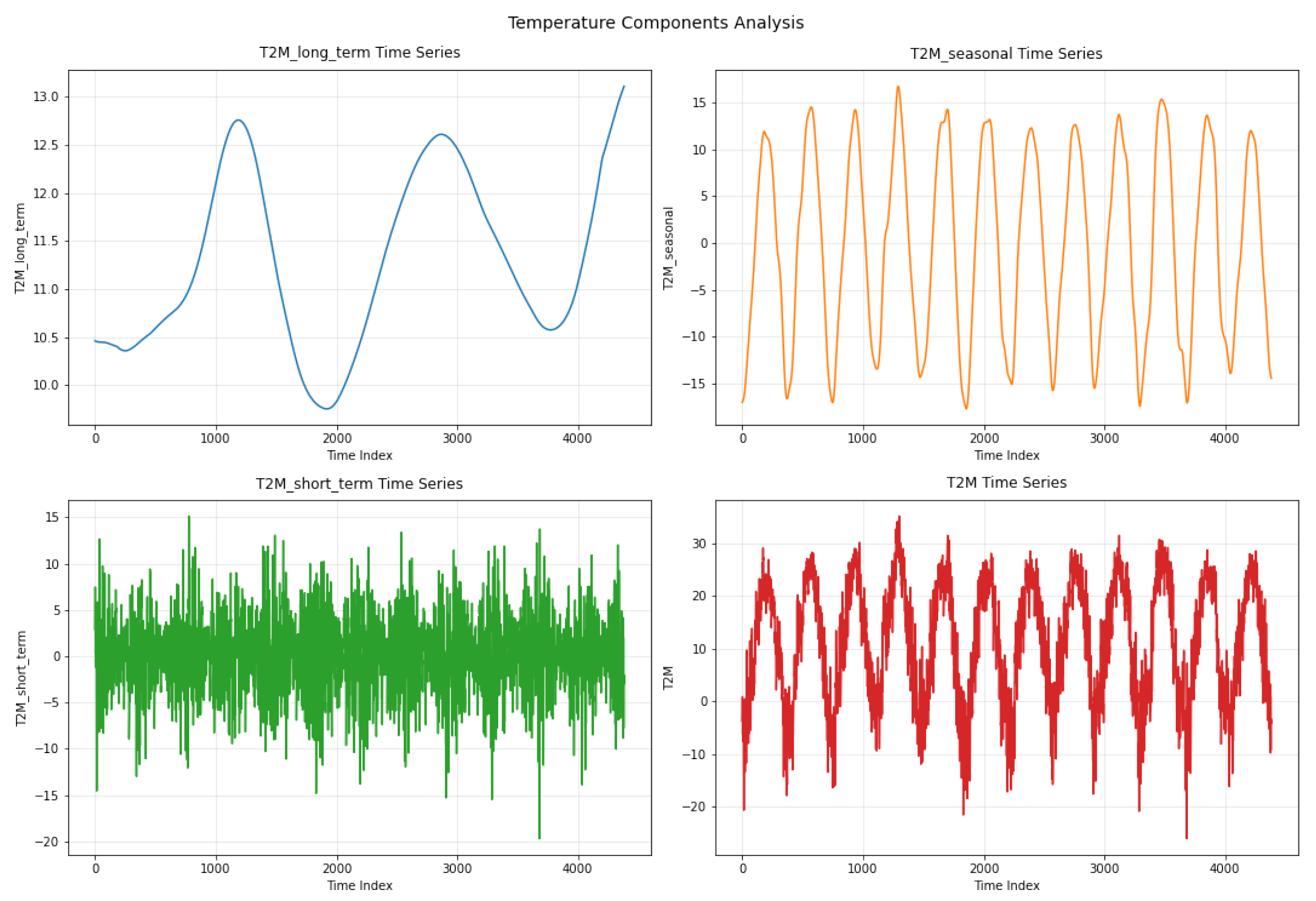
Figure 3.
Walk-forward validation metrics (MAE, RMSE, R²) for five regression models for the raw data, showing improved performance of Random Forest and XGBoost compared to linear models.
Figure 3.
Walk-forward validation metrics (MAE, RMSE, R²) for five regression models for the raw data, showing improved performance of Random Forest and XGBoost compared to linear models.
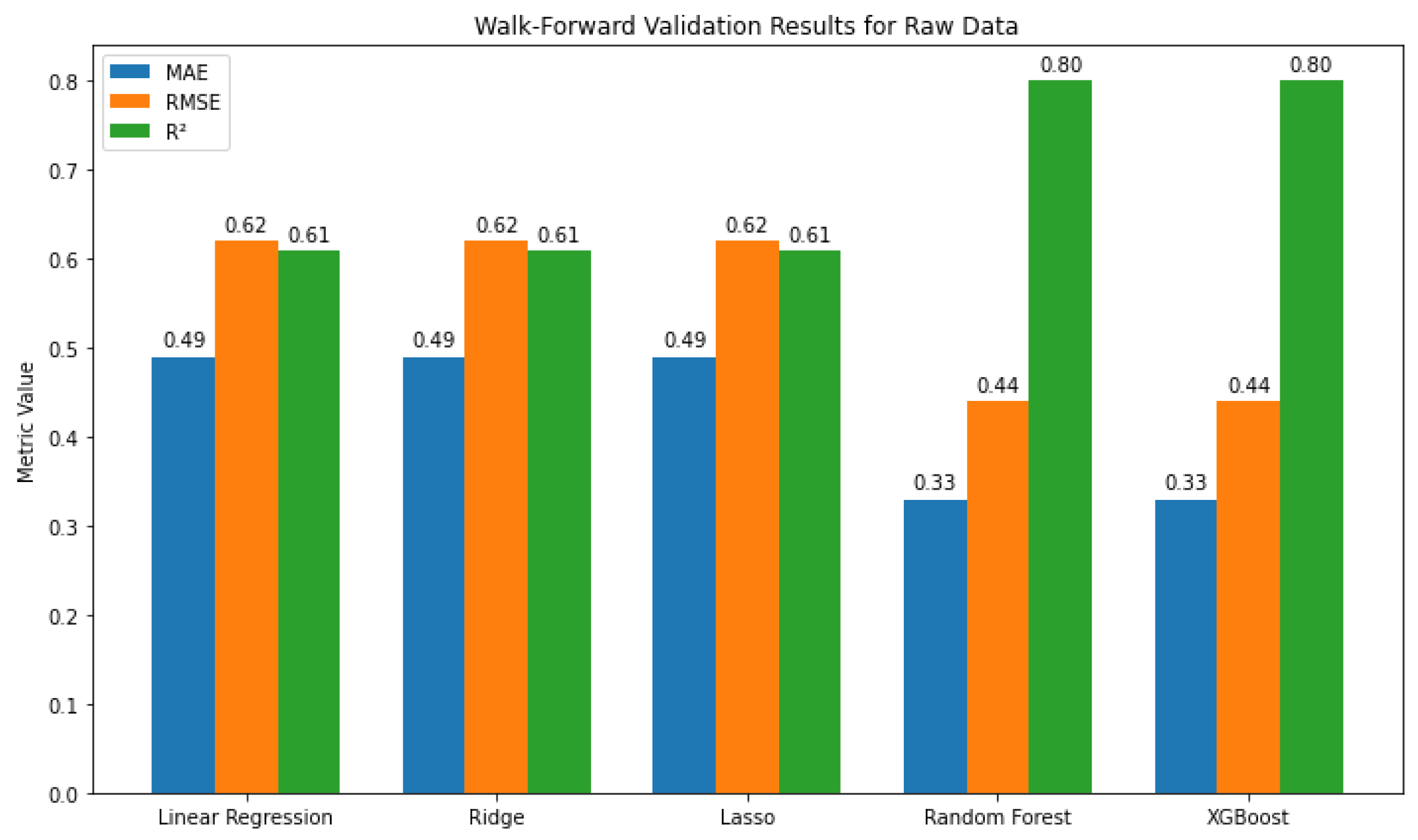
Figure 4.
Predictor importance across models, highlighting solar radiation as dominant, GWETROOT as most negative, and minimal impact of WS2M.
Figure 4.
Predictor importance across models, highlighting solar radiation as dominant, GWETROOT as most negative, and minimal impact of WS2M.
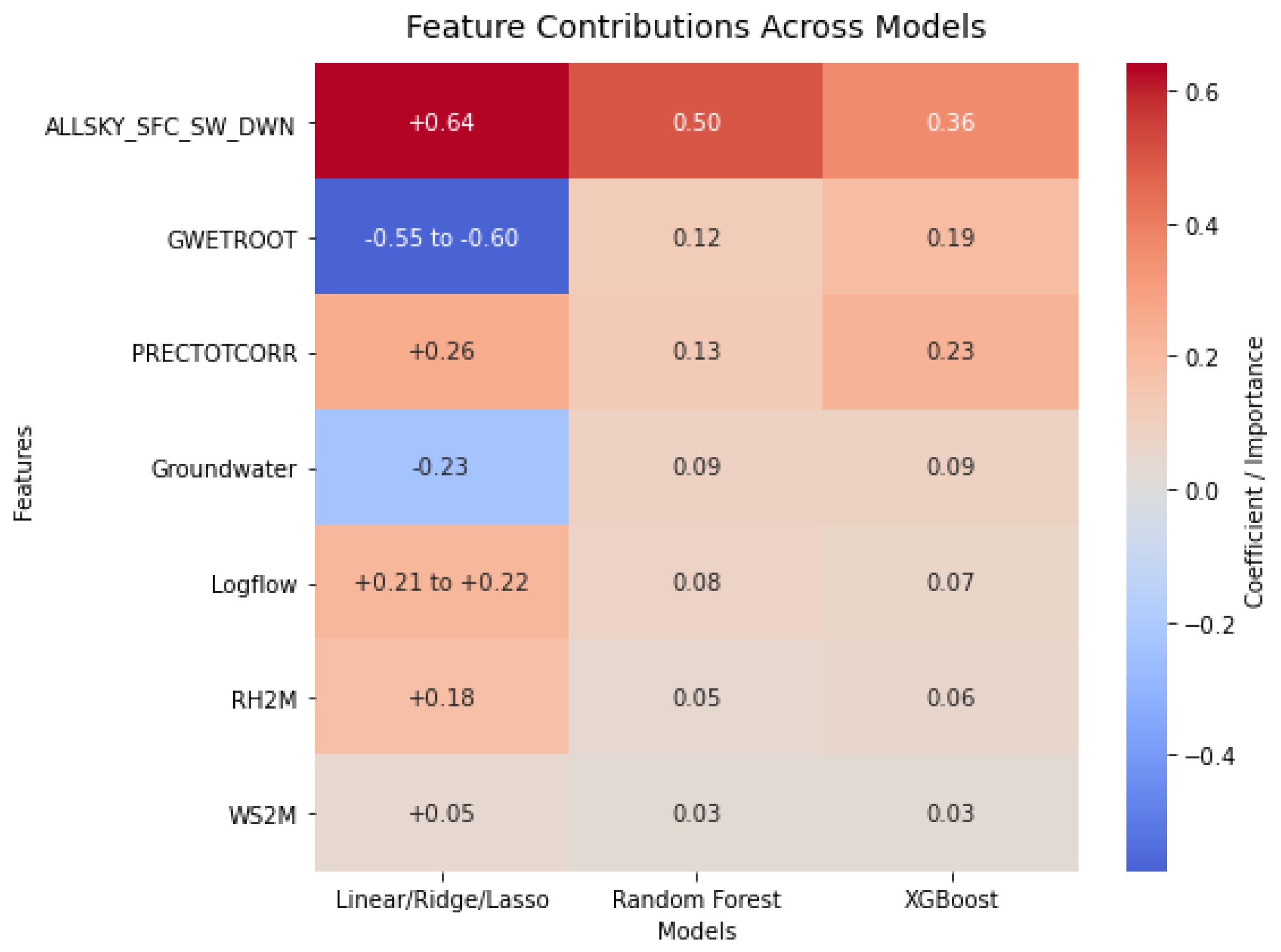
Figure 5.
Time series of actual values versus model predictions with Pearson correlation coefficients () for the raw data.
Figure 5.
Time series of actual values versus model predictions with Pearson correlation coefficients () for the raw data.
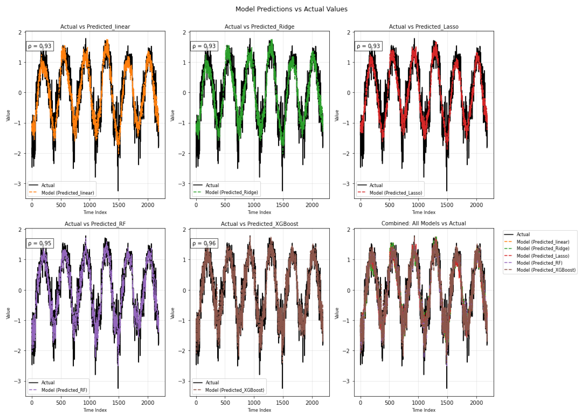
Figure 6.
Walk-forward validation metrics (MAE, RMSE, R²) for the long-term component across five models, highlighting superior performance of Random Forest and XGBoost.
Figure 6.
Walk-forward validation metrics (MAE, RMSE, R²) for the long-term component across five models, highlighting superior performance of Random Forest and XGBoost.
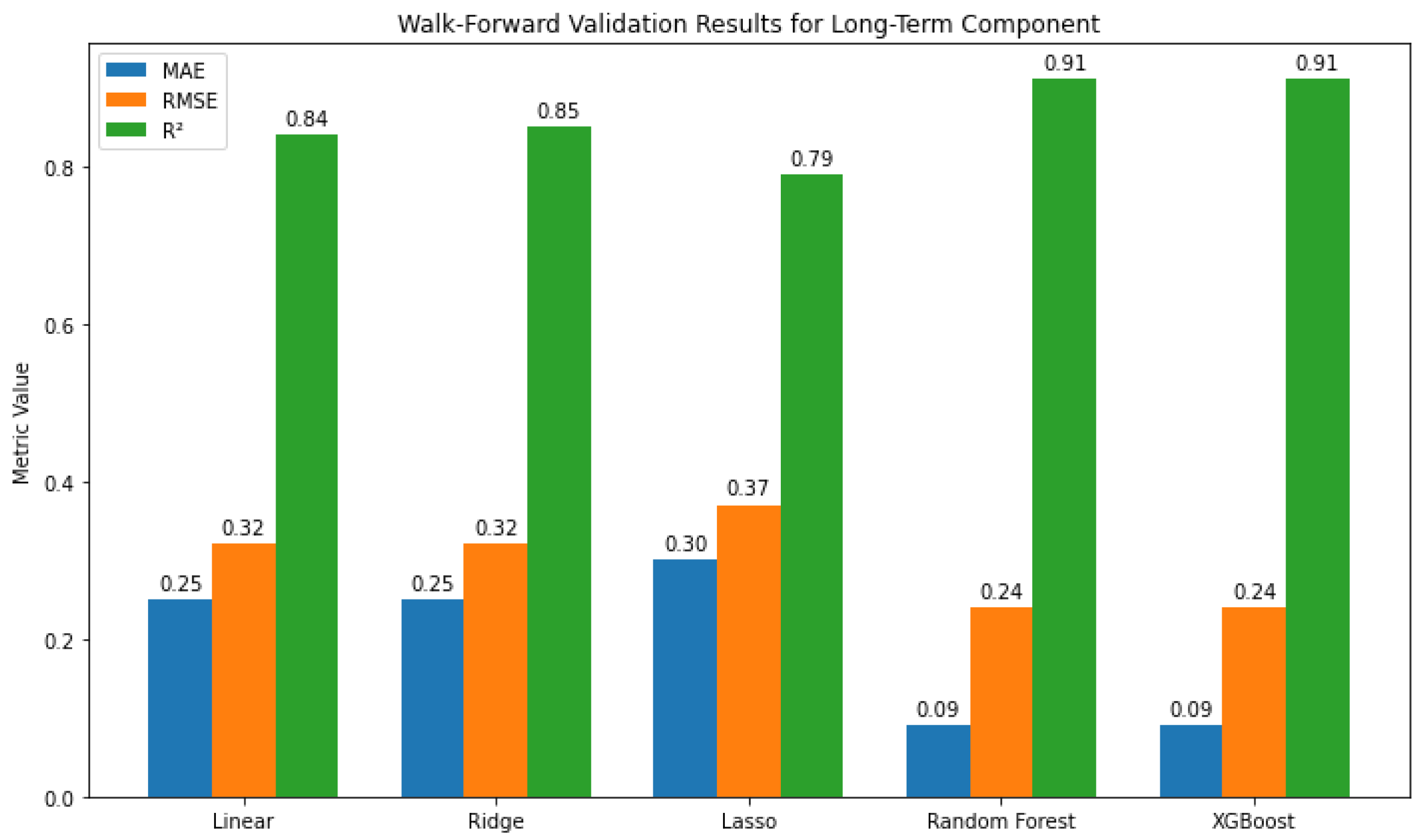
Figure 7.
Heatmap of long-term predictor contributions across models, showing ALLSKY_SFC_SW_DWN and GWETROOT as the strongest positive drivers, while PRECTOTCORR and RH2M exert negative effects.
Figure 7.
Heatmap of long-term predictor contributions across models, showing ALLSKY_SFC_SW_DWN and GWETROOT as the strongest positive drivers, while PRECTOTCORR and RH2M exert negative effects.
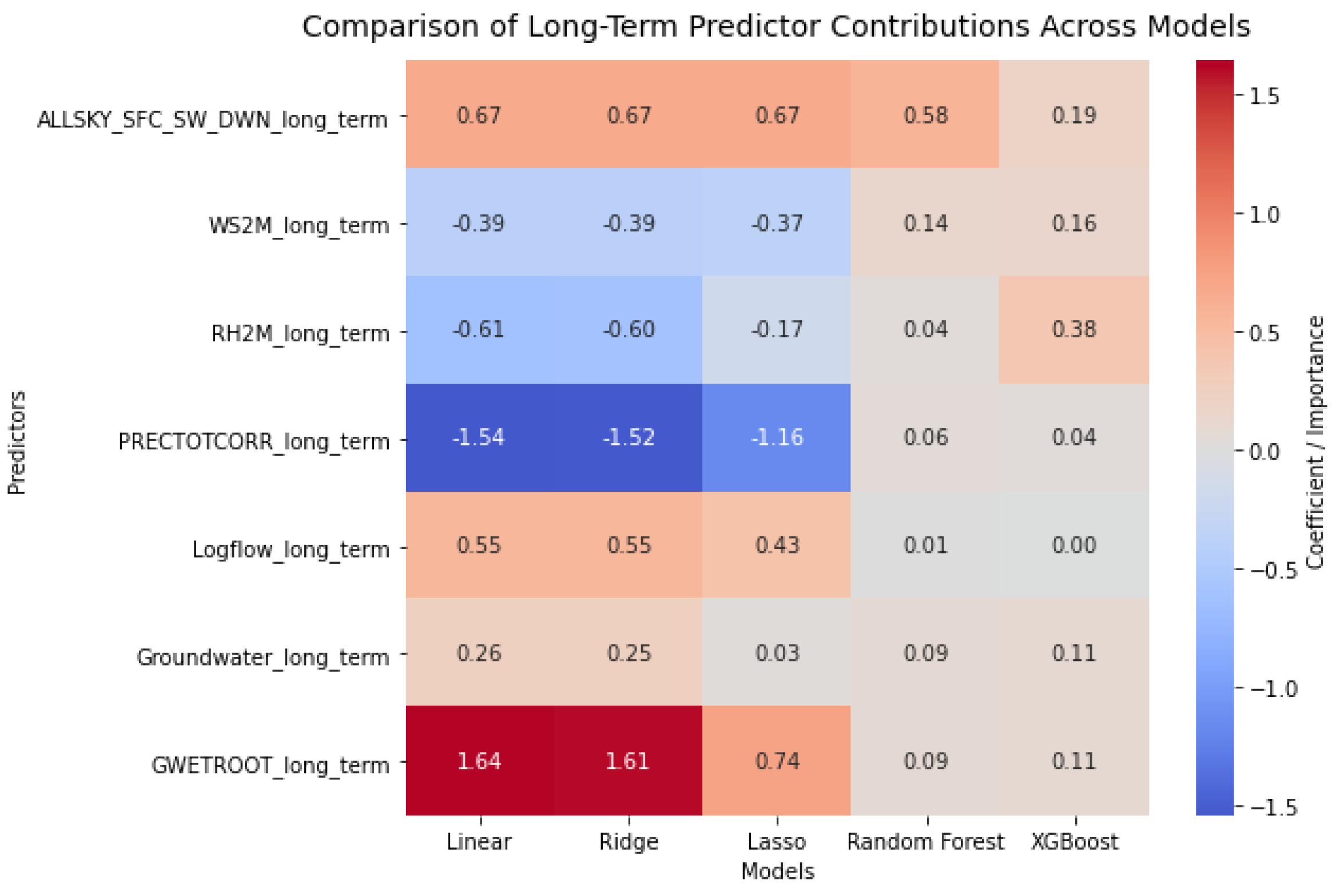
Figure 8.
Time series of actual values versus model predictions with Pearson correlation coefficients () for the long-term.
Figure 8.
Time series of actual values versus model predictions with Pearson correlation coefficients () for the long-term.
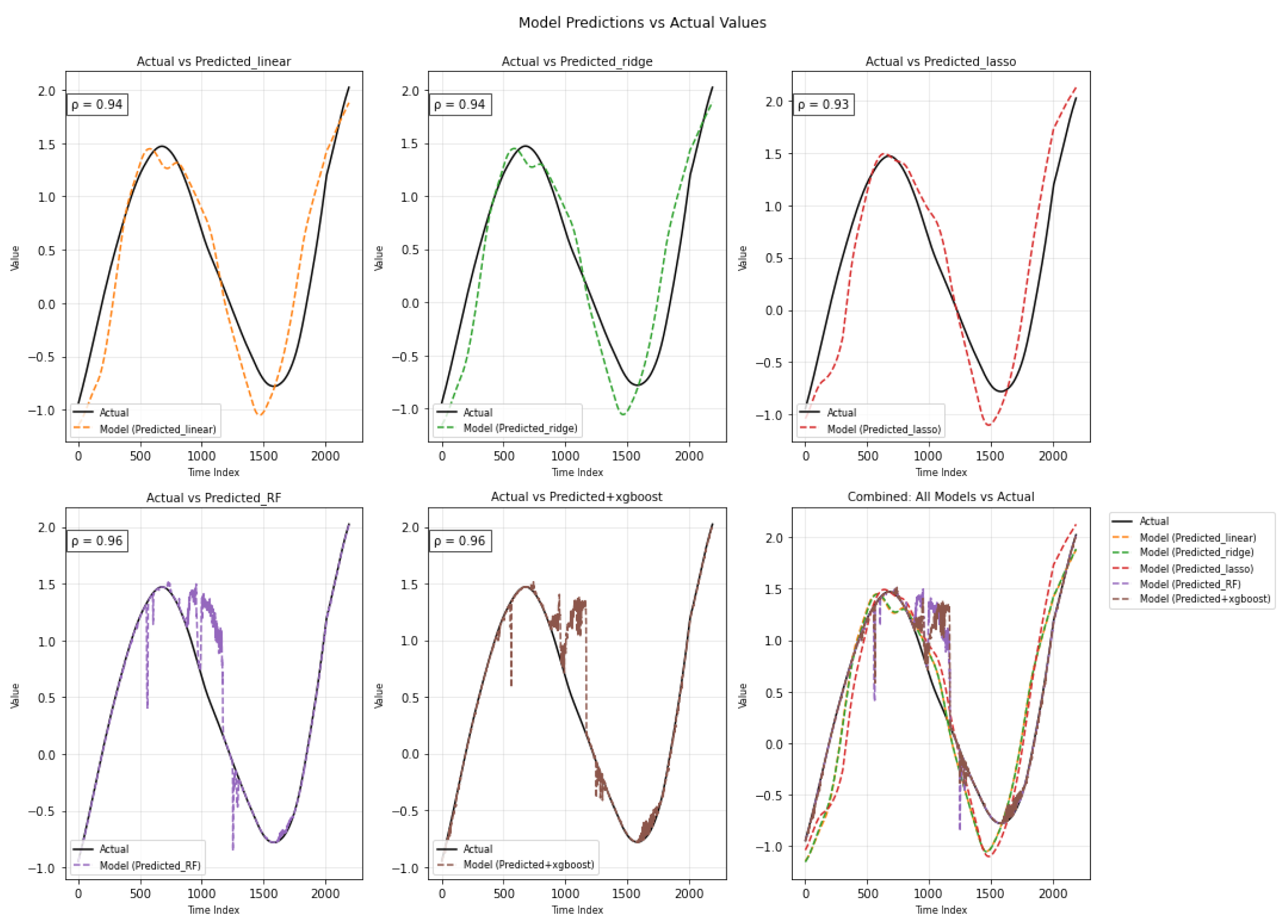
Figure 9.
Walk-forward validation metrics (MAE, RMSE, R²) for the seasonal component, showing strong performance of Random Forest and XGBoost compared to linear models.
Figure 9.
Walk-forward validation metrics (MAE, RMSE, R²) for the seasonal component, showing strong performance of Random Forest and XGBoost compared to linear models.
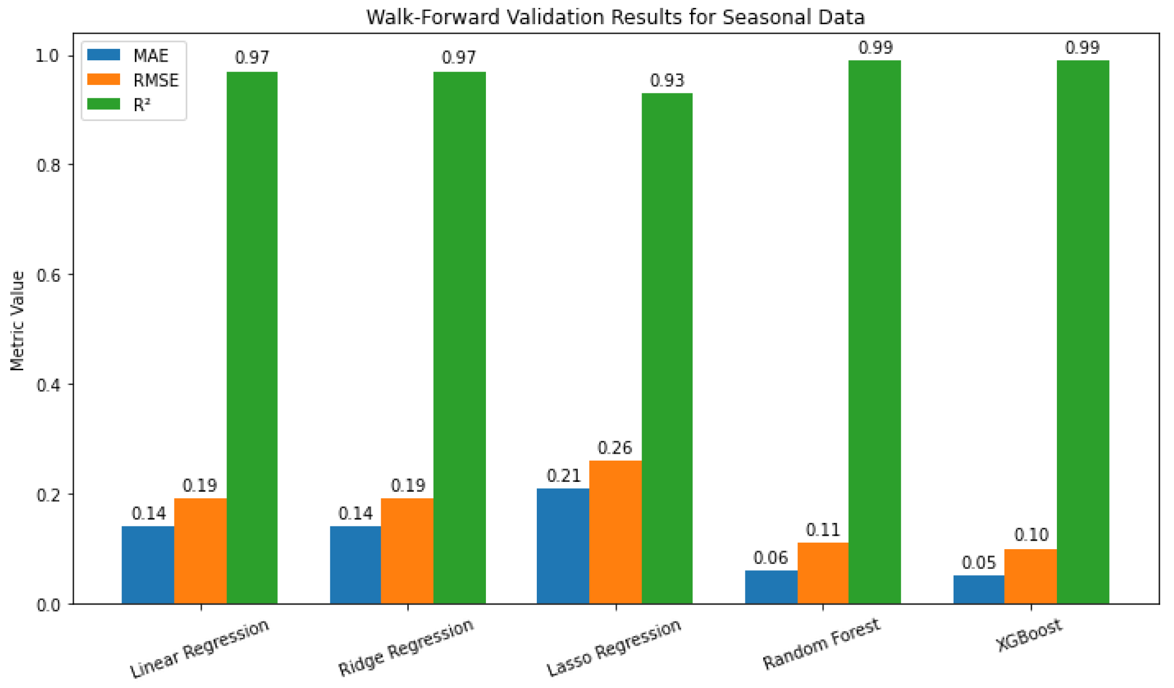
Figure 10.
Walk-forward cross-validation results for T2M_seasonal_term.
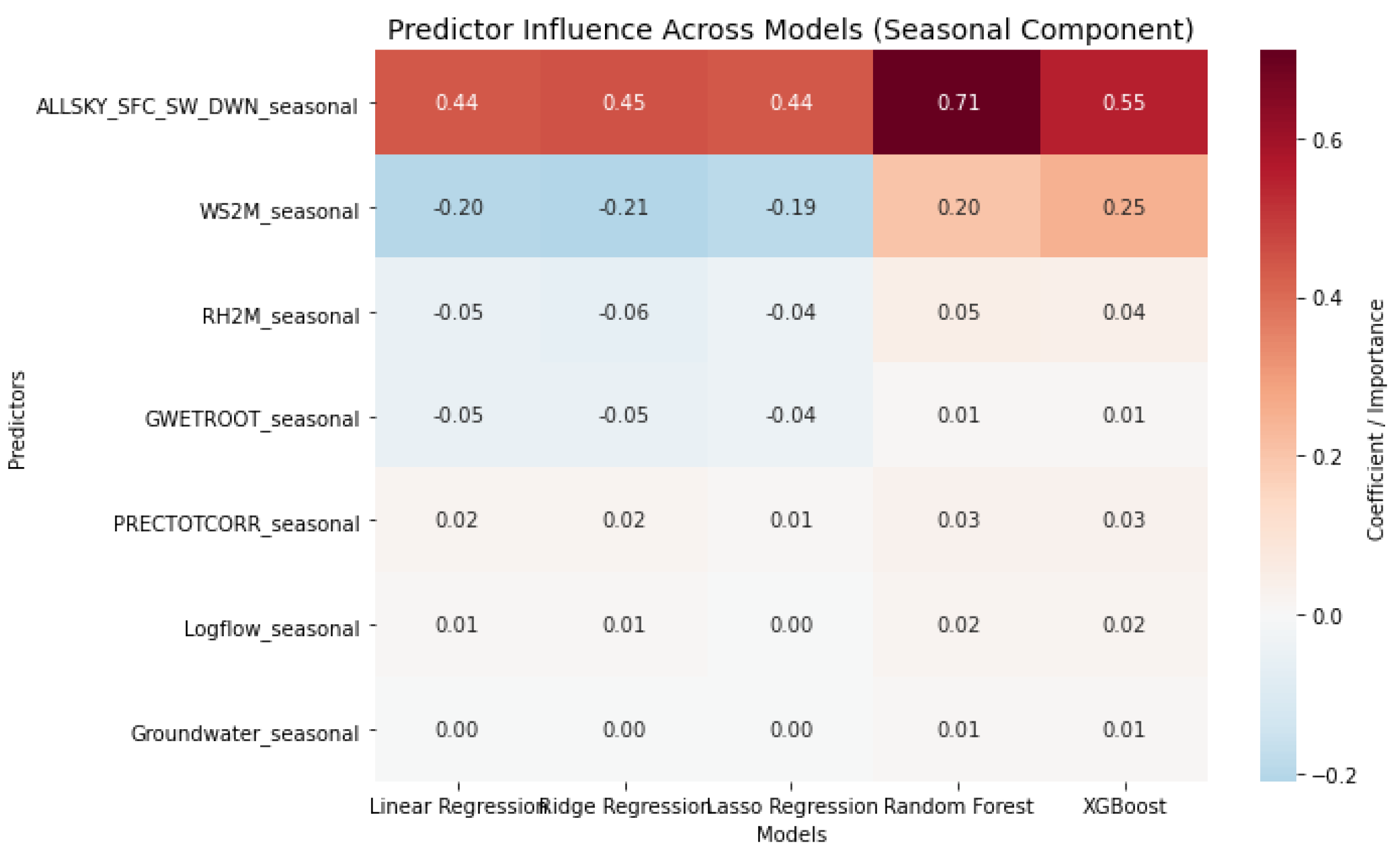
Figure 11.
Time series of actual values versus model predictions with Pearson correlation coefficients () for seasonal variations
Figure 11.
Time series of actual values versus model predictions with Pearson correlation coefficients () for seasonal variations
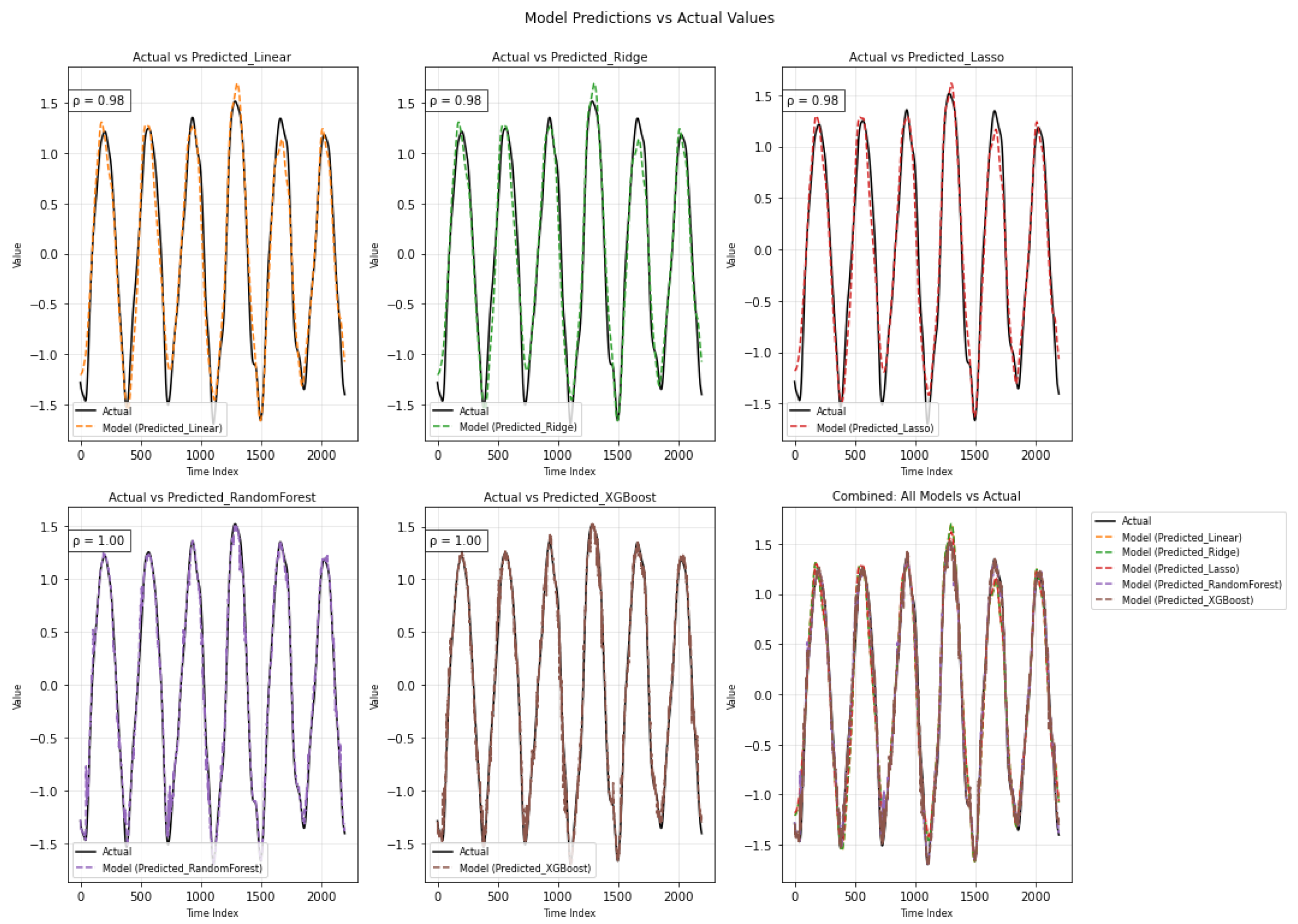
Figure 12.
Walk-Forward Validation results for short-term data showing the performance of five models in terms of MAE, RMSE, and .
Figure 12.
Walk-Forward Validation results for short-term data showing the performance of five models in terms of MAE, RMSE, and .
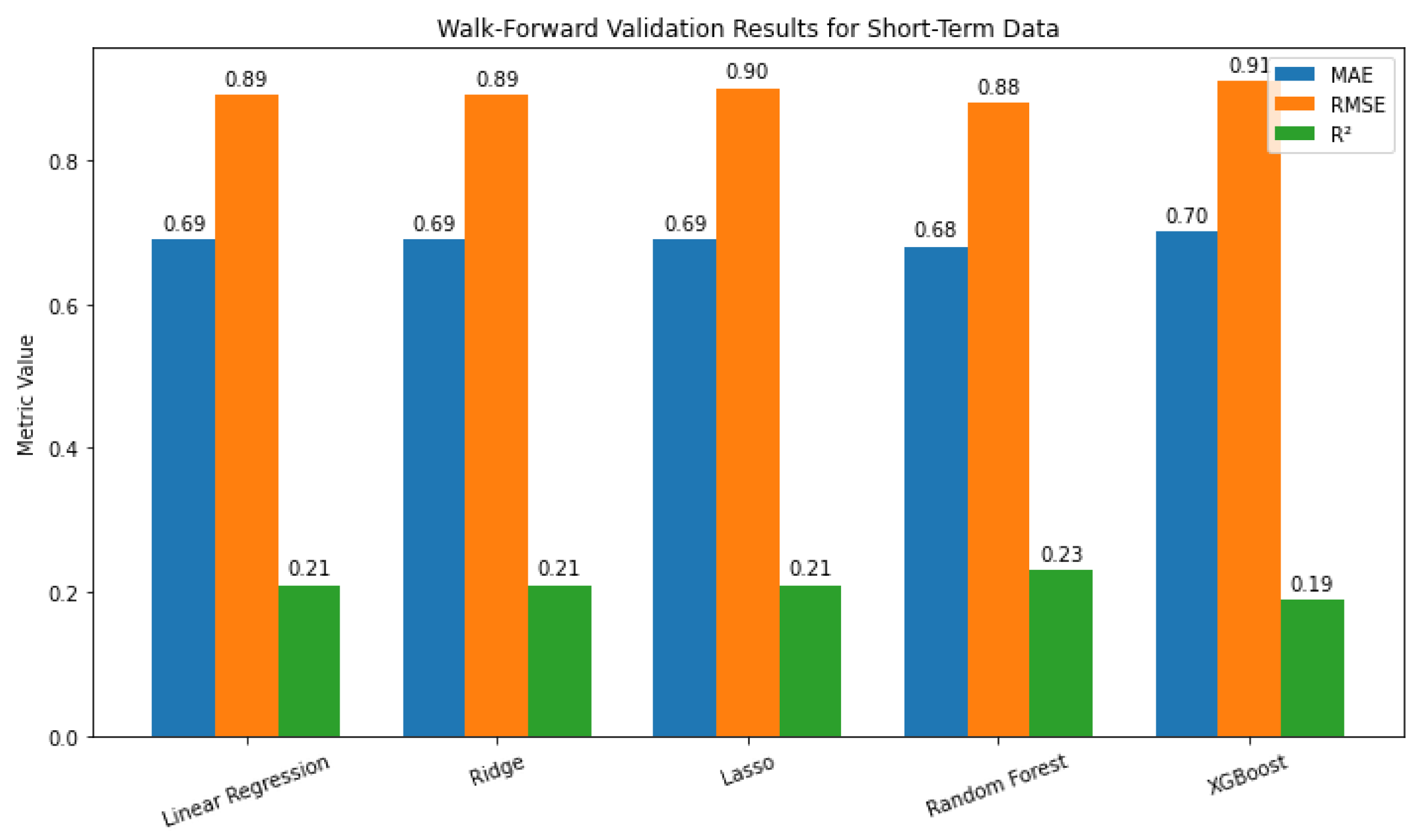
Figure 13.
Walk-forward cross-validation results for T2M short-term.
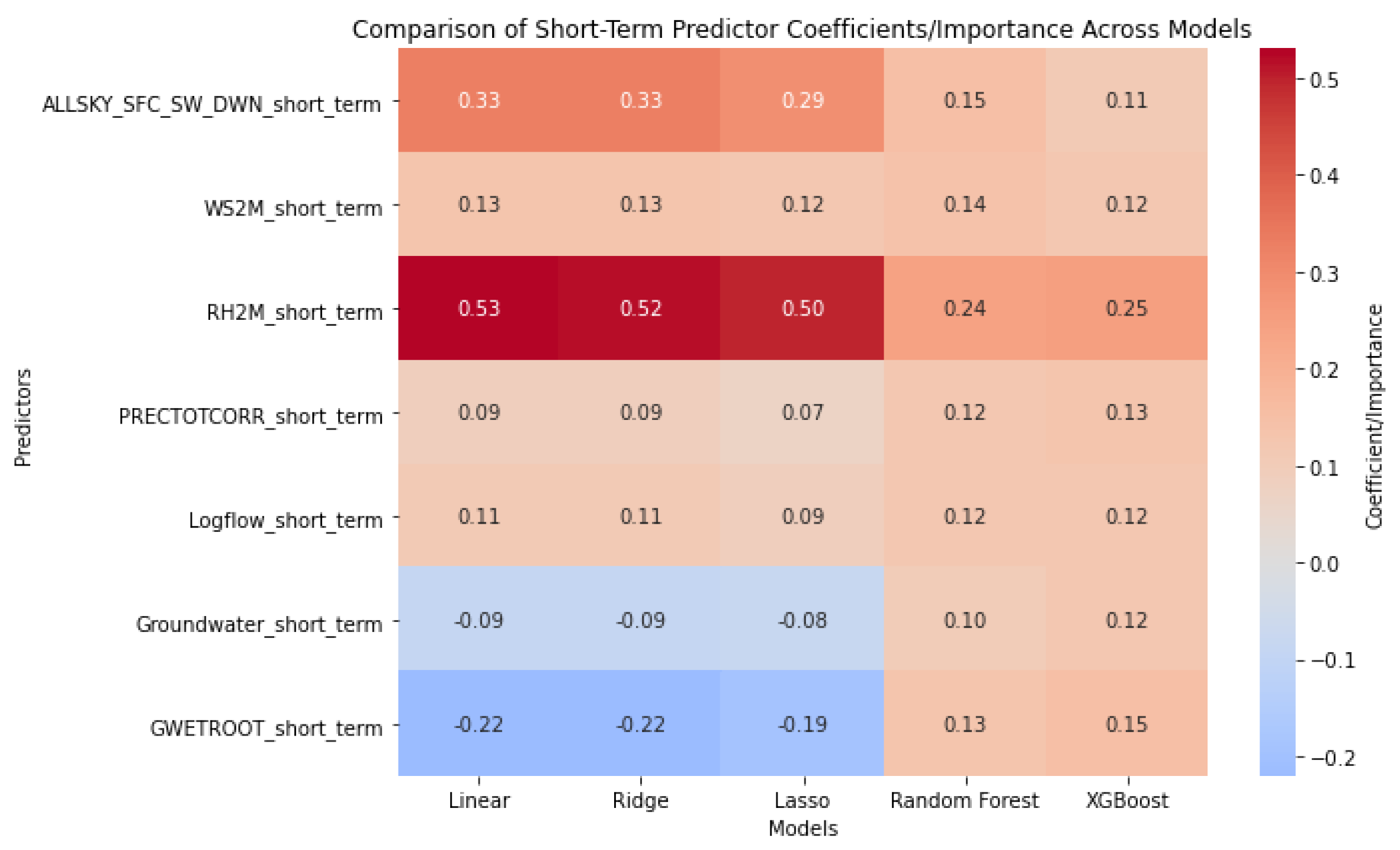
Figure 14.
Time series of actual values versus model predictions for short term.
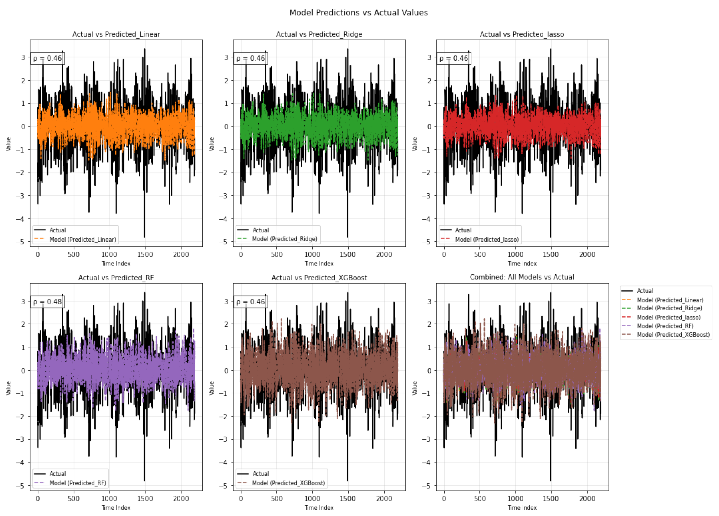
Figure 16.
Performance comparison of various models on additive, showing MAE, RMSE, and R² for each model.
Figure 16.
Performance comparison of various models on additive, showing MAE, RMSE, and R² for each model.
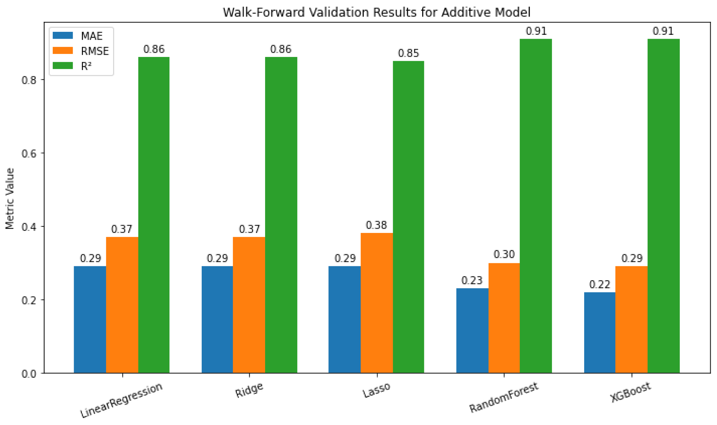
Figure 17.
Walk-forward cross-validation results for additive model.
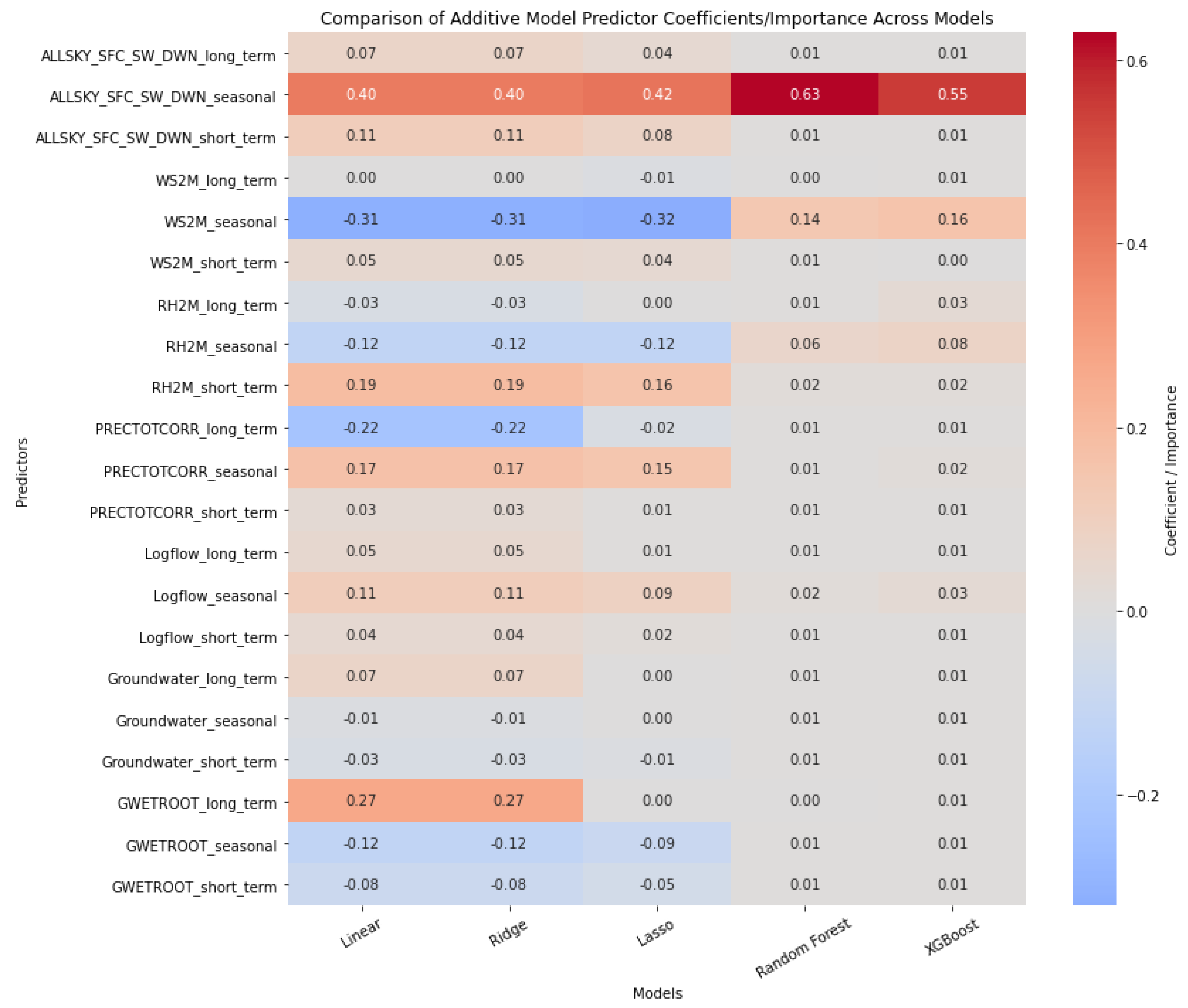
Figure 18.
Time series of actual values versus model predictions for additive models.
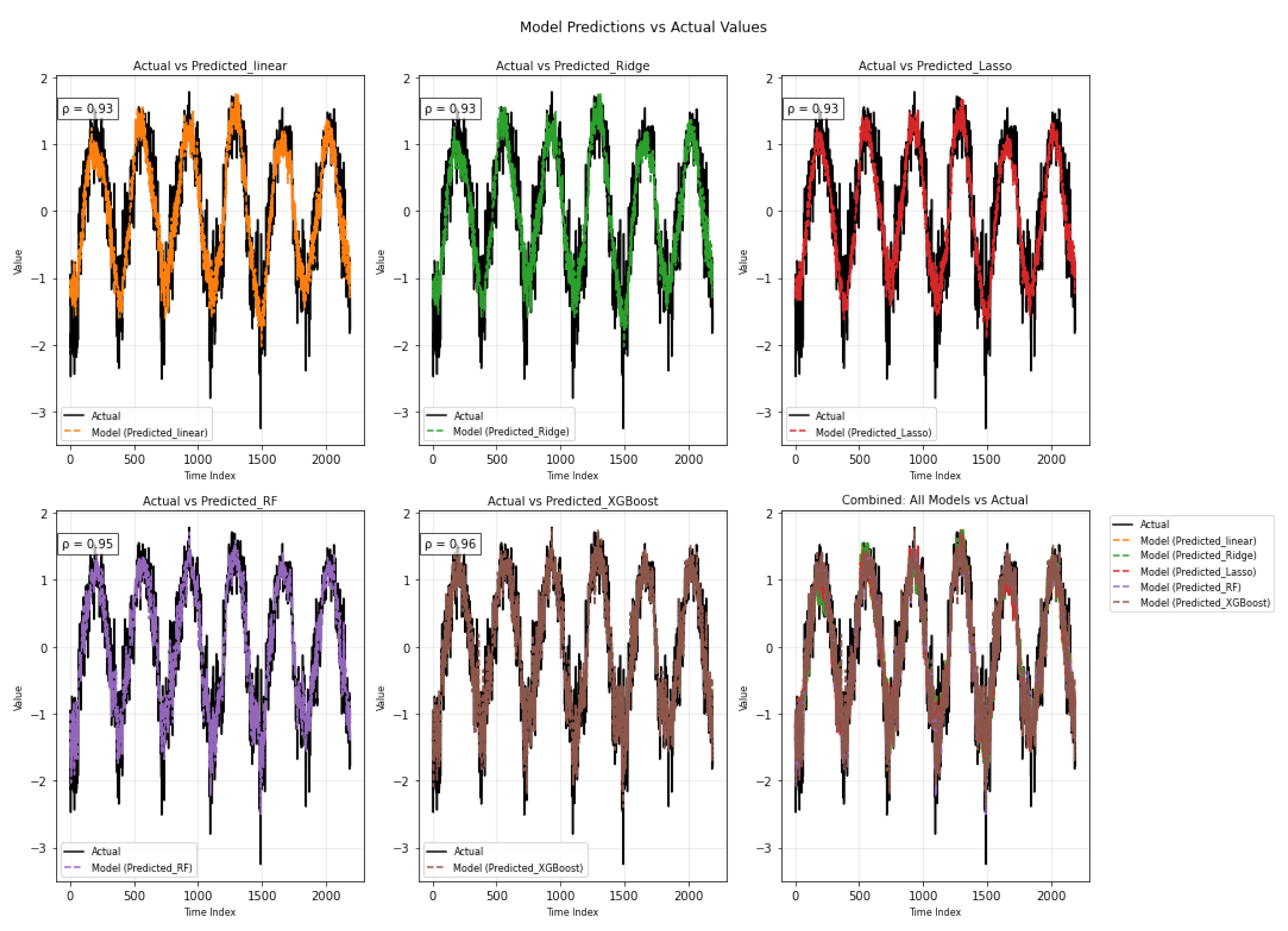

Table 1.
Meteorological and environmental variables used in this study.
| Variable (Abbreviation) | NASA/Source Name | Description | Unit |
|---|---|---|---|
| ALLSKY SFC SW DWN | CERES SYN1deg All Sky Surface Shortwave Downward Irradiance | Incoming solar radiation at the surface under all-sky conditions | W/m² |
| GWETROOT | MERRA-2 Root Zone Soil Wetness | Soil moisture content in the top 1 m of soil | Fraction (0–1) |
| WS2M | NASA/POWER Wind Speed at 2 Meters | Horizontal wind speed at 2 m above ground | m/s |
| RH2M | NASA/POWER Relative Humidity at 2 Meters | Relative humidity at 2 m height | % |
| T2M | NASA/POWER Temperature at 2 Meters | Air temperature at 2 m above surface | °C |
Table 2.
Hydrological variables obtained from USGS.
| Variable (Abbreviation) | USGS Source | Description | Unit |
|---|---|---|---|
| Logflow | Des Moines River gauge near Keosauqua (Site No. 05490500) | Daily streamflow at the river gauge, log-transformed | m³/s (log) |
| Groundwater Level | Monitoring well in Jefferson County (Site No. 405451091483301) | Daily groundwater level in the monitoring well | m |
Disclaimer/Publisher’s Note: The statements, opinions and data contained in all publications are solely those of the individual author(s) and contributor(s) and not of MDPI and/or the editor(s). MDPI and/or the editor(s) disclaim responsibility for any injury to people or property resulting from any ideas, methods, instructions or products referred to in the content. |
© 2025 by the authors. Licensee MDPI, Basel, Switzerland. This article is an open access article distributed under the terms and conditions of the Creative Commons Attribution (CC BY) license (http://creativecommons.org/licenses/by/4.0/).
Copyright: This open access article is published under a Creative Commons CC BY 4.0 license, which permit the free download, distribution, and reuse, provided that the author and preprint are cited in any reuse.


