Submitted:
17 September 2025
Posted:
19 September 2025
You are already at the latest version
Abstract
This article focuses on the problem of building a real-world predictive maintenance system for hydraulic piston pumps. Particular attention is given to the issue of limited data availability regarding the failure state of systems with a damaged valve plate.
The main objective of this work was to analyze the impact of imbalanced data on the quality of the failure prediction system. Several data balancing techniques, including oversampling, undersampling, and combined methods, were evaluated to overcome the limitations. The dataset used for evaluation includes recordings from eleven sensors, such as pressure, flow, and temperature, registered at various points in the hydraulic system. It also includes data from three additional vibration sensors.
The experiments were conducted with imbalance ratios ranging from 0.5% to a fully balanced dataset. The results indicate that two methods, Borderline SMOTE, SMOTE+Tomek-Links dominate. These methods allowed the system to achieve the highest performance on a completely new dataset with different levels of damaged valve plates, for the balance rate larger than three percent. Furthermore, for balance rates below one percent, the use of data balancing methods may harm the model. Finally, our results indicate the limitations of the use of cross-validation procedure when assessing data balancing methods.
Keywords:
failure prediction
; piston pump
; imbalanced learning
; predictive maintenance
; machine learning
1. Introduction
In recent years, the integration of artificial intelligence and machine learning into industrial operations has revolutionized how companies manage their assets. A primary focus of this transformation is predictive maintenance, a strategy that utilizes advanced analytics to detect impending component failures by continuously monitoring operational data [1]. The ability to forecast equipment issues before they occur is critical for minimizing downtime and maximizing productivity.
The industrial landscape is heavily dependent on the performance and reliability of hydraulic systems, which are foundational to heavy machinery in sectors such as metal processing, construction, and mining. The failure of a hydraulic component, such as a piston pump, can severely compromise the stability of a production process. The economic impact of such events often far outweighs the cost of the component itself. A notable example is the failure of a pump in a coal mine’s long-wall shearer, where a component worth hundreds of euros led to an estimated economic loss in the range of hundreds of thousands of euros.
One of the causes of failure is, for example, contamination of the working fluid (oil). This is often due to improper maintenance (lack of or delayed filter replacement) or improper filling of oil tanks (oil not at the required purity level, errors in start-up procedures, etc.). Another factor accelerating wear or failure is the fact that many hydraulic systems are still built without sensors monitoring oil temperature. As a result, it overheats. This has numerous side effects. First, at elevated temperatures, the kinematic viscosity of the oil becomes approximately two times lower compared to its nominal viscosity. For ISO VG 46 oil, whose nominal viscosity at 40 °C is 46 cSt, at 60 °C, its kinematic viscosity is approximately 20 cSt. As a result, in heavily loaded systems, this can lead to the degrading phenomenon of cavitation in pump components.
This stark imbalance between component cost and failure cost powerfully demonstrates the immense value of accurate predictive failure models.
One of the main challenges in the large-scale implementation of machine learning methods in industry is the availability of training data that adequately describes both normal operational states and failure states. While collecting data from an operational system in a normal state is generally straightforward, obtaining data from failure states is rarely accessible and uncommon. This asymmetry in the class distribution makes the training process difficult, as the training data is highly imbalanced with a dominating normal state and only a few available samples for the minority class, the failure state. Such an unbalanced distribution makes machine learning models difficult to train and prone to incorrect classification. In this work, we evaluate various methods to overcome these difficulties in building an accurate model for recognizing valve plate failures in a piston pump.
This work is a continuation of our previous research presented in [2], which serves as a foundation. In our prior study, we evaluated several prediction methods and analyzed flow, temperature, and pressure sensors required to achieve high prediction accuracy. However, our previous research addressed a balanced classification problem, which is not representative of real-world pump operating conditions. Therefore, this work focuses on analyzing how much failure data is needed to achieve a desired prediction accuracy and how various preprocessing methods aimed at overcoming imbalanced classification influence prediction performance. This study is thus aimed at answering the following research questions:
- How does the amount of failure data influence prediction performance?
- Which preprocessing method is most suitable for dealing with unbalanced classification in the context of valve plate failure prediction?
- What are the limitations of the use of data balancing methods?
- How do oversampling strategies influence predictions by analyzing the changes in feature importance for different methods?
All analyses are conducted on data collected under laboratory conditions for a piston pump. Four states were simulated: one normal state and three failure states with different levels of valve plate degradation. In addition to classical sensors for pressure, temperature, and flow, the collected data includes basic vibration sensor data, such as vibration speed (in accordance with the ISO 20816-3 standard).
The remainder of the manuscript is organized as follows. First, we present the current state of the art in piston pump failure prediction and in dealing with imbalanced data. Section 3 then describes the experimental setup, including the data collection procedure, the machine learning pipeline, and the metrics used. Finally, in Section 4, the obtained results are presented and discussed. The last section, Section 5, summarizes our findings and outlines future research directions.
2. Related Work
This research addresses two independent aspects: the problem of piston pump predictive maintenance and the issue of imbalanced classification. Each of these topics is considered separately below, with a focus on recent progress in each respective field.
2.1. Machine Learning in Pump Failures Prediction
Machine learning techniques are still developing in many fields, including predicting failures in power hydraulic devices. In addition to classic classification methods such as KNN and decision trees, simple and deep neural networks are also used.
The literature compares classic machine learning algorithms, including SVM, KNN, and gradient boosted trees [3].
Nevertheless many authors have emphasized artificial neural networks (ANNs), multilayer perceptrons (MLPs), or convolutional neural networks (CNNs). Article [4] describes an example of using a neural network, particularly a convolutional neural network. Another approach, also based on the use of a convolutional neural network is described in [5,6]. In the presented research, pressure, vibration, and acoustic signals are used as input data for prediction. In [7], the researchers describe a deep learning method that uses a Bayesian optimization (BO) algorithm to find the best model hyperparameters. In this paper, the vibration signal of a piston pump is used as a data source. CWT preprocesses the signal, and then a preliminary CNN model is prepared. Finally, a Gaussian-based BO was used to prepare an adaptive CNN model (CNN-BO).Another solution, based on the use of RBF neural networks combined with noise filtering algorithms and vibration diagnostics, is presented in [8].
However, we see that classic machine learning algorithms are dominating techniques in this area. Examples of using a modified KNN algorithm, combined with the just-in-time learning (JITL) principle, can be found to determine the remaining useful life (RUL) [9]. This method was applied to hydraulic pumps, taking into account pressure measurements. The authors of [8,10] also use the term RUL in conjunction with a Bayesian regularized radial basis function neural network (Trainbr-RBFNN) when studying an external gear pump, or modified auto-associative kernel regression (MAAKR) and monotonicity-constrained particle filtering (MCPF) while working with a piston pump. Remaining useful life is also studied in [11], using the autoregressive integrated moving average (ARIMA) forecasting method. The subject of the study was a reciprocating pump, for which leak volume was considered an important parameter for predicting the remaining service life. Another publication [12] describes the application of a method based on the empirical wavelet transform (EWT), principal component analysis (PCA), and extreme learning machine (ELM) to analyse vibration sensor data.
There are also hybrid approaches presented. One of hybrid predictive maintenance model was proposed in [13]. This paper focuses on a solution that combines improved complete empirical mode decomposition with adaptive noise (ICEEMDAN), principal component analysis (PCA), and least squares support vector machine (LSSVM). The model is optimized by combining the coupled simulated annealing and Nelder-Mead simplex optimization algorithms (ICEEMDAN-PCA-LSSVM). The proposed technique was compared with three established methods [linear discriminant analysis (LDA), support vector machine (SVM), and artificial neural network (ANN)] with multiclass classification capabilities.
In another paper [14], presenting research on axial piston pumps, a transfer learning method for fault severity recognition was proposed. This method is based on adversarial discriminative domain adaptation combined with a convolutional neural network (CNN). Similarly to [7], this paper also describes research using the vibration signal as a data for ML techniques.
Finally article [15] provides a review of the recent literature, where the authors present condition monitoring systems based on various machine learning (ML) techniques.
2.2. Imbalanced Data Classification
The problem of building effective prediction models for imbalanced data is a long-standing challenge in machine learning, and numerous methods have been developed to address it. These approaches can be broadly classified into three main categories [16]:
-
Data-Level Methods The first group of methods focuses on direct modification of the dataset before it is used to train a model. These techniques can be further divided into three sub-groups: undersampling, oversampling, and hybrid methods.
- Undersampling
- Undersampling techniques aim to reduce the number of samples in the majority class to match the number of samples in the minority class. While simple random undersampling involves the random removal of majority samples, more sophisticated methods have been developed to make the process more strategic. These methods are typically based on nearest neighbor analysis. Among the most popular are the Edited Nearest Neighbor (ENN) algorithm [17] and the Tomek Links algorithm [18]. The ENN algorithm does not guarantee a perfectly balanced dataset, but it effectively prunes noisy and border samples. It works by examining each majority class sample and marking it for removal if it is incorrectly classified by its k nearest neighbors from the entire training set. Tomek Links operates differently, also pruning border samples from the majority class. It begins by identifying "Tomek Links," which are pairs of samples from two opposite classes that are each other’s nearest neighbors (e.g., A is the nearest neighbor of B, and B is the nearest neighbor of A). After identifying such links, all majority class samples involved are removed, thereby cleaning the border between the classes. These methods have also served as a foundation for other techniques, such as RIUS [19], which focuses on retaining the most relevant majority samples while discarding the rest.
- Oversampling
- These methods focus on increasing the number of samples in the minority classes. This can be achieved naively by sampling with replacement until a desired number of samples is reached. However, many more intelligent methods have been developed, most notably the SMOTE family of algorithms [20]. The basic concept behind SMOTE involves generating new synthetic samples by randomly selecting a minority class sample (sample A), then randomly selecting one of its k nearest neighbors (sample B) from the same class, and placing the new sample at a random position on the line segment connecting A and B. The SMOTE family has undergone rapid development, with advancements such as Borderline-SMOTE [21,22], k-means SMOTE [23], and SMOTE with approximate nearest neighbors [24], which all focus on generating samples in crucial border areas. Another popular oversampling method is based on Adaptive Synthetic Sampling (ADASYN) [25,26]. The idea behind ADASYN is to shift the learning algorithm’s focus toward difficult minority instances that lie near the decision boundary. It works similarly to SMOTE but first identifies these hard-to-classify minority samples, and then generates a greater number of new samples to bolster their representation.
- Hybrid Methods
- Algorithm-Level Methods This group of methods consists of algorithm-level modifications that make the learning model more sensitive to the minority class without altering the dataset itself. The most standard approach within this group is cost-sensitive learning, which uses class weights to modify the decision function. For example, popular models such as XGBoost [29], LightGBM [27], and SVM [30] provide parameters for class weights or cost function modification that allow the user to prioritize the minority class during training.
- Ensemble Methods Ensemble methods build prediction models by combining multiple submodels into a single, robust model. Each submodel is trained on balanced or nearly balanced data. A popular member of this group is the Bagging-Based Ensemble, which includes the Balanced Random Forest algorithm. This method adapts the standard Random Forest by building a training set for each tree in the forest through balanced undersampling and oversampling, ensuring each individual tree is trained on a more balanced subset of the data. This strategy can also be applied to other base classifiers, such as neural networks. Additionally, Boosting-Based Ensembles, such as AdaBoost, XGBoost, and LightGBM, often inherently handle imbalanced data. These algorithms give more weight to misclassified samples in each subsequent iteration, forcing the model to focus on the more difficult, and often minority, samples.
3. Experiment Setup
The experimental design was structured in three distinct stages, each addressing an independent research objective.
The first stage was designed to demonstrate the impact of class imbalance on prediction performance. Experiments were conducted with varying imbalance rates, where we evaluate how the number of available samples from the failure state influences classification performance. The obtained results establish a lower bound for the second stage of experiments, where a dataset balancing mechanism was employed to improve prediction performance. The second stage is dedicated to a comparative analysis of various data-level modification methods. We analyze the impact of different undersampling, oversampling, and hybrid methods on prediction performance. The final stage focuses on an analysis of the model’s internal structure and how the behavior of particular models changes when faced with insufficient data. This last step is analyzed by assesing feature importance analysis.
Below, we provide a detailed description of all elements used in the experiments.
3.1. Test Bench
To obtain data for training and testing the predictive models, a laboratory environment was built based on a variable displacement piston pump. A HSP10VO45DFR pump with a nominal displacement of 45 cm3/rev. was used. Pumps of this type are often used in industrial and mobile hydraulic systems. A detailed description of the test stand construction is presented in [2], and here only a simplified model is presented showing the hydraulic diagram Figure 1 explaining which parameters were recorded.
In addition to the process sensors used in the previous stage of research, which enabled the measurement of parameters such as pressure, flow, and temperature, vibrations were also measured using vibration diagnostic sensors. During the tests, a set of three VSA001 sensors was used, along with a dedicated VSE100 measuring transducer from IFM. The measurement set measures vibration velocity in accordance with the ISO 20816-3 standard. The sensors were placed at three points on the pump along each of the geometric axes:
- Sensor 1 horizontally, perpendicular to the pump shaft
- Sensor 2 vertically, perpendicular to the pump shaft
- Sensor 3 along the pump shaft
The visualization of the placement of the vibration sensors is shown in Figure 2.
Complete list of sensors is presented in Table 1.
Measurement data were collected using two different acquisition systems. Pressure, flow, and temperature data were acquired by a dedicated computer system at a sampling rate of approximately 40 samples/s. Data from the vibration sensors were recorded by a separate computer running IFM VES004 software at a sampling rate of 1 sample/s. Both acquisition systems also recorded the real-time sample. Next, data from all sensors were synchronized in the time domain at a sampling rate of 1 sample/s. The measurements were conducted at varying oil temperatures. The oil was heated from the room temperature to reach its operating temperature around 40 °C, cooled down, and the data recording process was repeated to ensure full coverage of the input feature space. The data collection process was conducted in three distinct stages of pump operation. First, the pump was recorded in a normal state (Operational Test, OT). Following this, three different levels of valve plate damage were recorded (Under Test, UT1, UT2, and UT3). To ensure that the recorded signals were not influenced by any assembly or disassembly operations, the OT recordings were performed in two separate cycles: once before and once after the UT damage recordings. Finally, to avoid information leak of the constructed machine learning system the minimum and maximum suction oil temperature were determined for each data set. This parameter serves as a reference point (background) for the remaining data and should therefore be the same for all pump states. Next, each data set was limited to a common range of 21 °C to 40 °C. Only records with torque values > 19Nm and < 221Nm were selected to exclude start-up states and prepare the test bench for the actual tests. Finally, duplicate records and NaN values were removed.

Table 2.
Preprocessed Dataset Records.
| Dataset | Number of records | Pump condition | Class |
|---|---|---|---|
| OT | 7237 | No failure | Negative |
| UT1 | 16272 | Damaged valveplate - failure 1 | Positive |
| UT2 | 22593 | Damaged valveplate - failure 2 | Positive |
| UT3 | 21632 | Damaged valveplate - failure 3 | Positive |
3.2. Datasets Used in the Experiments
For ML models evaluation stage there were three datasets created. One training dataset called and two test sets and . To construct these datasets, the OT data were divided into two parts based on the heating cycle. The first part of the OT data was combined with the UT1 set to form Dataset 1 (the training set). The second part was then used to create the two test sets: it was combined with the UT2 set to form Dataset 2 and with the UT3 set to form Dataset 3. For train and test datasets, data were collected after the oil had cooled down. This approach ensured that the process information captured a wide range of oil suction temperatures in suction line.
Next, all datasets were randomly sampled to achieve fully balanced settings such that balance ratio or . Next, imbalance conditions were introduced to to simulate the conditions in which we have limited data collected in the failure operating conditions. The imbalance were obtained by sampling down the failure state such that . Here each state was obtained by subsampling the previous BR state starting from . The obtained datasets are available in Table 3.
3.3. Model Evaluation Method
As detailed in the previous section, the experiments utilized three distinct datasets. was employed for the training and hyperparameter optimization of the prediction models, while and were used to validate model performance on new data exhibiting different levels of valve plate degradation. A consistent data processing pipeline was employed across all experiments.
First, using , each model was optimized and tuned to achieve the highest predictive performance. This model optimization was conducted via a grid search coupled with a 5-fold cross-validation procedure used to assess performance. Within each cross-validation fold, the data processing pipeline consisted of several key steps. The data was first standardized to a zero mean and unit standard deviation. Standardization parameters (mean and standard deviation) were computed solely from the training fold and then applied to both the training and testing folds. Subsequently, if required, a data-balancing algorithm was executed on the training fold. The preprocessed training fold was then used to train the model. The trained model was applied to the corresponding testing fold, and the results from all folds were averaged to obtain the final performance metrics. The pipeline of the cross-validation procedure is shown in Figure 3.
These steps enabled the identification of the optimal hyperparameters for the prediction model. The specific parameters used in the experiments are detailed in the following section.
After identifying the optimal model, it was retrained on and subsequently evaluated on and . This final training procedure also consisted of the same data processing steps: standardization, data balancing, and then model training on the entirety of . The resulting model was then applied to and as shown in Figure 4.
3.4. Methods Used in the Experiments
As shown by the results presented in [2], a neural network was found to be the best-performing model, outperforming other popular methods such as kNN, Random Forest, and Gradient Boosting. This finding has a strong theoretical basis, as the features used for predicting pump failures are highly correlated. The recorded values depend on the oil temperature, which in turn influences oil viscosity, subsequently affecting recorded flows and pressures, and to some extent, vibrations. Consequently, tree-based methods often struggle with estimating such a complex decision boundary with correlated features, while neural networks can more easily cope with these non-linear relationships. Therefore, in the experiments conducted, we focused on applying neural networks. However, due to the periodic nature of the pump’s load fluctuations, models typically used for time-series prediction, such as recurrent neural networks (e.g., LSTMs), were excluded from the analysis. Consequently, the models employed were conventional fully connected neural networks, specifically the Multilayer Perceptron (MLP). The structure of the network was optimized considering the following architectures . The remaining parameters used in the evaluation are learning rate=constant, solver=Adam, and batch size=auto. Next, after finding the best performing network on balanced dataset the network architecture was frozen and the sampling methods were evaluated and optimized independently for each method with dedicated parameter tunning.
Among avaliable data balancing methods the following were evaluated:
-
Undersampling
- ENN,
- Tomek-Links,
-
Oversampling
- SMOTE,
- Borderline-SMOTE, ,
- ADASYN,
-
Hybrid
- SMOTE+ENN, ,
- SMOTE+Tomek-Links,
3.5. Basic Analysis
In the initial stage of the experiments, no dataset balancing methods were applied. This stage was performed to evaluate the prediction performance across different imbalance rates of , providing insights into the performance drop caused by the skewed class distribution. These results also establish a lower bound for the prediction performance, against which the experiments in the second stage–where balancing mechanisms were applied–can be compared.
To achieve this goal, a neural network was first optimized using a grid search on . After optimization, the best-performing model was then applied to Dataset 2 and Dataset 3 without any data balancing. The parameters considered during this optimization were outlined in the previous section. This process was repeated independently for each imbalance rate of the failure class, and for each rate, the resulting best model from was also applied to and .
3.6. Dataset-Balancing Models Comparison
The second stage of the experiments was dedicated to evaluating the impact of various dataset-balancing methods on the performance of the final prediction model. Here, the best model from the balanced was used as the base classifier. This decision is justified because balancing methods are intended to produce a fully balanced dataset; therefore, a model with a structure identical to the one obtained on the balanced dataset should also yield the highest performance.
In these experiments, a grid search procedure was again employed to select the optimal dataset-balancer hyperparameters for a fixed neural network. All methods presented in Section 3.4 were evaluated, and the resulting classifier was assessed on and . Similar to the previous stage, the experiments were repeated for each imbalance rate.
This stage provided an additional benefit by offering information on how different methods behave across various imbalance rates. This is particularly important for the practical implementation of the system, where a user can choose the appropriate balancing method based on the data’s imbalance rate. To asses the overal performance we used F1-score, Balanced accuracy. The summary of the data sampling methods were obtained using Balancer Area Under the Curve metric which calculates the are under the BR – F1-score curve. The details of the metrics used in the experiments are provided in Section 3.7.
The final stage of the experiments evaluated the stability of the prediction models, which may be influenced by data imbalance and the data balancing method used. To assess model stability, we performed a feature importance analysis. The underlying assumption of this research was that a model trained on a balanced dataset should extract the same knowledge as a model trained on the original, full dataset with . Therefore, an effective data balancing method should ensure that the feature importance remains as similar as possible to that obtained from the original dataset. Significant changes in feature importance suggest a modification in the knowledge extracted by the model, which can adversely affect its overall performance.
For this analysis, we used a permutation-based method to evaluate feature importance. This technique works by permuting the values of a given feature and then measuring the subsequent drop in the model’s predictive performance. This process is repeated multiple times, and the average drop in performance serves as an indicator of that feature’s importance. This method is advantageous because it keeps the feature space constant while preserving the individual feature distributions, as only the values are shuffled across the data samples. To quantify the similarity in feature importance between the original and balanced datasets, we used Pearson’s correlation coefficient (CC), which was chosen for its robustness against constant components or biases in the importance scores.
3.7. Metrics Used for Model Evaluation
Given the imbalanced nature of the prediction problems, classical prediction accuracy is not a suitable measure of performance. Therefore, for model evaluation, we employed more robust metrics: balanced accuracy, the F1-score, and the AUC.
The F1-score is the harmonic mean of precision and recall. For our binary classification problem, we used the F1-macro measure, which is calculated as the unweighted average of the F1-scores for each class independently.
where:
- Precision is the number of true positives divided by the number of true positives plus false positives. It answers the question: "Of all the instances predicted as positive, how many were actually positive?"
- Recall is the number of true positives divided by the number of true positives plus false negatives. It answers the question: "Of all the instances that were actually positive, how many did the model correctly identify?"
Balanced accuracy is another popular measure for imbalanced problems. It is calculated as the mean recall for each class independently, providing a class-balanced measure of performance.
Additionally, to provide an overall comparison of the data balancing methods, we propose a new metric called the Balancer Area Under the Curve (BAUC). The purpose of this metric is to summarize the performance of individual data balancing methods across a range of imbalanced rates. The BAUC metric is calculated as the area under the curve defined by the imbalanced rate and the corresponding performance score. We computed the area using Simpson’s 1/3 rule (Equation 3) as it offers a more accurate approximation than the trapezoidal rule by employing a polynomial fit rather than a linear one.
The concept of the BAUC metric is illustrated in Figure 5. A perfect BAUC value approaches 1, which indicates that a data balancing method can achieve a performance F1-score of 1 regardless of the data’s imbalance rate.
3.8. Tools Used in the Experiments
The experiments were implemented in Python 3.11 using the Scikit-learn library [31], which was employed for cross-validation tasks and classification models. Data balancing methods were adopted from the Imbalanced-learn library [32]. The experiments were executed on a compute server equipped with two AMD EPYC 7200 processor, an NVIDIA RTX A6000 GPU, and 1 TB of RAM. The scripts and datasets used to conduct the experiments are publicly available at [33].
4. Results and Discussion
4.1. The Influence of Data Imbalance on Model’s Prediction Performance
The initial stage of the experiments involved a two-fold approach: first, the optimization of a neural network to achieve the highest possible prediction performance; and second, an analysis of how imbalanced data affects the model’s predictive performance.
The results of this stage are presented in Table 4 and Figure 6. These findings indicate that the best-performing model was a network with 40 and 20 neurons in its hidden layers, respectively. The complexity of this architecture—specifically, two hidden layers with 40 and 20 neurons—suggests that the underlying decision boundary is highly nonlinear. This is particularly notable given that some alternative architectures considered were very simple and unable to learn complex data dependencies.
As anticipated, Figure 6 demonstrates that the model’s predictive performance decreases as the balance ratio (BR) drops. This dependency appears to be highly nonlinear, even logarithmic. These results underscore the importance of employing data balancing methods to mitigate the performance degradation that occurs in the presence of imbalanced data.
A notable difference can be observed between the evaluation characteristics presented in Figure 6a–c. In Figure 6a, which shows results for , the values represent the mean performance obtained from a cross-validation procedure. Due to the presence of similar samples in the data recording procedure, the predictive performance is very high. It is also important to note that the test sets within this cross-validation procedure are imbalanced. This can lead to an inaccurate performance assessment because the minority class is under-represented, causing inappropriate prediction performance. Here, the predictive performance begins to drop for and shows almost no degradation above this point.
The results from and are significantly more informative, as both of these datasets are balanced. For (Figure 6b), the predictive performance begins to drop at an of , falling from nearly to . Even worse results are obtained for (Figure 6c), where the performance drops from to . Notably, while the drop in performance for both datasets begins for , there is a surprising, albeit insignificant, increase in performance at an of . In general, both Figure 6b,c exhibit a similar shape but on different performance scales.
4.2. Comparison od Data Balancing Methods
The results obtained in the previous section indicate a clear performance drop as the data balance ratio decreases. The primary question that arises is how data-balancing methods can improve performance under these conditions. A comparison of all evaluated methods is shown in Figure 7, with separate plots for each of the three datasets.
It is important to note that for , the results were obtained using a cross-validation procedure. In contrast, for and , the models were trained on at a given balance rate and then applied to these two datasets. In the figures, the x-axis is presented on a logarithmic scale to better illustrate the models’ behavior at the lowest balance rates, where the number of samples for each class is significantly different.
4.2.1. Performance on
The results for indicate that all oversampling and hybrid methods—in particular, Borderline-SMOTE, ADASYN, SMOTE+Tomek Links, SMOTE+ENN, and standard SMOTE—provide significant benefits to the overall model’s performance. The downsampling methods, on the other hand, do not have a significant impact. Among the downsampling techniques, only ENN for the lowest balance rates resulted in an accuracy increase of 2 percentage points. On the other hand, the largest impact of the use of data balancing was obtained at a balance rate of , where an F1-score of nearly was achieved with the use of SMOTE-ENN, compared to with no data-balancing technique.
The overall comparison, including all balance rates, was evaluated using the Balance-Aware Area Under Curve (BAUC) metric, which measures the area under the balance rate vs. F1-score curve. Further details on this metric are provided in Section 3.7. The final ranking based on this metric is shown in Figure 8.a. These results indicate that standard SMOTE outperforms all other methods, with a small performance difference when compared to Borderline-SMOTE. A subsequent performance drop is observed for the following methods, with SMOTE+ENN occupying the third position. The two worst-performing methods are the no-balancer solution and the Tomek Links downsampling method, with Tomek Links performing even worse than no balancing at all.
4.2.2. Performance on and
The situation changes for and . At the highest balance rates, all methods behave similarly, and balancing does not provide any significant benefits. The performance simply oscillates without a single dominating method. However, when the balance rate drops to , SMOTE, SMOTE+Tomek Links, and SMOTE+ENN begin to perform significantly better that the competitors, leading to substantial performance gains. The gain is approximately 4 percentage points for and 12 percentage points for . Finally, at balance rates of , all balancing methods start to behave similarly. At the lowest balance rates, the simple no-balancer and ENN methods even begin to outperform the oversampling and hybrid methods by up to 5 percentage points.
The source of this behavior is discussed in detail in the following subsection.
An overall comparison using the BAUC metric for and is shown in Figure 8b,c. A notable difference in the order of the top-performing models is observed here. Borderline-SMOTE and SMOTE-Tomek Links now lead the rankings. The detailed results for all datasets, including the obtained BAUC metrics, are presented in Table 5. This table also shows the ranks assigned to each model, with a rank of 1 indicating the best-performing solution and a rank of 8 for the worst. The final column contains the average rank across all evaluated datasets. According to this average rank, Borderline-SMOTE is the best-performing model, followed by SMOTE+Tomek Links and the classical SMOTE algorithm. The worst results were obtained for the no-balancer and the pure Tomek-Links downsampling algorithm.
4.2.3. Discussion
One of the most surprising results is the increase in performance of the no-balancer solution at the lowest balance rates. This phenomenon stems from the severe underrepresentation of the minority class in highly imbalanced datasets, which significantly alters the distribution of particular input variables. This phenomenon is visualized in Figure 9, which shows box plots for each input variable of the minority class for different balance rates.
As seen in Figure 9, for all input variables and for balance rates in the range , the distribution of each variable remains largely unchanged, with the median and the first and third quartiles showing only insignificant differences. In contrast, at , the changes are significant. We do not present results for smaller balance rates, as their variables are simply subsampled from the variable set of the next higher balance rate, so the situation gets even worse.
This change in distribution particularly influences variables such as Pressure-leak line, where the median increases. All temperatures (leak line, output, and suction line) also show a significant decrease in both the median and the interquartile range. Additionally, the Flows variables exhibit distinct first and third quartiles. A very significant change is also observed for vibration Sensor 2 and Sensor 3, where the first and third quartiles are notably altered.
These changes collectively influence the model training process by violating the I.I.D. (Independent and Identically Distributed) principle. For , this phenomenon is not observed because the model’s performance is evaluated on the imbalanced dataset using a standard cross-validation (CV) procedure. Therefore, when the balancer adds new samples, they all belong to the modified distribution. Since the test set within the CV is subsampled from the same training set, no significant change in performance is observed.
On the other hand, in and , where the original distribution is fixed, oversampling methods do not provide any benefits and may even worsen the results. This is because oversampling adds new samples into a space where the model already has data, which can exacerbate boundary effects. This, in turn, degrades the model’s performance in subspaces that fall outside the original minority class distribution. Therefore, when considering the use of balancing methods, it is important to collect enough data to cover the entire feature space and use the balancing methods with care.
4.3. Feature Importance Analysis
The final set of experiments addresses the problem of model stability as the dataset size decreases. As described in Section 3.5, stability was measured using feature importances extracted from the model, assuming a fully balanced training scenario.
The obtained results are presented in Figure 10. An analysis of the bar plots shows that the Flow-leak line variable remains the most important across all experiments. Similarly, the Pressure output typically maintains its position as the second most important variable, but only for . When the balance rate decreases further, Sensor 1 starts to dominate over Pressure output. The remaining features are less important, and their order of importance changes.
An overall comparison is shown in Figure 11. This figure presents the Pearson’s correlation coefficient (CC) calculated between the feature importances obtained from a reference model (trained on the full dataset) and those from a model trained on a balanced dataset. A high correlation value indicates that the feature importances of the balanced models are similar to those of the reference model. Conversely, when the feature importance changes significantly, the CC score begins to drop.
The results indicate that for large balance rates, specifically in the range , all feature importances behave similarly. The only exception is ADASYN, which returns much lower correlation values of around 0.97 compared to 0.99 for the other models. This suggests that, in general, the extracted knowledge remains consistent across these balance rates.
For balance rates smaller than 5%, the correlation begins to drop. Initially, for and , all models show a similar decrease in their CC scores. However, at lower rates, the CC score drops significantly for ENN, Tomek-Links, and the no-balancer solution, reaching 0.67, 0.63, and 0.63, respectively. In contrast, the remaining methods show a more gradual decrease in correlation. This suggests that the oversampling and hybrid methods attempt to preserve the data distribution, even as it changes, which in turn means the original knowledge is no longer fully preserved. This leads to CC scores of around 0.83 for these methods for .
5. Conclusions
This research investigates the applicability and effectiveness of data-balancing methods for building predictive maintenance systems, specifically for valve plate failure prediction. The study was designed to simulate a real-world scenario in which a limited amount of failure state data is available for model training. We evaluated seven state-of-the-art balancing methods and compared them against a baseline solution without any balancing.
The results indicate that the use of data-balancing methods has several important limitations and implications:
- The assessment of data-balancing methods using a standard cross-validation procedure should be interpreted with caution. The results can be misleading, especially when dealing with extremely low balance rates, as the test set may not accurately represent the data distribution of the entire space in which the model may operate.
- The lowest effective balance rate at which data-balancing methods provided benefits ranged from 5% to 1%. While for , the methods did not yield significant gains at 1%, for , the performance improvement remained substantial.
- For the lowest balance rates (), the use of data-balancing methods proved detrimental to the models, leading to a decrease in overall prediction performance.
- The use of data-balancing methods, particularly oversampling and hybrid, causes small changes to the knowledge extracted from the data. When the balance rate decreases the oversampling methods are unable to preserve the true data distribution, leading to a gradual decrease in performance. That is observed in a decrease in the feature importance correlation plot.
In summary, the best-performing models were Borderline SMOTE, followed by SMOTE+Tomek-Links, which we recommend using when building a commercial-grade predictive maintenance system for valve plate failure prediction.
Author Contributions
Conceptualization, M.R. and M.B.; methodology, M.B. and M.R.; software, M.R. and M.B; validation, M.B. and M.R.; formal analysis, M.B.; investigation, M.R. and M.B.; resources, M.R.; data curation, M.R.; writing—original draft preparation, M.B. and M.R.; writing—review and editing, M.B.; visualization, M.R.; supervision, M.B.; project administration, M.B.; funding acquisition, M.B. All authors have read and agreed to the published version of the manuscript.
Funding
This research was partially funded by the Ministry of Science and Higher Education grant number 11/040/SDW22/030 and the Silesian University of Technology grant number BK-227/RM4/2025.
Institutional Review Board Statement
Not applicable.
Informed Consent Statement
Not applicable.
Conflicts of Interest
The authors declare no conflicts of interest.
References
- Carvalho, T.P.; Soares, F.A.; Vita, R.; Francisco, R.d.P.; Basto, J.P.; Alcalá, S.G. A systematic literature review of machine learning methods applied to predictive maintenance. Computers & Industrial Engineering 2019, 137, 106024. [Google Scholar]
- Rojek, M.; Blachnik, M. A Dataset and a Comparison of Classification Methods for Valve Plate Fault Prediction of Piston Pump. Applied Sciences 2024, 14, 7183. [Google Scholar] [CrossRef]
- Bykov, A.; Voronov, V.; Voronova, L. Machine learning methods applying for hydraulic system states classification. In Proceedings of the 2019 Systems of Signals Generating and Processing in the Field of on Board Communications. IEEE, 2019, pp. 1–4.
- Tang, S.; Zhu, Y.; Yuan, S. A novel adaptive convolutional neural network for fault diagnosis of hydraulic piston pump with acoustic images. Advanced Engineering Informatics 2022, 52, 101554. [Google Scholar] [CrossRef]
- Tang, S.; Zhu, Y.; Yuan, S. An improved convolutional neural network with an adaptable learning rate towards multi-signal fault diagnosis of hydraulic piston pump. Advanced Engineering Informatics 2021, 50, 101406. [Google Scholar] [CrossRef]
- Tang, S.; Khoo, B.C.; Zhu, Y.; Lim, K.M.; Yuan, S. A light deep adaptive framework toward fault diagnosis of a hydraulic piston pump. Applied Acoustics 2024, 217, 109807. [Google Scholar] [CrossRef]
- Tang, S.; Zhu, Y.; Yuan, S. Intelligent fault diagnosis of hydraulic piston pump based on deep learning and Bayesian optimization. ISA transactions 2022, 129, 555–563. [Google Scholar] [CrossRef]
- Guo, R.; Li, Y.; Zhao, L.; Zhao, J.; Gao, D. Remaining useful life prediction based on the Bayesian regularized radial basis function neural network for an external gear pump. IEEE Access 2020, 8, 107498–107509. [Google Scholar] [CrossRef]
- Li, Z.; Jiang, W.; Zhang, S.; Xue, D.; Zhang, S. Research on prediction method of hydraulic pump remaining useful life based on KPCA and JITL. Applied Sciences 2021, 11, 9389. [Google Scholar] [CrossRef]
- Yu, H.; Li, H. Pump remaining useful life prediction based on multi-source fusion and monotonicity-constrained particle filtering. Mechanical Systems and Signal Processing 2022, 170, 108851. [Google Scholar] [CrossRef]
- Sharma, A.K.; Punj, P.; Kumar, N.; Das, A.K.; Kumar, A. Lifetime prediction of a hydraulic pump using ARIMA model. Arabian Journal for Science and Engineering 2024, 49, 1713–1725. [Google Scholar] [CrossRef]
- Ding, Y.; Ma, L.; Wang, C.; Tao, L. An EWT-PCA and extreme learning machine based diagnosis approach for hydraulic pump. IFAC-PapersOnLine 2020, 53, 43–47. [Google Scholar] [CrossRef]
- Buabeng, A.; Simons, A.; Frempong, N.K.; Ziggah, Y.Y. Hybrid intelligent predictive maintenance model for multiclass fault classification. Soft Computing 2023, pp. 1–22. [CrossRef]
- Shao, Y.; Chao, Q.; Xia, P.; Liu, C. Fault severity recognition in axial piston pumps using attention-based adversarial discriminative domain adaptation neural network. Physica Scripta 2024, 99, 056009. [Google Scholar] [CrossRef]
- Surucu, O.; Gadsden, S.A.; Yawney, J. Condition monitoring using machine learning: A review of theory, applications, and recent advances. Expert Systems with Applications 2023, 221, 119738. [Google Scholar] [CrossRef]
- Kaur, H.; Pannu, H.S.; Malhi, A.K. A systematic review on imbalanced data challenges in machine learning: Applications and solutions. ACM computing surveys (CSUR) 2019, 52, 1–36. [Google Scholar] [CrossRef]
- Wilson, D.L. Asymptotic properties of nearest neighbor rules using edited data. IEEE Transactions on Systems, Man, and Cybernetics 2007, pp. 408–421. [CrossRef]
- Tomek, I. Two modifications of CNN. IEEE Transactions on Systems, Man, and Cybernetics 1976, 6, 769–772. [Google Scholar]
- Hoyos-Osorio, J.; Alvarez-Meza, A.; Daza-Santacoloma, G.; Orozco-Gutierrez, A.; Castellanos-Dominguez, G. Relevant information undersampling to support imbalanced data classification. Neurocomputing 2021, 436, 136–146. [Google Scholar] [CrossRef]
- Fernández, A.; Garcia, S.; Herrera, F.; Chawla, N.V. SMOTE for learning from imbalanced data: progress and challenges, marking the 15-year anniversary. Journal of artificial intelligence research 2018, 61, 863–905. [Google Scholar] [CrossRef]
- Han, H.; Wang, W.Y.; Mao, B.H. Borderline-SMOTE: a new over-sampling method in imbalanced data sets learning. In Proceedings of the International conference on intelligent computing. Springer, 2005, pp. 878–887.
- Sun, Y.; Que, H.; Cai, Q.; Zhao, J.; Li, J.; Kong, Z.; Wang, S. Borderline smote algorithm and feature selection-based network anomalies detection strategy. Energies 2022, 15, 4751. [Google Scholar] [CrossRef]
- Douzas, G.; Bacao, F.; Last, F. Improving imbalanced learning through a heuristic oversampling method based on k-means and SMOTE. Information sciences 2018, 465, 1–20. [Google Scholar] [CrossRef]
- Juez-Gil, M.; Arnaiz-Gonzalez, A.; Rodriguez, J.J.; Lopez-Nozal, C.; Garcia-Osorio, C. Approx-SMOTE: fast SMOTE for big data on apache spark. Neurocomputing 2021, 464, 432–437. [Google Scholar] [CrossRef]
- He, H.; Bai, Y.; Garcia, E.A.; Li, S. ADASYN: Adaptive synthetic sampling approach for imbalanced learning. In Proceedings of the 2008 IEEE international joint conference on neural networks (IEEE world congress on computational intelligence). Ieee, 2008, pp. 1322–1328.
- Tekkali, C.G.; Natarajan, K. An advancement in AdaSyn for imbalanced learning: An application to fraud detection in digital transactions. Journal of Intelligent & Fuzzy Systems 2024, 46, 11381–11396. [Google Scholar] [CrossRef]
- Swana, E.F.; Doorsamy, W.; Bokoro, P. Tomek link and SMOTE approaches for machine fault classification with an imbalanced dataset. Sensors 2022, 22, 3246. [Google Scholar] [CrossRef]
- Nizam-Ozogur, H.; Orman, Z. A heuristic-based hybrid sampling method using a combination of SMOTE and ENN for imbalanced health data. Expert Systems 2024, 41, e13596. [Google Scholar] [CrossRef]
- Wang, C.; Deng, C.; Wang, S. Imbalance-XGBoost: leveraging weighted and focal losses for binary label-imbalanced classification with XGBoost. Pattern recognition letters 2020, 136, 190–197. [Google Scholar] [CrossRef]
- Yang, C.Y.; Yang, J.S.; Wang, J.J. Margin calibration in SVM class-imbalanced learning. Neurocomputing 2009, 73, 397–411, Timely Developments in Applied Neural Computing (EANN 2007)/Some Novel Analysis and Learning Methods for Neural Networks (ISNN 2008)/Pattern Recognition in Graphical Domains. [Google Scholar] [CrossRef]
- Pedregosa, F.; Varoquaux, G.; Gramfort, A.; Michel, V.; Thirion, B.; Grisel, O.; Blondel, M.; Prettenhofer, P.; Weiss, R.; Dubourg, V.; et al. Scikit-learn: Machine Learning in Python. Journal of Machine Learning Research 2011, 12, 2825–2830. [Google Scholar]
- Lemaître, G.; Nogueira, F.; Aridas, C.K. Imbalanced-learn: A Python Toolbox to Tackle the Curse of Imbalanced Datasets in Machine Learning. Journal of Machine Learning Research 2017, 18, 1–5. [Google Scholar]
- Marcin, R.; Marcin, B. Research scripts. https://github.com/mblachnik/2025_Data_balancers_pumps.
Figure 1.
Hydraulic diagram of the test bench.
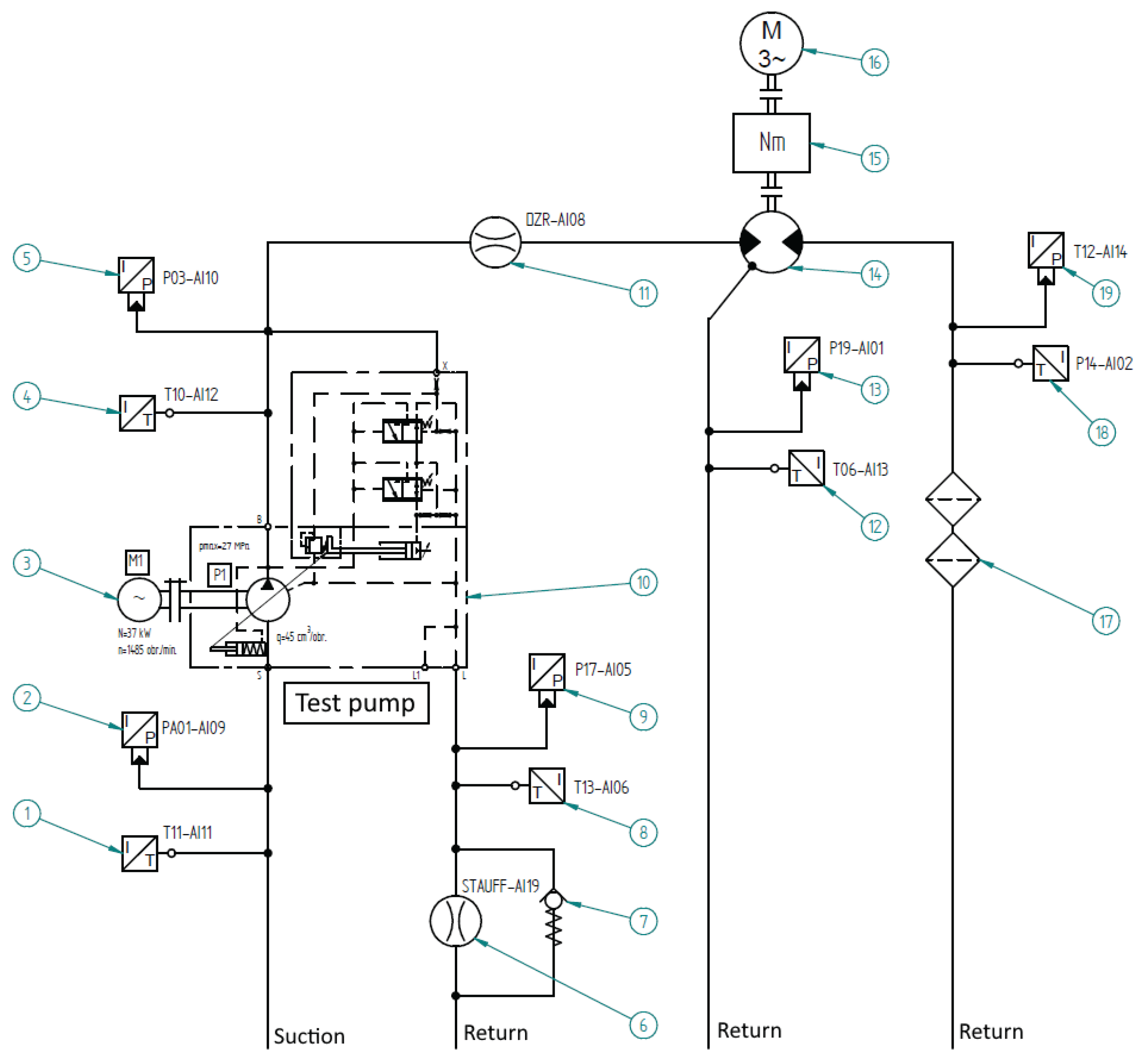
Figure 2.
Research setup photo showing the pump and the visualized locations of the vibrodiagnostic sensors.
Figure 2.
Research setup photo showing the pump and the visualized locations of the vibrodiagnostic sensors.
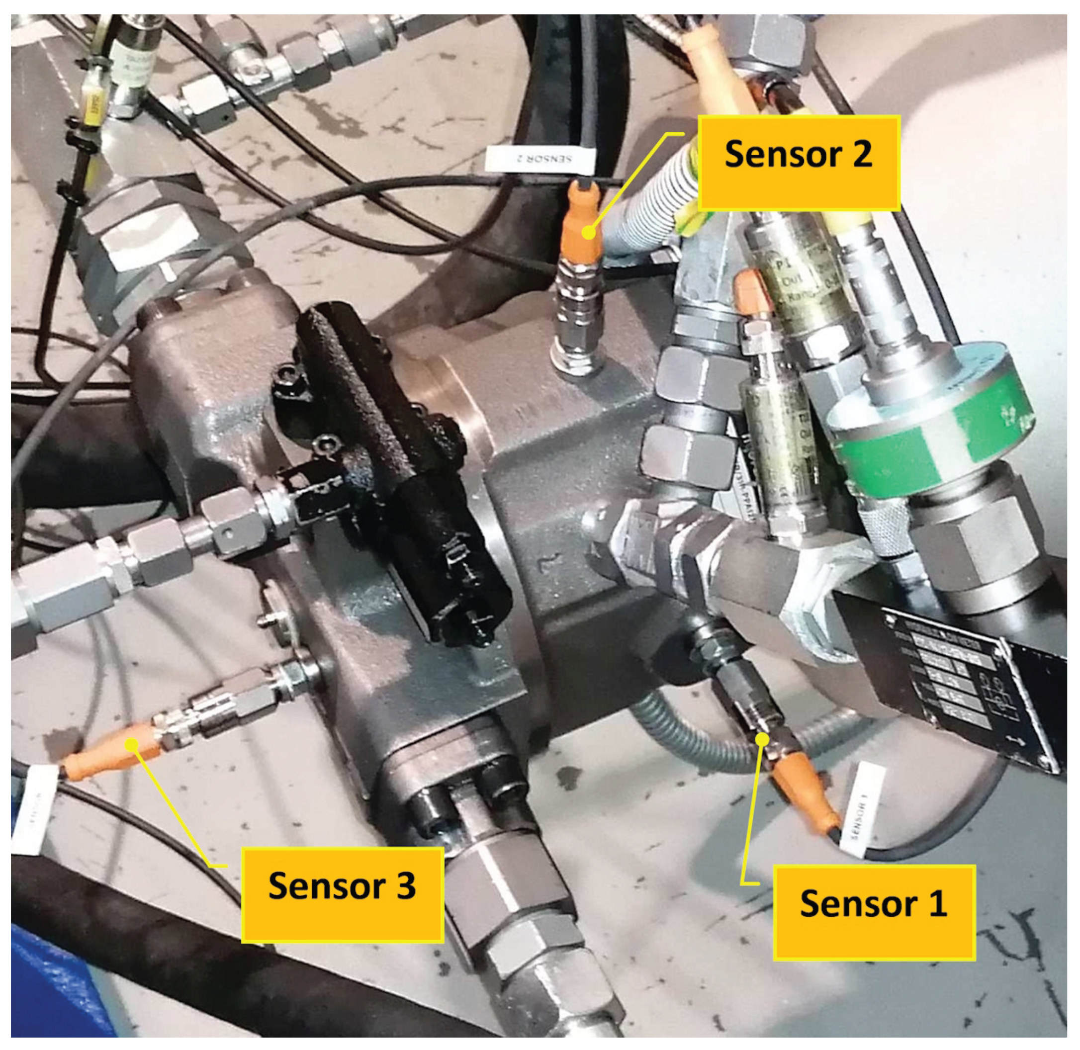
Figure 3.
Data processing pipeline including cross-validation test used in the experiments for parameter optimization and performance assessment on .
Figure 3.
Data processing pipeline including cross-validation test used in the experiments for parameter optimization and performance assessment on .
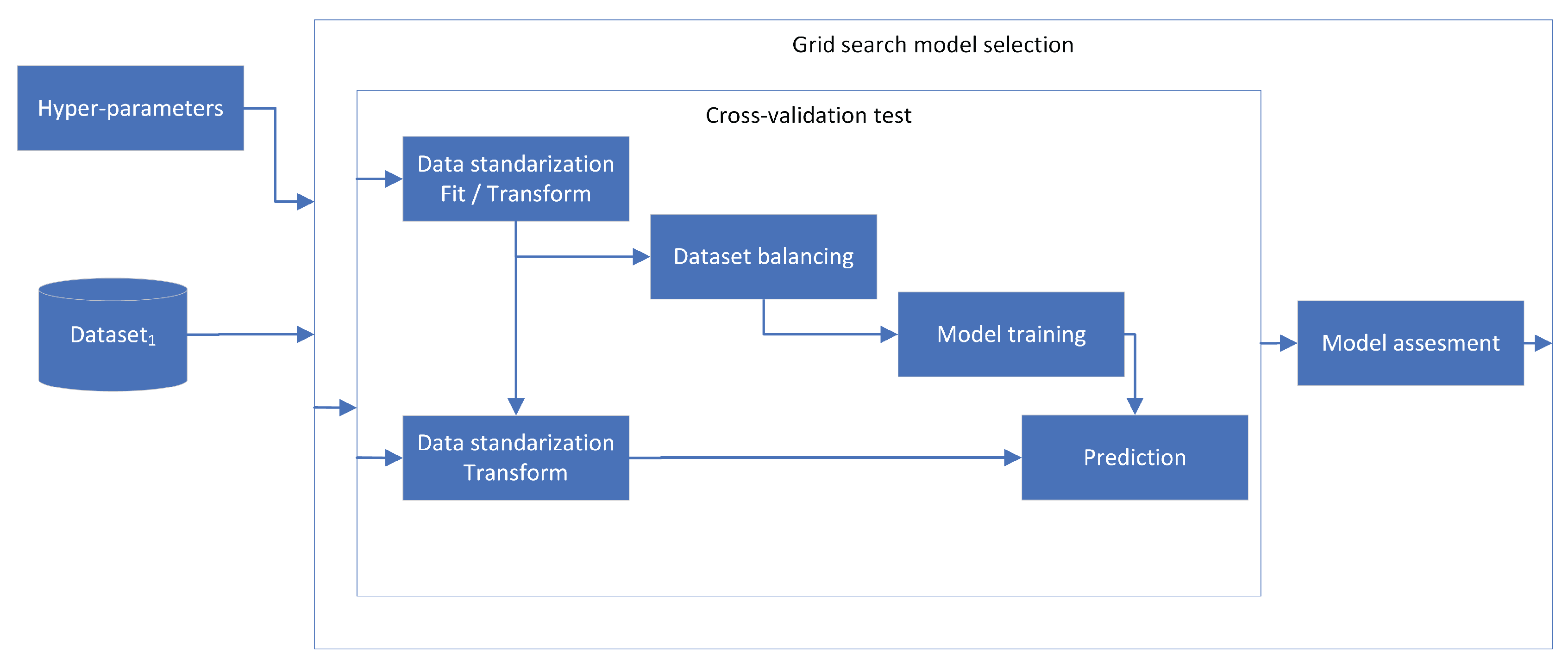
Figure 4.
Data processing pipeline used to asses the performance on and using model trained on .
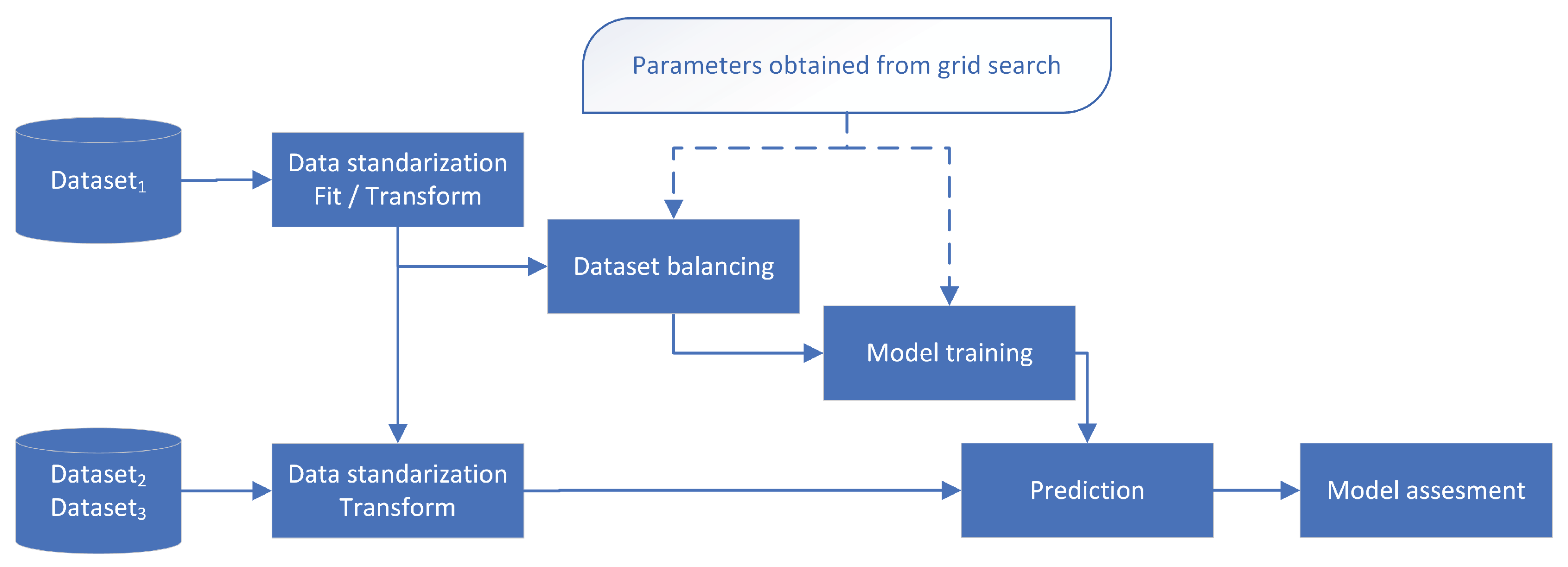
Figure 5.
An example of performance metric.
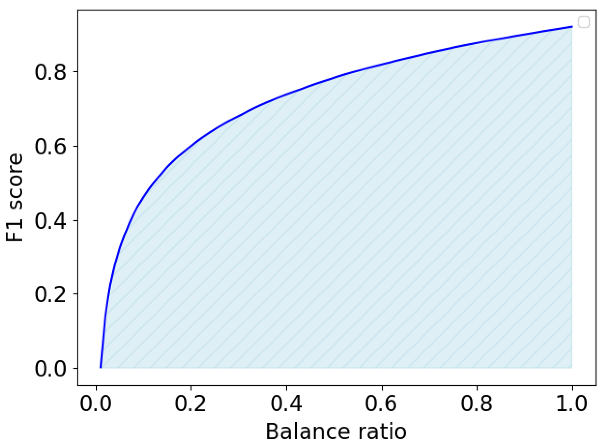
Figure 6.
The influence of the imbalance rate on the prediction performance (F1-score). Figure 6a Results on , Figure 6b Results on , Figure 6c Results on .
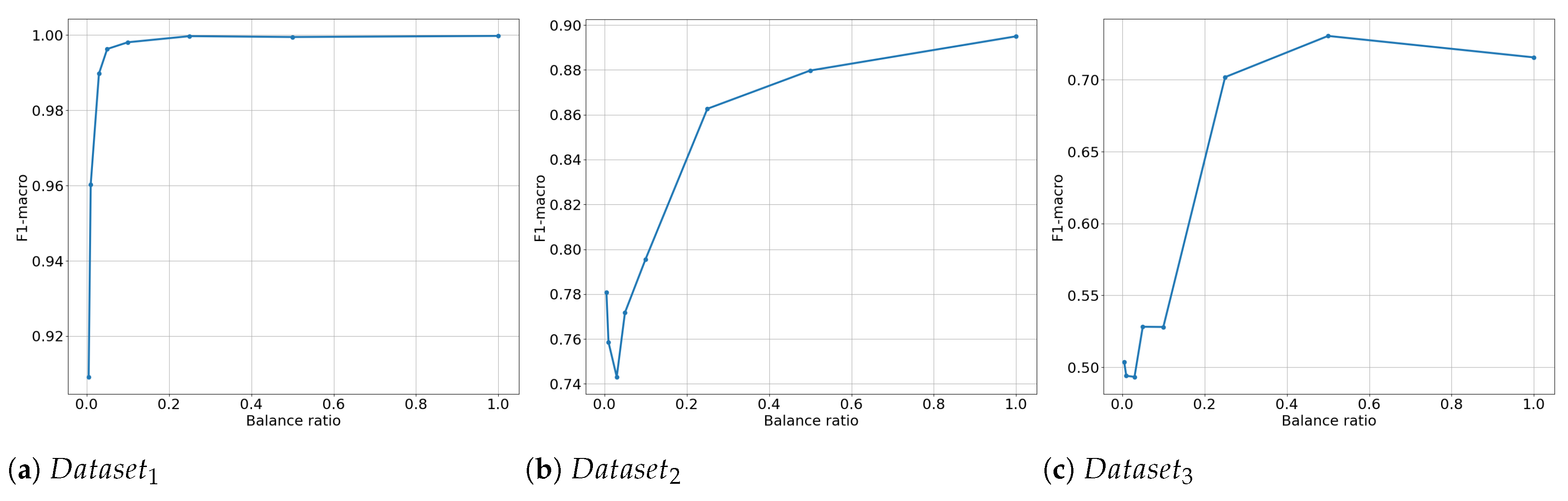
Figure 7.
Relation between models’ performance and the data balance ratio obtained when the model was trained on or a given balance rate and evaluated on: (a) (cross-validation procedure) (b) (c) .
Figure 7.
Relation between models’ performance and the data balance ratio obtained when the model was trained on or a given balance rate and evaluated on: (a) (cross-validation procedure) (b) (c) .
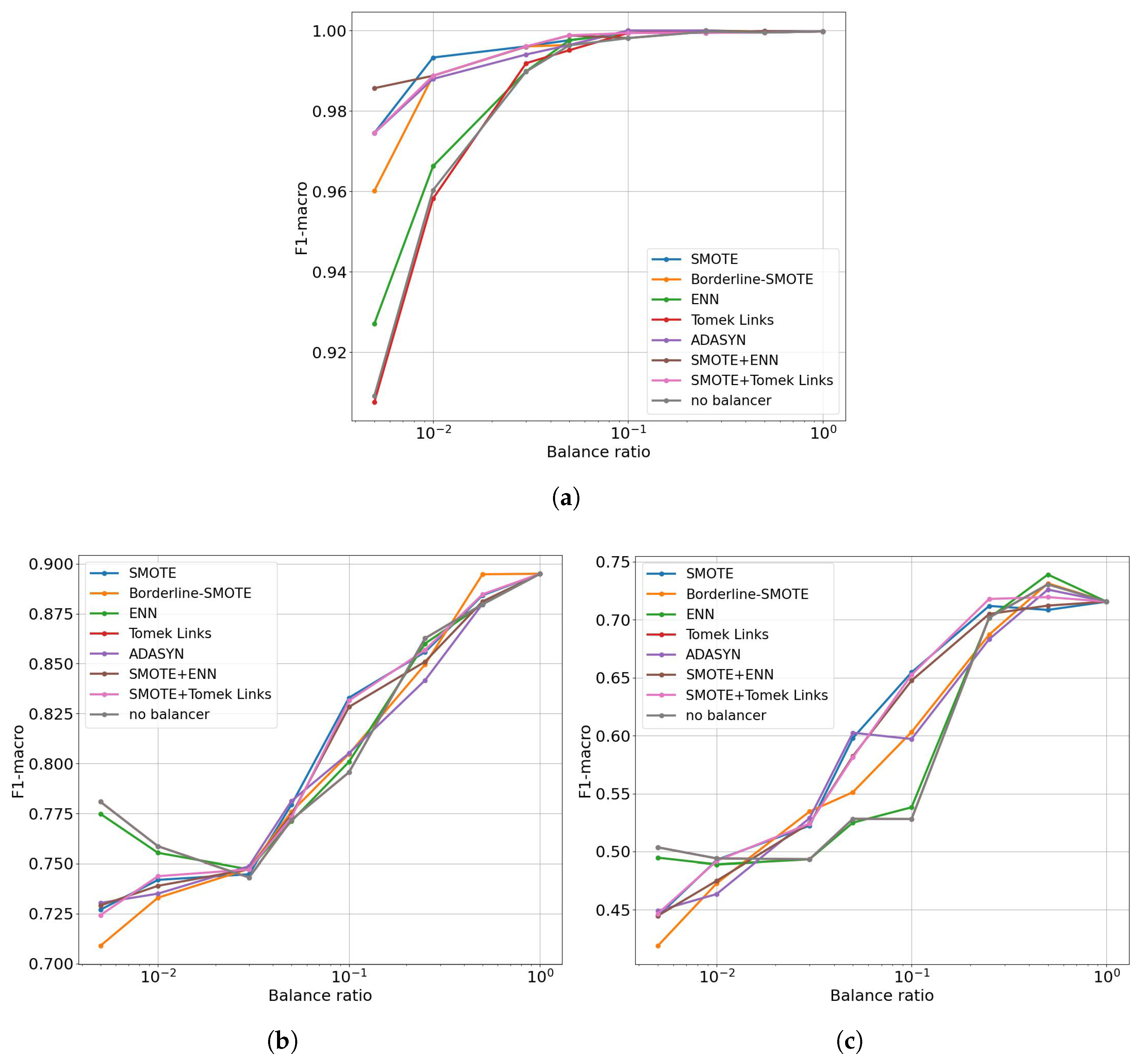
Figure 8.
Visualization of the BAUC metrics obtained for each data balancing method for each od the datasets: (a) . (b) . (c) .
Figure 8.
Visualization of the BAUC metrics obtained for each data balancing method for each od the datasets: (a) . (b) . (c) .
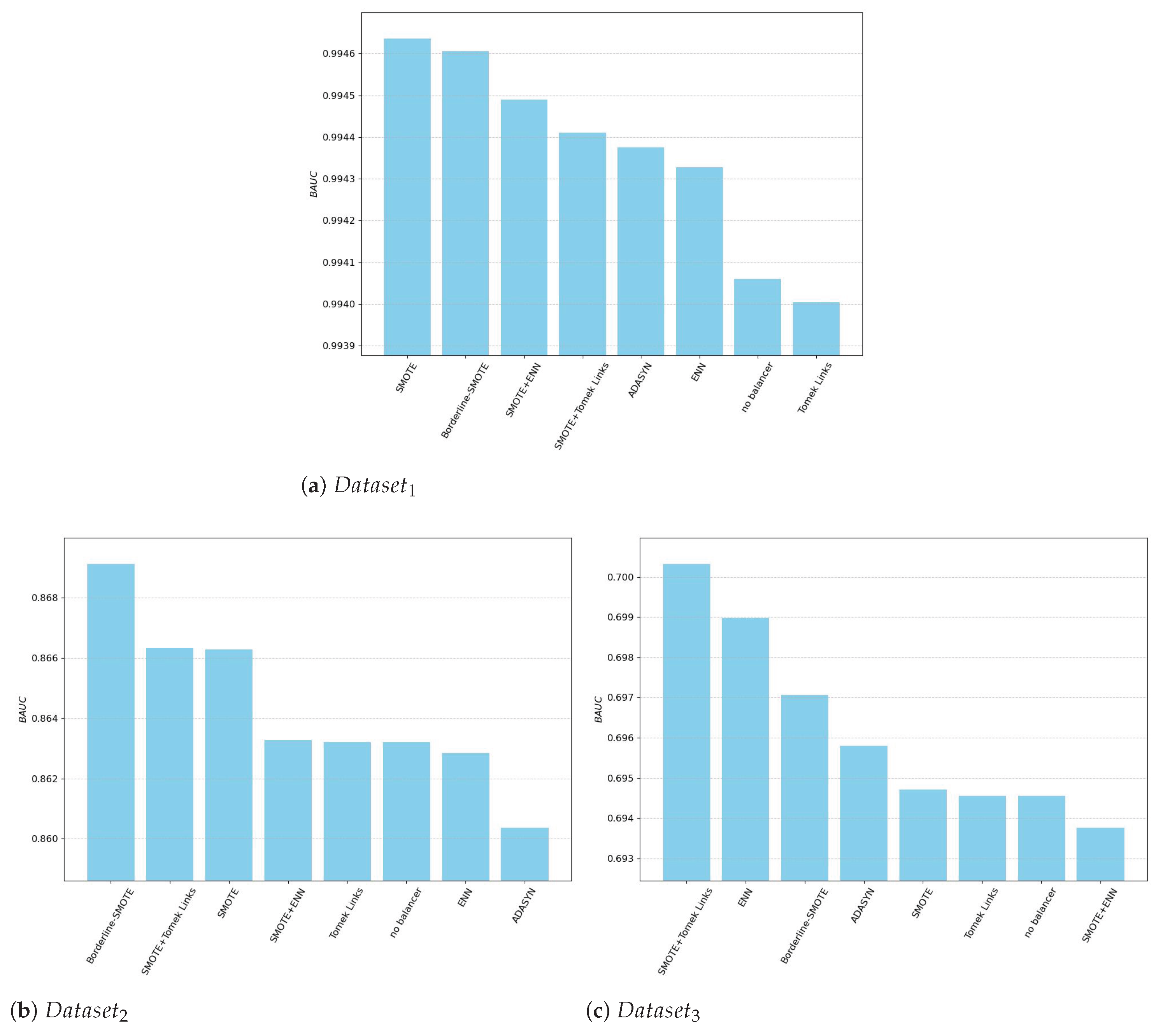
Figure 9.
Visualization of the input variable distributions using box plots for balance rates in the range . The figure shows that the distribution of the input variables for is noticeably different from the others, while for the remaining balance rates, the distributions are very similar.
Figure 9.
Visualization of the input variable distributions using box plots for balance rates in the range . The figure shows that the distribution of the input variables for is noticeably different from the others, while for the remaining balance rates, the distributions are very similar.
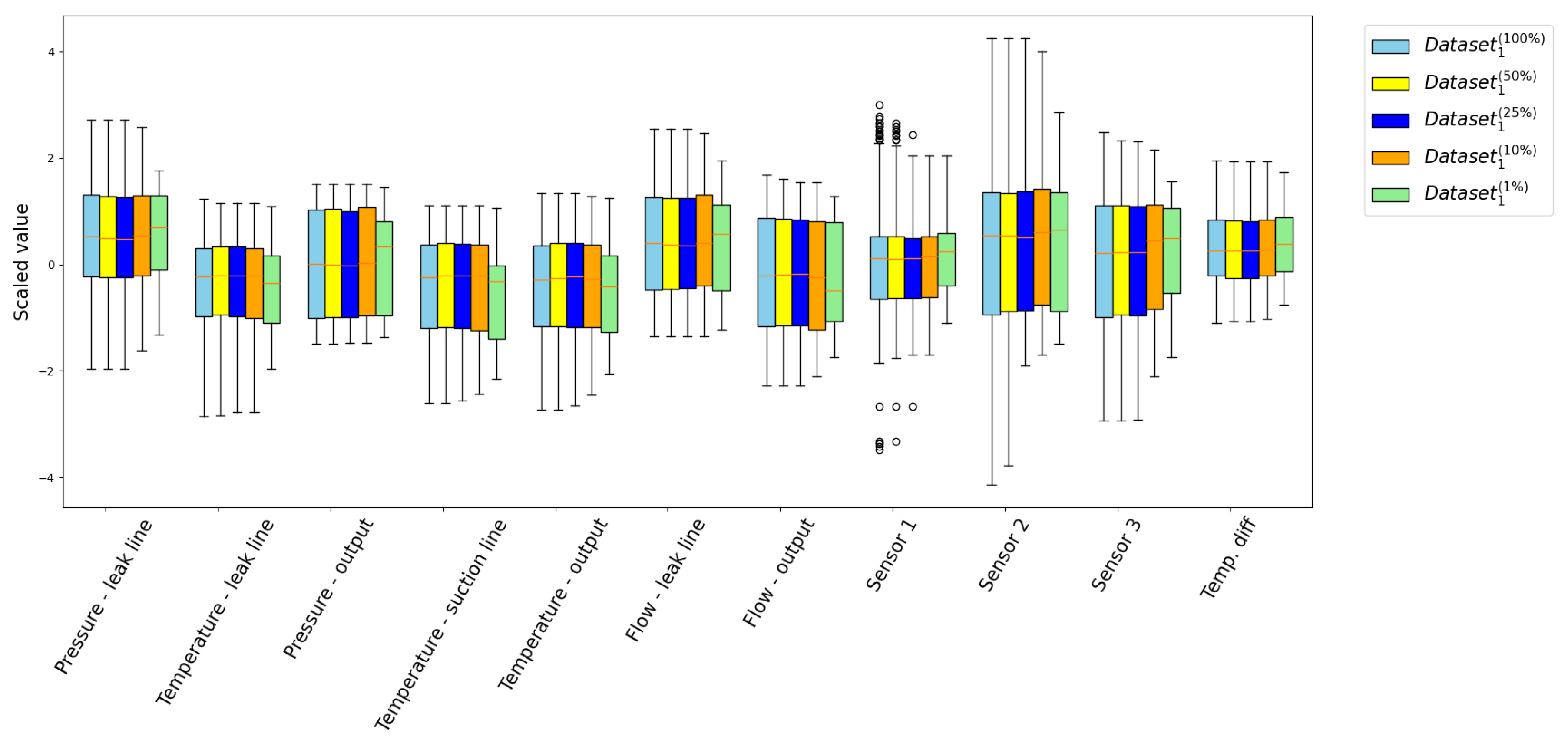
Figure 10.
Feature importance depending on balancing models for .
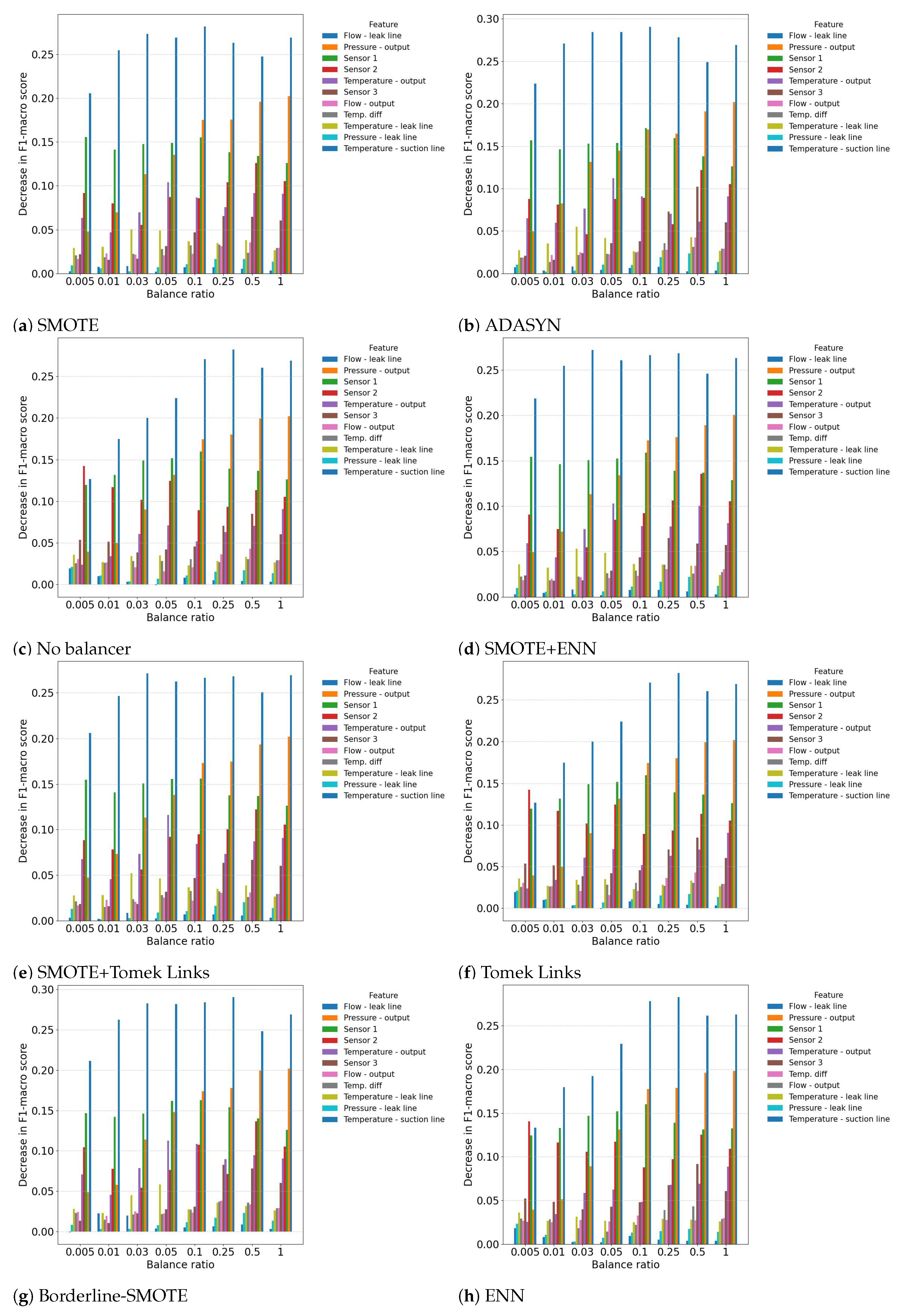
Figure 11.
Pearson correlation of balance ratio factors.
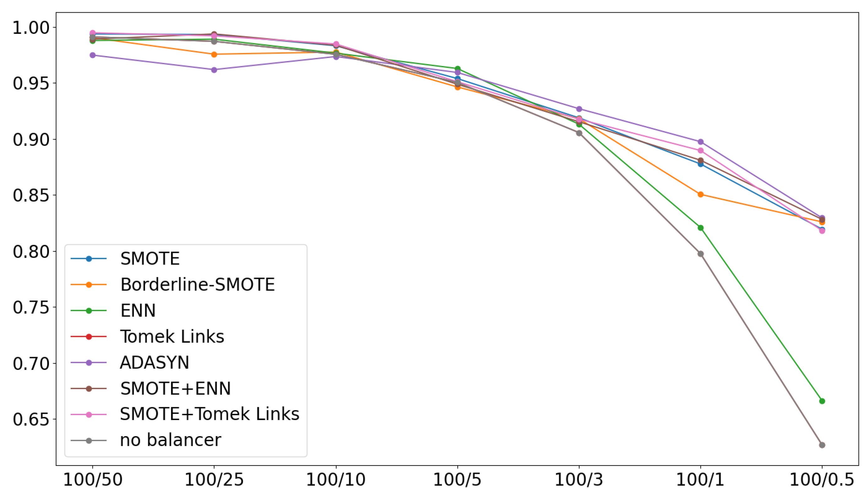
Table 1.
List of sensors used in the experiments.
| Pos. | Description | Symbol | Manufacturer |
|---|---|---|---|
| 1 | Temperature sensor Pt1000 150 °C | TA2105 | IFM, Germany |
| 2 | Pressure sensor -1…1 bar | PA3509 | IFM, Germany |
| 3 | Electric motor 37 kW | FCMP 225S-4/PHE | AC-Motoren, Germany |
| 4 | Temperature sensor Pt1000 150 °C | TA2105 | IFM, Germany |
| 5 | Pressure sensor 400 bar | PT5400 | IFM, Germany |
| 6 | Turbine flow meter | PPC-04/12-SFM-015 | Stauff, Germany |
| 7 | Check valve | S8A1.0 | Ponar, Poland |
| 8 | Temperature sensor Pt1000 150 °C | TA2105 | IFM, Germany |
| 9 | Pressure sensor 10 bar | PT5404 | IFM, Germany |
| 10 | Piston pump | HSP10VO45DFR | Hydraut, Italy |
| 11 | Gear wheel flow meter | DZR-10155 | Kobold, Germany |
| 12 | Temperature sensor Pt1000 150 °C | TA2105 | IFM, Germany |
| 13 | Pressure sensor 10 bar | PT5404 | IFM, Germany |
| 14 | Hydraulic motor | F12 060 MF | Parker, USA |
| 15 | Torque meter | T22/1KNM | HBM, Germany |
| 16 | Electric motor 170 kW | LSRPM250ME1 | Emerson, USA |
| 17 | Filter | FS1 | Ponar, Poland |
| 18 | Pressure sensor 250 bar | PT5401 | IFM, Germany |
| 19 | Temperature sensor Pt1000 150 °C | TA2105 | IFM, Germany |
| 20 | Vibration sensors 1 | VSA001 | IFM, Germany |
| 21 | Vibration diagnostic converter 1 | VSE100 | IFM, Germany |
1 Not shown in diagram.
Table 3.
Datasets used in the experiments.
| Dataset | Records Normal | Records Failure | Records Total |
|---|---|---|---|
| 4349 | 4349 | 8698 | |
| 4349 | 2174 | 6523 | |
| 4349 | 1087 | 5436 | |
| 4349 | 434 | 4783 | |
| 4349 | 217 | 4566 | |
| 4349 | 130 | 4479 | |
| 4349 | 43 | 4392 | |
| 4349 | 21 | 4370 | |
| 2887 | 2887 | 5774 | |
| 2887 | 2887 | 5774 |
Table 4.
Prediction performance obtained by the best performing neural network for each of the datasets. Scores F1-macro.
Table 4.
Prediction performance obtained by the best performing neural network for each of the datasets. Scores F1-macro.
| Model | |||
|---|---|---|---|
| MLP((40,20)) | 90.14 | 89.50 | 71.56 |
Table 5.
Average models ranking with BAUC scores.
| Model |
Rank |
Rank |
Rank |
Average Rank |
|||
|---|---|---|---|---|---|---|---|
| Borderline-SMOTE | 0.99461 | 0.86911 | 0.69706 | 2.0 | 1.0 | 3.0 | 2.0 |
| SMOTE+Tomek Links | 0.99441 | 0.86634 | 0.70032 | 4.0 | 2.0 | 1.0 | 2.3 |
| SMOTE | 0.99464 | 0.86627 | 0.69471 | 1.0 | 3.0 | 5.0 | 3.0 |
| ENN | 0.99433 | 0.86284 | 0.69898 | 6.0 | 7.0 | 2.0 | 5.0 |
| SMOTE+ENN | 0.99449 | 0.86327 | 0.69376 | 3.0 | 4.0 | 8.0 | 5.0 |
| ADASYN | 0.99438 | 0.86037 | 0.69580 | 5.0 | 8.0 | 4.0 | 5.7 |
| no balancer | 0.99406 | 0.86320 | 0.69456 | 7.0 | 5.5 | 6.5 | 6.3 |
| Tomek Links | 0.99400 | 0.86320 | 0.69456 | 8.0 | 5.5 | 6.5 | 6.7 |
Disclaimer/Publisher’s Note: The statements, opinions and data contained in all publications are solely those of the individual author(s) and contributor(s) and not of MDPI and/or the editor(s). MDPI and/or the editor(s) disclaim responsibility for any injury to people or property resulting from any ideas, methods, instructions or products referred to in the content. |
© 2025 by the authors. Licensee MDPI, Basel, Switzerland. This article is an open access article distributed under the terms and conditions of the Creative Commons Attribution (CC BY) license (http://creativecommons.org/licenses/by/4.0/).
Copyright: This open access article is published under a Creative Commons CC BY 4.0 license, which permit the free download, distribution, and reuse, provided that the author and preprint are cited in any reuse.


