Submitted:
12 September 2025
Posted:
15 September 2025
You are already at the latest version
Abstract
With the growing advantages and conveniences provided by digital transactions, the financial sectors also face a loss of billions of dollars each year. While the use of credit cards has made life easier and convenient, it has also become a significant threat. Detecting fraudulent transactions in financial sectors like banking is a major issue because the existing fraud detection methods are rule-based and unable to detect unknown patterns because the tactics and the techniques used by fraudsters are way more advanced then they are, making machine learning (ML) a valuable approach to improve detection efficiency. The present study implements and compares the performances of two widely used ML algorithms, Random Forest (RF) and Extreme Gradient Boosting (XGBoost), to identify credit card fraud. To improve model transparency and interpretability, two explainable AI techniques, SHapley Additive exPlanations (SHAP) and Local Interpretable Model- Agnostic Explanations (LIME), are applied. A real-world credit card dataset is used to evaluate both models based on the standard key metrics such as accuracy, precision, recall, and interoperability. This study supports the integration of explainable artificial intelligence (XAI) into fraud detection systems to improve trust, reliability, and real-world applicability in the financial sector. These findings will help to choose the best model among them for the best scenario in the real world.
Keywords:
online transaction fraud
; machine learning
; random forest
; XGBoost
; SHAP
; LIME
; Explainable Artificial Intelligence (XAI)
; fraud detection
; model interpretability
; explainability
1. Introduction
In today’s digital world, the use of digital payments has made life easier in terms of time saving and convenience. For example, one can pay the bill, do online shopping, and make transactions through online payment. But these advancements have also given rise to very critical issues like fraud, financial loss, and privacy concerns, where fraudsters can steal one’s sensitive card information and use it to their advantage. These online transaction frauds are hard to detect because the card is not physically available, and the existing fraud detection methods are rule based means that they can only detect known fraud. There is a need for a technique that can detect unknown patterned fraud because the tactics and techniques use for fraud are way more advanced than existing methods. If this problem is not addresses on time , users might stop trusting on these digital transaction methods.
Machine learning can play a vital role in this because it allows the ability to learn and understand complex, unknown patterns, which is crucial for detecting fraudulent activities. Machine learning (ML) models, particularly Random Forest (RF) and Extreme Gradient Boosting (XGBoost) [1], have proven effective in detecting fraudulent transactions [2] because these works best for numerical features. Online transactions have become the mode of payment today, and while providing many facilities, it also introduced many challenges. Although prior studies [3] have compared the performance of Random Forest and XGBoost and mentioned the need for model interpretability, few have explored their interpretability using SHAP and LIME in the context of financial fraud detection, mostly focusing on just XGBoost.
The lack of model interpretability [4] remains a major challenge for the practical deployment of these models in financial systems, making it difficult to understand why a certain transaction is labeled as legitimate and or fraud by the model. Interpretability and explainability are not just features, but are regulatory and ethical necessities because in high-stakes domains like banking, financial institutions are often required to justify automated decisions to stakeholders, auditors, and end users. As such, the ability to explain model predictions enhances trust in these digital payment modes, easy troubleshooting, and helps in decision making. XAI Techniques like, SHAP and LIME provide insight into which features influence individual predictions, enabling domain experts to validate outcomes and uncover potential biases. Incorporating interpretability and explainability into machine learning techniques could help in enhancing the technical performance and real-world usability. This integration could help in the real world for detecting fraudulent transactions.
This paper aims to fill this gap by implementing and comparing the performance of both models on a real-world credit card fraud dataset using standard evaluation metrics such as accuracy, precision, recall, and explainability as key evaluation metrics. The results will help to understand which models perform well in which scenario and to select the best model according to the requirements in the real world. These findings will offer insights into the trade-off between performance and explainability and will provide valuable guidance for deploying machine learning models in real-world financial fraud detection systems.
The remainder of this paper is organized as follows: Section 1 provides the Introduction. Section 2 reviews the Related Work on fraud detection and explainable machine learning. Section 3 describes the Materials and Methods, including the implementation details of the proposed techniques with SHAP and LIME. Section 4 presents the Results. Section 5 provides a Comparative Analysis of the proposed models. Section 6 offers the Discussion and Analysis. Finally, Section 7 concludes the study and outlines directions for future research.
2. Related Work
2.1. Traditional Methods for Credit Card Fraud Detection
Credit card fraud is a growing challenge in financial transactions, particularly in the context of online payment systems, as it has become a mode of payment. Online transaction fraud is hard to detect as the card is not physically available. Many traditional fraud detection system are available, such as, rule based, statistical methods, and blacklist whitelist. These methods heavily rely on known patterns, making them not suitable for such types of fraud because the techniques used for fraud are now more advanced than these methods. Researchers [5] have focused on developing systems that can detect fraudulent behavior based on transaction patterns, using both traditional statistical methods and machine learning techniques but there finding suggest that these methods are not helpful and causes reputational damages, financial losses, and highlighted the need for more robust and adaptive fraud detection methods. This has led to a move towards machine learning (ML) models, which can adapt to new fraud patterns by learning from previous transaction data.
Another study [6] concludes that traditional ruled based systems are increasingly ineffective in detecting modern fraud attacks because these can be reversed and often generates high false positives and false negatives, which directly causes missing real threats. The rule-based systems are too rigid and unsuitable to tackle modern frauds [7] as they are not adaptable. This study highlighted the need for ML-based techniques because traditional methods cannot learn from past behaviors and experiences.
2.2. Machine Learning Approaches for Credit Card Fraud Detection
Researchers in [8] conducted a comprehensive survey of ML methods for fraud detection and highlighted the problem of imbalanced data and how it affects the overall performance of the model. This study also mentioned the need for an explainable system and the hybrid approach can enhance the performance of fraud detection systems. However, a key challenge remains in understanding model decisions, particularly in regulatory-compliant industries like banking [9] compared various ML algorithms and data balancing techniques, including SMOTE, ADASYN, and NCR, for handling highly imbalanced fraud detection datasets. Their findings indicated that XGBoost with Random Oversampling achieved the highest F1-score (92.43 per), followed closely by Random Forest with similar techniques.
However, the study did not explore the interpretability of these models, which is crucial for practical deployment. [10] introduced the unsupervised framework for credit card fraud detection, combining SHAP (Shapley Additive exPlanations) for feature selection and an autoencoder-based approach for generating class labels. This method is designed to handle common challenges in fraud detection, such as extreme class imbalance, data privacy, and the scarcity of labeled data. The authors first applied SHAP to rank feature importance without using any labels, making it suitable for unsupervised learning, and then an autoencoder was trained to compute reconstruction errors on the unlabeled dataset, assigning high-error transactions as fraudulent. To evaluate the quality, Decision Tree, Random Forest, Logistic Regression, and MLP were trained on the newly labeled data. Their results suggest that unsupervised learning techniques are to best suitable for numerical feature datasets, and the model only provides the global importance of the feature importance as only SHAP was used, and the explanation results are less interpretable. In this approach [11], SHAP was used with Isolation Forest to evaluate feature importance without relying on labeled data. Models trained using only the top 15 SHAP-selected features achieved performance comparable to, and in some cases better than, models using the full feature set, as evaluated using AUPRC and AUC metrics.
2.2.1. Deep Learning and Hybrid Approaches
Deep learning models such as ResNeXt and Gated Recurrent Units (GRU) for fraud detection were explored by [12] and compared their results with traditional machine learning models. Despite their success in performance metrics, these deep learning models lacked interpretability, which makes it difficult to understand the decision of model. Similarly, in [13] integrate Graph Neural Networks (GNN) and Autoencoders for fraud detection, and their results declared high performances, but the inherent complexity of these models raised concerns about their transparency and real-world deployment in banking systems. In [14] explored RF and XGBoost against deep learning models. Their study revealed that while deep networks can capture complex fraud patterns but RF and XGBoost remain preferable for real-time fraud detection due to their computational efficiency and interpretability.
2.2.2. Ensemble Learning Techniques for Fraud Detection
Ensemble learning techniques are well-suited for numerical features because they provide high accuracy and improve classification. These methods have been widely used in fraud detection systems. The study [15] compared RF and XGBoost under varying class imbalance conditions and concluded that hyperparameter-tuned XGBoost consistently outperformed Random Forest in F1-score and precision. Despite these advantages, their study did not investigate the interpretability of these ensemble models, which leaves a critical gap in understanding how these models make decisions. Meta-Huristic optimization technique was used by [16]. This study demonstrated that this technique significantly improves feature selection and reduces false negatives in RF and XGBoost. The study [17] demonstrated that ensemble techniques perform better than other ML models as they are simple, require less data, and work well with explainability tools.
2.2.3. Explainable AI in Fraud Detection
Regulatory bodies such as finance and banking are often required to demonstrate the results to their stakeholders and end-users, as why a certain transaction was labeled as fraudulent by the model. Machine learning models perform very well in detecting complex patterns of fraud, but they often lack explainability and interoperability, which are crucial for real-life systems. The study [4] conducted a systematic literature review of ML-based financial fraud detection techniques and identified that credit card fraud is the most widely studied category. Their results highlighted that Random Forest is a frequently applied ensemble method due to its robustness in handling imbalanced data, but the major issue is the lack of model interpretability, and highlighted the need to use XAI tools to improve the model’s explainability. The study [18] applied SHAP and LIME into fraud detection frameworks on multiple ML models, excluding RF, and their results show that these techniques can enhance model transparency, improve feature attribution, and provide actionable insights for financial analysts. Another Study [19] introduced the XGBoost technique to highlight critical financial frauds, and the model employs SHAP (Shapley Additive Explanations) and LIME (Local Interpretable Model-agnostic Explanations) to enhance interpretability, which can help in understanding the final prediction of the model. Another study [20] explored SHAP for anomaly detection in financial systems, and their findings suggest that SHAP could help in increasing model interpretability. The study [21] demonstrated the application of SHAP and LIME in improving interpretability in ML models used for fraud detection. They implemented both models on urban remote sensing and compared them for land class mapping. Their study highlighted that while XGBoost exhibited superior accuracy, Random Forest offered better interpretability, making it more suitable for regulatory compliance, for example, earth observation.
Similarly, another study [22] provides a detailed examination of the ML-based approaches to fraud detection by grouping them into three primary categories: supervised, unsupervised, and hybrid models. Their results showed that supervised techniques such as Random Forest, XGBoost, Support Vector Machines (SVM), and Logistic Regression, have demonstrated strong performance when sufficient labeled data are available than unsupervised and hybrid approaches. However, their effectiveness can be compromised by severe class imbalance. To address this, the study recommends focusing on performance indicators such as precision, recall, F1-score, and AUC-ROC rather than overall accuracy.In contrast, unsupervised models like K-Means and DBSCAN are better suited for scenarios lacking labeled data but can help in detecting unusual fraudulent transactions.
A separate investigation [23] compares the performance of several classifiers, including Random Forest, Decision Tree, Naïve Bayes, Logistic Regression, K-Nearest Neighbors, and SVM, using a real-world dataset characterized by a significant class imbalance. Random Forest exhibits effective results, achieving precision and recall rates of 0.98 and 0.93, respectively. The authors employed SMOTE (Synthetic Minority Oversampling Technique) during preprocessing to handle class imbalance. Despite the high accuracy of ensemble models, the study noted potential drawbacks such as limited model interpretability and challenges in adapting to new types of fraud.
The study [24] compared the performance of XGBoost and logistic regression and demonstrated that XGBoost significantly outperform in detecting fraudulent bank transactions and highlights the importance of feature engineering and metrics like Somers’ D/AUC for handling imbalanced datasets. XGBoost effectively reduces both false positives and false negatives also enhancing fraud detection accuracy while improving operational efficiency and regulatory compliance. However, challenges such as model interpretability and data dependency remain unaddressed. The paper [25] highlights the importance of XAI tools in making the systems more transparent, efficient, trustworthy, and accountable, but also the challenges remain in balancing accuracy, interpretability, and ethical considerations. The study suggests that future research should focus on creating standardized, user-centric XAI frameworks to bridge the gap between complex AI models and human understanding.
Machine learning techniques, particularly ensemble models like Random Forest and XGBoost, have shown great potential in fraud detection due to their ability to analyze large volumes of data, identify hidden patterns, and these techniques work well with numerical features. While these models offer high accuracy and efficiency, a significant challenge remains, which is their lack of interpretability. This study [26] employs Random Forest (RF) and XGBoost for credit card fraud detection. The authors report RF achieving an F1-score of 85.71 %(precision: 97.40 %, recall: 76.53% ) and XGBoost attaining 85.3 %, F1-score (precision: 95.00%, recall: 77.55 per). While their hybrid model outperforms, the paper does not address interpretability techniques like SHAP/LIME, which our study explicitly incorporates to enhance model transparency.
The paper [27] focused on improving fraud detection systems using machine learning, particularly ensemble methods. It addresses key challenges such as data imbalance, computational efficiency, and real-time processing, proposing a novel ensemble model combining SVM, KNN, Random Forest, Bagging, and Boosting but lack interpretability. The present study aims to address this gap by not only implementing and evaluating the results of both models, Random Forest and XGBoost, to decide which model detects frauds efficiently, but also to use XAI tools, SHAP and LIME, to evaluate their explainability. The goal of this study is to help in deciding the best model that can detect fraudulent transactions, as well as can also help understand the prediction of the model in real-world applications in the financial sector.
3. Materials and Methods
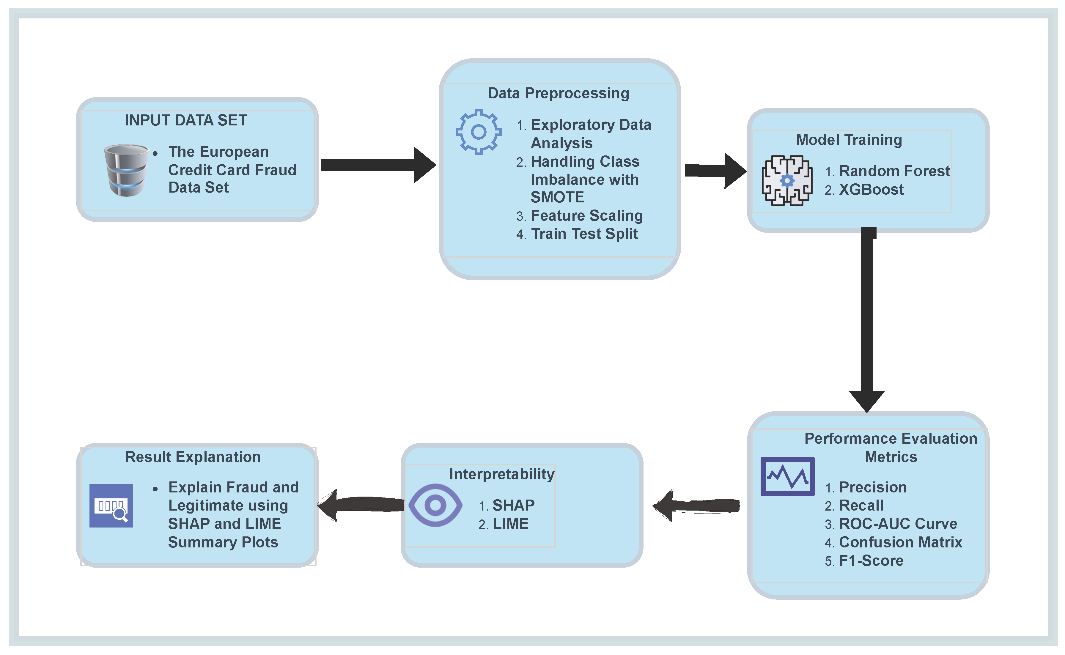
This study aims to implement and compare the performance of two popular machine learning models, Random Forest (RF) and XGBoost, for the detection of credit card fraud in online transactions. Additionally, to enhance the interpretability and explainability of these models, SHAP (SHapley Additive Explanations) and LIME (Local Interpretable Model-Agnostic Explanations) were used, which are XAI tools. The chosen approach will allow us to assess not only the accuracy and efficiency of the models but also their transparency, which is crucial for deploying machine learning solutions in financial sectors. The first step was the preprocessing of the credit card fraud detection dataset, followed by training the Random Forest and XGBoost models. The models will be evaluated using common standard classification metrics such as accuracy, precision, recall, F1 score, and ROC-AUC and the key metric is interpretability. To ensure that the results are interpretable, SHAP and LIME will be utilized to explain the models’ predictions and to understand which features most influence the classification decisions. Comparison of these models will help identify the most effective approach for online transaction fraud detection while maintaining transparency and interoperability. This will also helps in gaining and maintaining end user trust in these digital payment methods, but also helps explain the model’s prediction to stakeholders and end users.
Figure 1.
Proposed Methodology for Credit Card Fraud Detection using Random Forest and XGBoost with SHAP and LIME
Figure 1.
Proposed Methodology for Credit Card Fraud Detection using Random Forest and XGBoost with SHAP and LIME
3.1. Data Set
The study uses the European Credit Card Fraud Detection Dataset from Kaggle, which contains anonymized transactions in the real world. The dataset includes 284,807 transactions with 492 fraudulent cases, making it highly imbalanced. Features are numerical due to PCA transformation, with the ’Class’ column indicating fraud (1) or legitimate (0) transactions.

Table 1.
Sample of Credit Card Transaction Dataset
| Time | V1 | V2 | V3 | ... | Amount | Class |
|---|---|---|---|---|---|---|
| 0.0 | -1.3598 | -0.0728 | 2.5363 | ... | 149.62 | 0 |
| 0.0 | 1.1918 | 0.2661 | 0.1664 | ... | 2.69 | 0 |
| 1.0 | -1.3583 | -1.3401 | 1.7732 | ... | 378.66 | 0 |
3.2. Data Processing
The selected dataset needs to pass through some steps before training the models on it. These steps help in organizing the features and making efficient predictions. The steps are:
3.2.1. Standardization
As the dataset contains many features and they might have different scales. If all features are not scaled in a standard way, the model will give high priority to large-scale features, making it difficult for the model to predict correctly. To solve this problem, numerical features are scaled using StandardScaler to ensure uniformity.The following equation is used by the StandardScaler to normalize the features:
where:
- x: the original value of a feature
- : the mean of the feature
- : the standard deviation of the feature
- z: the standardized (normalized) value
3.2.2. Data Splitting
The dataset is divided into 80% training and 20% testing. This is the balanced division of the dataset, as the model will get trained on enough data and learn complex patterns and also enough data to for evaluation. T following equations demonstrated the splitting of the dataset:
3.2.3. Oversampling
The dataset contains the majority of legitimate cases. Only about 0.17% fraud cases. This makes the dataset highly imbalanced. The models would not be able to differentiate between the fraudulent and legitimate transactions. AS there are high numbers of non-fraudulent transactions, the models will interpret all of them as legitimate. To overcome this problem, SMOTE (Synthetic Minority Oversampling Technique) was applied to the training set to synthetically generate minority class samples and improve model performance. SMOTE tackles this issue by generating artificial fake samples and adding noise for the underrepresented class. This process enhances the number of minority class instances, which results in a more balanced dataset. Such balancing can lead to improved model performance, especially in scenarios involving imbalanced classification problems.
where:
- : samples of the majority class (legitimate transactions)
- : original samples of the minority class (fraudulent transactions)
- : synthetic samples generated using SMOTE
3.3. Machine Learning Models
The present study uses the two most powerful models of machine learning. These models perform very well for numerical features, handle imbalance, and avoid overfitting. The models are:
3.3.1. Random Forest (RF)
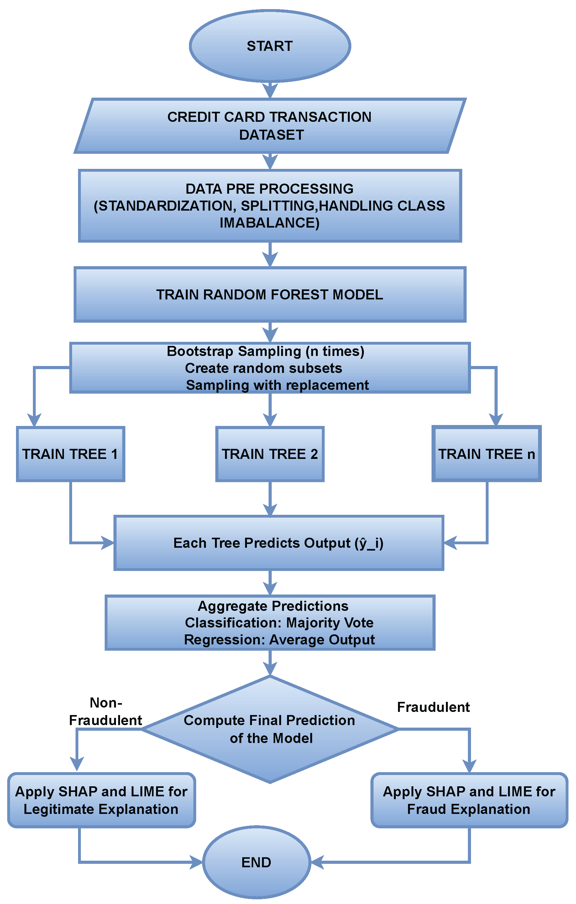
An ensemble machine learning technique that is widely used for classification problems. The main goal of it is to reduce overfitting and increase generalization. It trains multiple trees on different subsets of the dataset to avoid overfitting, and after each tree predicts its result, it starts aggregating them. Majority voting is used to predict the final result. Once the decision trees are built, they can be used to make predictions. For classification tasks, each tree in the forest casts a “vote” for the class label, and the final prediction is based on the majority vote from all the trees. For regression tasks, the average prediction of all the trees is taken.
3.3.2. Random Forest Algorithm
Random Forest is an ensemble learning method that operates by constructing multiple decision trees at training time and outputting the class that is the mode of the classes (classification) or mean prediction (regression) of the individual trees.
3.3.3. Random Forest for Classification
The Random Forest classifier predicts a class label by aggregating the predictions from B decision trees , where each tree is trained on a bootstrap sample of the data:
where:
- x: Input feature vector
- : Prediction from the b-th decision tree
- B: Total number of trees in the forest
- : Final predicted class label
3.3.4. Bootstrap Aggregating (Bagging)
Each tree in the Random Forest is trained on a different bootstrap sample, a subset of the dataset. Bagging helps to reduce the variance of the model without increasing the bias. The bootstrap sample for tree b is created by sampling with replacement from the original training dataset. Mathematically, it can be represented as:
where:
- is the final predicted class label for input x (e.g., fraud or not fraud),
- is the prediction made by the b-th decision tree in the ensemble,
- B is the total number of trees in the Random Forest,
- returns the most frequent (majority) class among all predictions.
Figure 2.
Working Flow Chart of RF with SHAP and LIME
3.3.5. Feature Randomness
At each split in a decision tree, a random subset of features is considered, which introduces diversity among the trees and improves generalization. If there are p total features, a subset of m features (typically for classification) is randomly selected at each split.
where:
- F is the full set of input features,
- is the randomly selected subset of features used at a split,
- m is the number of features chosen randomly for each split (),
- This randomness ensures that each decision tree explores different feature combinations, increasing model diversity.
3.3.6. Final Prediction (Probabilistic Form)
For probabilistic output (e.g., ROC AUC, SHAP explanations), the final predicted probability for class c is the average of the predicted probabilities from each tree:
where:
- : Probability output for class c from tree b
3.3.7. Interpretability Analysis of Random Forest using SHAP and LIME
To enhance the interpretability and explainability of Random Forest, two XAI tools were used. These techniques help to understand the prediction of the model and help in decision-making. Mathematically, the SHAP value for a feature can be represented as:
For Random Forest, shapley values will be calculated using TreeSHAP algorithm by examining the tree structure. Each feature prediction will contribute in the local and global importance of the feature.
Lime provides local explainability of the model’s decision. It generates perturbed samples around the ask the Random forest to make predictions again. It fits a linear model and selects the final feature based on the weights. Mathematically, the LIME value can be represented as :
3.3.8. XGBoost (XGB)
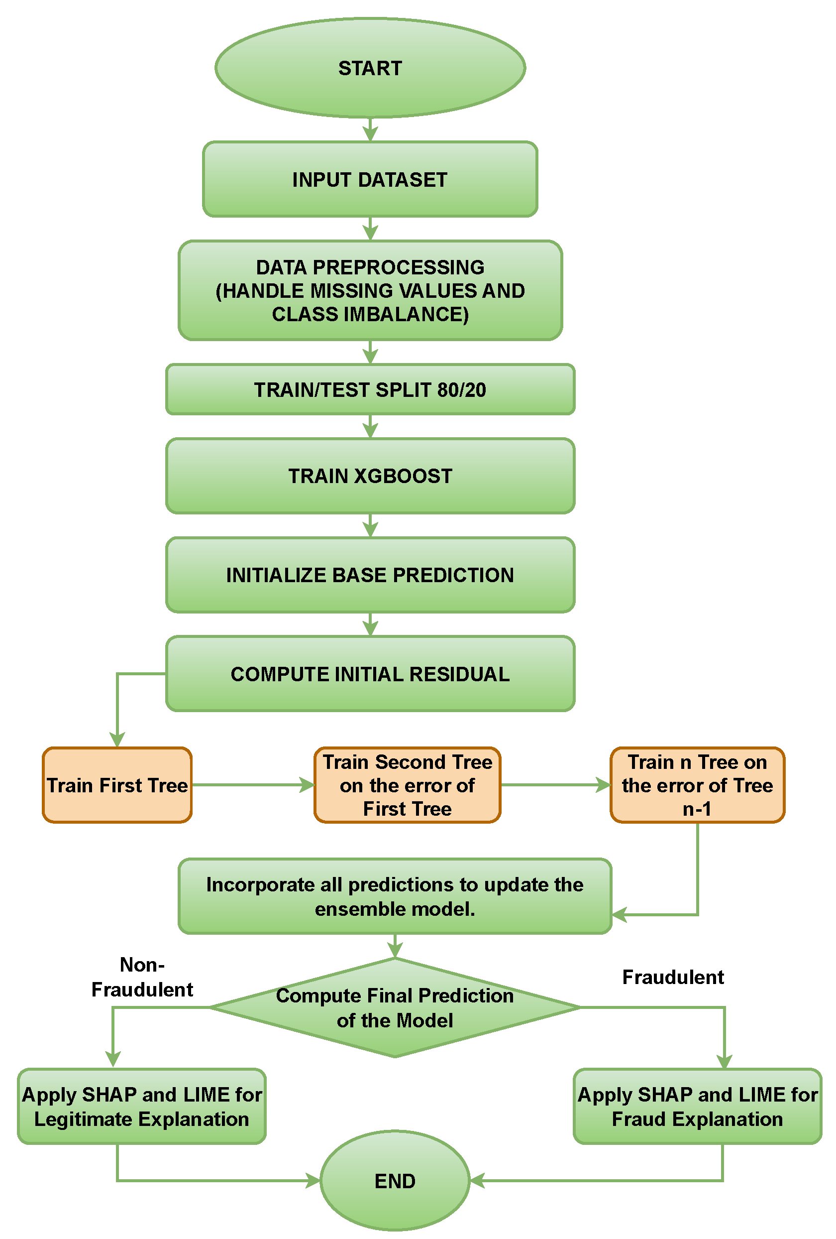
Extreme Gradient Boosting is an advanced machine learning algorithm that is widely used for both classification and regression. It is known for handling class imbalance effectively. It is an optimized implementation of gradient boosting, which is a machine learning technique where models are built sequentially, with each new model aiming to correct the errors made by the previous models.
3.3.9. XGBoost Algorithm
Extreme Gradient Boosting (XGBoost) is an efficient and scalable implementation of the gradient boosting framework. It is particularly powerful for tabular data. The objective function in XGBoost combines a loss function that measures the model’s performance and a regularization term to penalize complexity.
Figure 3.
Working of XGBoost with SHAP and LIME
3.3.10. Objective Function
It is used to balance prediction error and model complexity. It helps the model to improve at each boosting iteration. The overall objective function of XGBoost is given by:
where:
- : Total loss (objective function)
- : Differentiable convex loss function that measures the difference between the prediction and the actual label
- : Regularization term for the k-th tree
- : Space of regression trees
3.3.11. Regularization Term
The regularization function helps control model complexity and avoid overfitting. It is defined as:
where:
- T: Number of leaves in the tree
- : Score on leaf j
- : Penalty for each leaf (controls tree complexity)
- : L2 regularization term on leaf weights
3.3.12. Prediction Update
At each boosting iteration t, a new tree is added to update the prediction:
where:
- : Updated prediction after iteration t
- : Output of the new regression tree at step t
XGBoost optimizes this objective using a second-order Taylor approximation and greedy tree construction with pruning and regularization.
3.4. Performance Metrics
Standard key evaluation metrics will be used to evaluate the performance of each model. These metrics will help to compare and select the best model for a real-world scenario among them. The following are the key metrics used by the present study:
3.4.1. Accuracy
It is a fundamental metric used to evaluate the performance of classification models. It measures how often the model’s predictions are correct across all the predictions. Mathematically, accuracy is calculated as:
where:
- TP: Number of Correct Predictions
- TN: Number of correct False Predictions
- FN: Number of false negatives Predictions
- FP: Number of false positive Predictions
3.4.2. Precision
It is used to evaluate the performance of binary classification models. It measures the proportion of correct positive predictions. It evaluate that the correct predictions made by the model are actually correct. The formula for Precision is:
3.4.3. Recall
It is used to identify positive instances. It measures the proportion of actual positive instances that the model correctly identifies as positive. The formula for Recall is:
3.4.4. F1-Score
it provides the balance between the precision and recall by combining their values. In an imbalanced dataset where both false positives and false negatives are crucial to reduce, this metric provides many advantages. The F1-Score is the harmonic mean of precision and recall and ensures that a model performs well on both metrics. The formula for F1-Score is:
3.4.5. ROC-AUC
A graphical representation of the model performance in an imbalanced dataset. The AUC-ROC curve provides insights into the model’s ability to distinguish between the fraudulent and legitimate classes. It describes how well the model can differentiate between the true positive rate and false positive rate.
3.4.6. Model Interpretibility Using SHAP and LIME Plots
SHAP plots are used to represent the global and local importance of features in finalizing the prediction by the model. The following plots are used in the present study:
- Shap Summary Plot: Shows overall importance of the features in the decision making
- SHAP Force Plot: It visualizes the importance of single featuring contributing prediction.
LIME plots are used to provide visuals of individual features contributing in the final prediction of the model. LIME explanation for a single instance plot is used for this purpose.
3.5. Implementation
In this study, the implementation of credit card fraud detection using machine learning algorithms is explored, focusing on two popular models, Random Forest and XGBoost. The overall process begins with data pre-processing to ensure the dataset is properly cleaned and balanced, and then feature scaling and Synthetic Minority Over-sampling Technique (SMOTE) to address class imbalance.
Both Random Forest and XGBoost models were then trained on the preprocessed data. Both models were evaluated using standard key metrics such as precision, recall, AUC-ROC curve, and F1 score. Interpretability will also be used as the key metric to evaluate how well each model explains its prediction. The primary goal of the implementation is to demonstrate how machine learning algorithms can be applied to fraud detection, how they deal with imbalanced data, and how much each model is explainable.
The following sections provide a detailed description of the steps taken to implement the proposed methodology.
3.5.1. Environment Setup
The implementation of the credit card fraud detection system was carried out in Python, utilizing several machine learning libraries and tools for data manipulation, model training, and evaluation. The following provides an overview of the environment setup used for this research:
3.5.2. Software and Libraries
- Python: The code was written in Python 3.8, which is widely used due to its rich libraries and ease of use.
- scikit-learn (version 0.24.0): This library was used to implement machine learning models such as Random Forest and to perform data preprocessing tasks like train-test split, scaling, and metric evaluation.
- XGBoost (version 1.3.3): A popular gradient boosting algorithm was employed for its superior performance in handling imbalanced datasets and efficient data modeling.
- Imbalanced-learn (version 0.8.0): This library was used to implement the Synthetic Minority Over-sampling Technique (SMOTE) to balance the class distribution in the dataset.
- Pandas (version 1.2.4): Pandas was utilized for data manipulation, such as loading the dataset, handling missing values, and feature engineering.
- Matplotlib (version 3.3.4) and Seaborn (version 0.11.1): These visualization libraries were used to create plots and graphs, such as the bar chart of class distribution before and after applying SMOTE, and ROC curves for model evaluation.
3.5.3. Hardware Requirements
- The implementation was conducted on a standard desktop system with 8GB of RAM and a 2.6 GHz Intel i5 processor. This configuration was sufficient to process the dataset and train the models within reasonable time limits.
3.5.4. Development Environment
- Jupyter Notebook was used as the integrated development environment (IDE) for coding, testing, and visualizing results. Jupyter’s interactive nature allowed for easy experimentation and immediate feedback on the implemented models.
- Anaconda was used to manage the Python environment and dependencies, ensuring compatibility and ease of installation for all the necessary libraries.
3.5.5. Tools for Model Evaluation
- scikit-learn was also utilized for model evaluation, where metrics like accuracy, precision, recall, F1-score, and AUC-ROC were calculated to assess the model’s performance.
- Confusion matrices were generated using scikit-learn’s confusion-matrix() function, and visualizations were created using seaborn for better clarity.
This setup ensured an efficient, reproducible, and consistent environment for implementing and evaluating machine learning models in this research.
3.6. Data Loading and Pre-Processing
The dataset used in this study is the Credit Card Fraud Detection Dataset, which contains transactions made by credit cards in September 2013 by European cardholders. The dataset includes both legitimate transactions and fraudulent ones, and the goal is to identify fraud based on various features.
3.6.1. Data Loading
The first step is to load the dataset into the Python environment using pandas. The dataset is loaded from a CSV file. The dataset is loaded into a pandas DataFrame, which allows for easy data manipulation and exploration.
3.6.2. Exploratory Data Analysis
Exploratory data analysis (EDA) is performed to examine the data’s structure and distribution to handle missing values and visualize class distribution.
3.6.3. Handling Class Imbalance with SMOTE
The European credit card fraud detection dataset is highly imbalanced as it contains only a small portion of fraudulent transactions. It contains a feature Class which contains two values (1) for fraud and (0) for legitimate. If the models get trained on this imbalanced data, it would be difficult for the models to predict correctly, as all transactions will be treated as legitimate. To address this issue, the Synthetic Minority Over-sampling Technique (SMOTE) was applied. SMOTE generates synthetic fake samples for the minority class to balance the distribution of target variables. In this process, X contains the feature variables, and y contains the target variable (Class). After applying SMOTE, the balanced datasets are stored in X_res and y_res, which are then used for model training.
3.6.4. Feature Scaling
Feature standardization was applied using StandardScaler from Scikit learn library to ensure the contribution of each feature. It is used to transform both training and testing dataset. It improves the performance and stability of the model by ensuring that all inputs have a mean of 0 and a standard deviation of 1.
3.6.5. Train Test-Split
The dataset was split into training and testing sets, with 80% of the data used for training and 20% for testing, ensuring that the model is evaluated on unseen data. This distribution is crucial to enhancing the performance of the model.
3.7. Model Implementation
The present study implements two machine learning models for detecting fraudulent credit cards in online transactions, Random Forest and XGBoost. Both models are widely used in classification tasks and are known for their high performance in handling imbalanced datasets, and work well with numerical features.
3.7.1. Random Forest Implementation
The Random Forest algorithm is an ensemble learning method that builds multiple decision trees and combines their predictions to final decision of the model. Each tree in the forest is trained on a random subset of the data to avoid overfitting, and the final prediction is made on the basis of majority voting. Steps for Random Forest Implementation are:
- Data Preprocessing: Before training of the models, the dataset undergoes through various steps such as pre-processing, including handling class imbalance using SMOTE (Synthetic Minority Over-sampling Technique) and feature scaling.
- Model Initialization: The Random Forest model was initialized with 100 decision trees and also other hyperparameters, such as maximum tree depth and minimum samples per leaf.
- Model Training: The model is trained on the preprocessed dataset, where each tree is trained independently using bagging on a random subset of the dataset.
- Model Evaluation: After training and prediction made by the model, its performance was evaluated using accuracy, precision, recall, F1-score, and AUC-ROC.
3.7.2. XGBoost Implementation
XGBoost (Extreme Gradient Boosting) is a popular gradient boosting framework widely used for its speed and performance. It builds trees sequentially, where each new tree corrects the errors of the previous ones. This boosting approach allows for achieving high accuracy and is particularly effective for large, imbalanced datasets. The following are the steps of XGBoost:
- Data Preprocessing: The dataset is preprocessed with SMOTE for handling class imbalance, scaling of features, and handling missing values after the dataset was converted into DMatrix format.
- Model Initialization: The model is initialized with hyperparameters such as learning rate, maximum depth, and number of boosting rounds.
- Model Training: The model is trained using gradient boosting so that each tree minimizes the loss function for better performance. It was trained on a learning rate of 0.1 and 6 as the maximum depth for the trees.
- Model Evaluation: The model is evaluated after making the prediction using various metrics, including accuracy, precision, recall, F1-score, and AUC-ROC.
3.8. Model’s Interpretability with SHAP and LIME
Explainability of machine learning models is crucial in domains like banking and finance, where understanding the reason behind predictions can enhance trust and help in effective decision-making. The present study uses two powerful XAI tools, SHAP (SHapley Additive exPlanations) and LIME (Local Interpretable Model-agnostic Explanations), to interpret the predictions made by both models.
This section describes how SHAP and LIME were implemented to provide transparency and insight into decision-making.
3.8.1. Implementing SHAP for Model Interpretability
SHAP uses Shapley values to provide a fair allocation of contributions from each feature towards the final prediction. This method ensures that the contribution of each feature is accurately measured, both globally and locally. The following are the steps for implementing SHAP on both models:
- Install the SHAP library: Installing the SHAP package using pip provides the tools required to calculate and visualize SHAP values.
- Train the models: Both models, Random Forest and XGBoost, were trained on the preprocessed dataset, as described earlier in the methodology.
- Initialize the SHAP Explainers: SHAP explainer was initialized for both models. It uses shapley values to explain the model.
- Generate SHAP Visualizations: After computing the SHAP values,SHAP library’s visualization functions was used to generate meaningful plots, such as summary plots, which show the impact of all feature on model predictions
- SHAP Summary Plot: It provides a global view of feature importance. It highlights how each feature contributes to the predictions made by the models.
- SHAP Force Plot: It is used to show contribution of individual feature in the final prediction of the model for specific instances.
3.8.2. Implementing LIME for Model Interpretability
It generates local explanations by approximating the decision boundary of the complex model with a simple linear model around a specific instance. It explains why the model labeled a transaction as fraud by examining its behavior locally. The following are the steps of implementation:
- Install the LIME library: LIME package was installed to use LimeTabularExplainer for explaining the prediction of tabular data containing numerical features.
- Initialize the LIME Explainer: Created a LimeTabularExplainer instance for both models, specifying the training data, feature names, and class names by creating a new dataset consisting of perturbed samples.
- Generate LIME Explanations for Specific Predictions: The Explain Instance Function was used to understand how the models made a decision for a specific instance. It returns a locally interpretable model that approximates the behavior of the trained model for that instance.
- Visualize the Explanation: To visualize the results for better understanding, the Show in notebook method was used to visualize the explanation.
4. Results
In this section, the performance results of Random Forest and XGBoost models for detecting credit card fraud in online transactions are evaluated on a real-world dataset. The evaluation metrics used include Accuracy, Precision, Recall, F1-Score, ROC-AUC, and interoperability plots.
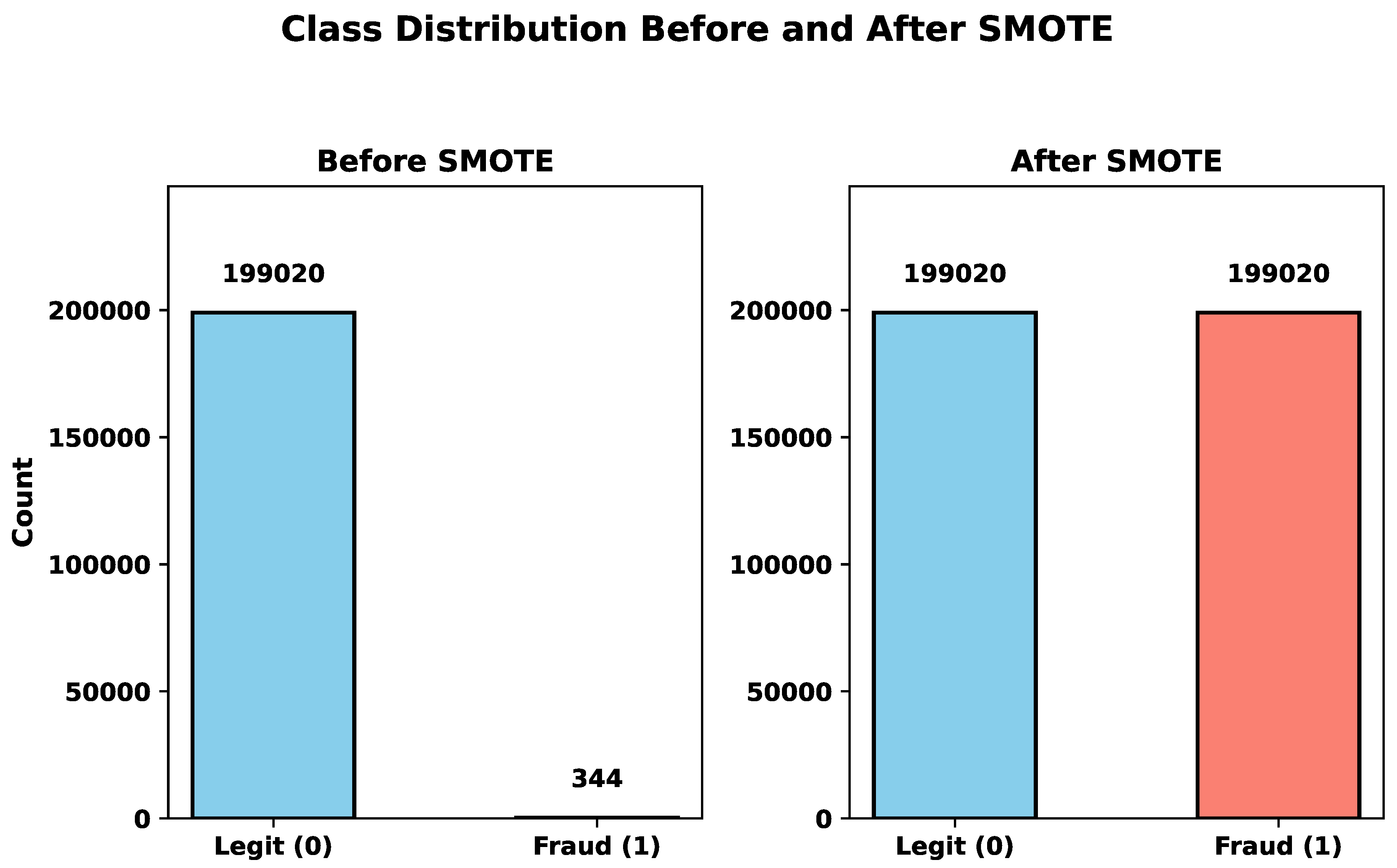
4.1. Data Balancing with SMOTE
The original dataset suffered from a significant class imbalance, as the fraudulent transactions are very rare. This imbalance can negatively impact the model’s ability to learn fraud patterns and make accurate predictions. To address this, the Synthetic Minority Oversampling Technique (SMOTE) was applied to oversample the minority class in the training dataset.
Figure 4.
Comparison of model performance before and after applying SMOTE to handle class imbalance.
Figure 4.
Comparison of model performance before and after applying SMOTE to handle class imbalance.
4.2. Random Forest Evaluation Results
To evaluate the effectiveness of the Random Forest classifier for credit card fraud detection, several standard performance metrics were used, including Accuracy, Precision, Recall, F1 Score, and ROC AUC. These metrics offer insight into the model’s ability to correctly identify fraudulent transactions.
The results in Table 2 show that the model achieved a very high accuracy of 99.95%, indicating strong overall performance. However, due to the imbalanced nature of the dataset, further analysis is provided in Table 3, which details the per-class metrics. The model achieved a precision of 88.06% and a recall of 79.73% for fraud detection, which highlights its capability to detect most fraudulent cases with relatively low false positives.
4.2.1. Confusion Matrix for Random Forest
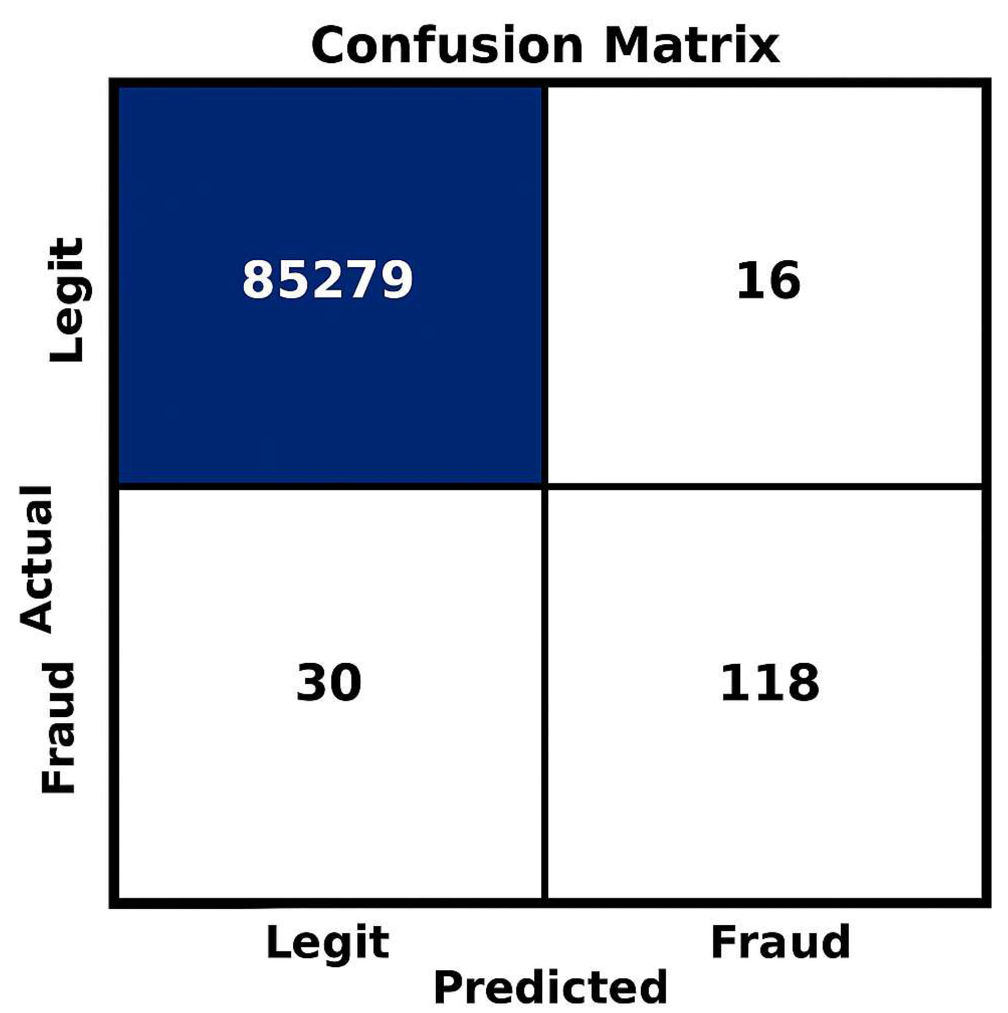
The confusion matrix provides a detailed explanation of the classification results produced by the Random Forest model. It summarizes the number of correct and incorrect predictions made by the model compared to the actual results. The matrix shows 85,279 correctly classified legitimate transactions (true negatives) and 118 correctly identified fraud cases (true positives), with 16 false positives and 30 false negatives. The result of the matrix helps in understanding the working of RF and how efficiently it can differentiate between legitimate and fraudulent transactions.
Figure 5.
Confusion matrix demonstrating the performance of the Random Forest classifier on fraud detection.
Figure 5.
Confusion matrix demonstrating the performance of the Random Forest classifier on fraud detection.
4.2.2. Evaluation Metrics of Random Forest
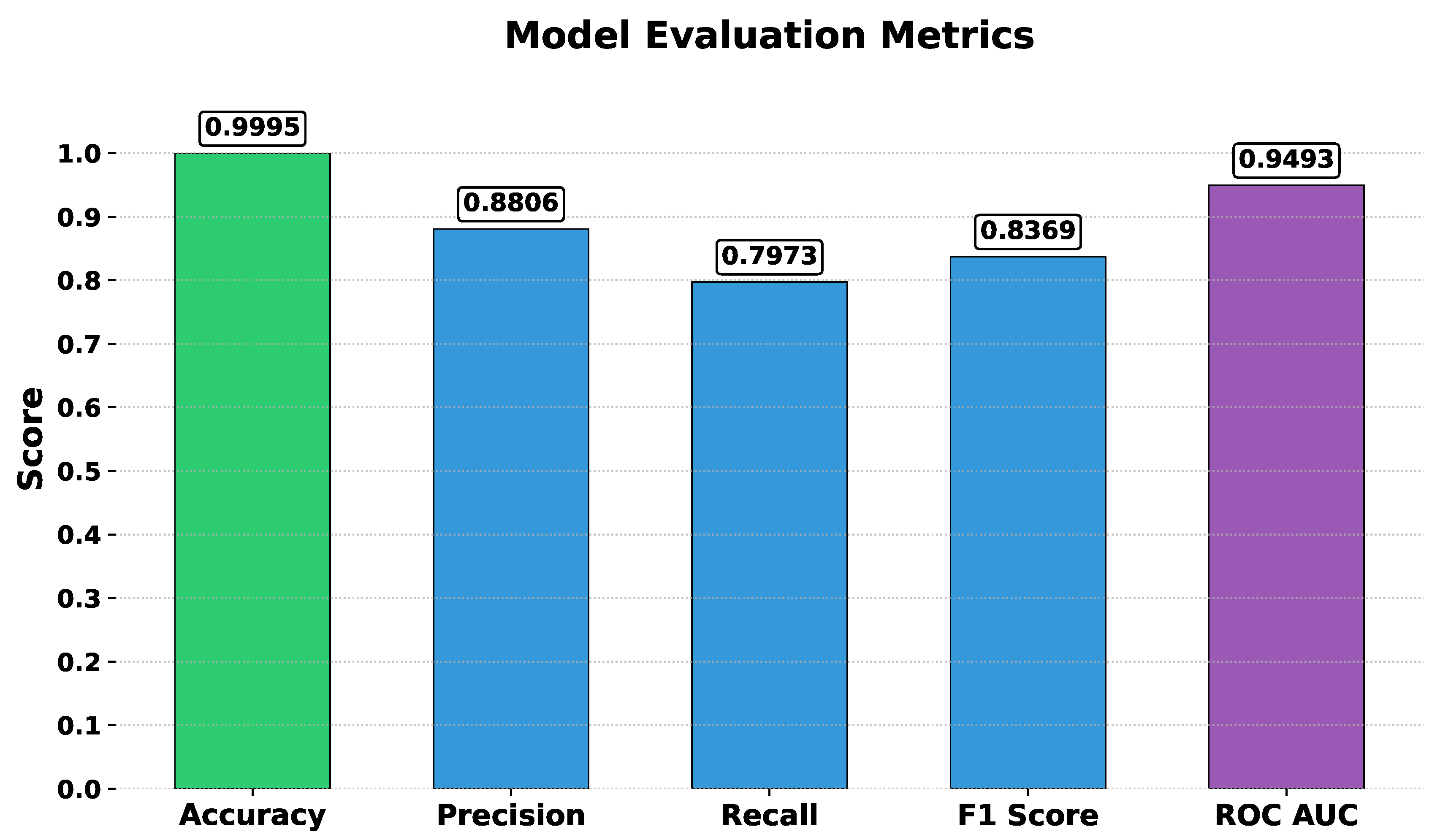
The performance of the Random Forest model was evaluated using several standard classification metrics. The model achieved an accuracy of 0.9994, indicating that it correctly classified nearly all instances in the test set. Precision was 0.8451. This suggests that when the model predicted fraud, it was correct approximately 85% of the time. The recall was 0.8108, meaning that the model correctly identified about 81% of all fraud instances. The F1 score was 0.8276, showing that the model performed well in terms of both false positives and false negatives, and the ROC AUC score was 0.9775, indicating a high ability of the model to discriminate between legitimate and fraudulent transactions. These metrics demonstrate that the Random Forest model performs efficiently in detecting fraud in financial transactions, with a high degree of accuracy and reliability.
Figure 6.
Evaluation Metrics Result of Random Forest
4.2.3. ROC Curve for Random Forest
The ROC curve helps to evaluate how well Random Forest differentiates between fraudulent and legitimate transactions across different thresholds. The models achieved 0.9493 of the curve rate.
Figure 7.
Receiver Operating Characteristic (ROC) curve for the Random Forest classifier

4.2.4. LIME Explanation for Random Forest
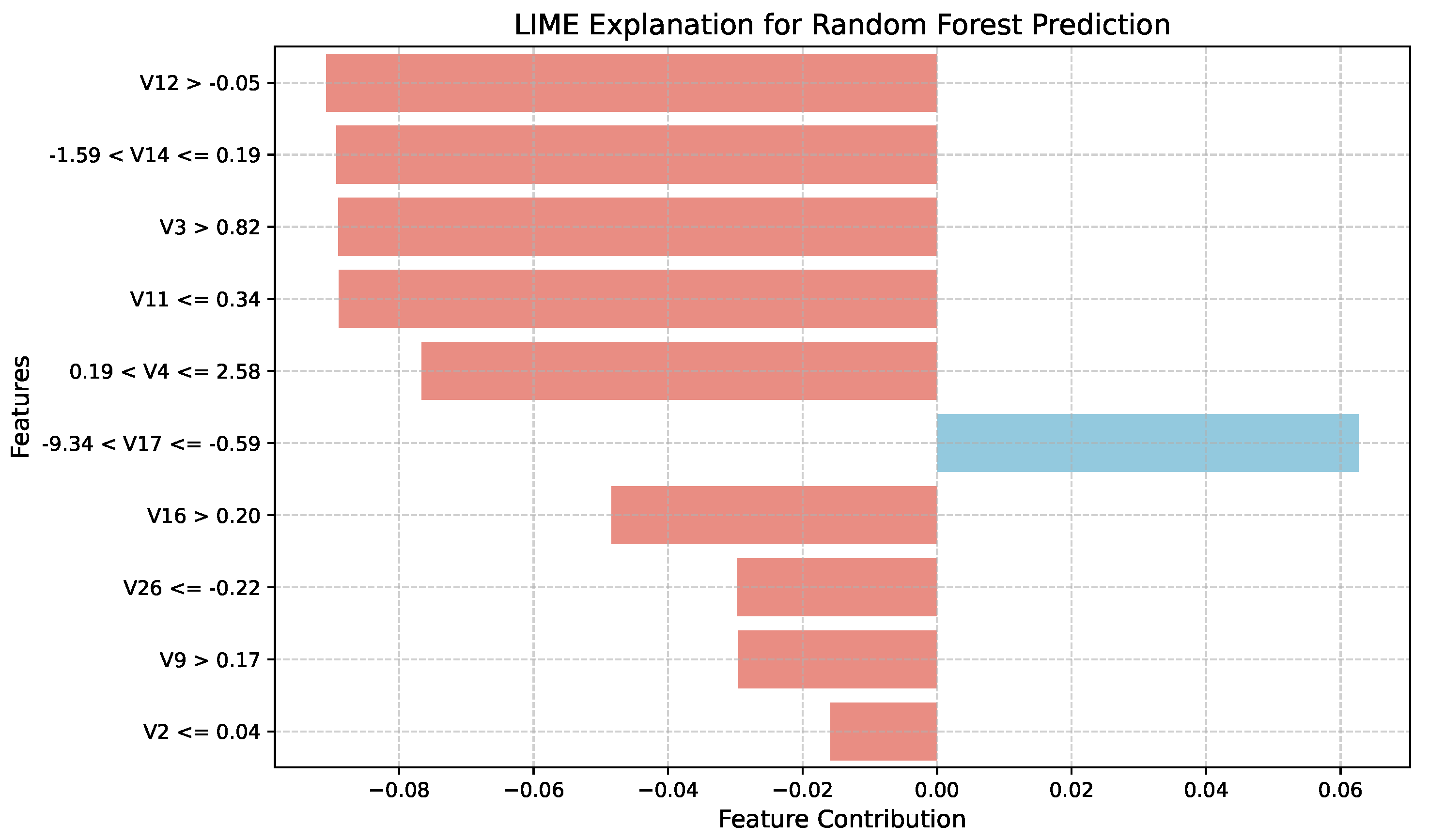
LIME was applied to enhance the interpretability of Random Forest. The LIME explanation revealed the most influential features and their contributions to the prediction probability. The model predicted the instance as legitimate with a probability of 1.00. Among the top contributing features were V4 , V12, V10, and V14, contributing 0.16, 0.12, 0.11, and 0.10 respectively to the prediction of a legitimate transaction. Other features such as V17, V11, and V16 also played minor but notable roles in the model’s decision. This local explanation demonstrates that the Random Forest model bases its decision on a combination of key features, making its predictions interpretable at an instance level.
Figure 8.
LIME explanations for Random Forest predictions
4.3. SHAP Analysis for Random Forest
To interpret the Random Forest model’s predictions, SHAP was applied to the final prediction of the model. The explainer was trained on the resampled training data to account for class imbalance. Features are ranked by importance, with V14 (mean ) and V12 (0.07) having the highest influence on model outputs. Figure 9 shows the global feature importance for fraud (class 1) predictions.
4.4. Results for XGBoost Model
The XGBoost model was trained on the credit card fraud detection dataset. The model was trained on a resampled dataset using SMOTE to handle the class imbalance. As shown in Table 4, the XGBoost model achieved an accuracy of 0.9994, F1 score of 0.8276 indicated a balanced performance between precision and recall, and the ROC AUC score of 0.9775 reflects the model’s strong ability to discriminate between true positives and negatives.
The classification report for the XGBoost model is presented in Table 5, which provides detailed performance metrics including precision, recall, and F1-score for each class (fraud and legitimate transactions):
4.4.1. Evaluation Metrics for XGBoost
The performance of the XGBoost model was evaluated using several evaluation metrics, as shown in Figure 10. The model achieved a high accuracy of 99.94%, precision score was 84.51%, recall was 81.08%, and the F1-score reached 82.76%, reflecting an overall robust fraud detection capability. Additionally, the ROC AUC value of 0.9775 confirms excellent discrimination ability between legitimate and fraudulent transactions. These results indicates that XGBoost is an effective model for credit card fraud detection in imbalanced datasets.
4.4.2. Confusion Matrix for XGBoost
Confusion matrix shown in Figure 11 of the XGBoost classifier for fraud detection, showing 85,273 correctly classified legitimate transactions (true negatives) and 120 accurately detected fraud cases (true positives), with 22 false positives and 28 false negatives. The model achieves a high specificity of 99.97% and recall of 81.08% for the fraud class.
4.4.3. ROC Curve for XGBoost
The Receiver Operating Characteristic (ROC) curve for the XGBoost classifier, illustrated in Figure 12, shows a steep rise towards the top-left corner which indicates that a high true positive rate with a relatively low false positive rate. The Area Under the Curve (AUC) value of approximately 0.9775 highlights the strong discriminative capability of the XGBoost model, making it a reliable choice for fraud detection in imbalanced datasets.
4.4.4. LIME Explanation for XGBoost
To enhance the interpretability of the XGBoost model, Local Interpretable Model-agnostic Explanations (LIME) were employed. The visualization in Figure 13 displays the contribution of each feature to a specific prediction to understand which attributes most influenced the classifier’s decision in that instance.This explainability helps in making decisions to solve real world problems.
4.5. SHAP Explanation for XGBoost
To further interpret the predictions of the XGBoost classifier, SHapley Additive exPlanations (SHAP) were used. Figure 14 shows the SHAP summary plot, which ranks features by their overall importance and displays the impact of feature values on model output. The top features identified include those most influential in distinguishing between fraudulent and non-fraudulent transactions. Additionally, a force plot was generated for a single fraud case to visualize how individual feature values contributed to the prediction. These explanations are valuable for validating model decisions and enhancing transparency in high-stakes financial applications.
5. Comparative Analysis of Random Forest and XGBoost Models
This section presents a comparative analysis of the Random Forest and XGBoost models based on key performance metrics for credit card fraud detection in online transactions. The evaluation focuses on Accuracy, Precision, Recall, F1-score, and ROC AUC.
5.1. Performance Analysis of Random Forest and XGBoost based on Evaluation Metrics
As shown in Table 6, both models achieved high accuracy values above 99.9%, indicating excellent overall performance. However, due to the imbalanced nature of the dataset, other metrics are more indicative of effectiveness in detecting fraud. Random Forest achieved higher precision (0.8806), implying it produced fewer false positives when classifying fraudulent transactions. This can be advantageous in reducing unnecessary investigations triggered by misclassified legitimate transactions. On the other hand, XGBoost yielded a slightly higher recall (0.8108), suggesting it was better at detecting actual fraud cases. This higher sensitivity can be crucial in minimizing the number of fraudulent transactions that go unnoticed.
In terms of the F1-Score, Random Forest slightly outperformed XGBoost (0.8369 vs. 0.8276). However, XGBoost achieved a notably higher ROC AUC (0.9775), reflecting superior capability in distinguishing between the two classes across various thresholds.
5.2. Interpretability Analysis Using SHAP and LIME
To gain deeper insight into how the Random Forest (RF) and XGBoost (XGB) models make fraud predictions, both global (SHAP) and local (LIME) explanation techniques were used. Table 7 summarizes the top features and key findings from each method.
5.2.1. Global Explanations (SHAP)
Both models identify V14, V12, and V4 as their most important predictors of fraud, but XGBoost’s SHAP values are an order of magnitude larger, which indicates greater confidence in its predictions. Unlike Random Forest, where Time is nearly negligible, XGBoost ranks Time fifth, suggesting it captures temporal patterns missed by RF. Furthermore, XGBoost’s sharper drop-off after the top features and the prominence of V26 highlight its sensitivity to a smaller set of highly predictive variables.
5.2.2. Local Explanations (LIME)
Both models flag V4 , V12 > 0.17, and V14 as strong fraud indicators. However, XGBoost uncovers additional nuanced conditions—such as V8 , V22 , and narrow ranges of V15—which are absent in the RF explanations. This suggests XGBoost can detect more subtle patterns, whereas RF provides more conservative and robust thresholds.
5.2.3. Comparative Insights
- Feature Focus: Both models rely on the same core features (V14, V12, V4), but XGBoost’s more extreme SHAP values imply stronger reliance and higher prediction confidence.
- Temporal Dynamics: XGBoost leverages Time significantly, which indicates its ability to exploit time-based fraud patterns, whereas RF largely ignores this feature.
- Pattern Complexity: XGBoost identifies additional feature interactions and precise value ranges (e.g., V8, V22, V15), highlighting its superior capacity to model complex relationships.
- Robustness vs. Sensitivity: Random Forest offers robust and interpretable thresholds that may generalize better, while XGBoost provides more sensitive, but potentially over-specialized patterns.
6. Discussion
The presented study implemented two machine learning models, Random Forest and XGBoost, on the European credit card fraud dataset for detecting fraud in online transactions. To address the major gap, interpretability, and explainability, two XAI tools, SHAP and LIME, were also employed on the final predictions of the models. The main goal of this study was to implement both models to not just evaluate their performance in detecting fraud but also to check which model explains its decisions best so that the better model could be selected in real life. The results show that while Random Forest offered slightly higher precision and clearer interpretability, XGBoost achieved better recall and ROC AUC, making it more effective in identifying fraudulent transactions. Interpretability analysis revealed that both models consistently highlight V4, V12, and V14 as critical fraud indicators. However, XGBoost captured more temporal and complex patterns, whereas Random Forest provided simpler, more robust thresholds. Practically, Random Forest suits in scenarios where precision and not detailed interpretability are important, while XGBoost is preferable when recall is critical and deep explanation is needed. An ensemble approach can balance their strengths. Regular model retraining and monitoring of temporal features like Time are essential to maintain detection effectiveness.
Overall, combining performance and interpretability insights enables the deployment of reliable, transparent, and business-aligned fraud detection systems.The Table 8 contains the results achieved in this study.
7. Conclusions
The study presented a comparative analysis of Random Forest and XGBoost models for credit card fraud detection. The results show that Random Forest achieves slightly higher precision, while XGBoost performs better in terms of recall and ROC AUC. The interpretability analysis using SHAP and LIME provided insights into the most influential features, helping to understand model decisions and enhancing trust in real-world deployment. In interpretability, XGB performs better than RF. Overall, both models demonstrate strong performance in identifying fraudulent transactions, and the study highlights the importance of combining predictive accuracy with interpretability in financial applications. While this study demonstrates the effectiveness of Random Forest and XGBoost models for credit card fraud detection, there are several possibilities for improvement available too for the future as hybrid approach could be explored, Exploring more advanced explainability techniques, Integrating these models into a real-time fraud detection system, and To assess the generalizability of the models, it would be valuable to test the Random Forest and XGBoost models on a wider variety of fraud detection datasets.
Acknowledgments
This research is supported by Multimedia University through its article page charge sponsorship scheme.
References
- Tayebi, M.; El Kafhali, S. A Novel Approach based on XGBoost Classifier and Bayesian Optimization for Credit Card Fraud Detection. Cyber Secur. Appl. 2025. [Google Scholar] [CrossRef]
- Yan, X.; Jiang, Y.; Liu, W.; Yi, D.; Wei, J. A Data Balancing and Ensemble Learning Approach for Credit Card Fraud Detection. arXiv 2024, arXiv:2409.14327. [Google Scholar]
- Feng, X.; Kim, S.-K. Novel Machine Learning Based Credit Card Fraud Detection Systems. Mathematics 2024, 12, 1869. [Google Scholar] [CrossRef]
- Ali, A.; Razak, S.A.; Othman, S.H.; Elfadil, T.A.E.; Al-Dhaqm, A.; Nasser, M.; Elhassan, T.; Elshafie, H.; Saif, A. Financial Fraud Detection Based on Machine Learning: A Systematic Literature Review. Applied Sciences 2022, 12, 9637. [Google Scholar] [CrossRef]
- Kalid, S.N.; Khor, K.-C.; Ng, K.-H.; Tong, G.-K. A Systematic Review on Credit Card Fraud and Payment Default Detection: Challenges, Methods, and Future Directions. *IEEE Access* **2024**, *12*, 23636–23658. [CrossRef]
- Aschi, M.; Bonura, S.; Masi, N.; Messina, D.; Profeta, D. Cybersecurity and Fraud Detection in Financial Transactions. In *Lecture Notes in Computer Science*; Springer: Cham, Switzerland, 2022; pp. 269–278. [Google Scholar]
- Smith, J.; Zhang, R.; Kumar, L. A Novel Ensemble Belief Rule-Based Model for Online Payment Fraud Detection. *Appl. Sci.* **2025**, *15*(3), 1555.
- Dastidar, P.; Author2, A.; Author3, B. Comprehensive Survey on Machine Learning Methods for Fraud Detection, Highlighting Random Forest and XGBoost as Leading Models. *IEEE Access* **2024**, *12*, 12345–12367.
- Wijaya, M.G.; Pinaringgi, M.F.; Zakiyyah, A.Y. ; Meiliana. Comparative Analysis of Machine Learning Algorithms and Data Balancing Techniques for Credit Card Fraud Detection. *IEEE Access* **2024**, *12*, 12345–12367.
- Kennedy, R.K.L.; Villanustre, F.; Khoshgoftaar, T.M. Unsupervised Feature Selection and Class Labeling for Credit Card Fraud. *Journal of Big Data* **2025**, *12*, 111.
- Hancock, J.T.; Khoshgoftaar, T.M.; Liang, Q. A Problem-Agnostic Approach to Feature Selection and Analysis Using SHAP. *J. Big Data* **2025**, *12*, 1–22.
- Mazori, A.A.; Ayub, N. Online Payment Fraud Detection Model Using Machine Learning Techniques. *IEEE Access* **2023**, *11*.
- Alarfaj, A.; Shahzadi, S. Comparative Analysis of Random Forest and XGBoost Using GNNs. *IEEE Access* **2024**.
- Wu, Y.; Wang, L.; Li, H. A Deep Learning Method of Credit Card Fraud Detection Based on Continuous-Coupled Neural Networks. *Mathematics* **2025**, *13*, 819.
- Imani, M.; Beikmohammadi, A.; Arabnia, H.R. Comprehensive Analysis of Random Forest and XGBoost Performance with SMOTE, ADASYN, and GNUS Under Varying Imbalance Levels. *Technologies* **2025**, *13*, 88.
- Mosa, D.T.; Sorour, S.E. CCFD: Efficient Credit Card Fraud Detection Using Meta-Heuristic Techniques and Machine Learning Algorithms. *Mathematics* **2024**, *12*, 2250.
- Liu, Y.; Zhang, X.; Wang, Z. The information content of financial statement fraud risk: An ensemble learning approach. *Decision Support Systems* **2024**, *182*, 114231.
- Nuruzzaman Nobel, S.M.; Sultana, S.; Jan, T. Unmasking Banking Fraud: Unleashing the Power of Machine Learning and Explainable AI (XAI) on Imbalanced Data. *Information* **2024**, *15*, 298.
- Aljunaid, S.K.; Almheiri, S.J.; Dawood, H.; Khan, M.A. Secure and Transparent Banking: Explainable AI-Driven Federated Learning Model for Financial Fraud Detection. *J. Risk Financ. Manag.* **2025**, *18*, 179.
- Herreros-Martínez, A.; Magdalena-Benedicto, R.; Jan, T. Applied Machine Learning to Anomaly Detection in Enterprise Purchase Processes: A Hybrid Approach Using Clustering and Isolation Forest. *Information* **2025**, *16*.
- Shao, Z.; Ahmad, M.N. Comparison of Random Forest and XGBoost Classifiers Using Integrated Optical and SAR Features for Mapping Urban Impervious Surface. *Remote Sens.* **2024**, *16*, 665.
- Caelen, O. Machine Learning Methods for Credit Card Fraud Detection: A Survey. *IEEE Access* **2024**, *12*.
- Jain, R.; Kumari, S.; Kumar, A.; Singh, P. Comparative Study of Machine Learning Algorithms for Credit Card Fraud Detection. *Mathematics* **2022**, *10*(9), 1480.
- Dichev, A.; Zarkova, S.; Angelov, P. Machine Learning as a Tool for Assessment and Management of Fraud Risk in Banking Transactions. *Journal Name* **2025**, *Volume*(Issue), Page numbers.
- Tursunalieva, A.; Alexander, D.L.J.; Dunne, R.; Li, J.; Riera, L.; Zhao, Y. Making Sense of Machine Learning: A Review of Interpretation Techniques and Their Applications. *Appl. Sci.* **2024**, *14*, 496.
- Btoush, E.; Zhou, X. Achieving Excellence in Cyber Fraud Detection: A Hybrid ML+DL Ensemble Approach for Credit Cards. *Appl. Sci.* **2025**, *15*, 10816.
- Khalid, A.R.; Owoh, N.; Uthmani, O.; Ashawa, M.; Osamor, J.; Adejoh, J. Enhancing Credit Card Fraud Detection: An Ensemble Machine Learning Approach. *Big Data Cogn. Comput.* **2024**, *8*, 6.
Figure 9.
SHAP (SHapley Additive exPlanations) summary plot for the Random Forest model
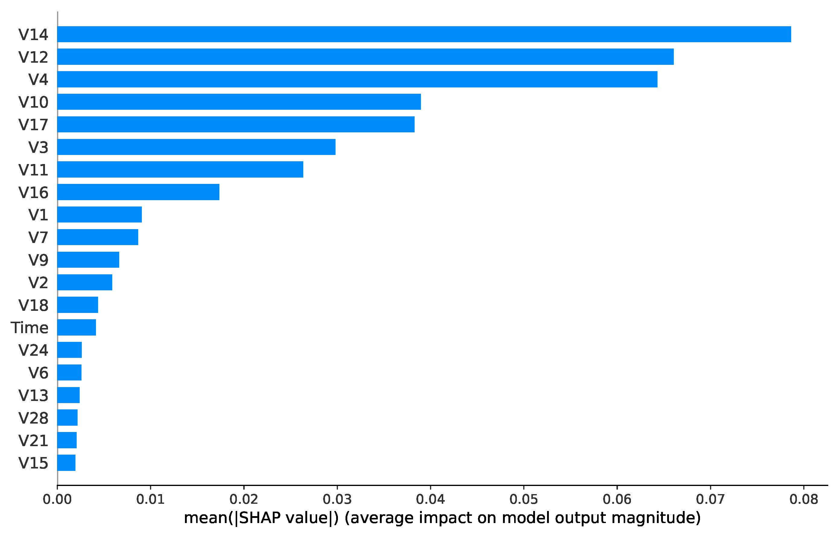
Figure 10.
Evaluation Metric Results of XGBoost

Figure 11.
Confusion Matrix of XGBoost
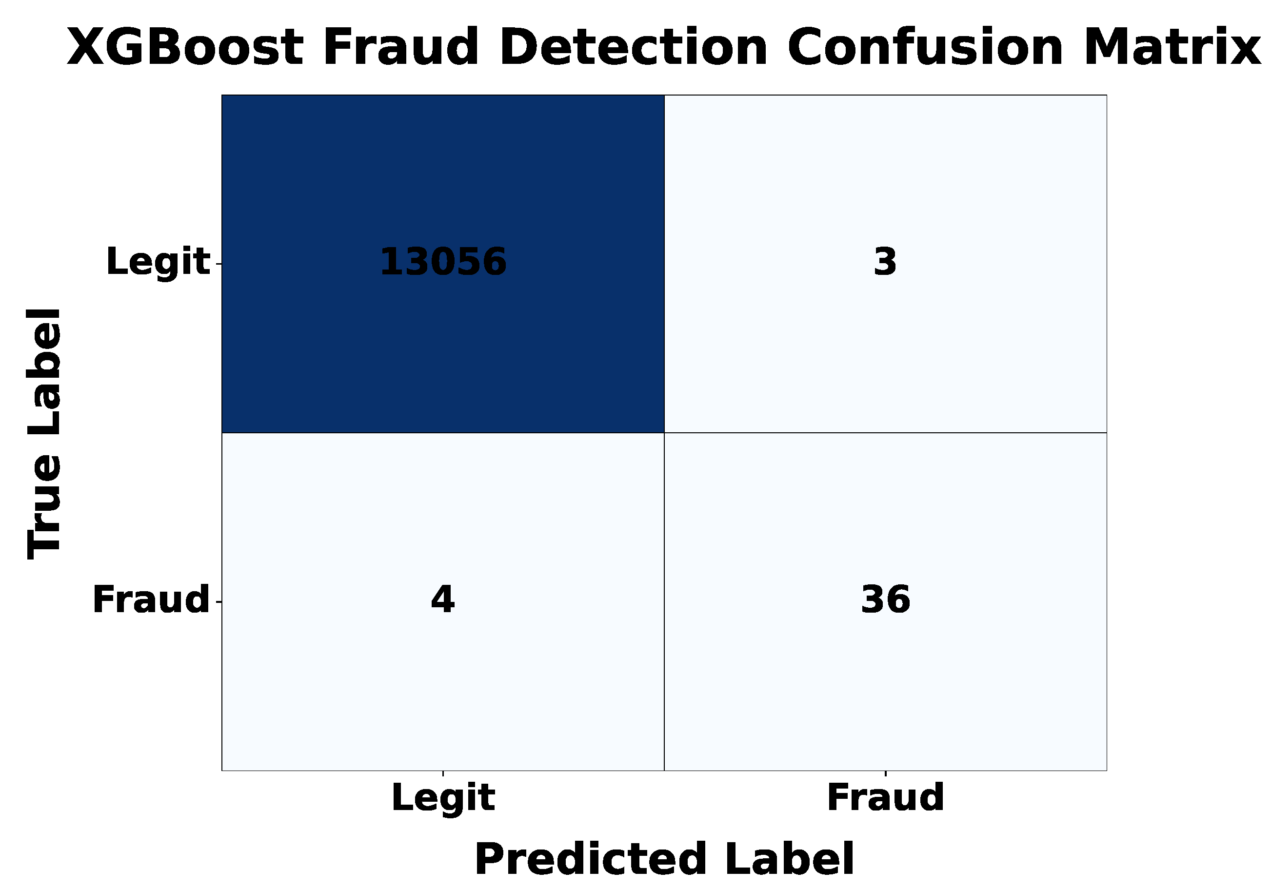
Figure 12.
ROC-AUC Curve of XGBoost
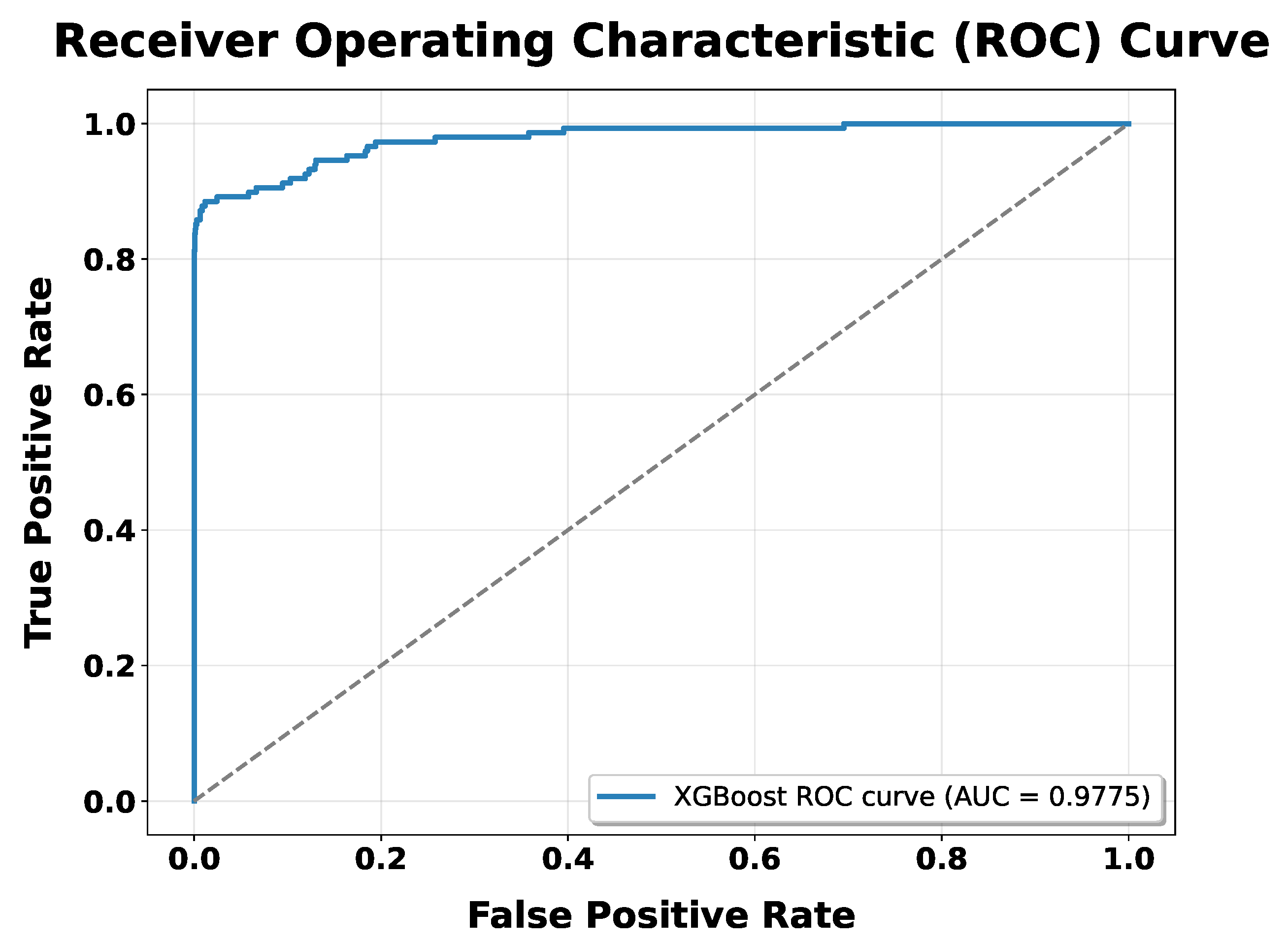
Figure 13.
LIME Explanation for XGBoost
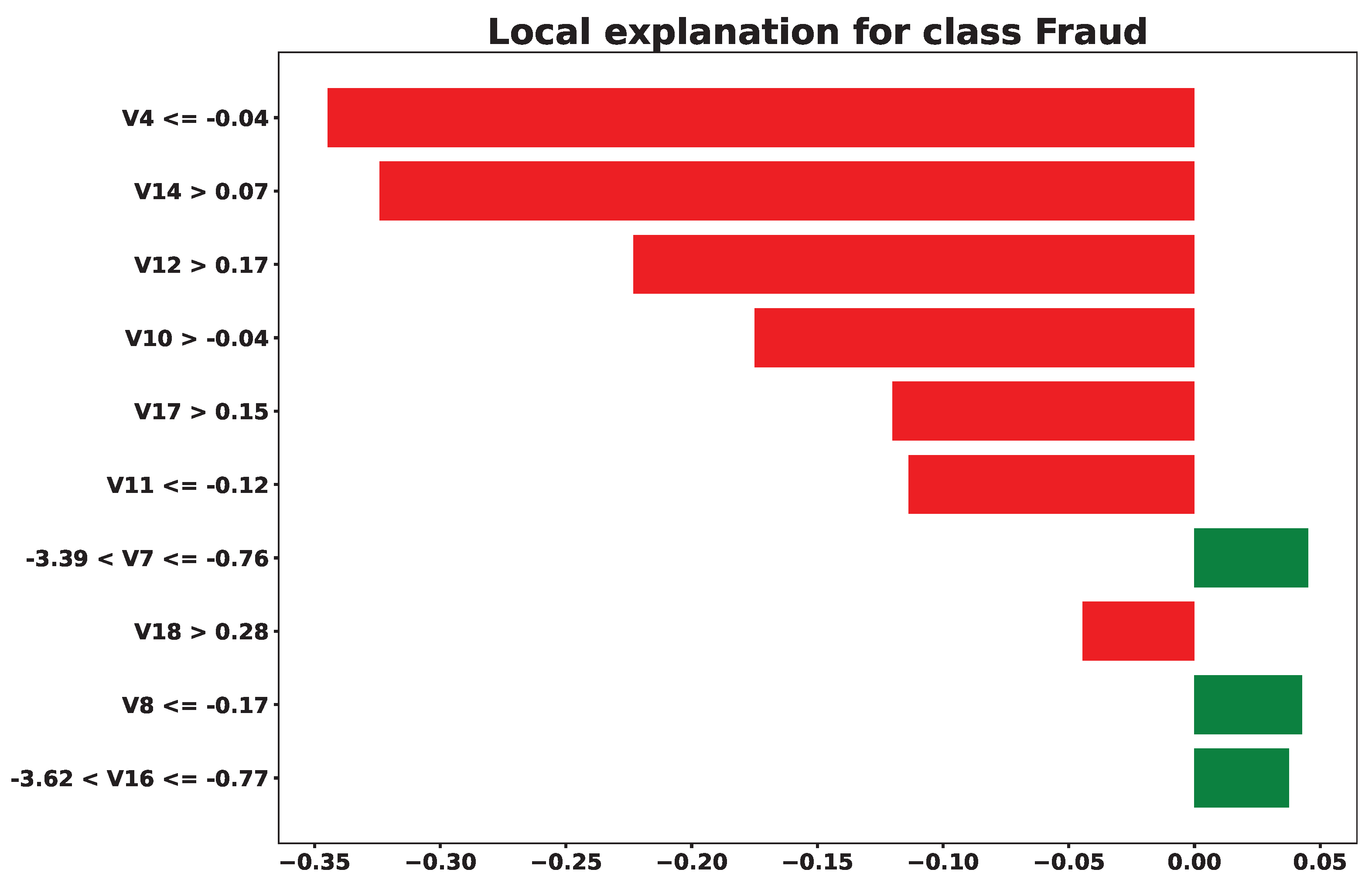
Figure 14.
SHAP Explanation for XGBoost
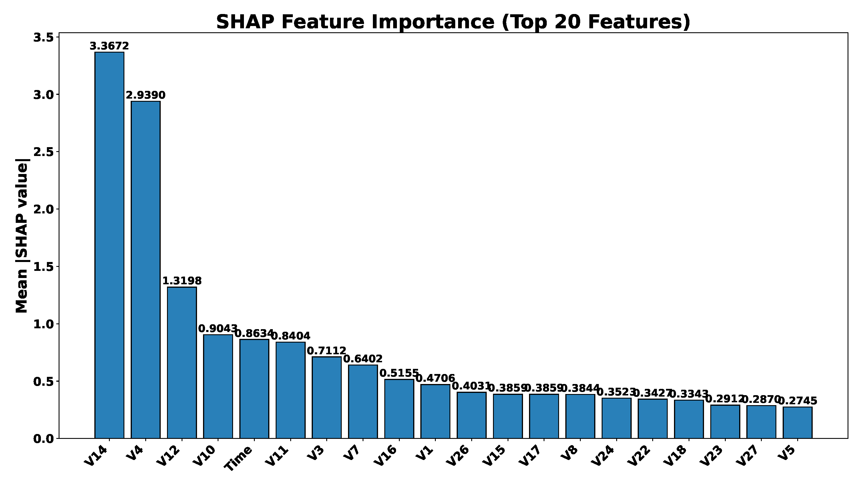
Table 2.
Evaluation metrics of Random Forest for credit card fraud detection.
| Metric | Value |
|---|---|
| Accuracy | 0.9995 |
| Precision | 0.8806 |
| Recall | 0.7973 |
| F1 Score | 0.8369 |
| ROC AUC | 0.9493 |
Table 3.
Classification report of Random Forest.
| Class | Precision | Recall | F1-score | Support |
|---|---|---|---|---|
| 0 (Legit) | 1.00 | 1.00 | 1.00 | 85,295 |
| 1 (Fraud) | 0.88 | 0.80 | 0.84 | 148 |
| Accuracy | 1.00 (on 85,443 instances) | |||
| Macro Avg | 0.94 | 0.90 | 0.92 | 85,443 |
| Weighted Avg | 1.00 | 1.00 | 1.00 | 85,443 |
Table 4.
XGBoost Model Evaluation Metrics
| Metric | Score |
|---|---|
| Accuracy | 0.9994 |
| Precision | 0.8451 |
| Recall | 0.8108 |
| F1 Score | 0.8276 |
| ROC AUC | 0.9775 |
Table 5.
XGBoost Model Classification Report
| Class | Precision | Recall | F1-Score |
|---|---|---|---|
| 0 | 1.00 | 1.00 | 1.00 |
| 1 | 0.85 | 0.81 | 0.83 |
| Accuracy: 0.9994 | |||
| Macro Avg | 0.92 | 0.91 | 0.91 |
| Weighted Avg | 1.00 | 1.00 | 1.00 |
Table 6.
Performance Comparison of Random Forest and XGBoost.
| Metric | Random Forest | XGBoost |
|---|---|---|
| Accuracy | 0.9995 | 0.9994 |
| Precision | 0.8806 | 0.8451 |
| Recall | 0.7973 | 0.8108 |
| F1-Score | 0.8369 | 0.8276 |
| ROC AUC | 0.9493 | 0.9775 |
Table 7.
Key Interpretability Results for RF and XGB Models
| Aspect | Random Forest | XGBoost |
|---|---|---|
| Top SHAP Features | V14, V12, V4 (0.07–0.08)V10, V17, V3, V11, V16 (0.03–0.06) | V14, V4, V12 (2.5–3.5)V10, Time, V11, V3 (1.0–2.0)V7, V16, V1, V26 (0.5–1.0) |
| SHAP Insights | Focus on 8–10 features;Time not important | Stronger impact;Time ranks 5th; V26 important |
| Top LIME Indicators | V4 (+0.16);V12 > 0.17 (+0.13);V10 > -0.04 (+0.11);V14 > 0.07 (+0.10);V17 > 0.15 (+0.09) | V4 ;V14 > 0.07;V12 > 0.17;V10 > -0.04;V11 ;V17 > 0.15 |
| Additional LIME Patterns | V16 (-3.62 to -0.77);V7 (-3.39 to -0.76) | V7 (-3.39 to -0.76);V8 ;V22 ;V15 (-0.02 to 0.57) |
| Model Sensitivity | Focused and robust;clear thresholds | More extreme;sensitive to additional features |
Table 8.
Comparison Between Random Forest and XGBoost.
| Category | Metric | Random Forest | XGBoost | Winner |
|---|---|---|---|---|
| Performance | Accuracy | 0.9995 | 0.9994 | RF |
| Precision | 0.8806 | 0.8451 | RF | |
| Recall | 0.7973 | 0.8108 | XGB | |
| F1 Score | 0.8369 | 0.8276 | RF | |
| ROC AUC | 0.9493 | 0.9775 | XGB | |
| Interpretability | SHAP Focus | Spread out features | V14, V4, V12 dominant | XGB |
| LIME Clarity | Less threshold info | Clear (V14 > 0.07, V4 ≤ -0.04) | XGB | |
| Imbalance | SHAP Shift Stability | Small changes | Large jump (+14.59) | XGB |
| Efficiency | Training Speed | Slower (bagging) | Faster (boosting) | XGB |
Disclaimer/Publisher’s Note: The statements, opinions and data contained in all publications are solely those of the individual author(s) and contributor(s) and not of MDPI and/or the editor(s). MDPI and/or the editor(s) disclaim responsibility for any injury to people or property resulting from any ideas, methods, instructions or products referred to in the content. |
© 2025 by the authors. Licensee MDPI, Basel, Switzerland. This article is an open access article distributed under the terms and conditions of the Creative Commons Attribution (CC BY) license (http://creativecommons.org/licenses/by/4.0/).
Copyright: This open access article is published under a Creative Commons CC BY 4.0 license, which permit the free download, distribution, and reuse, provided that the author and preprint are cited in any reuse.


