

Submitted:
11 September 2025
Posted:
12 September 2025
You are already at the latest version
Abstract
Receiver operating characteristic (ROC) surfaces provide a natural extension of ROC curves to three-class diagnostic problems. A key summary index is the volume under the surface (VUS), representing the probability that a randomly chosen observation from each of the three ordered groups is correctly classified. Parametric estimation of VUS typically assumes trinormality of the class distributions. However, a formal method for the verification of this composite assumption has not appeared in the literature. Our approach generalizes the two-class AUC-based GOF test of Zou et al. to the three-class setting by exploiting the parallel structure between empirical and trinormal VUS estimators. We propose a global goodness-of-fit (GOF) test for trinormal ROC models based on the difference between empirical and trinormal parametric estimates of the VUS. To improve stability, a probit transformation is applied and a bootstrap procedure is used to estimate the variance of the difference. The resulting test provides a formal diagnostic for assessing adequacy of trinormal ROC modeling. Simulation studies illustrate the robustness of the assumption via empirical size and power of the test under various distributional settings, including skewed and multimodal alternatives. An application to Covid-19 antibody levels data demonstrates the practical utility of the method. Our findings suggest that the proposed GOF test is simple to implement, computationally feasible for moderate sample sizes, and a useful complement to existing ROC surface methodology.
Keywords:
ROC surface
; VUS
; trinormal model
; goodness-of-fit test
; bootstrap
; Box–Cox transformation
1. Introduction
Receiver operating characteristic (ROC) analysis is a cornerstone of diagnostic test evaluation. While the two-class ROC curve and its area under the curve (AUC) are extensively studied, many clinical problems involve three or more diagnostic categories. The ROC surface generalizes the ROC curve to the three-class setting, and its summary statistic, the volume under the surface (VUS), extends the AUC [1].
A common modeling framework is the trinormal model, which assumes that test results from the three groups (e.g., healthy, intermediate, diseased) are independent normals with increasing means, or that they can be transformed to normality through a common monotone transformation [2]. In practice, the latter assumption is often overlooked: researchers may typically verify only marginal normality within each group. Yet departures from normality for the independent groups do not necessarily invalidate the trinormal assumption as already known from the ROC curve framework [3], while it is reasonable to hypothesize that significant departures such as skewness, heavy tails, or multimodality can invalidate the trinormal model, bias VUS estimation, and undermine inference. Despite this vague reality, formal assessment of the model’s adequacy has received little inadequate attention in the literature.
In the two-class case, Zou et al. [4] developed a large-sample goodness-of-fit (GOF) test for binormal (and bi-Weibull) ROC models. Their method compares a nonparametric AUC estimator with its model-based counterpart, applying a variance-stabilizing transformation (e.g., probit or logit) to enable valid asymptotics. The appeal of this approach is its interpretability: if the parametric model is correct, the two estimates agree up to sampling error; otherwise, their discrepancy reflects lack of fit.
No analogous GOF procedure has been available for ROC surfaces. Yet the ingredients are parallel: the VUS admits both a nonparametric U-statistic estimator and a closed-form expression under the trinormal model. This makes possible a natural extension of the Zou et al. framework: compare empirical and trinormal VUS estimates, possibly after transformation, using resampling to calibrate inference.
Such an extension matters because the trinormal model is pervasive in ROC surface analysis, especially for very large samples where nonparametric estimates can be computationally expensive or even infeasible, but real biomedical data may not adhere to trinormality assumptions. The two-class “binormal” framework illustrates the issue: in strict form it posits independent normals with distinct means and variances; in a broader sense, it assumes existence of a monotone transformation yielding approximate normality, exploiting ROC invariance to monotone changes of scale. Transformation-based methods (e.g., Box–Cox with a common exponent) formalize this broader view, yet without a GOF check, adequacy remains unverified.
By importing the GOF philosophy to the three-class setting, we provide a practical diagnostic for trinormal ROC models. Contrasting empirical and parametric VUS estimates highlights when parametric summaries are reliable and when departures from trinormality call for alternative modeling. This brings needed transparency to the routine use of ROC surface methods in practice.
2. Methods
2.1. The Two-Class, Binormal ROC Curve Framework
In the two-class case, receiver operating characteristic (ROC) analysis evaluates the ability of a continuous marker X to distinguish between a non-diseased group () and a diseased group (). Under the binormal model, we assume
with independent samples, possibly after a common transformation to normality that will allow for efficient use of the model. The ROC curve can then be written in closed form as
where is the standard normal distribution function and t is the false positive rate (FPR). The area under the curve (AUC), which summarizes overall discriminatory ability, has the simple expression:
This form highlights that, in the binormal setting, the AUC depends only on the standardized mean difference between groups. Equivalently, the AUC can be interpreted as the probability that a randomly chosen diseased subject will have a higher marker value than a randomly chosen non-diseased subject.
2.2. Box–Cox for Binormal ROC
A pragmatic route to approximate binormality for continuous diagnostic markers is to apply a common monotone power transformation across groups prior to model fitting [5]. Let,
and suppose and are approximately normal with distinct means/variances for a single shared by both classes. Because the ROC curve is invariant to monotone transformations, estimation and inference can proceed on the transformed scale while reporting cutoffs back on the original scale. A comprehensive binormal workflow based on this idea, including point and interval estimation for AUC, the maximized Youden index, its cutoff and joint inference, as well as two-marker comparisons, has been developed by Bantis et al. [6] and implemented in the rocbc package, with procedures that account for the uncertainty in and tools to check whether a Box–Cox transformation can plausibly achieve approximate normality [7,8,9].
In practice is estimated (e.g., by profile likelihood under normality on ). This yields semi-parametric robustness (via transformation) without abandoning the interpretability and efficiency of binormal ROC when the transformed model is adequate.
2.3. Goodness-of-Fit Testing in the Binormal Framework
To formally assess the binormal assumption in ROC curve analysis, Zou et al. [4] proposed a global goodness-of-fit test based on comparing non-parametric and parametric estimates of the area under the curve (AUC). The non-parametric AUC is given by
where and denote test results from the non-diseased and diseased samples, respectively. Under the binormal model, and , the parametric AUC is,
with the standard normal distribution function [13]. Since AUC values are confined to , both and are stabilized via the probit transform, . The test statistic is then constructed as,
where the standard error in the denominator is estimated by a stratified bootstrap resampling of the diseased and non-diseased groups. Under the null hypothesis that the binormal model is correct, is asymptotically standard normal, and the two-sided p-value is .
2.4. The Three-Class, ROC Surface Framework
Let , , and denote independent test results from healthy, intermediate, and diseased populations with cumulative distributions , respectively. The VUS is defined as It represents the probability that the diagnostic marker correctly orders a randomly selected triple. The nonparametric estimator of VUS is a U-statistic:
where are class sample sizes. This estimator is unbiased but computationally intensive for large n [10].
Under the trinormal model, , , . The trinormal ROC surface and corresponding VUS have closed-form expressions [11].
The closed-form expression for VUS is derived as follows. Let,
Denote by the standard bivariate normal CDF with correlation ,
Then, under the trinormal model,
For the equivalent form pertinent to the four-parameter trinormal ROC surface model, define
Then
and hence,
The VUS is estimated by maximum likelihood fitting of the class-specific normals. We denote this estimator by . These expressions follow the standard trinormal ROC parameterization reviewed in Noll et al. [2].
2.5. Box–Cox for Trinormal ROC Surfaces
The Box–Cox ROC curve framework extends to three-class ROC surface analysis by applying a common Box–Cox transformation to all three groups, then fit a trinormal model to and compute VUS on the transformed scale. Methodology and software exist for this pathway: trinROC includes boxcoxROC for automatic selection of a common and transformed-scale fitting, while earlier work by Bantis, Nakas and Reiser developed joint inference for the optimal true-class fractions of ROC surfaces using Box–Cox as a parametric backbone [12]. Noll et al. [2] formalized inference and testing for ROC surfaces under the trinormal model, and explicitly connected these procedures with Box–Cox–type transformations.
Transformation-based modeling does not obviate the need to verify the trinormal working model. Even with good empirical performance, adequacy should be tested rather than assumed. In the two-class case, goodness-of-fit testing compares a nonparametric AUC to its model-based counterpart after variance-stabilizing transformation; an analogous comparison for VUS provides a principled diagnostic for trinormal ROC surfaces. Embedding a Box–Cox pre-processing step and a subsequent GOF test adds essential formalism to the routine use of binormal/trinormal ROC models, clarifying when parametric summaries are trustworthy and when departures from trinormality warrant alternatives [6].
2.6. Proposed Trinormal GOF Test
Extending the two-class framework [4], we compare the empirical and parametric trinormal VUS estimates. Because VUS , we apply a probit transformation, , where is the standard normal quantile function. Define, . We estimate by bootstrap resampling (resampling within each class). The test statistic is
which is asymptotically under the null hypothesis that the trinormal model is valid. Large values of D indicate lack of fit, with two-sided p-values obtained accordingly.
The procedure was implemented in R, using the trinROC package for empirical and trinormal VUS estimation, and boxcoxROC for optional transformation to normality. We provide the code in Appendix A.
3. Simulation Scenarios and Results
To assess the impact of distributional assumptions and potential deviations from trinormality on the estimation of VUS, we conducted a series of simulation experiments under nine distinct data-generating scenarios (A–I), reviewed in Table 1 and illustrated visually in Figure 1. For each setting, independent samples of size 2000 were drawn from distributions assigned to the three diagnostic groups, denoted . Increments in means across groups were maintained to enforce an ordering of disease severity. . Each scenario was constructed to represent common or challenging situations encountered in diagnostic test evaluation, ranging from symmetric Gaussian distributions with increasing means, to skewed lognormal or gamma settings, to mixture models and heavy-tailed distributions.
- Scenarios A–C: Skewed and/or mixture distributions. Scenario A combines a gamma distribution for , a two-component normal mixture for , and a shifted normal for , yielding a high empirical VUS around 0.82. Scenario B introduces a lognormal distribution for , a mixture distribution for , and a chi-square plus normal noise for , producing moderate discrimination (empirical VUS ). Scenario C adopts gamma distributions with increasing shape/scale parameters across groups, targeting a VUS of 0.60. At the same time, these are scenarios where the Box–Cox transformation (or the simpler log one) are expected to fail transforming to normality. The proposed GOF test is expected to exhibit some power to reject the trinormal hypothesis even at low to moderate sample sizes.
- Scenarios D–F: Trinormal benchmarks with equal or unequal variances. Scenario D sets means equally spaced at 0, 0.9, and 1.8 with equal unit variance, while Scenarios E and F gradually increase variance heterogeneity across groups, yielding empirical VUS values close to the 0.50 null benchmark. For these scenarios, even the simple log transformation is expected to perform rather well transforming to normality, with the Box–Cox providing optimal results. The test is expected to approximate the nominal size of used throughout.
- Scenarios G–I: Strong departures from normality. Scenario G uses lognormal distributions with scaling factors, leading to pronounced skewness and low empirical VUS (). Scenario H further exaggerates skewness by shifting the lognormal parameters, targeting VUS . Finally, Scenario I combines a lognormal , a normal mixture , and a highly skewed gamma plus normal noise , resulting in the lowest discrimination (VUS ). Naive estimation of VUS based on a trinormal assumption is expected to fail, while the Box–Cox should show robustness and a valid option towards the use of parametric assumptions.
The diversity of scenarios ensures that both mild and extreme violations of the trinormal assumption are represented, allowing us to evaluate robustness across a wide range of practical conditions. For each scenario, the empirical VUS was estimated via Equation 7. We approximated using averages of Monte Carlo replicates. The naive trinormal plug-in VUS was obtained by estimating group means and variances via maximum likelihood under the normal model and applying the trinormal VUS formula of Equation 10. Similarly, the trinormal plug-in VUS was obtained after each transformation used (log and Box–Cox).
Initially, the focus was on the differences between the empirical VUS and the naive trinormal estimate. The proposed GOF test should reject when departures are high. The scenarios span a wide range of complexities:
- In Scenarios A–F, the empirical and naive trinormal VUS values are broadly consistent, with differences typically below 0.02. For example, Scenario A yields an empirical VUS of 0.818 and a naive VUS of 0.811, while Scenario D (trinormal null) shows 0.504 vs. 0.511. This suggests that moderate skewness or variance heterogeneity does not strongly bias parametric estimates when sample sizes are large.
- Scenarios G–I demonstrate severe discrepancies. In Scenario G, the empirical VUS is 0.295, but the naive trinormal estimate drops to 0.209, substantially underestimating diagnostic performance. In Scenario H, the empirical VUS is 0.699, yet the naive trinormal VUS falls to 0.427, a striking underestimation. Conversely, in Scenario I, the naive estimate (0.602) vastly overstates the empirical VUS (0.214). These results indicate that naive normal modeling can misrepresent discrimination strength, either attenuating or inflating it, when strong departures from normality or mixture structures are present.
Full assessment of the proposed GOF test was conducted via the comparison of the empirical VUS, estimated nonparametrically against, in turn, the naive trinormal plug-in VUS, obtained by fitting normal distributions to each class regardless of the underlying state, the trinormal plug-in VUS estimate after using a simple log transformation, and the trinormal plug-in VUS estimate after using the Box–Cox as an optimal tool for transforming to normality for continuous diagnostic test results in the ROC framework. The goal was to also assess the utility of simple log transformations and the Box–Cox when the naive VUS estimator fails.
- For scenarios A–C, when the naive trinormal VUS estimate is close to the empirical, no transformation appears to be needed regardless of underlying distributions. Transformations may even distort the true underlying discrimination patterns. A fact which is apparent as the sample size grows larger.
- For scenarios D–F, even if underlying distributions are in fact normal, the naive trinormal VUS estimator will fail if significant scale differences exist between the underlying actually normal distribution. This is a very important finding, given that underlying independent normality of the distributions of the three classes does not ensure accurate estimation of the VUS using the naive trinormal model. Even a simple log transformation will provide the needed normalization to trinormality allowing for the use of the parametric VUS model.
- For scenarios G–I, the Box–Cox behaves very well for moderate sample sizes when differences between empirical and naive trinormal VUS estimates are within the range of (scenario G, underlying lognormal distributions), while the simple log transformation does not provide an adequately accurate result. The proposed GOF test exhibits high power in detecting departures from the trinormal model (especially for scenarios H and I). Even when the underlying distributions are lognormal both transformation choices offer little help. In such cases, resorting to nonparametric methods is recommended.
In sum, our simulation study demonstrates that naive trinormal VUS estimates are robust to mild departures from normality but can be severely misleading in some skewed or mixture scenarios where the empirical estimate diverges significantly from the naive trinormal, or even when significant scale differences exist between underlying normal distributions. This emphasizes the need for approximate transformations to normality (e.g., via Box–Cox, or simple log) in the three-class diagnostic setting where biases can propagate into erroneous clinical inference. The use of nonparametric approaches is recommended for extreme differences of empirical versus naive trinormal VUS estimates.
4. Application: Covid-19 Antibody Data
For the application, we illustrate our methodology using antibody data following the first dose of the BNT162b2 Covid-19 vaccine, as reported by [14]. The original study recruited 425 Greek healthcare workers and measured IgG levels against the SARS-CoV-2 spike protein 14 days post-immunization. Their findings indicated robust immunogenicity, with more than 90% of participants developing detectable antibody responses. Importantly, antibody titres displayed a clear age gradient: levels were highest among younger individuals (20–49 years), declined markedly in the 50–59 age group, and dropped further among participants aged 60 years or older. This pattern makes the dataset particularly suitable for exploring three-class ROC methodology, with the age strata serving as distinct groups.
In our analysis, we restricted attention to the age ranges 40–49, 50–59, and 60–69 years, thereby creating three groups with decreasing antibody concentrations. Figure 3 illustrates histograms and boxplots of the raw and log-transformed measurements, while Figure 4 illustrates the corresponding ROC surface estimates according to the possible models used, through standard output of the trinROC package. Applying our trinormal goodness-of-fit test framework, we examined the adequacy of the trinormal assumption under different transformations. Table 3 summarises the results.The raw data showed clear deviations from normality, and the log-transformation improved model fit but still left some departures. By contrast, the Box–Cox transformation provided the best adherence to trinormality, yielding more stable estimates of the volume under the surface (VUS). This example highlights the practical relevance of transformation choice in ROC surface analysis: while simpler transformations such as the logarithm can mitigate skewness, the more flexible Box–Cox approach can better accommodate the distributional characteristics of immunogenicity data, ultimately leading to more reliable inference.
5. Discussion
It is well known that the binormal ROC curve model exhibits a certain robustness to departures from normality in the underlying group distributions. For example, Hanley [?] noted that binormal ROC analysis can still provide useful summaries even when the marker distributions are skewed or heavy-tailed, provided the deviation from normality is not extreme. Nevertheless, the binormal framework remains a parametric model, and its use implicitly assumes validity of the underlying distributional form. In practice, this assumption is seldom tested in ROC curve analysis, though analogous assumptions are routinely checked in classical inference problems such as the t-test or one-way ANOVA. The same issue carries over to ROC surface analysis, where the trinormal model can be adopted in practice but is not subjected to formal GOF evaluation. While ROC surface methodology has matured substantially, formal consideration of distributional adequacy remains underdeveloped. This gap motivates the development of dedicated GOF procedures for ROC surfaces, ensuring that parametric estimates of diagnostic accuracy are not unduly biased by violations of normality.
We proposed a global GOF test for trinormal ROC surfaces based on comparing empirical and parametric VUS estimates. The test generalizes two-class AUC-based GOF tests [4] to three-class settings. The test maintains correct type I error when trinormality holds and has good power against skewed or multimodal alternatives even for moderate sample sizes. Transformations such as the Box–Cox can markedly improve model adequacy as tested using the proposed GOF framework. Limitations include computational cost of the empirical VUS for large n, though our implementation remains feasible for per group. Extensions to higher-class ROC manifolds represent future work.
The proposed GOF test provides a simple and interpretable way to check trinormal assumptions in ROC surface analysis. It complements parametric modeling by highlighting when results are robust and when alternative approaches may be needed. Such model adequacy tests could become routine practice even for standard methods that rely on parametric assumptions, such as the ANOVA.
Funding
This research received no external funding.
Data Availability Statement
Restrictions apply to the availability of these data. Data were obtained from Dr Kontopoulou [14] and are available from the author upon reasonable request, with the permission of Dr Kontopoulou.
Acknowledgments
During the preparation of this manuscript, the author used ChatGPT 5.0 for the purposes of language polishing, R-code optimization, Table and Figure presentation. The author has completely reviewed and edited the output and takes full responsibility for the content of this publication.
Conflicts of Interest
The author declares no conflicts of interest.
Abbreviations
The following abbreviations are used in this manuscript:
| AUC | Area Under Curve |
| FPR | False Positive Rate |
| GOF | Goodness of Fit |
| ROC | Receiver Operating Characteristic |
| TCF | True Class Fraction |
| TPR | True Positive Rate |
| VUS | Volume Under Surface |
Appendix A. R-Code for the Implementation of the Trinormal ROC Model GOF Test Statistic
| library(trinROC) |
| # probit transform for stability |
| probit_transform <- function(p) { |
| p <- min(max(p, 1e-6), 1 - 1e-6) |
| qnorm(p) |
| } |
| # GOF Test for Trinormal VUS |
| gof_test_trinormal <- function(x, y, z, B = 400, boxcox = FALSE) { |
| lambda_opt <- NULL |
| # ---- Optional Box-Cox transformation ---- |
| if (boxcox) { |
| bc <- boxcoxROC(x, y, z, verbose = FALSE) |
| x <- bc$xbc |
| y <- bc$ybc |
| z <- bc$zbc |
| lambda_opt <- bc$lambda # extract optimal lambda |
| } |
| # ---- 1. Nonparametric empirical VUS ---- |
| np_vus <- emp.vus(x, y, z) |
| WN <- probit_transform(np_vus) |
| # ---- 2. Trinormal parametric VUS ---- |
| trin <- trinVUS.test(x, y, z) |
| par_vus <- as.numeric(trin$estimate) |
| WP <- probit_transform(par_vus) |
| # ---- 3. Difference ---- |
| Delta <- WN - WP |
| # ---- 4. Bootstrap variance of Delta ---- |
| boot_deltas <- replicate(B, { |
| xb <- sample(x, length(x), replace = TRUE) |
| yb <- sample(y, length(y), replace = TRUE) |
| zb <- sample(z, length(z), replace = TRUE) |
| npb <- emp.vus(xb, yb, zb) |
| WNb <- probit_transform(npb) |
| tb <- trinVUS.test(xb, yb, zb) |
| parb <- as.numeric(tb$estimate) |
| WPb <- probit_transform(parb) |
| WNb - WPb |
| }) |
| Var_Delta <- var(boot_deltas, na.rm = TRUE) |
| # ---- 5. Test statistic ---- |
| if (Var_Delta <= 0) { |
| D <- NA |
| p_val <- NA |
| } else { |
| D <- abs(Delta) / sqrt(Var_Delta) |
| p_val <- 2 * (1 - pnorm(abs(D))) |
| } |
| list( |
| VUS_nonparam = np_vus, |
| VUS_trinormal = par_vus, |
| WN = WN, WP = WP, |
| Delta = Delta, |
| Var_Delta = Var_Delta, |
| D = D, p_value = p_val, |
| boxcox_used = boxcox, |
| lambda_opt = lambda_opt # return optimal lambda |
| ) |
| } |
References
- Nakas, C.T.; Bantis, L.E.; Gatsonis, C.A. ROC Analysis for Classification and Prediction in Practice, 1st ed.; Chapman and Hall/CRC: Boca Raton, FL, USA, 2023. [Google Scholar] [CrossRef]
- Noll, S.; Furrer, R.; Reiser, B.; Nakas, C.T. Inference in Receiver Operating Characteristic Surface Analysis via a Trinormal Model-Based Testing Approach. Stat 2019, 8, e249. [Google Scholar] [CrossRef]
- Hanley, J.A. The robustness of the “binormal” assumptions used in fitting ROC curves. Med. Decis. Making 1988, 8, 197–203. [Google Scholar] [CrossRef] [PubMed]
- Zou, K.H.; Resnic, F.S.; Talos, I.F.; Goldberg-Zimring, D.; Bhagwat, J.G.; Haker, S.J.; Kikinis, R.; Jolesz, F.A.; Ohno-Machado, L. A global goodness-of-fit test for receiver operating characteristic curve analysis via the bootstrap method. J. Biomed. Inform. 2005, 38, 395–403. [Google Scholar] [CrossRef] [PubMed]
- Zou, K.H.; Hall, W.J. Two transformation models for estimating an ROC curve derived from continuous data. J. Appl. Stat. 2000, 27, 621–631. [Google Scholar] [CrossRef]
- Bantis, L.E.; Brewer, B.; Nakas, C.T.; Reiser, B. Statistical Inference for Box–Cox based Receiver Operating Characteristic Curves. Statistics in Medicine 2024, 43, 6099–6122. [Google Scholar] [CrossRef] [PubMed]
- Bantis, L.E.; Nakas, C.T.; Reiser, B. Construction of confidence regions in the ROC space after the estimation of the optimal Youden index-based cut-off point. Biometrics 2014, 70, 212–223. [Google Scholar] [CrossRef] [PubMed]
- Bantis, L.E.; Nakas, C.T.; Reiser, B. Construction of confidence intervals for the maximum of the Youden index and the corresponding cutoff point of a continuous biomarker. Biometrical J. 2019, 61, 138–156. [Google Scholar] [CrossRef] [PubMed]
- Bantis, L.E.; Nakas, C.T.; Reiser, B. Statistical inference for the difference between two maximized Youden indices obtained from correlated biomarkers. Biometrical J. 2021, 63, 1241–1253. [Google Scholar] [CrossRef] [PubMed]
- Nakas, C.T.; Yiannoutsos, C.T. Ordered multiple-class ROC analysis with continuous measurements. Stat. Med. 2004, 23, 3437–3449. [Google Scholar] [CrossRef] [PubMed]
- Xiong, C.; Van Belle, G.; Miller, J.P.; Morris, J.C. Measuring and estimating diagnostic accuracy when there are three ordinal diagnostic groups. Stat. Med. 2006, 25, 1251–1273. [Google Scholar] [CrossRef] [PubMed]
- Bantis, L.E.; Nakas, C.T.; Reiser, B.; Myall, D.; Dalrymple-Alford, J.C. Construction of joint confidence regions for the optimal true class fractions of ROC surfaces and manifolds. Stat. Methods Med. Res. 2017, 26, 1429–1442. [Google Scholar] [CrossRef] [PubMed]
- Faraggi, D.; Reiser, B. Estimation of the area under the ROC curve. Statist. Med. 2002, 21, 3093–3106. [Google Scholar] [CrossRef] [PubMed]
- Kontopoulou, K.; Ainatzoglou, A.; Ifantidou, A.; Nakas, C.T.; Gkounti, G.; Adamopoulos, V.; Papadopoulos, N.; Papazisis, G. Immunogenicity after the first dose of the BNT162b2 mRNA Covid-19 vaccine: real-world evidence from Greek healthcare workers. J. Med. Microbiol. 2021, 70, 001387. [Google Scholar] [CrossRef] [PubMed]
Figure 1.
Visual representation of kernel smoothed histograms for the simulation scenarios considered.
Figure 1.
Visual representation of kernel smoothed histograms for the simulation scenarios considered.
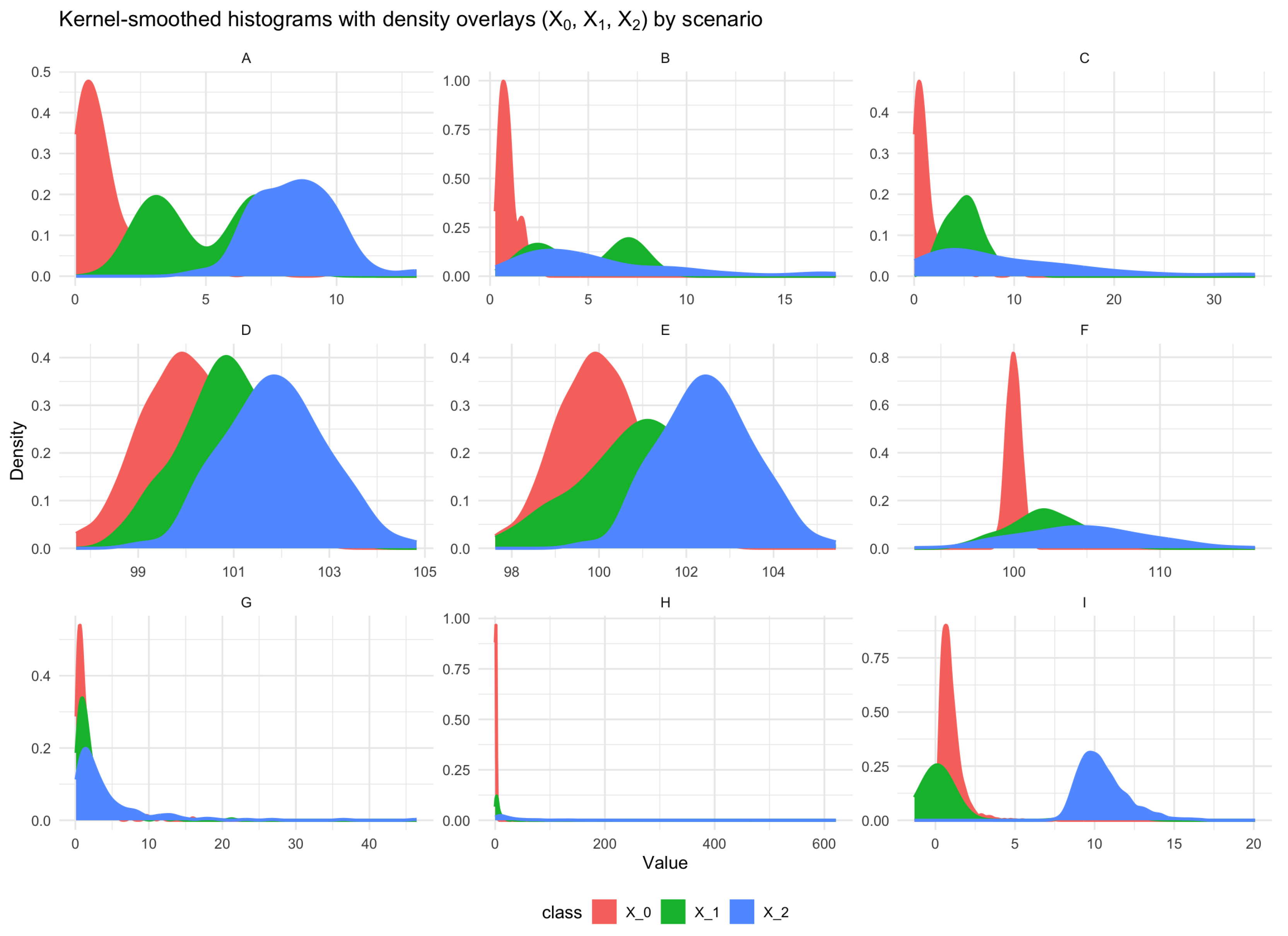
Figure 2.
Visual representation of results for the simulation scenarios considered.
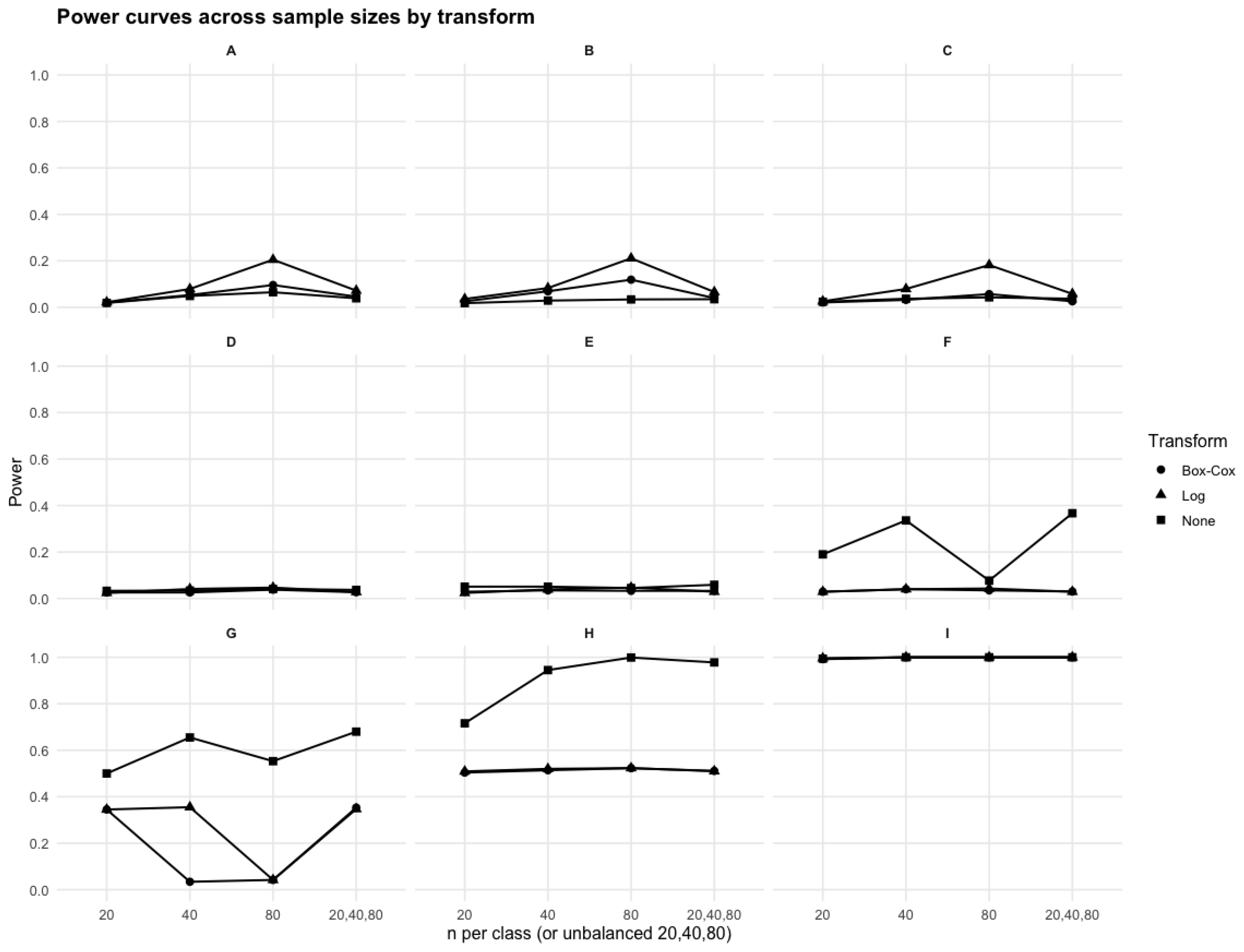
Figure 3.
Raw and kernel smoothed histograms (left) along with corresponding boxplots (right) for the crude data (top row) and log transformed data (bottom row) of Covid-19 antibody data after the first dose of the BNT162b2 vaccine by age group.
Figure 3.
Raw and kernel smoothed histograms (left) along with corresponding boxplots (right) for the crude data (top row) and log transformed data (bottom row) of Covid-19 antibody data after the first dose of the BNT162b2 vaccine by age group.
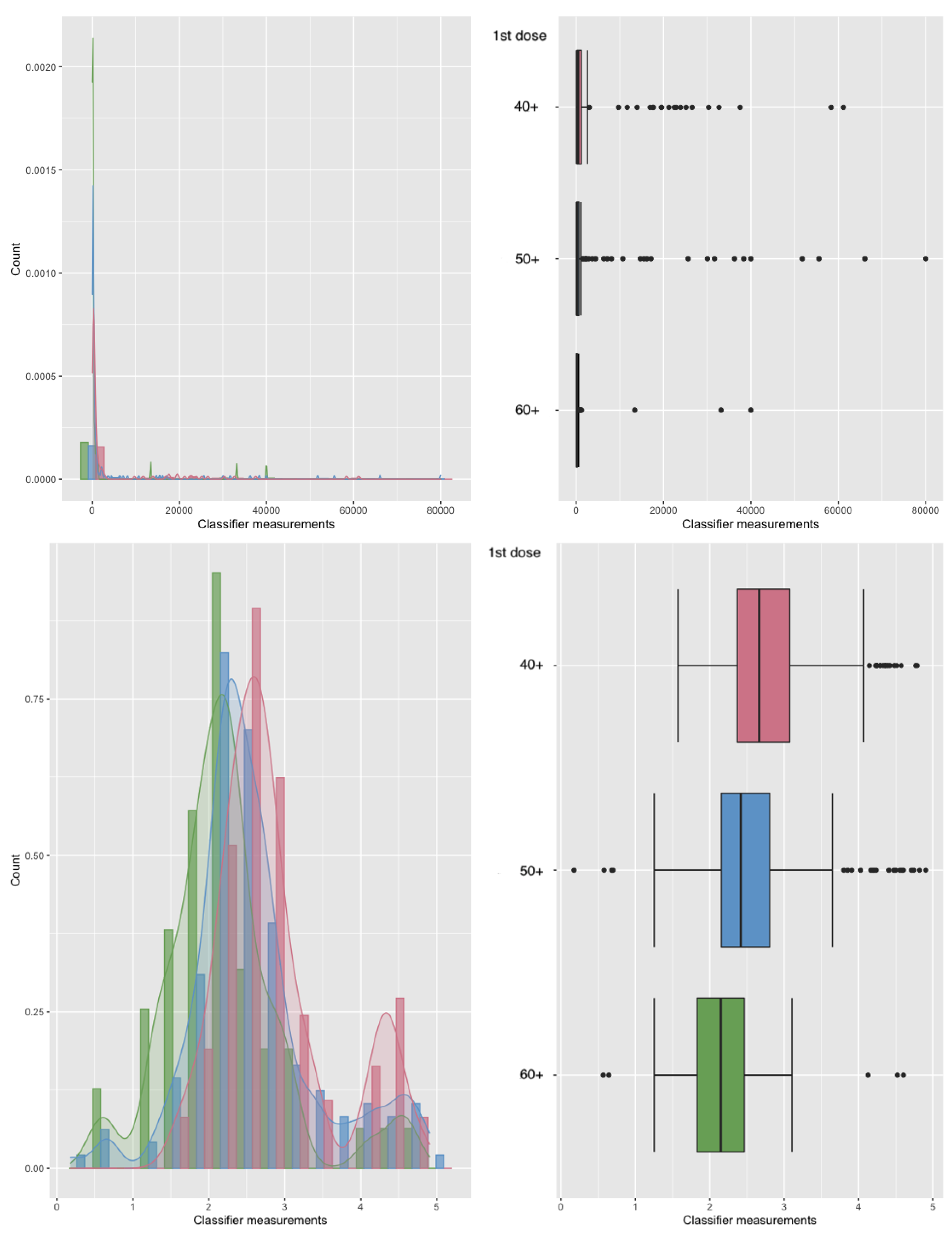
Figure 4.
ROC surfaces by estimation approach for the Covid-19 antibody data after the first dose of the BNT162b2 vaccine, illustrating the separation between three major age groups (1: 60-69, 2: 50-59, 3: 40-49). Panels shown, A: Empirical, B: Naive trinormal, C: Trinormal after log transformation, D: Trinormal after Box–Cox.
Figure 4.
ROC surfaces by estimation approach for the Covid-19 antibody data after the first dose of the BNT162b2 vaccine, illustrating the separation between three major age groups (1: 60-69, 2: 50-59, 3: 40-49). Panels shown, A: Empirical, B: Naive trinormal, C: Trinormal after log transformation, D: Trinormal after Box–Cox.
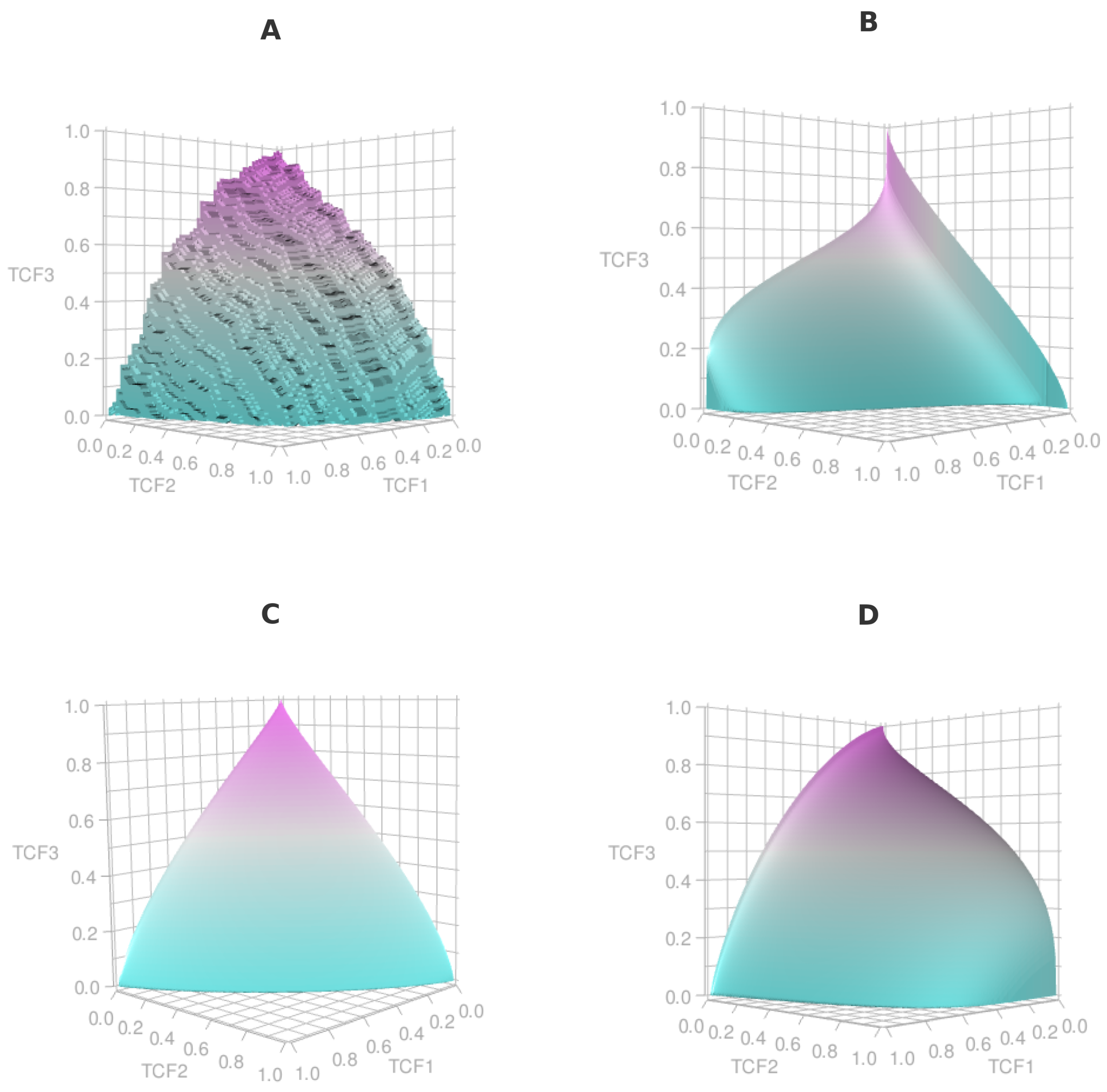

Table 1.
Empirical VUS vs naive trinormal plug-in VUS (Scenarios A–I). Sample sizes of 2000, averages of r=300000 replicates given for empirical and naive trinormal VUS.
Table 1.
Empirical VUS vs naive trinormal plug-in VUS (Scenarios A–I). Sample sizes of 2000, averages of r=300000 replicates given for empirical and naive trinormal VUS.
| Scenario (approximate target empirical VUS) | Empirical VUS | Naive trinormal VUS | |||
|---|---|---|---|---|---|
| A () | 0.818 | 0.811 | |||
| B () | 0.555 | 0.562 | |||
| C () | 0.592 | 0.584 | |||
| D () | 0.504 | 0.511 | |||
| E () | 0.523 | 0.525 | |||
| F () | 0.493 | 0.507 | |||
| G () | 0.295 | 0.209 | |||
| H () | 0.699 | 0.427 | |||
| I () | 0.214 | 0.602 |
1 Notes: is Normal with mean and variance , with for scenarios D-F. is Gamma with shape k and scale . , denoted as , uses as log-scale parameters (meanlog, sdlog). Mixture weights are shown explicitly; e.g., .
Table 2.
Monte Carlo power by scenario. Entries are rejection proportions over replicates for balanced designs (n per class) and the unbalanced design .
Table 2.
Monte Carlo power by scenario. Entries are rejection proportions over replicates for balanced designs (n per class) and the unbalanced design .
| Unbalanced | ||||||||||||
|---|---|---|---|---|---|---|---|---|---|---|---|---|
| Scenario | Box–Cox | Log | None | Box–Cox | Log | None | Box–Cox | Log | None | Box–Cox | Log | None |
| A | 0.020 | 0.022 | 0.019 | 0.053 | 0.079 | 0.049 | 0.096 | 0.205 | 0.065 | 0.046 | 0.072 | 0.039 |
| B | 0.026 | 0.036 | 0.018 | 0.069 | 0.083 | 0.029 | 0.119 | 0.211 | 0.034 | 0.040 | 0.066 | 0.035 |
| C | 0.021 | 0.026 | 0.024 | 0.032 | 0.079 | 0.037 | 0.057 | 0.182 | 0.043 | 0.026 | 0.058 | 0.037 |
| D | 0.026 | 0.024 | 0.033 | 0.026 | 0.041 | 0.034 | 0.038 | 0.047 | 0.041 | 0.027 | 0.028 | 0.037 |
| E | 0.029 | 0.024 | 0.051 | 0.035 | 0.039 | 0.051 | 0.033 | 0.047 | 0.045 | 0.033 | 0.029 | 0.059 |
| F | 0.029 | 0.029 | 0.190 | 0.040 | 0.040 | 0.336 | 0.035 | 0.043 | 0.077 | 0.030 | 0.029 | 0.367 |
| G | 0.345 | 0.345 | 0.500 | 0.034 | 0.355 | 0.655 | 0.042 | 0.042 | 0.553 | 0.353 | 0.347 | 0.680 |
| H | 0.504 | 0.509 | 0.716 | 0.514 | 0.520 | 0.945 | 0.523 | 0.523 | 0.999 | 0.511 | 0.510 | 0.978 |
| I | 0.992 | 0.996 | 0.994 | 1.000 | 1.000 | 1.000 | 1.000 | 1.000 | 1.000 | 1.000 | 1.000 | 1.000 |
Table 3.
Results of trinormal goodness-of-fit tests under different transformations.
| Case | VUS empirical | VUS trinormal | D | p-value |
|---|---|---|---|---|
| None | 0.335 | 0.180 | 3.865 | 1.11e-04 |
| Log | 0.335 | 0.295 | 2.254 | 0.024 |
| Box–Cox | 0.335 | 0.306 | 1.674 | 0.094 |
Disclaimer/Publisher’s Note: The statements, opinions and data contained in all publications are solely those of the individual author(s) and contributor(s) and not of MDPI and/or the editor(s). MDPI and/or the editor(s) disclaim responsibility for any injury to people or property resulting from any ideas, methods, instructions or products referred to in the content. |
© 2025 by the authors. Licensee MDPI, Basel, Switzerland. This article is an open access article distributed under the terms and conditions of the Creative Commons Attribution (CC BY) license (http://creativecommons.org/licenses/by/4.0/).
Copyright: This open access article is published under a Creative Commons CC BY 4.0 license, which permit the free download, distribution, and reuse, provided that the author and preprint are cited in any reuse.