Submitted:
09 September 2025
Posted:
09 September 2025
You are already at the latest version
Abstract
In Global Navigation Satellite System (GNSS)-denied environments, Unmanned Aerial Vehicles (UAVs) relying on Vision-Based Navigation (VBN) in high-altitude, moun-tainous terrain face severe challenges due to geometric distortions in aerial imagery. This paper proposes a georeferenced localization framework that integrates orthorec-tified aerial imagery with Scene Matching (SM) to achieve robust positioning. The method employs a camera projection model combined with Digital Elevation Model (DEM) to orthorectify UAV images, thereby mitigating distortions from central projec-tion and terrain relief. Pre-processing steps—including illumination normalization, lens distortion correction, rotational alignment, and resolution adjustment—enhance consistency with reference orthophoto maps, after which template matching is per-formed using Normalized Cross-Correlation (NCC). Sensor fusion is achieved through Extended Kalman Filter (EKF) incorporating Inertial Navigation System (INS), GNSS (when available), barometric altimeter, and SM outputs, with sub-modules for hori-zontal, vertical, and altimeter error estimation. The framework was validated through flight tests with an aircraft over 45 km trajectories at altitudes of 2.5 km and 3.5 km in mountainous terrain. Results demonstrate the orthorectification improves image simi-larity and significantly reduces localization error, yielding lower 2D RMSE compared to conventional rectification. The proposed approach enhances VBN by mitigating terrain-induced distortions, providing a practical solution for UAV localization in GNSS-denied scenarios.
Keywords:
UAV localization
; vision-based navigation
; scene matching
; orthorectification
; GNSS-denied
; mountainous terrain
1. Introduction
Unmanned Aerial Vehicles (UAVs) are pivotal in applications such as exploration, disaster response, and surveillance [1]. Traditionally, an integrated navigation system that combines Inertial Navigation System (INS) and Global Navigation Satellite System (GNSS) has provided reliable positioning for UAVs. However, GNSS is vulnerable to signal blockage and interference, leading to GNSS-denied environments, such as urban canyons, indoor settings, or areas with adversarial jamming [2,3]. In such scenarios, INS errors accumulate rapidly, leading to significant positional drift and necessitating robust alternative navigation techniques to ensure stable and accurate localization.
Vision-Based Navigation (VBN) has emerged as a promising approach for GNSS-denied environments, driven by advances in camera miniaturization, image sensor technology, computing technology, and image processing algorithms [4]. VBN techniques can be categorized into three primary approaches based on their use of maps: Visual Odometry (VO), which incrementally estimates motion without relying on maps; Visual Simultaneous Localization and Mapping (VSLAM), which concurrently builds and uses environmental maps for localization; and Scene Matching (SM), which determines position by comparing current images with pre-built maps [5].
VO estimates UAV position and orientation in real time by analyzing visual data from consecutive image frames. To improve robustness, VO is often integrated with Inertial Measurement Unit (IMU) data, a technique referred to as Visual Inertial Odometry (VIO). Due to its cost-effectiveness, VO has been widely adopted in commercial UAVs [6,7]. However, VO relies on relative motion estimation through techniques such as optical flow, leading to inevitable error accumulation over time [8]. VSLAM mitigates this by simultaneously estimating position and constructing maps, using techniques like loop closure and bundle adjustment to correct errors [9,10]. Nevertheless, VSLAM faces challenges in expansive outdoor environments where loop closure opportunities are limited, resulting in gradual error accumulation.
In contrast, SM provides absolute positioning by comparing aerial images with pre-built map data—such as satellite imagery, orthophoto maps, or 3D models— thereby avoiding cumulative errors inherent in VO and VSLAM [11]. By leveraging absolute coordinates, SM maintains consistent global positioning when high-quality map data is available. Its robustness in texture-rich environments and compatibility with wide fields of view at high altitudes make it particularly effective for GNSS-denied navigation in outdoor UAV operations.
The most challenging aspect of SM-based localization is the need to match heterogeneous images captured under varying conditions, such as different viewpoints, illumination, sensors, and resolutions. Previous studies have explored several approaches to address these difficulties. Traditional template matching methods have employed diverse similarity metrics between reference images and aerial imagery. Conte et al. [12] proposed a VBN architecture that integrates inertial sensors, VO, and image registration to a georeferenced image. Their system, using Normalized Cross-Correlation (NCC) as the matching metric, reported a maximum positional error of 8 m in a 1 km closed-loop trajectory at 60 m altitude. Yol et al. [13] applied Mutual Information (MI)-based matching, achieving RMSE values of 6.56 m (latitude), 8.02 m (longitude), and 7.44 m (altitude) in a 695 m flight test at 150 m altitude. Sim et al. [14] proposed an integrated system that estimates aircraft position and velocity using sequential aerial images. They employed Robust Oriented Hausdorff Measure (ROHM) for the image matching, and flight tests with helicopters and aircraft at altitudes up to 1.8 km and distances up to 124 km showed errors on the order of hundreds of meters. Wan et al. [15] introduced an illumination-invariant Phase Correlation (PC) method to match aerial images with reference satellite imagery. In their study, aerial images captured by a UAV flying at an average altitude of 350 m were roughly rectified to a nadir view, and the average positioning errors were reported as 32.2 m along the x-axis and 32.46 m along the y-axis.
Numerous deep learning-based methods have also been reported. To handle differences in viewpoint and seasonal appearance, Goforth et al. [16] combined CNN features trained on satellite data with temporal optimization that minimizes alignment errors across frames, achieving an average localization error of less than 8 meters for an 850 m flight at 200 m altitude. Gao et al. [17] employed a deep learning image registration network, combining SuperPoint [18] and SuperGlue [19], for high-precision feature point extraction and matching, achieving sub-pixel accuracy (within 2 pixels). Sun et al. [20] utilized Local Feature Transformer (LoFTR) to enable robust matching in low-texture indoor environments, overcoming limitations of local feature-based methods. Hikosaka et al. [21] proposed extracting road networks from aerial and satellite images using a U-Net-based deep learning model, followed by template matching. Although the method achieved sub-pixel registration accuracy even for images with distant acquisition times, its applicability is restricted in mountainous areas with sparse road networks and relies on nadir-view aerial images from the Geospatial Information Authority, limiting its use for oblique-view UAV imagery.
As shown in Figure 1, distortions occur in aerial images depending on the camera's viewpoint and terrain elevation. To improve localization accuracy affected by viewpoint differences when observing terrain, several studies have been conducted. Woo et al. [22] proposed a method for estimating UAV position and orientation by matching oblique views of mountain peaks with Digital Elevation Models (DEMs), but validation was limited to simulations, restricting its generalizability. Kinnari et al. [23] performed orthorectification of UAV images to match them with reference images; however, this approach assumes local planarity of the environment, converting images to a nadir view, which limits its effectiveness in rugged terrains with significant elevation changes, such as mountainous areas. Chiu et al. [24] used a 3D georeferenced model to render reference images in an oblique view similar to the UAV images for matching, reporting RMSE errors of 9.83 m over 38.9 km; however, information about the map and flight altitude was not specified. Ye et al. [25] employed a coarse-to-fine approach for oblique-view images, but their tests were conducted with images captured by a UAV flying at 150 m altitude over a university campus with many buildings, limiting applicability to natural terrains.
Despite these advances, most studies have focused on low-altitude flights in flat or texture-rich environments, with limited analysis of geometric distortions caused by significant terrain variations at high altitudes (above 2 km) [26]. This study addresses these gaps by analyzing the impact of terrain-induced geometric distortions on localization accuracy in high-altitude UAV imagery and proposes a VBN architecture using a novel SM method that integrates orthorectification to enhance consistency with reference maps. The proposed approach is validated through experiments in rugged mountainous environments, demonstrating its effectiveness for stable and accurate absolute navigation in GNSS-denied settings.
The main contributions of this work are as follows:
- A VBN architecture and SM technique efficient for high-altitude UAV localization in mountainous terrain.
- Orthorectification of aerial imagery using a projection model and DEM to mitigate geometric distortions, thereby improving matching accuracy with orthophoto maps.
- Validation in real flight experiments over mountainous regions.
2. Methods
This section provides an overview of the proposed VBN algorithm for high-altitude UAV position estimation in mountainous terrain, followed by detailed descriptions of its components. The algorithm integrates data from an IMU, a GNSS receiver, a barometric altimeter, and a camera to achieve robust geolocation, particularly in GNSS-denied environments. Orthorectification and an Extended Kalman Filter (EKF) are employed to mitigate terrain-induced distortions and fuse sensor measurements, respectively.
2.1 Overview
The proposed method combines INS, GNSS, barometric altimetry, and SM to estimate the UAV’s position, velocity, and attitude. Figure 2 presents a block diagram of the algorithm, illustrating the data flow and processing stages. The key components are as follows:
- Input Data: Measurements from the IMU, GNSS, barometric altimeter, and camera, along with reference data including orthophoto maps and DEMs. When GNSS is available, the GNSS navigation solution is used to correct INS errors; otherwise, the SM result is used.
- INS Mechanization: The IMU outputs are processed to compute the UAV’s position, velocity, and attitude using INS mechanization.
- Aerial Scene Matching: Aerial images are compared with the georeferenced orthophoto map to estimate the UAV’s position. Orthorectification is applied to compensate for terrain-induced geometric distortions using DEM data. Aerial images undergo image processing to achieve consistent resolution, rotation, and illumination with georeferenced images.
- Sensor Fusion: The proposed method employs three EKF-based sub-modules for sensor fusion: a 13-state EKF for horizontal navigation errors, attitude errors, and sensor biases; a 2-state EKF for vertical channel (altitude) stabilization; and a 2-state error estimator for the barometric altimeter. These sub-modules collectively produce a corrected navigation solution.
2.2 Aerial Scene Matching
SM is a fundamental technique for estimating the absolute position of UAVs by registering aerial imagery with georeferenced images. This process enables the computation of the UAV's position. This subsection details the key components of SM, including the role of georeferenced images, the orthorectification for UAV imagery, and image processing techniques using template matching. The flow chart of SM is shown in Figure 3.
2.2.1. Georeferenced image
Georeferenced images are essential for SM, serving as the reference dataset to which UAV-captured imagery is registered. These images are embedded with geographic coordinates in a standard Coordinate Reference System (CRS), such as WGS84 (EPSG:4326) or Universal Transverse Mercator (UTM), enabling pixel-to-geospatial coordinate mapping. To maximize the SM accuracy for UAV localization, georeferenced images should be ideally in the form of orthophotos, which are orthorectified to eliminate geometric distortions caused by terrain relief, camera tilt, and lens imperfections. This ensures that each pixel in the georeferenced image corresponds precisely to the geographic location of the actual terrain.
2.2.2. Orthorectification
Accurate and precise UAV localization requires transforming UAV-captured images into a form consistent with georeferenced orthophoto maps. Geometric distortions induced by terrain relief are a primary factor degrading the accuracy of SM for UAV position estimation. These distortions arise from the central projection of the camera and the three-dimensional characteristics of the terrain. To mitigate these effects, this subsection proposes an orthorectification technique applied to UAV imagery, transforming it into a form consistent with reference orthophoto maps, thereby enhancing SM performance and minimizing geolocation errors.
The orthorectification process for UAV images is summarized as follows:
- Projection Model Development: A projection model is created using the camera’s intrinsic (e.g., focal length) and extrinsic (e.g., position and attitude) parameters [27]. The camera position and attitude information determining the projection model uses aided navigation information estimated through the sensor fusion framework (Section 2.3).
- Pixel-to-Terrain Projection: The projection path for each pixel in the image sensor is computed based on the projection model.
- Pixel Georeferencing: Using the DEM, the intersection between each pixel's projection line and the terrain is determined, yielding the actual geographic coordinates corresponding to each image pixel.
- Reprojection and Compensation: The image is reprojected to compensate for terrain relief displacements, aligning each pixel with its actual geographic location.
- Orthorectification using Camera Projection Model
- The following describes the detailed procedure for calculating the actual geographic coordinates of terrain points corresponding to each pixel in a UAV-captured image. The method is formulated using the camera projection model and DEM. For clarity, Figure 4 illustrates a cross-sectional view () under the assumption of a pitch angle . Boldface symbols are used to represent vectors.
The world coordinate system (W-frame), UAV body coordinate system (B-frame), and camera coordinate system (C-frame) are depicted in Figure 4, where the superscripts of the origin and the x, y, z axes indicate the corresponding frame. For example, and , , denote the origin and the axes of the W-frame, respectively. The rotation matrix () from the B-frame to the W-frame, defined by Euler angles, is given as:
where , , represent roll, pitch, and yaw, respectively.
The rotation matrix () from the B-frame to the C-frame is:
Thus, the rotation matrix () from the C-frame to the W-frame is obtained as:
The origins of the C-frame and B-frame are assumed to coincide with the focal point of the camera. and are located at in the W-frame, where denotes the UAV altitude. The image plane of the camera is positioned at a distance equal to the focal length () from , with the camera oriented according to the UAV’s attitude.
Orthorectification reprojects each pixel (index ) in the original UAV image to a corresponding pixel in the orthorectified image, thereby compensating for terrain-induced displacements. The terrain elevation is obtained from the DEM.
The coordinates of the -th pixel in the C-frame are given by:
where and are the image plane coordinates, and denote the image width and height in pixels, and μ is the pixel pitch.
The coordinates in the W-frame are obtained by applying the rotation matrix () and a translation by altitude:
The projection line for pixel passes through and in the W-frame. The line equation can be expressed in vector (parametric) form as:
where , , and are the x-, y- and z-components of , and is a real-valued parameter.
The intersection between the projection line and the terrain elevation is computed iteratively, as described in Algorithm 1 and illustrated in Figure 4. The horizontal coordinate of , denoted , represents the actual geographic position corresponding to the -th pixel in the orthorectified image. Once the terrain intersections for all UAV image pixels are determined using Algorithm 1, the pixels are reprojected onto a regular grid, thereby generating the orthorectified image.

| Algorithm 1 Fixed-Point Iteration for Finding Intersections of a 3D Line and a Discretized Data Surface |
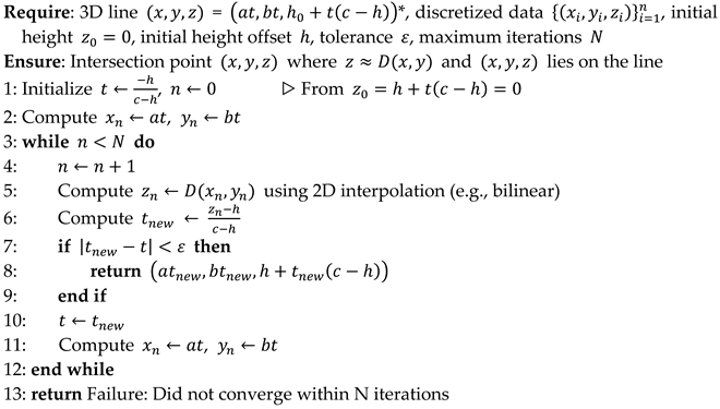 |
* The line is defined by the camera image pixel position (a, b, c) and the reference point (0, 0, h) in the W-frame.
Orthorectification Results
The results of the proposed orthorectification method are presented in Figure 5. Figure 5a shows the original aerial image acquired at an altitude of 3.5 km, with the camera oriented at a roll angle of 5° and a pitch angle of 3°. The DEM of the imaged terrain is given in Figure 5b, where the elevation varies within a range of 100–420 m. Figures 5c and 5d are the rectified image and the orthorectified image, respectively. The rectified image is obtained by applying a homography transformation to align the image plane parallel to the ground surface, effectively converting the oblique view into a nadir view. Figure 5d shows the orthorectified image generated using the method proposed in this study.
A pixel-wise comparison between the rectified and orthorectified images is provided in Figures 5e and 5f. Figure 5e presents a red–cyan composite of the two images, while Figure 5f illustrates the difference mask, where pixels with an intensity discrepancy exceeding a tolerance of 50 are highlighted in white. The correspondence between the white regions in Figure 5f and areas of higher or lower terrain elevation in the DEM confirms that terrain-induced displacements are strongly correlated with terrain elevation.
Image matching was conducted by registering both the rectified and orthorectified images with the reference orthophoto map (Figure 5g and 5h). For the rectified image (Figure 5c), template matching using NCC yielded a maximum similarity score of 0.303. In contrast, the orthorectified image (Figure 5d) achieved a score of 0.480, corresponding to an absolute increase of 0.177 in similarity with the reference map. Furthermore, the localization error obtained from template matching was reduced from 15.8 m to 9.5 m. A detailed comparison of the geolocation errors estimated through template matching is provided in Section 3.2. These results demonstrate that the proposed orthorectification method effectively mitigates terrain-induced distortions, thereby improving the accuracy of SM and geolocation in mountainous environments.
2.2.3. Image Processing and Matching
The primary difficulty in SM lies in registering two heterogeneous images with differing characteristics, such as variations in illumination, resolution, and perspective. At high altitudes (e.g., several kilometers), the distinctiveness of keypoints, such as building corners or road intersections, diminishes due to their smaller apparent size, making traditional feature-based methods like Scale-Invariant Feature Transform (SIFT) or Speeded-Up Robust Features (SURF) less effective. In mountainous regions, where distinct geometric structures like roads or buildings are scarce, feature-based matching is particularly challenging. Consequently, template matching, which relies on global pattern comparison, is employed as a more suitable approach for SM in such environments.
To achieve consistent image registration between UAV imagery and georeferenced images, the following pipeline is implemented, as illustrated in Figure 3:
- Illumination Normalization: Histogram equalization or Contrast-Limited Adaptive Histogram Equalization (CLAHE) [28] is applied to both UAV images and georeferenced images to mitigate variations in lighting and contrast, ensuring robustness across diverse environmental conditions.
- Lens Distortion Correction: UAV images are corrected for lens-induced distortions using pre-calibrated intrinsic camera parameters and distortion coefficients, ensuring accurate spatial geometry.
- Resolution Adjustment: To ensure spatial consistency between the UAV image and the georeferenced map, the UAV image is rescaled based on the aided altitude. The scaling factors in the and directions are computed as:
- where is the flight altitude above ground, is the reference map resolution, and is the focal length.
- Orthorectification: Orthorectification is performed to remove geometric distortions in aerial imagery caused by camera position, attitude, and terrain elevation variations, thereby ensuring consistency with the georeferenced orthophoto maps (Section 2.2.2).
- Rotational Alignment: Before template matching, the georeferenced image and the aerial image should be rotationally aligned using the UAV’s attitude data. The orthorectified aerial image shows a ground footprint rotated by the UAV’s heading. Since template matching is carried out by sliding a rectangular template over the georeferenced image, the orthorectified image would be excessively cropped without alignment. To minimize this effect, both the orthorectified image and the georeferenced image are rotated by the UAV’s heading angle, thus achieving rotational alignment. This rotation is implemented using a 2D affine transformation matrix defined as
- where denotes the UAV heading angle and is the rotation center.
- Template Matching: Following the preprocessing, template matching is employed to estimate the UAV’s position by correlating the UAV image (template) with a reference image. The similarity between the template and a region of the reference image is measured using NCC [29], which is known for robustness against linear illumination variations. NCC computes the normalized correlation coefficient between the template and a sliding window in the reference image.
- The NCC at position in the reference image is defined as:
- where and are indices spanning the template dimensions, is pixel intensity in the reference image at position , relative to the top-left corner of the window at , is pixel intensity in the template at position , is mean intensity of the reference image window with top-left corner at , and is mean intensity of the template.
-
The estimated UAV position is obtained as:The step-by-step application of the signal processing described above is illustrated in Figure 6.
2.3 Sensor Fusion
The EKF [30] integrates inertial navigation outputs with external measurements to refine localization accuracy (Figure 7). The framework consists of three components: a horizontal channel filter, a vertical channel filter, and a barometric altimeter error estimator.
2.3.1. Horizontal Channel EKF
The horizontal-channel EKF fuses INS navigation states with external measurements from GNSS or SM. The state vector is defined as:
where , denote latitude and longitude errors, , are velocity errors in the east and north directions, , , are attitude (pitch, roll, yaw), and and represent accelerometer and gyro biases along -axis, respectively.
The measurement vector consists of the differences between the INS position and those obtained from GNSS or SM. For synchronization, the navigation states are stored in the INS buffer at 300 Hz. Time synchronization between the INS and GNSS is achieved using the Pulse Per Second (PPS) signal, whereas synchronization with SM is performed based on the image acquisition time. In this process, the latency between aerial image capture and its delivery to the filter is pre-measured and compensated. For instance, in the flight tests described in Section 3, the latency of the aerial image was measured to be approximately 170 ms.
Measurement updates in the EKF are performed based on a priority scheme, where GNSS measurements have higher priority than SM measurements. That is, when GNSS measurements are available, they are used to update the EKF, whereas in GNSS-denied environments, SM measurements are employed for the update. The measurement models are:
where and denote latitude and longitude, respectively.
2.3.2. Vertical Channel EKF
Errors in the vertical channel of the INS diverge rapidly compared to the horizontal channel, necessitating external altitude stabilization. In this study, altitude stabilization is achieved by using GNSS altitude whenever available and barometric altitude otherwise. When GNSS altitude is available, it is also used to estimate the bias and scale-factor error of the barometer. This ensures consistency of barometric altitude with the WGS-84 reference, even during GNSS outages.
The state vector for the vertical channel is:
where and denote altitude and vertical velocity errors, respectively.
2.3.3. Barometric Altimeter Error Estimator
The barometric altimeter error estimator [31] operates jointly with the vertical channel filter. When GNSS altitude is available, it estimates the barometer bias and scale factor error, enabling correction of barometer altitude during GNSS outages. The state vector is:
and the measurement model is defined as:
The corrected barometric altitude is then computed as:
which ensures alignment with GNSS altitude in the WGS-84 datum.
3. Experimental Setups and Results
This section describes the experimental setup and the geolocation performance evaluation of the proposed VBN algorithm, specifically designed for UAV position estimation in mountainous terrain.
3.1. Experiment on Real Flight Aerial Image Dataset
Flight tests were conducted using a Cessna 208B aircraft, equipped with onboard sensors including an IMU, a GNSS receiver, a downward-facing camera, a barometer altimeter, and a signal processing computer (Figure 8). This configuration enabled the collection of a comprehensive dataset for evaluating the performance of both VBN and SM.
3.1.1. Sensor Specification
The specifications of the onboard sensors are summarized in Table 1. The camera was equipped with a 16 mm focal length lens, providing a horizontal field of view (HFOV) of 37.84° and a vertical field of view (VFOV) of 29.19°. The original images were captured at a resolution of 4096×3000 pixels, but they were downsampled by a factor of ¼ to create an image dataset of 1024×750 pixels. The camera’s frame rate is 1 Hz. At an altitude of 3 km, this corresponds to a Ground Sample Distance (GSD) of approximately 2 m. The IMU included accelerometers with a 300 Hz output rate and a bias of 60 µg, and gyroscopes with a 300 Hz output rate and a bias of 0.04°/h. The barometer provided altitude measurements at a 5 Hz output rate, serving as an external source to constrain divergence in the vertical channel of the INS.
3.1.2. Flight Scenarios and Dataset Characteristics
The dataset was collected over five flight paths across two distinct mountainous regions with significant terrain elevation variations, as illustrated in Figure 9 and summarized in Table 2. Paths 1 to 3, with headings -172.9° (north-to-south), -8.4° (south-to-north), and -176.9° (north-to-south), covered one region at altitudes of 3.5 km (Paths 1 and 2) and 2.5 km (Path 3). Paths 4 and 5, with headings 6.6° (south-to-north) and -165.4° (north-to-south), covered another region at 2.5 km altitude. Each path spanned approximately 45 km over 9 minutes at 300 km/h. Aerial images captured by the camera yielded a GSD of approximately 2.3 m at 3.5 km altitude and 1.5 m at 2.5 km altitude. This design enabled evaluation of the algorithm’s robustness under diverse flight directions, altitudes, and terrain conditions.
3.1.3. Data Processing
The collected dataset was processed in post-flight simulations to evaluate the proposed algorithm. Aerial images were orthorectified using aided navigation information to correct terrain-induced geometric distortions, ensuring geometric consistency with the reference orthophoto maps. Differential Global Positioning System (DGPS) data provided high-precision ground truth for validating horizontal position.
3.2. Localization Accuracy
Figure 10 illustrates the localization errors obtained from SM between the captured aerial imagery and georeferenced orthophoto maps. Figure 10a shows the results obtained using conventional rectification, whereas Figure 10b presents the results using the proposed orthorectification method.
In Figure 10a, a substantial increase in localization error is observed in areas with significant terrain elevation changes (as shown in Figure 9c). Furthermore, improving the map resolution from 8 m to 2 m provides only marginal benefits in position accuracy when conventional rectification is applied. In contrast, Figure 10b demonstrates a considerable reduction in localization error compared to Figure 10a. Notably, as the reference map resolution improves from 8 m to 2 m, localization accuracy shows a marked enhancement, underscoring the effectiveness of the proposed orthorectification approach in mitigating terrain-induced errors.
The performance of the proposed VBN algorithm—integrating SM with orthorectification and the sensor fusion framework—was evaluated under GNSS-denied environments, with results summarized in Table 3 and Figure 11. The results are organized according to flight paths, map resolution, and the use of orthorectification. Localization accuracy was assessed using the two-dimensional root-mean-square error (2D RMSE). Table 3 confirms that the applying orthorectification consistently improves localization accuracy across various flight paths and map resolutions. The improvement is particularly pronounced for Flight Path 5. Flight Paths 4 and 5 involve steeper terrain and lower altitudes (approximately 1 km lower than other paths), presenting more challenging conditions for SM. These conditions lead to a higher incidence of false matching and increased distortion in the aerial imagery.
Nevertheless, the proposed orthorectification method effectively mitigates localization errors even in such challenging scenarios. Increasing the resolution of the reference map further enhanced positioning accuracy when orthorectification was applied, whereas the rectification approach provided limited improvements. Furthermore, as shown in Figure 11, localization error decreases as map resolution improves, in contrast to the limited improvements observed when conventional rectification is applied. The proposed method achieves improved localization accuracy, with errors consistently on average 1.4 pixels of the map resolution across all tested conditions. These results highlight the robustness and effectiveness of the proposed VBN algorithm in supporting UAV navigation in GNSS-denied environments.
Figure 12 presents the navigation errors for Flight Path 2 in a GNSS-denied environment, utilizing a 4 m resolution orthophoto map. The proposed VBN algorithm is compared with INS and VBN with rectified aerial images. INS exhibits a gradual increase in localization error over time, and INS accumulates a position error of approximately 300 m over an 8.5-minute flight duration. The VBN with conventional rectification yields a final position error of 10.2 m, with errors remaining within 30 m. By contrast, the proposed method achieves a final position error of only 2.9 m, maintaining errors within 10 m throughout the entire flight. These results demonstrate that the proposed VBN algorithm is a viable alternative to GNSS in GNSS-denied environments. Moreover, the algorithm significantly reduces localization errors for UAVs operating at high altitudes over mountainous terrain, thereby ensuring reliable navigation performance under challenging conditions.
4. Discussion
The proposed orthorectification method relies on the UAV’s position and attitude information. In this process, the UAV’s attitude determines the geometry of camera projection rays, while horizontal position errors induce inaccuracies in the elevation retrieved from the DEM. Additionally, altitude errors affect the projection distance, influencing the scaling of the captured imagery.
The experiments in Section 3 assumed a scenario where the UAV initially operates in a GNSS-available environment before transitioning to a GNSS-denied condition, with SM outputs used to update the EKF. This implies that INS position, velocity, and attitude errors are well-corrected in GNSS-available conditions, resulting in minimal navigation errors at the beginning of GNSS-denied operation.
This section provides an additional analysis of how aided navigation errors affect the performance of the proposed SM. Simulations were conducted for three cases summarized in Table 4. As described in Section 3.1.1, the IMU used in this study has a gyro bias of 0.04°/h and an accelerometer bias of 60 µg. With such specifications, the expected alignment performance corresponds to approximately 0.003° in horizontal attitude error and 0.2° in yaw error [30]. To reflect more challenging conditions, the attitude errors were set to values more than ten times larger: roll/pitch errors of 0.03/0.05/0.1°, and yaw errors of 0.5/1.0/1.5°. The position errors were defined as 10/20/30 m in latitude and longitude, and 20/40/60 m in altitude, reflecting typical GNSS receiver accuracies. Simulations were carried out using the Flight Path 2 dataset with 4 m resolution georeferenced maps, and the results are presented in Figure 13 and Table 5.
Figure 13a illustrates the SM results with orthorectification applied, while Figure 13b corresponds to conventional rectification. In Figure 13a, the SM position error gradually increases as the navigation errors grow. In Case 3, where the largest errors are introduced, terrain-induced distortions are not fully compensated, resulting in errors comparable to those observed with rectification (Figure 13b). Table 5 summarizes the performance of the VBN algorithm when using the SM outputs as measurements. Although these errors lead to a slight degradation in performance, the impact remains within tolerable range.
These findings demonstrate that the proposed SM and VBN method maintains reliable localization accuracy even in the presence of moderate navigation errors, highlighting its robustness for practical UAV operations in GNSS-denied environments.
5. Conclusions
This study proposed a VBN framework that integrates orthorectification-based SM with INS- and barometer-aided sensor fusion for UAV operations in GNSS-denied environments. By compensating for terrain-induced distortions, the method consistently improved localization accuracy across different flight paths and reference map resolutions.
The experimental results using real aerial flight data demonstrated that the proposed framework achieves an average localization accuracy of 1.4 pixels. The findings confirm that orthorectification is a critical step for enhancing the reliability of SM, especially in mountainous terrain where geometric distortions are significant. In particular, the framework maintained stable performance in challenging cases such as steep relief and high-altitude imagery, where conventional rectification methods typically produce large errors. These contributions establish the proposed framework as a viable alternative to GNSS in environments where satellite signals are unavailable, degraded, or intentionally denied.
Despite these promising results, several limitations remain. The flight trajectories used in this study were limited to straight paths at altitudes of 2.5–3.5 km. At lower altitudes over mountainous terrain, the reduced image footprint is expected to make matching more difficult. Moreover, although the dataset was systematically constructed through real flight tests with synchronized INS, camera, GNSS, and barometer measurements, the validation was performed in an offline environment rather than in real time. Finally, the IMU employed was of navigation grade, which may not fully represent the performance achievable with lower-cost sensors.
Future work will address these limitations in several directions: (i) optimizing the algorithm for real-time onboard implementation on resource-constrained UAV hardware; (ii) extending validation to diverse flight trajectories and altitudes, including low-altitude UAV flights in mountainous terrain; and (iii) investigating the applicability of the framework with low-cost MEMS-grade IMUs to broaden its practicality for small UAVs.
Author Contributions
Conceptualization, I.L. and C.-K.S.; methodology, I.L.; software, I.L. and H.L.; validation, I.L. and S.N.; formal analysis, I.L.; investigation, I.L. and C.P.; resources, J.O. and K.L.; data curation, J.O.; writing—original draft preparation, I.L.; writing—review and editing, I.L.; visualization, I.L.; supervision, I.L. and C.P.; project administration, J.O. and C.-K.S. All authors have read and agreed to the published version of the manuscript.
Funding
This work was supported by the Agency for Defense Development Grant funded by the Korean Government.
Data Availability Statement
The original contributions presented in this study are included in the article.
Conflicts of Interest
The authors declare no conflicts of interest.
References
- Chang, Y.; Cheng, Y.; Manzoor, U.; Murray, J. A review of UAV autonomous navigation in GPS-denied environments. Robot. Auton. Syst. 2023, 170, 1-23. [CrossRef]
- Wang, T.; Wang, C.; Liang, J.; Chen, Y.; Zhang, Y. Vision-aided inertial navigation for small unmanned aerial vehicles in GPS-denied environments. Int. J. Adv. Robot. Syst. 2013, 10(6), 1-12. [CrossRef]
- Chowdhary, G.; Johnson, E. N.; Magree, D.; Wu, A.; Shein, A. GPS-denied indoor and outdoor monocular vision aided navigation and control of unmanned aircraft. J. Field Robot. 2013, 30(3), 415-438. [CrossRef]
- Jurevičius, R.; Marcinkevičius, V.; Šeibokas, J. Robust GNSS-denied localization for UAV using particle filter and visual odometry. Mach. Vis. Appl. 2019, 30(7), 1181-1190. [CrossRef]
- Lu, Y.; Xue, Z.; Xia, G. S.; Zhang, L. A survey on vision-based UAV navigation. Geo-spat. Inf. Sci. 2018, 21(1), 21-32. [CrossRef]
- Forster, C.; Pizzoli, M.; Scaramuzza, D. SVO: Fast semi-direct monocular visual odometry. In 2014 IEEE International Conference on Robotics and Automation (ICRA), Hongkong, China, 31 May - 7 June 2014.
- Zhang, J.; Liu, W.; Wu, Y. Novel technique for vision-based UAV navigation. IEEE Trans. Aerosp. Electron. Syst. 2011, 47(4), 2731-2741. [CrossRef]
- Aqel, M. O.; Marhaban, M. H.; Saripan, M. I.; Ismail, N. B. Review of visual odometry: types, approaches, challenges, and applications. SpringerPlus 2016, 5(1), 1-26. [CrossRef]
- Mur-Artal, R.; Montiel, J. M. M.; Tardos, J. D. ORB-SLAM: A versatile and accurate monocular SLAM system. IEEE Trans. Robot. 2015, 31(5), 1147-1163. [CrossRef]
- Cadena, C.; Carlone, L.; Carrillo, H.; Latif, Y.; Scaramuzza, D.; Neira, J.; Reid, I.; Leonard, J. J. Past, present, and future of simultaneous localization and mapping: Toward the robust-perception age. IEEE Trans. Robot. 2016, 32(6), 1309-1332. [CrossRef]
- Shan, M.; Wang, F.; Lin, F.; Gao, Z.; Tang, Y. Z.; Chen, B. M. Google map aided visual navigation for UAVs in GPS-denied environment. In 2015 IEEE International Conference on Robotics and Biomimetics (ROBIO), Zhuhai, China, 6-9 December 2015.
- Conte, G.; Doherty, P. Vision-based unmanned aerial vehicle navigation using geo-referenced information. EURASIP J. Adv. Signal Process. 2009, 2009(1), 1-18. [CrossRef]
- Yol, A.; Delabarre, B.; Dame, A.; Dartois, J. E.; Marchand, E. Vision-based absolute localization for unmanned aerial vehicles. In 2014 IEEE/RSJ International Conference on Intelligent Robots and Systems (IROS), Chicago, IL, USA, 14-18 September 2014. [CrossRef]
- Sim, D. G.; Park, R. H.; Kim, R. C.; Lee, S. U.; Kim, I. C. Integrated position estimation using aerial image sequences. IEEE Trans. Pattern Anal. Mach. Intell. 2002, 24(1), 1-18. [CrossRef]
- Wan, X.; Liu, J.; Yan, H.; Morgan, G. L. Illumination-invariant image matching for autonomous UAV localisation based on optical sensing. ISPRS J. Photogramm. Remote Sens. 2016, 119, 198-213. [CrossRef]
- Goforth, H.; Lucey, S. GPS-Denied UAV Localization using Pre-existing Satellite Imagery. In Proceedings of the 2019 International Conference on Robotics and Automation (ICRA), Montreal, QC, Canada, 20–24 May 2019.
- Gao, H.; Yu, Y.; Huang, X.; Song, L.; Li, L.; Li, L.; Zhang, L. Enhancing the localization accuracy of UAV images under GNSS denial conditions. Sensors 2023, 23(24), 1-18. [CrossRef]
- DeTone, D.; Malisiewicz, T.; Rabinovich, A. Superpoint: Self-supervised interest point detection and description. In Proceedings of the IEEE/CVF Conference on Computer Vision and Pattern Recognition Workshops (CVPRW), Salt Lake City, UT, USA, 18-22 June 2018.
- Sarlin, P. E.; DeTone, D.; Malisiewicz, T.; Rabinovich, A. Superglue: Learning feature matching with graph neural networks. In Proceedings of the IEEE/CVF Conference on Computer Vision and Pattern Recognition, Seattle, WA, USA, 13-19 June 2020.
- Sun, J.; Shen, Z.; Wang, Y.; Bao, H.; Zhou, X. LoFTR: Detector-free local feature matching with transformers. In Proceedings of the IEEE/CVF conference on computer vision and pattern recognition, Nashville, TN, USA, 02 November 2021.
- Hikosaka, S.; Tonooka, H. Image-to-Image Subpixel Registration Based on Template Matching of Road Network Extracted by Deep Learning. Remote Sens. 2022, 14(21), 2-26. [CrossRef]
- Woo, J. H.; Son, K.; Li, T.; Kim, G.; Kweon, I. S. Vision-based UAV Navigation in Mountain Area. In IAPR Conference on Machine Vision Applications, Tokyo, Japan, 16-18 May 2007.
- Kinnari, J.; Verdoja, F.; Kyrki, V. GNSS-denied geolocalization of UAVs by visual matching of onboard camera images with orthophotos. In Proceedings of the 2021 20th International Conference on Advanced Robotics (ICAR), Ljubljana, Slovenia, 6–10 December 2021.
- Chiu, H. P.; Das, A.; Miller, P.; Samarasekera, S.; Kumar, R. Precise vision-aided aerial navigation. In 2014 IEEE/RSJ International Conference on Intelligent Robots and Systems (IROS), Chicago, IL, USA, 14-18 September 2014.
- Ye, Q.; Luo, J.; Lin, Y. A coarse-to-fine visual geo-localization method for GNSS-denied UAV with oblique-view imagery. ISPRS J. Photogramm. Remote Sens. 2024, 212, 306-322. [CrossRef]
- Couturier, A.; Akhloufi, M. A. A review on absolute visual localization for UAV. Robot. Auton. Syst. 2021, 135, 1-17. [CrossRef]
- Hartley R.; Zisserman A. Multiple View Geometry in Computer Vision, 2nd ed.; Cambridge University Press: Cambridge, UK, 2003; pp.152-236. [CrossRef]
- Zuiderveld, K. Contrast Limited Adaptive Histogram Equalization. In Graphics Gems IV; Heckbert, P. S. Ed.; Academic Press: Cambridge, MA, USA, 1994, pp.474–485.
- Briechle, K.; Hanebeck, U. D. Template Matching Using Fast Normalized Cross Correlation, In Proceedings of SPIE, 2001.
- Titterton, D. H.; Weston, J. L. Strapdown inertial navigation technology, 2nd ed.; Institution of Engineering and Technology, 2005. [CrossRef]
- Lee, J.; Sung, C.; Park, B.; Lee, H. Design of INS/GNSS/TRN Integrated Navigation Considering Compensation of Barometer Error. J. Korea Inst. Mil. Sci. Technol. 2019, 22 (2), 197–206.
Figure 1.
Geometric distortions in aerial imagery due to viewpoint and terrain elevation.
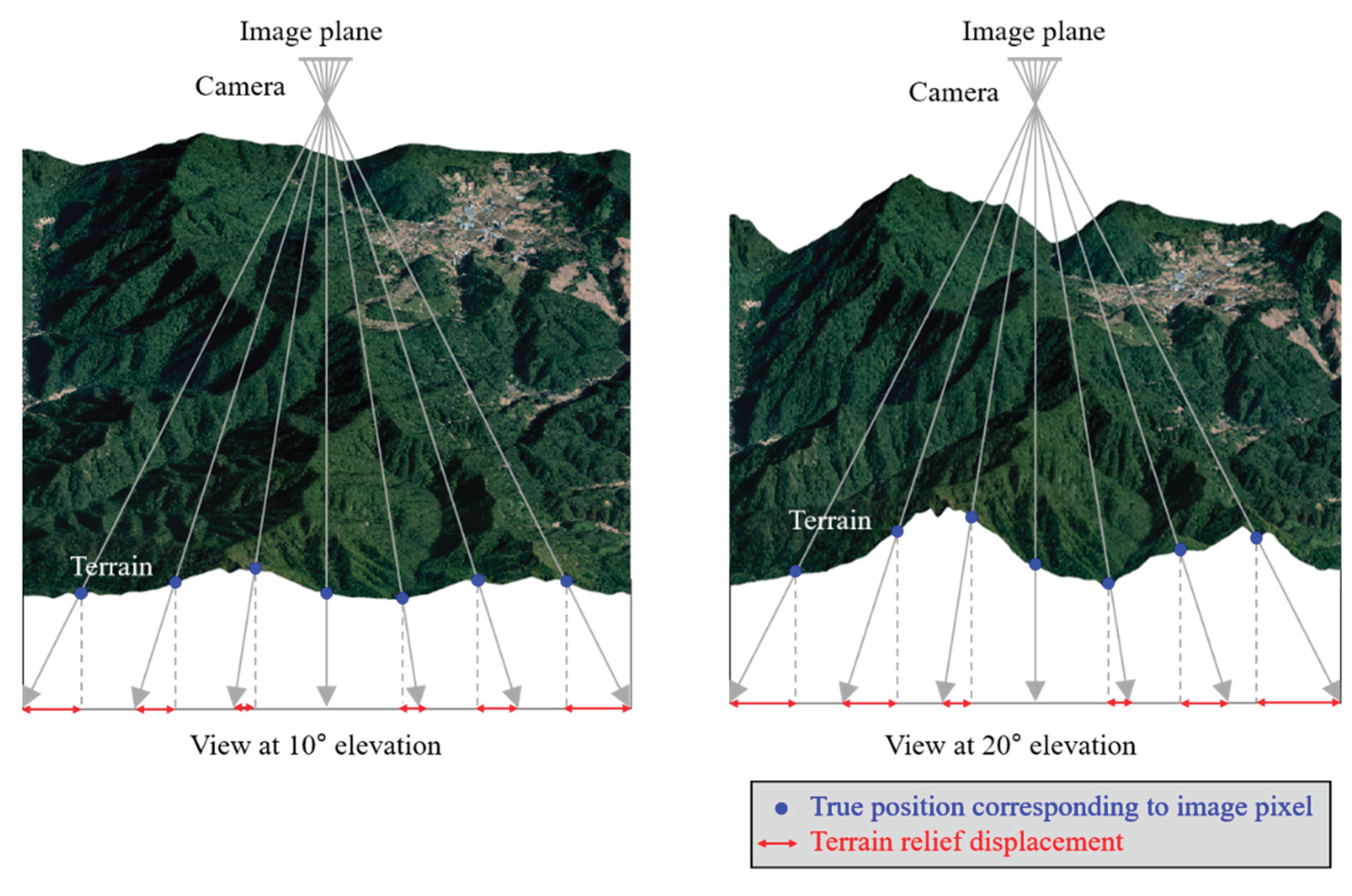
Figure 2.
Block diagram of the proposed VBN algorithm.
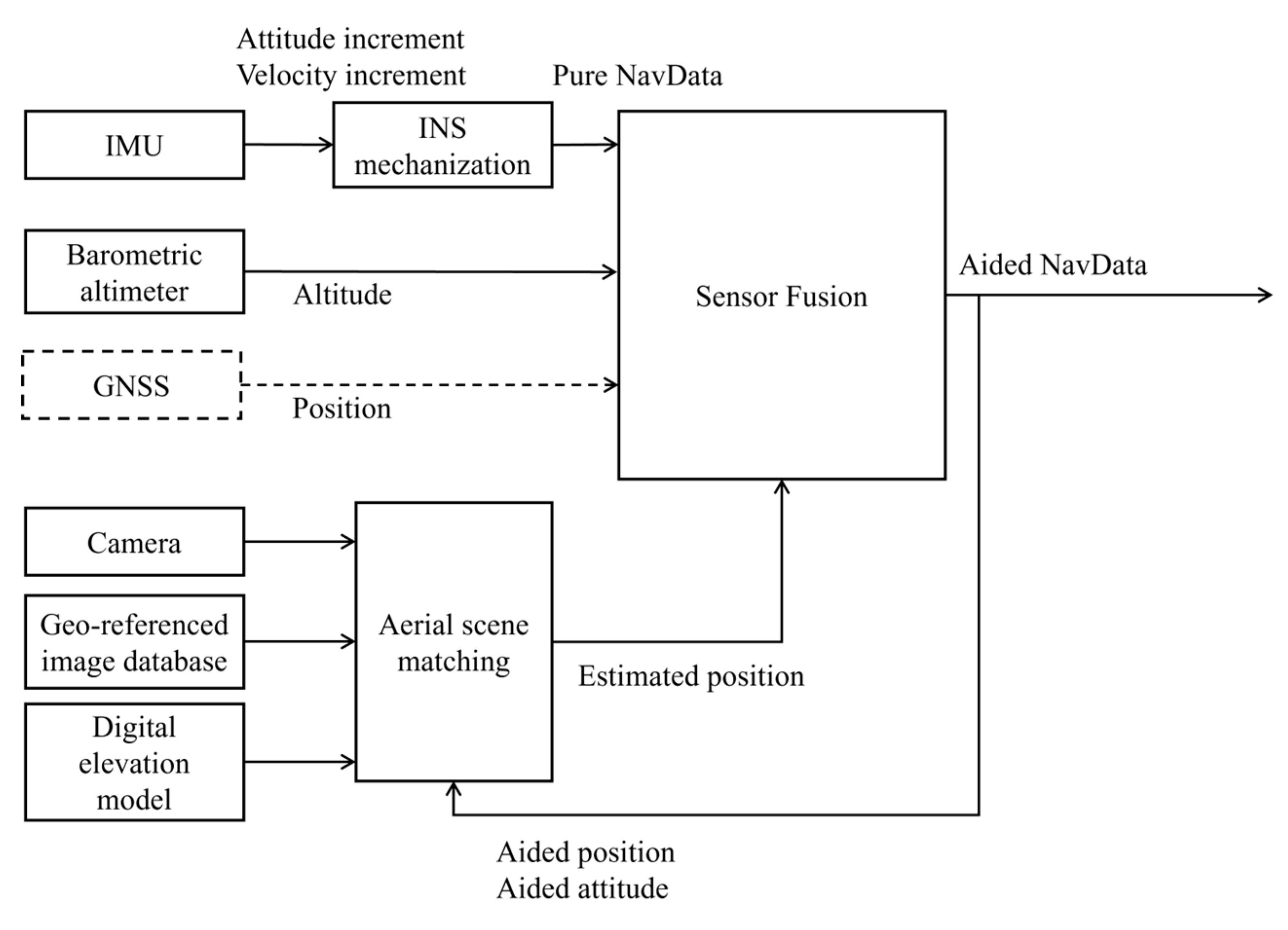
Figure 3.
Flow chart of the proposed SM.
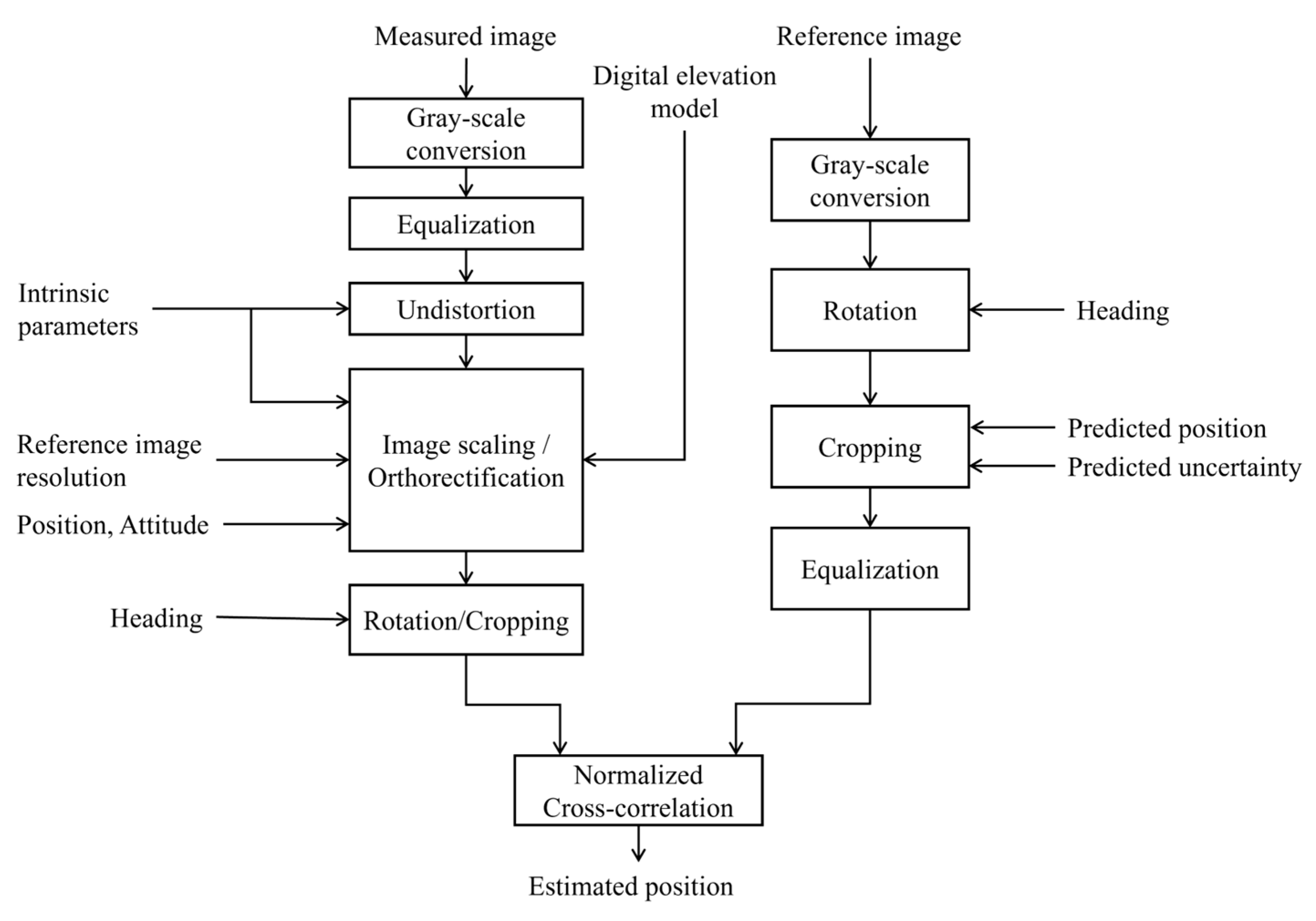
Figure 4.
Simplified 2D representation of the camera projection model for orthorectification. This illustrates a cross-sectional view under the assumption of a pitch angle . Here, denotes the geographic coordinates of the pixel at the -th column and -th row in the camera image plane, and represents the corresponding geographic coordinates of the orthorectified image pixel. is the x- and y-axis coordinates of , and indicates the terrain elevation from the DEM at horizontal position x. The coordinates are determined using an iterative approximation as indicated by the boxed area, where denotes the approximation of at the -th iteration.
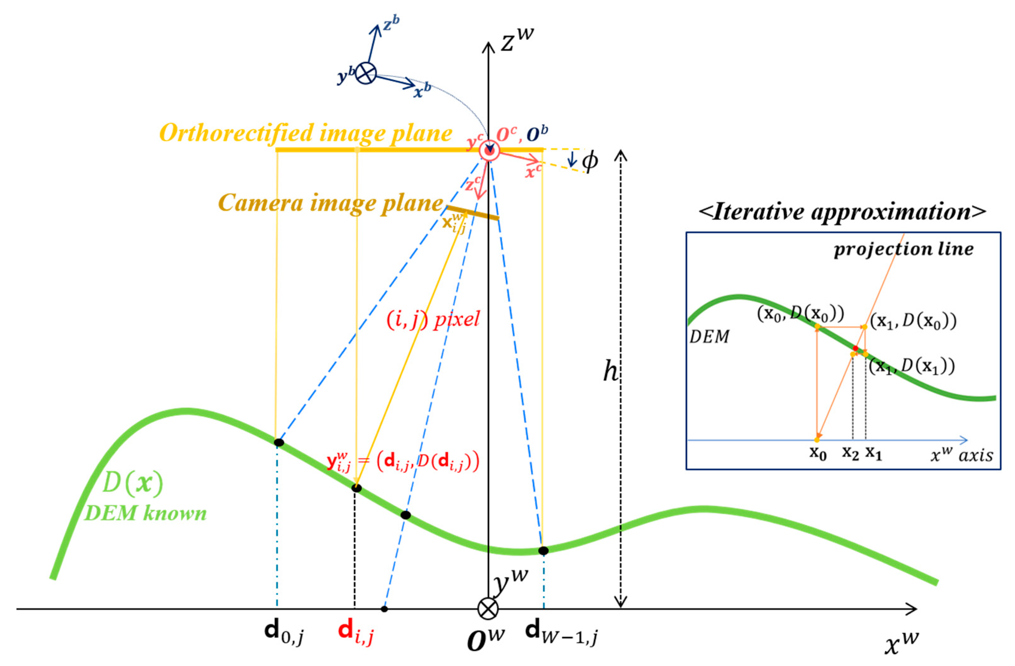
Figure 5.
Results of the orthorectification process. (a) Original aerial image; (b) DEM of the image area; (c) Rectification result with grid; (d) Orthorectification result with grid; (e) Red-cyan composite of (c) and (d) without grid; (f) Difference mask between rectified and orthorectified images with a pixel tolerance of 50; (g) NCC result of the rectified image; (h) NCC result of the orthorectified image.
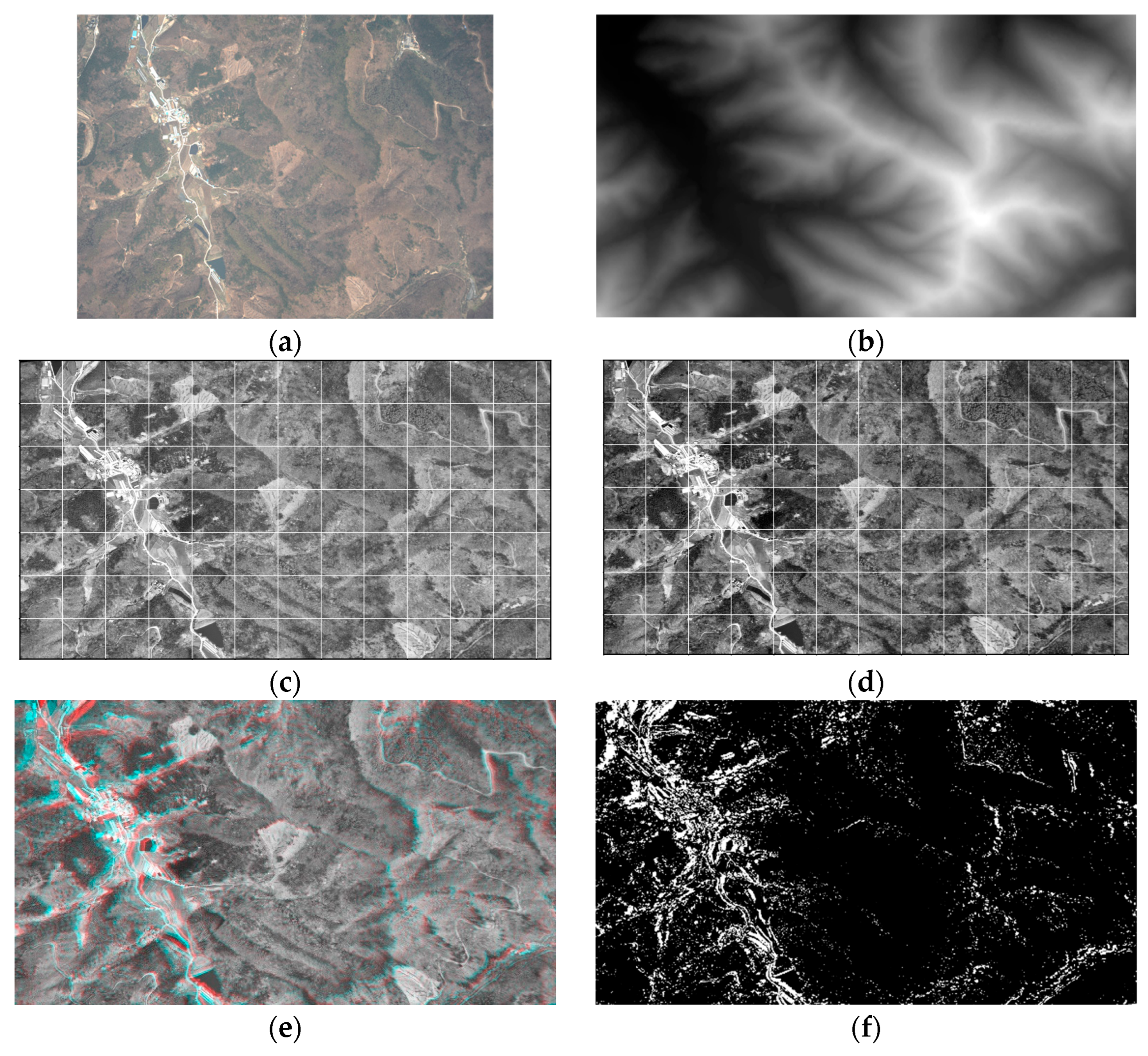
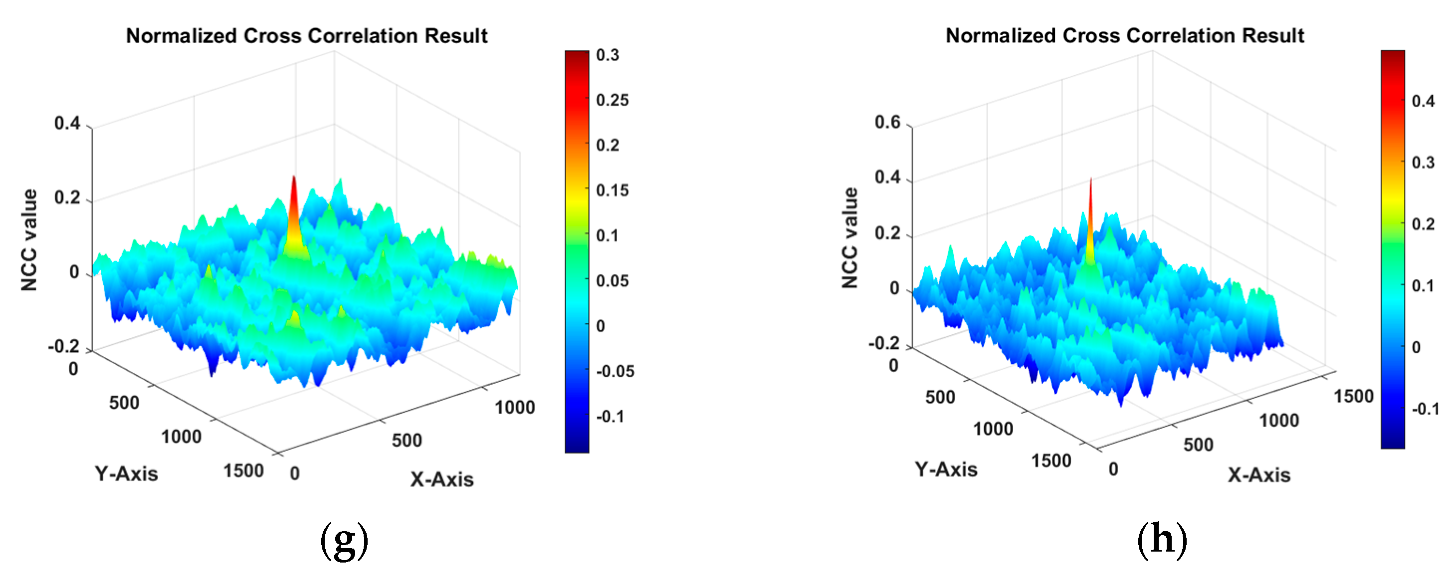
Figure 6.
Sequential results of the signal processing pipeline applied to an aerial image. (a) Equalization; (b) Lens distortion correction; (c) Orthorectification using the proposed method; (d) Final image after rotational alignment and cropping.
Figure 6.
Sequential results of the signal processing pipeline applied to an aerial image. (a) Equalization; (b) Lens distortion correction; (c) Orthorectification using the proposed method; (d) Final image after rotational alignment and cropping.
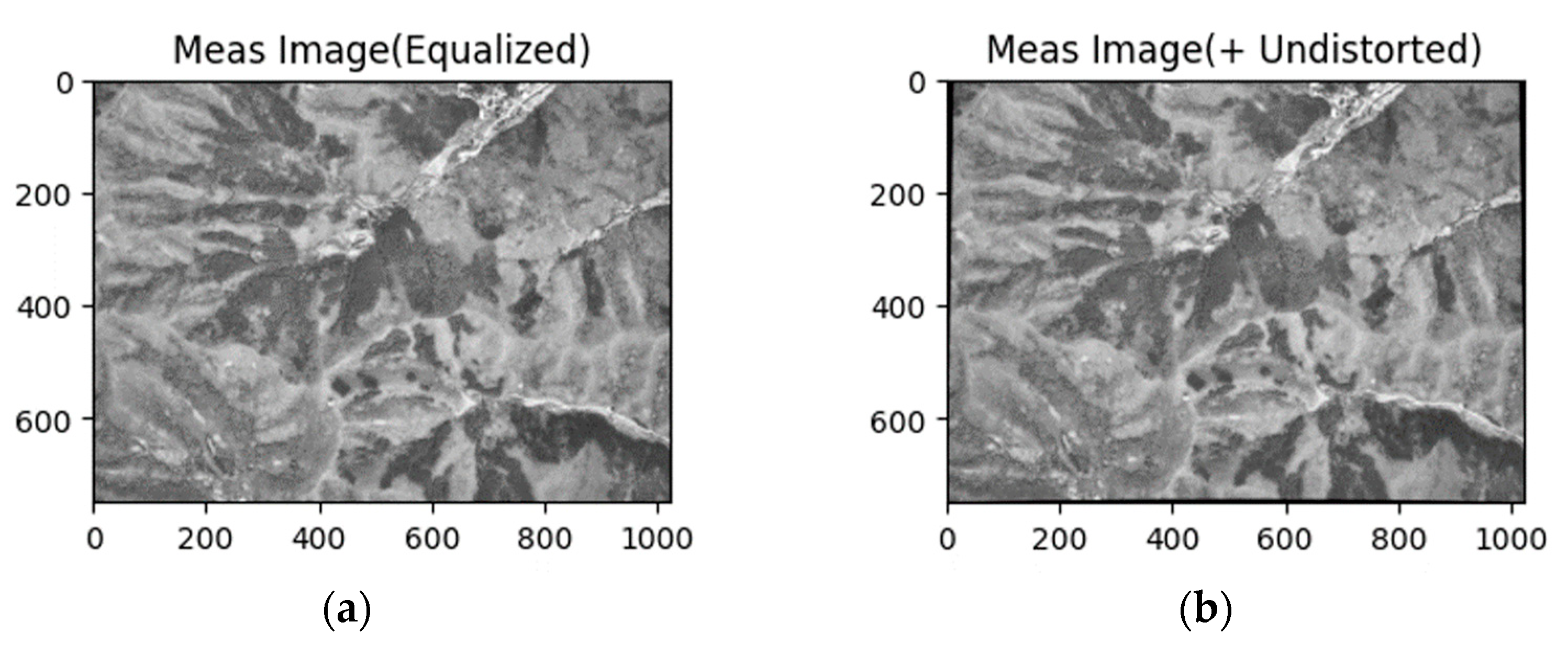
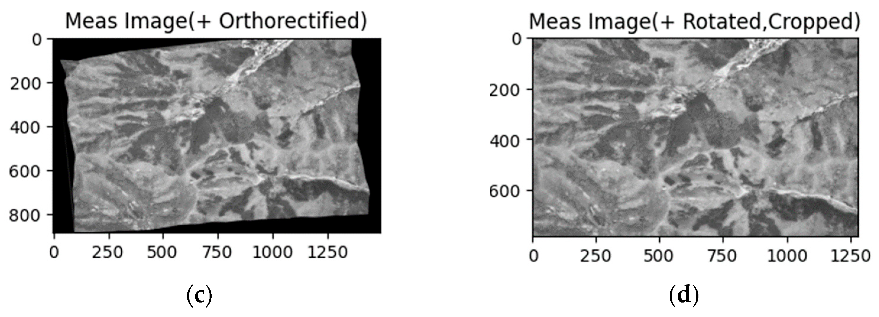
Figure 7.
Block diagram of the proposed sensor fusion framework. The system consists of three components: (i) a horizontal channel EKF that fuses INS outputs with GNSS or SM measurements, (ii) a vertical channel EKF that stabilizes altitude using GNSS or barometric altitude, and (iii) a barometric error estimator that corrects bias and scale-factor error to ensure consistency with the WGS-84 reference. GNSS inputs are represented by dashed lines, highlighting the fallback to SM measurements in GNSS-denied environments.
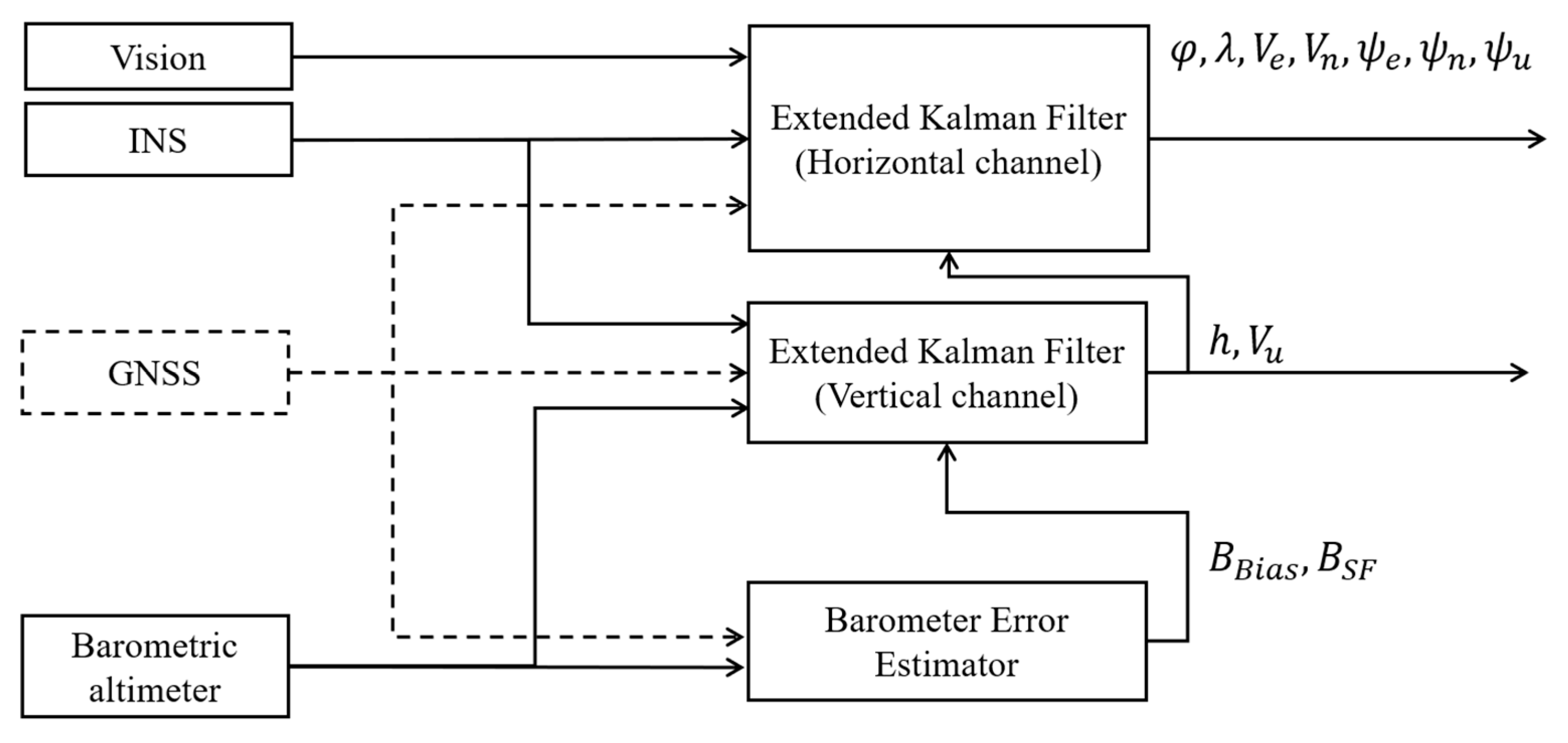
Figure 8.
Aircraft used for flight testing, showing onboard sensors (IMU, GNSS receiver, camera, barometric altimeter)
Figure 8.
Aircraft used for flight testing, showing onboard sensors (IMU, GNSS receiver, camera, barometric altimeter)
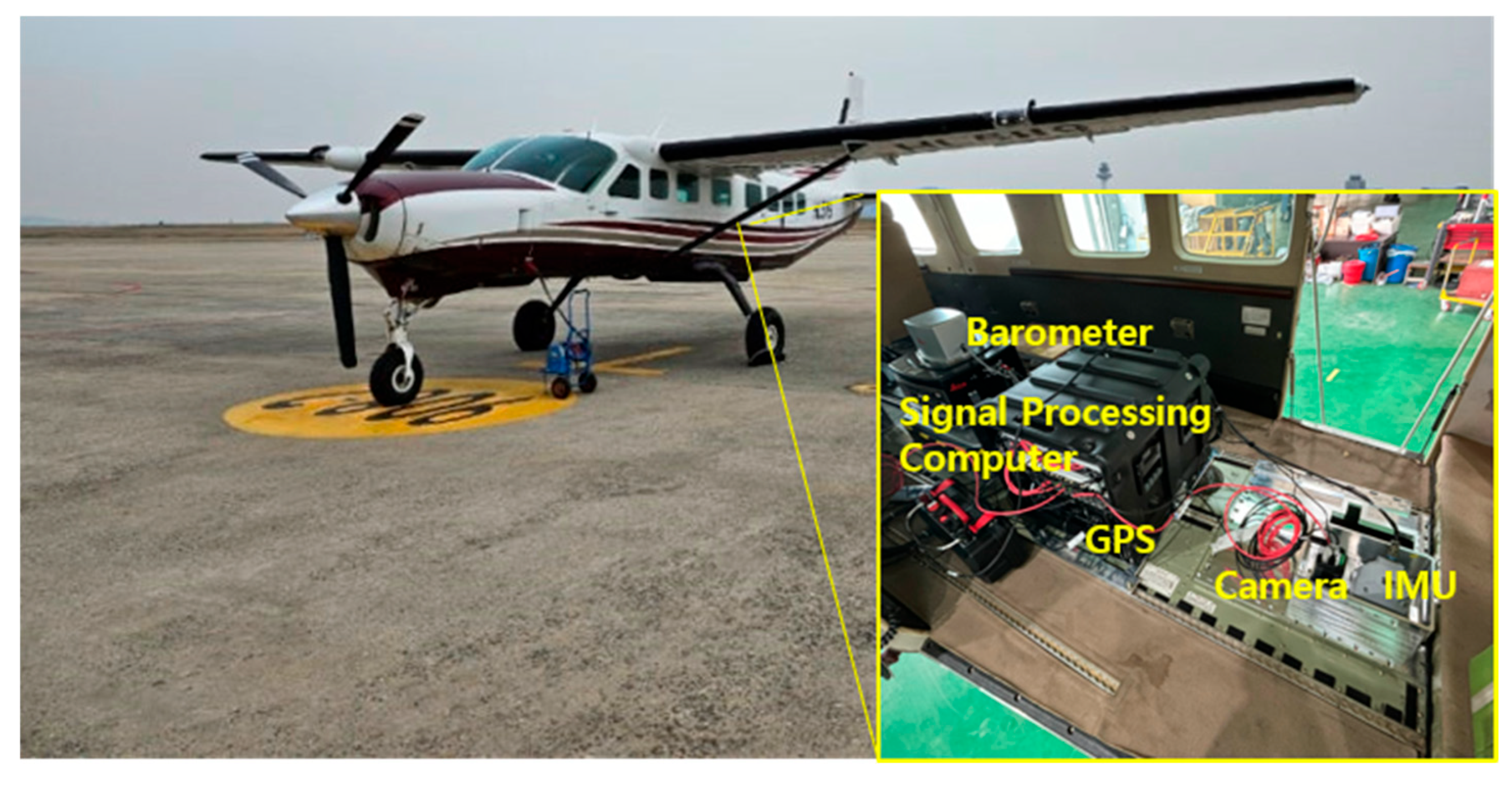
Figure 9.
Flight trajectory information. (a) Georeferenced map of the test area; (b) DEM of the terrain; (c) Terrain elevation profile along Flight Path 2 and 4.
Figure 9.
Flight trajectory information. (a) Georeferenced map of the test area; (b) DEM of the terrain; (c) Terrain elevation profile along Flight Path 2 and 4.
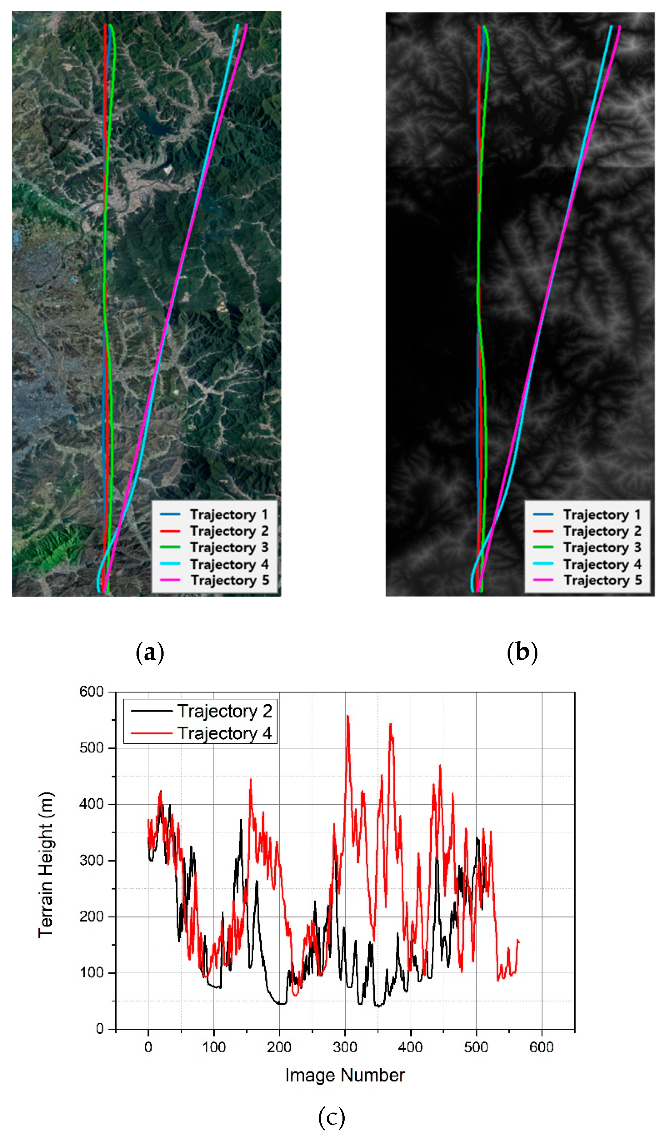
Figure 10.
Horizontal localization error along Flight Path 2 obtained from SM. (a) Results using rectified (Rect.) aerial images; (b) Results using orthorectified (Ortho.) aerial images. Errors are compared under different reference map resolutions: black–8 m, red–4 m, and green–2 m.
Figure 10.
Horizontal localization error along Flight Path 2 obtained from SM. (a) Results using rectified (Rect.) aerial images; (b) Results using orthorectified (Ortho.) aerial images. Errors are compared under different reference map resolutions: black–8 m, red–4 m, and green–2 m.
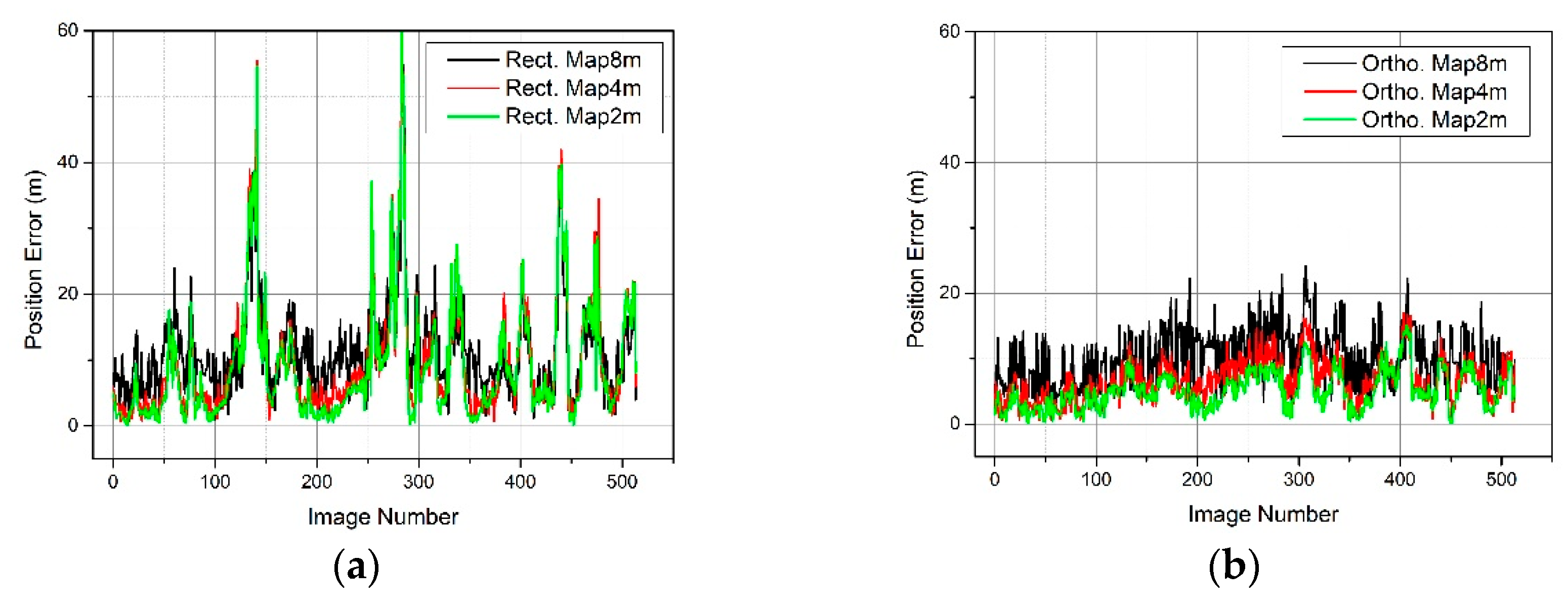
Figure 11.
Graphical representation of localization accuracy from Table 3. (a) 2D RMSE for rectification; (b) 2D RMSE for orthorectification.
Figure 11.
Graphical representation of localization accuracy from Table 3. (a) 2D RMSE for rectification; (b) 2D RMSE for orthorectification.
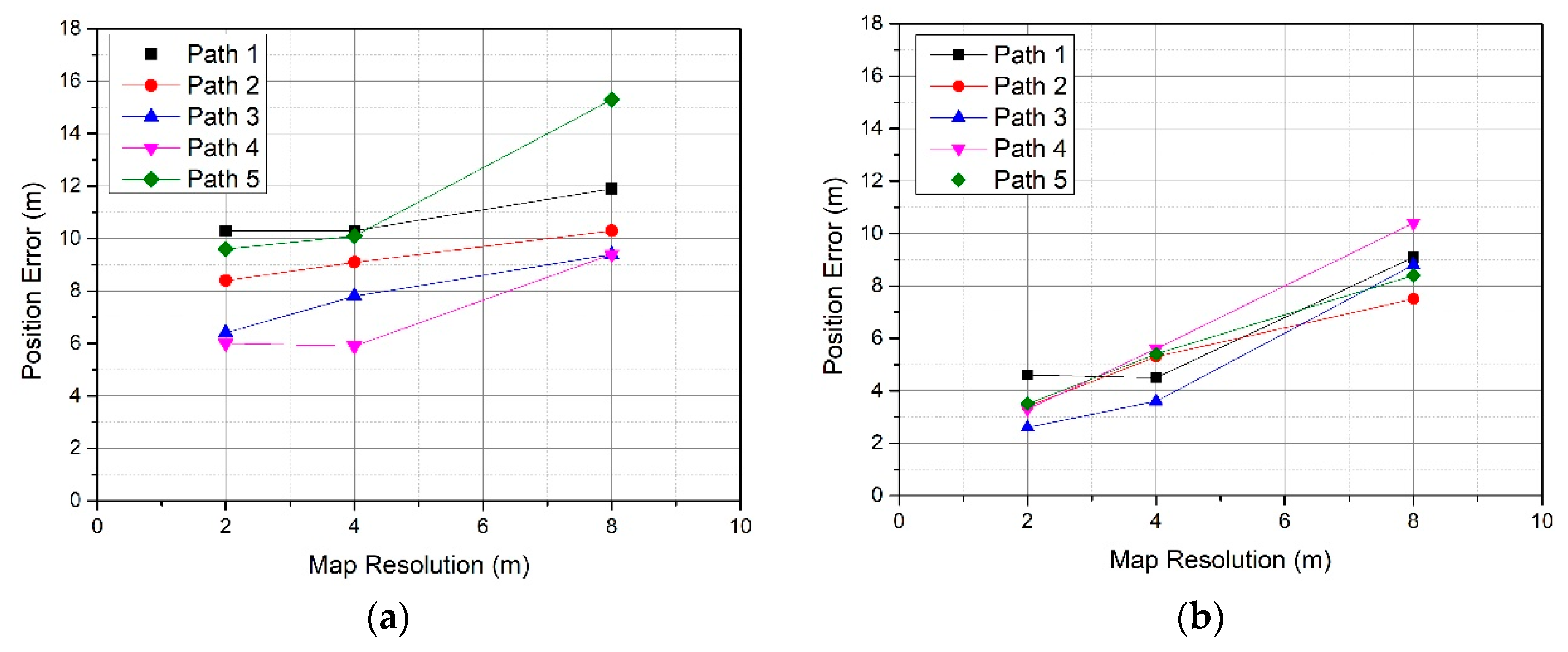
Figure 12.
Horizontal navigation error along Flight Path 2 under GNSS-denied condition using a 4 m resolution reference map. The black line indicates pure inertial navigation; the red line represents VBN with conventional rectification; the green line shows the proposed VBN with orthorectification.
Figure 12.
Horizontal navigation error along Flight Path 2 under GNSS-denied condition using a 4 m resolution reference map. The black line indicates pure inertial navigation; the red line represents VBN with conventional rectification; the green line shows the proposed VBN with orthorectification.
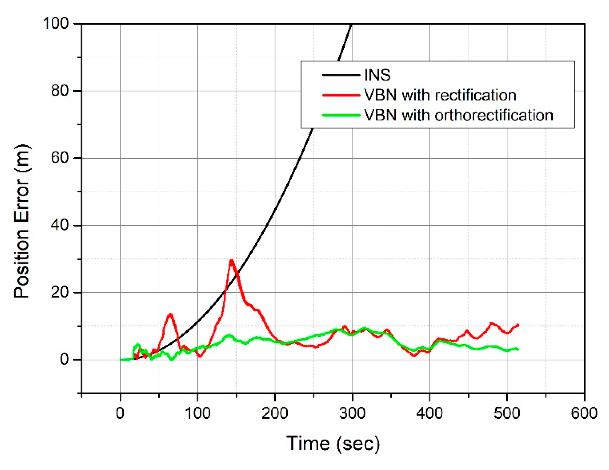
Figure 13.
Horizontal position error along Flight Path 2 using a 4m resolution reference map. (a) Results of the proposed SM with orthorectification (Ortho.); (b) Results of SM with conventional rectification (Rect.). In both subfigures, the black line represents the normal case with minimal navigation errors. While the red, green, and blue lines correspond to navigation error cases 1,2, and 3, respectively, as defined in Table 4.
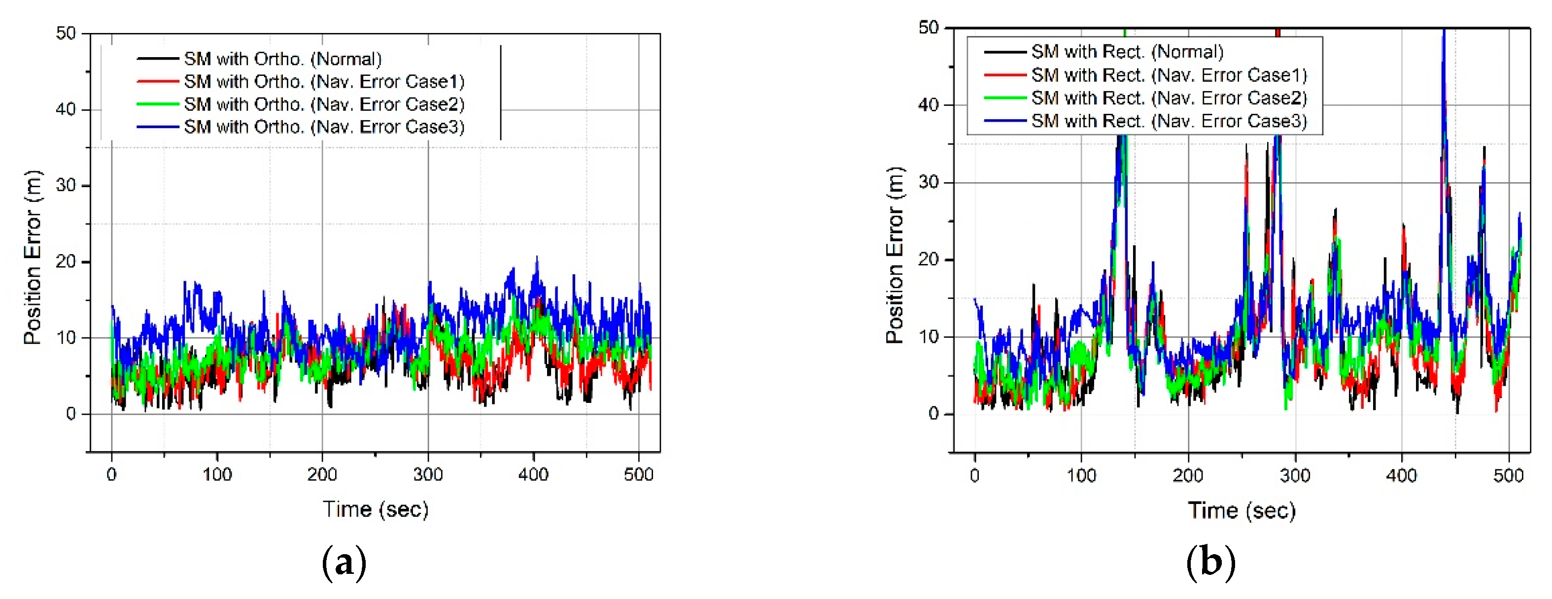
Table 1.
Characteristics of the onboard sensors used in the flight tests
| Sensor | Output rate | Resolution | Bias |
|---|---|---|---|
| Camera | 1 Hz | 4096 × 3000 pixels* | — |
| Gyroscope | 300 Hz | — | 0.04°/h |
| Accelerometer | 300 Hz | — | 60 µg |
| Barometer | 5 Hz | — | — |
* The aerial imagery was downsampled by a factor of ¼ to create an image dataset of 1024x750 pixels.
Table 2.
Flight dataset characteristics for different trajectories.
| Path ID | Heading (°) |
Altitude (km) |
Duration (min) |
Length (km) |
Speed (km/h) |
GSD (m) |
|---|---|---|---|---|---|---|
| 1 | -172.9 | 3.5 | 8.7 | 44.5 | 304 | 2.3 |
| 2 | -8.4 | 3.5 | 8.5 | 44.6 | 311 | 2.3 |
| 3 | -176.9 | 2.5 | 8.9 | 44.6 | 300 | 1.5 |
| 4 | 6.6 | 2.5 | 9.4 | 45.4 | 289 | 1.5 |
| 5 | -165.4 | 2.5 | 9.8 | 45.4 | 278 | 1.5 |
Table 3.
Localization accuracy summarized by 2D RMSE for rectification (Rect.) and orthorectification (Ortho.) across different map resolutions (2, 4, and 8 m) and flight paths (Path ID 1–5).
Table 3.
Localization accuracy summarized by 2D RMSE for rectification (Rect.) and orthorectification (Ortho.) across different map resolutions (2, 4, and 8 m) and flight paths (Path ID 1–5).
| Path ID | Rect. 8m | Rect. 4m | Rect. 2m | Ortho. 8m | Ortho. 4m | Ortho. 2m |
|---|---|---|---|---|---|---|
| 1 | 11.9 | 10.3 | 10.3 | 9.1 | 4.5 | 4.6 |
| 2 | 10.3 | 9.1 | 8.4 | 7.5 | 5.3 | 3.4 |
| 3 | 9.4 | 7.8 | 6.4 | 8.8 | 3.6 | 2.6 |
| 4 | 9.4 | 5.9 | 6.0 | 10.4 | 5.6 | 3.4 |
| 5 | 15.3 | 10.1 | 9.6 | 8.4 | 5.4 | 3.5 |
Table 4.
Simulation cases for SM performance under navigation errors
| Case | Roll/Pitch Error (°) |
Yaw Error (°) |
Latitude/Longitude Error (m) |
Altitude Error (m) |
|---|---|---|---|---|
| 1 | 0.03 | 0.5 | 10 | 20 |
| 2 | 0.05 | 1 | 20 | 40 |
| 3 | 0.1 | 1.5 | 30 | 60 |
Table 5.
VBN localization accuracy for navigation error cases
| Case | 2D RMSE (m) | |
|---|---|---|
| VBN with orthorectification | VBN with rectification | |
| Normal | 5.32 | 9.08 |
| 1 | 5.52 | 9.40 |
| 2 | 6.58 | 9.19 |
| 3 | 9.97 | 10.80 |
Disclaimer/Publisher’s Note: The statements, opinions and data contained in all publications are solely those of the individual author(s) and contributor(s) and not of MDPI and/or the editor(s). MDPI and/or the editor(s) disclaim responsibility for any injury to people or property resulting from any ideas, methods, instructions or products referred to in the content. |
© 2025 by the authors. Licensee MDPI, Basel, Switzerland. This article is an open access article distributed under the terms and conditions of the Creative Commons Attribution (CC BY) license (https://creativecommons.org/licenses/by/4.0/).
Copyright: This open access article is published under a Creative Commons CC BY 4.0 license, which permit the free download, distribution, and reuse, provided that the author and preprint are cited in any reuse.


