

Submitted:
09 September 2025
Posted:
09 September 2025
You are already at the latest version
Abstract
Many problems in science, engineering, and economics require solving nonlinear equations, often arising from attempts to model natural systems and predict their behavior. In this context, iterative methods provide an effective approach to approximate the roots of nonlinear functions. This work introduces five new parametric families of multipoint iterative methods specifically designed for solving nonlinear equations. Each family is built upon a two-step scheme: the first step applies the classical Newton method, while the second incorporates a convex mean, a weight function, and a frozen derivative (i.e., the same derivative from the previous step). The careful design of the weight function was essential to ensure fourth-order convergence while allowing arbitrary parameter values. The proposed methods are theoretically analyzed and dynamically characterized using tools such as stability surfaces, parameter planes, and dynamical planes on the Riemann sphere. These analyses reveal regions of stability and divergence, helping identify suitable parameter values that guarantee convergence to the root. Numerical experiments confirm the robustness and efficiency of the methods, often surpassing classical approaches in terms of convergence speed and accuracy. Overall, the results demonstrate that convex-mean-based parametric methods offer a flexible and stable framework for the reliable numerical solution of nonlinear equations.
Keywords:
iterative methods
; nonlinear equations
; convergence order
; optimal methods
; dynamical analysis
1. Introduction
In mathematics and engineering, many real-world and physical phenomena are modeled using nonlinear equations or systems. Solving such problems has led to the development of numerous numerical methods, which serve as fundamental tools for approximating solutions that cannot be found exactly or analytically.
Among these, iterative methods play a crucial role in finding the roots of nonlinear equations. Since a variety of iterative strategies exist, it becomes essential to evaluate their convergence order, stability, and computational efficiency. These aspects allow us to compare methods and choose the most appropriate one for a given problem.
Iterative methods are typically classified based on whether they are single-step or multi-step, with or without memory, and whether they require derivatives or not . In this context, we present new multipoint iterative methods aimed at approximating the zeros of nonlinear functions. These methods are inspired by the work in [1], which investigates and enhances Newton-type methods by incorporating convex combinations of classical means, achieving third-order convergence.
With the aim of improving this order of convergence, we introduce new multipoint iterative schemes based on the composition and in the use of weight function. These functions combine data from multiple evaluations of the function and its derivatives throughout previous iterations to improve both accuracy and efficiency. The proposed methods achieve fourth-order convergence and satisfy the optimality condition postulated by the Kung-Traub conjecture [2], which states:
The order of convergence p of a without memory iterative method cannot exceed , where d is the number of functional evaluations per iteration.
A method that reaches this bound is called optimal. This and other criteria described below will allow us to define which method is more effective than another.
One of the most widely used and foundational approaches in nonlinear root-finding is Newton’s method. It is defined as:
provided . Under appropriate smoothness conditions and for simple roots, the method exhibits quadratic convergence, meaning:
for some constant and being a root of .
In 2000, Weerakoon and Fernando [3] proposed a third-order variant of Newton’s method. This method replaces the rectangular approximation in the integral form of Newton’s method with a trapezoidal approximation, reducing truncation error and improving convergence. Their method, known as the trapezoidal or arithmetic mean method, is defined as:
This method laid the foundation for subsequent generalizations using other types of means. Researchers such as Chicharro et al. [4] and Cordero et al. [1] expanded this idea by incorporating various mathematical means to construct families of third-order methods:
where denotes the Newton step and represents the chosen mean applied to the values x and y.
1.1. Types of Means
Below are the different types of convex averages used in the literature for the design and analysis of various iterative methods. These concepts constitute a fundamental reference and will serve as a methodological basis for the development of our own iterative procedures.
Arithmetic Mean : The arithmetic mean of two real numbers x and y is given by:
This mean appears in the trapezoidal scheme (2).
Harmonic Mean : The harmonic mean of two positive real numbers x and y is defined as:
This mean is particularly sensitive to small values and is known for its use in rates and resistances. In the context of iterative methods, its reciprocal nature often yields improved stability under specific conditions. The following scheme arises by replacing in (2) the arithmetic mean by this mean, as done in [5]:
Contraharmonic Mean : The contraharmonic mean is given by:
and is always greater than or equal to the arithmetic mean. It accentuates larger values, making it suitable when higher magnitudes dominate the behavior of the function. When this mean is incorporated into iterative schemes, the obtained method presented in [1,6] is:
Different authors have proved that all these schemes have order of convergence three.
1.2. Some Characteristics of the Iterative Methods
To analyze an iterative method in greater depth, it is essential to understand certain concepts related to the mathematical notation used, the order of convergence, the efficiency index, the computational order of convergence, as well as the fundamental theorems and conjectures that support the correct formulation of the proposed new multipoint methods. Each of these aspects is detailed below.
Order of convergence
The speed at which a sequence approaches a solution is quantified by the order of convergence p. Formally, the sequence is said to converge to with order and asymptotic error constant if:
This limit establishes an asymptotic relation that describes how rapidly the errors decay as the number of iterations increases. Specifically:
- If and , the convergence is linear,
- If , the convergence is quadratic,
- If , the convergence is cubic,
- For , the method has higher-order convergence.
In practice, a high value of p implies faster convergence toward the root of , assuming the constant C remains reasonably small. However, higher-order methods often require more function or derivative evaluations per iteration, increasing computational cost.
The error equation of an iterative method can be expressed as:
where C is the asymptotic error constant and denotes higher-order terms that become negligible as n increases. This expression is central to the local convergence analysis of iterative schemes.
Numerical estimation of the order of convergence
Since the exact root is typically unknown, practical estimation of the convergence order relies on approximate values of the iterates. Two widely used techniques are:
These tools are commonly used in numerical experimentation to assess the performance of iterative schemes.
The classical estimate (COC) [3], assuming knowledge of the root , is given by:
When is unknown, the ACOC [7] formula provides a root-free estimate using only the iterates:
This tool allows us to approximate the theoretical order of convergence p without requiring knowledge of the exact solution. Its reliability increases as the iterates approach the root, provided the errors remain sufficiently small to avoid numerical cancellation or round-off issues.
Efficiency Index of an Iterative Method
To assess the computational efficiency of an iterative method, one must consider its convergence order and the number of function evaluations per iteration. Ostrowski (1966) introduced the efficiency index I, defined as:
where p is the order of convergence and d is the total number of functional evaluations per iteration (including derivatives, if applicable). This index provides a comparative efficiency measure across methods with varying orders and computational demands.
More recently, the concept has been extended to the computational efficiency index (CEI) [8], which includes not only functional evaluations but also the products/quotients of the iterative method.
where refers to the number of products/quotients produced in each iteration.
These indicators allow different iterative methods to be compared regarding convergence speed and total computational cost.
In this manuscript, Section 2 presents some known fourth-order iterative methods used in the numerical section for comparison. In Section 3, the new schemes are presented and their order of convergence is proven. Section 4 deals with the dynamical analysis of one of the proposed families of iterative schemes. The best method in terms of stability is compared in the numerical section with known schemes. Two academic examples and two applied problems confirm the theoretical results. With some conclusions and references, we conclude the manuscript.
2. Some Fourth-Order Methods in the Literature
In recent decades, there has been an urgent need to develop iterative methods with high orders of convergence that do not require new functional evaluations or derivatives. Since Traub’s initial contributions [9] with his method known as the frozen derivative, various approaches have been proposed to address this challenge. The following iterative expression defines Traub’s method:
This scheme achieves cubic convergence without the need to evaluate the second derivative. Similarly, Jarratt [10] introduced a two-step iterative scheme:
This also avoids evaluating second derivatives and achieves fourth-order convergence.
Based on these ideas, many multipoint methods have been developed to achieve even higher convergence orders. The specialized literature, including the works of Chun [11], Ostrowski [12], King [13], among others, offers a wide range of fourth-order schemes based on the adjustment of parameters and weighting functions. These schemes will serve as benchmarks for comparison with the methods proposed in this work.
Among them, it is worth highlighting the family of fourth-order methods introduced by Artidiello [14]. It is based on a weighting function that generalizes several known schemes. Its formulation follows a two-step scheme:
where .
Theorem 1
([14]). Let be a sufficiently differentiable function on an open interval I containing a simple root α of , and any sufficiently differentiable function satisfying:
Then, for an initial estimate close enough to α, method (7) converges with order at least 4 and its error equation is:
where and .
This theoretical framework not only unifies classical methods (such as those of Ostrowski or Chun) through specific choices of , but also provides a rigorous basis for designing new schemes. Table 1 summarizes several iterative methods that achieve fourth order thanks to the correct consideration of weighting functions.
Each of these weight functions iterative methods satisfies the conditions , achieving the corresponding scheme a fouth-order convergence.
3. General Framework of Mean-Based Iterative Methods
As mentioned in the SubSection 1.1, all iterative methods exhibit cubic convergence. Consequently, this motivates the creation of a new family of iterative methods in which weight functions play a key role in increasing the order of convergence from three to four, without adding new functional evaluations.
We consider the following multipoint method:
where represents the Newton step, is an arbitrary mean applied to and , and is a weight function, with .
By choosing different symmetric means , such as: the arithmetic mean () and (); the harmonic mean (); the counterharmonic mean () and (), we obtain several iterative schemes with different correction steps, as summarized in Table 2.
Theorem 2
Let be a sufficiently differentiable function on an open interval I, holding its simple root , that is, and . The multipoint iterative method defined by a Newton step:
followed by a corrector step
where:
- is a symmetric bivariate function representing a mean (, , , or ),
- , is the variable of the weight funtion H,
- is a weight function with a Taylor expansion around :
If the coefficients satisfy specific conditions given in Table 3 then the method achieves fourth-order convergence.
All methods achieve fourth-order convergence, with the generalized error equation:
and represents the iteration error. The constants and depend on the chosen mean and on the coefficients of the weight function .
Proof.
Let denote the error at the n-th iteration. Since f is sufficiently differentiable and is a simple root, we can use Taylor expansions of and around . In terms of , we have:
Since , it follows that
We simplify the calculations using the expression of the constants (11)
In a similar way,
Therefore,
So,
Hence, the error in the approximation of becomes:
In terms of , we obtain:
Therefore,
We calculate, by direct division,
Since as , we expand the weight function in a Taylor series around :
Substituting the expression in terms of , we obtain:
Now, we detail the expansion of using the arithmetic mean of Table 2. For the rest of the means, all calculations are analogous.
Thus, equation of Table 2 expands to:
that is,
By solving the system obtained from eliminating the first-, second, and third-order error terms, ensuring that:
the error of the method based on the arithmetic mean becomes:
This finishes the proof for the case of the arithmetic mean. The order of convergence of the remaining methods is obtained in a similar way, replacing the mean function and using the corresponding values of the coefficients of presented in Table 3. Proceeding in this manner, the methods indicated in Table 2 achieve a fourth-order convergence. □
4. Dynamical Analysis
The order of convergence of an iterative method is not the only relevant criterion when evaluating its performance. In fact, the dynamical of the method, that is, the behavior of its orbits under different initial estimations, plays a fundamental role in its overall analysis. For it, tools from complex analysis are used, which represent the evolution of the methods in the Riemann sphere [17,18,19].
We start from a rational function resulting from the application of an iterative method to a polynomial of low degree, denoted by , where denotes the Riemann sphere. The orbit of a point is given by the sequence:
We are interested in studying the asymptotic behavior of the orbits, so we must classify the different points of the rational operator R. A point is k-periodic , if
We say that it is a fixed point of R if
If this fixed point is not a solution of the polynomial, it is called a strange fixed point, as well as being numerically undesirable, since the iterative method can converge on them under certain initial guesses [18].
The dynamical behavior of these fixed points is classified according to the modulus of the derivative . If , the fixed point is an attractor; if , it is called parabolic or indifferent; if , it is repellent; and if , it is a superattractor.
On the other hand, the study of the basin of attraction of an attractor is defined as the set of points that converge to it
The Fatou set F is the union of the basins of attraction. The Julia set J is its topological complement in the Riemann sphere and represents the union of the frontiers of the basins of attraction.
The following classic result, given by Fatou [20] and Julia [21], includes both periodic points (of any period) and fixed points, considered as periodic points of unit period.
Theorem 3
Let R be a rational function. The immediate basins of attraction of each attractive periodic point contain at least one critical point.
Using this key result, the entire attraction behavior can be found using the critical points as seeds of the iterative process [22]. A point is critical for R if:
We are going to start with a rational function resulting from the application of an iterative scheme on a quadratic polynomial. In order to obtain global results for the class of quadratic polynomial we prove a Scaling Theorem for the corresponding iterative method.
4.1. Conjugacy Classes
Let f and g be two analytic functions defined on the Riemann sphere. An analytic conjugacy between f and g is a diffeomorphism h on the Riemann sphere such that .
We now state a general theorem that applies to all types of symmetric means described in Table 2.
Theorem 4
Let be an analytic function on the Riemann sphere, and let be an affine transformation with , and , with . Let us consider the iterative scheme defined by
where is Newton’s method, being one of the means that provide the schemes , , or , , Here, satisfies the conditions indicated in Table 3.
Then, (19) is analytically conjugate to the analogous method applied to g, that is:
sharing the same essential dynamics.
Proof.
To prove the general result, we consider a particular case of the mean. For the rest of the methods, the proof is analogous. We choose the case of , whose scheme is given by:
As can be seen, its structure is representative of the methods included in Table 2. We know that the affine function has an inverse given by .
By hypothesis, . By the chain rule, we obtain:
Defining the operator as
and evaluated at , we obtain:
Using the identities from (22) and taking into account that
we deduce that:
Now, we apply the transformation h:
We observe that the term transforms as:
The same reasoning extends directly to the methods in Table 2, since:
- In each case, the correction term maintains the form , with symmetric combinations based on means.
- The affine transformation h acts compatibly on both and , preserving the functional structure of the correction.
- The identity holds, since it depends only on the ratio , scaled by .
Therefore, the result holds for the entire family of iterative methods based on symmetric means, as described in Table 2.
4.2. Dynamics of Fourth-Order Methods
As shown in Table 2, five different parametric families of iterative methods are identified, each of them associated with specific conditions on the function . To satisfy these conditions, polynomial weight functions have been selected. However, other types of functions could also be considered, as long as they meet the imposed constraints. This also allows the introduction of an additional parameter in cases where is bounded.
Table 4 presents the polynomials chosen by the authors for the development of this paper.
Here, and is a free parameter.
To observe the dynamics of these iterative methods, we will take as an example the arithmetic mean family , which is defined as:
The other cases can be analyzed in a similar way.
4.3. Rational Operator
Proposition 1.
Let us consider the generic quadratic polynomial , of roots a and b. The rational operator related to family given in (28) on is:
being an arbitrary parameter.
Proof.
We apply the iterative scheme to and obtain a rational function that depends on the roots and the parameter . Then, we apply a Möbius transformation [19,23,24] on with
which satisfies and . This transformation maps the roots a and b to the points 0 and ∞, respectively, whose nature is attractive, and the divergence of the method to 1. Thus, the new conjugate rational operator is defined as:
which no longer depends on the parameters a and b. □
Thus, this transformation facilitates the analysis of the dynamics of iterative methods by allowing the standardization of roots and the structural study of dynamic planes and their stability regions [8].
4.4. Fixed Points of the Operator
Now, we calculate all the fixed points of , to subsequently analyze their character (attractive, repulsive, neutral, or parabolic). Taking into account that the method has order four, the points and are always superattractor fixed points, since they come from the roots of the polynomial.
The fixed points of are , , and nine strange fixed points:
- is a strange fixed point if ,
- The roots of the polynomial:denoted by , , for any .
Now, we study the stability of the strange fixed point .
Proposition 2.
The strange fixed point has the following character:
- If , is not a fixed point.
- If , is attractor.
- If , is parabolic.
- If , is repulsive.
Proof.
As seen in the previous section, the behavior of the fixed point can be determined according to the value of the stability function: it will be an attractor if , a repulsor if , superattractor if and parabolic if . The expression of operator is
Therefore,
If , then is not a fixed point. To determine whether it is attractive or repulsive, we solve:
Expressing the right side in terms of and :
So,
By simplifying, we get
thus,
□
Graphically, the behavior of the fixed point is visualized in Mathematica using the graph of the function .
In Figure 1, the attraction zones are the yellow area and the repulsion zone corresponds to the gray area. For values of within the disk, is repulsive; while for values of outside the gray disk, becomes attractive. Therefore, it is natural to select values within the gray disk, since repulsive divergence improves the performance of the iterative scheme.
For the eighth roots , , of polynomial , we obtain the following results:
- , there is no value,
- , for , and ,
- , for , and ,
- , for ,
- , there is no value,
- , for ,
- , for ,
- , for .
In the following figure we represent the stability functions of the strange fixed points points , .
For each root evaluated in the rational derivative operator (), its stability surfaces are constructed. In this context, the graphical representation distinguishes the orange regions as zones of attraction , the gray regions as zones of repulsion , superattraction zones when it is the vertex of the cone , and parabolic zones when it is at the boundary .
From Figure 2, the following conclusions are drawn:
- As the derivative operator associated with the strange fixed points can not be zero, it can be seen in Figure 2 that the resulting surface has only one gray region. This indicates that these fixed points are repulsive throughout the analyzed range, which is desirable, as it prevents convergence to a strange fixed point.
- Furthermore, at points , we obtain we obtain and . Figure 2 shows an inverted cone-shaped surface (normally yellow), representing an attractor inside the cone and a superattractor at its vertex (that of is similar, so it is omitted). The associated unstable domain is approximately , indicating a small but localized region. Similarly, by setting the derivative operator associated with the roots to zero, we obtain and . Figure 2 and Figure 2 show behavior qualitatively similar to that of , with a comparable domain.
- By setting the derivative operator associated with the roots to zero, we obtain . As illustrated in Figure 2, a considerably wider region of attraction appears, approximately , indicating that the method shows marked instability for these values of .
Therefore, to ensure the robustness of the method, values of where some root is an attractor or superattractor should be avoided. In contrast, values such as where all strange fixed points are repellers, are preferable to ensure stable numerical behavior.
Just as we have studied strange fixed points, we must also analyze critical points, since, recalling Theorem 3, it turns out that each attraction basin of an attractive periodic point (any period) contains at least one critical point.
4.5. Critical points of the operator
Proposition 3.
The critical points of the rational operator are , , directly related to the zeros of the polynomial, and the following free critical points:
where the auxiliary functions , , , , and are algebraic simplifications used for easy of notation:
Thus, there are five free critical points, except for , , and , where only three free critical points exist.
Proof.
To prove the result, we recall that the derivative of the rational operator () is:
It is easily observed that its roots are , , , and . These last four correspond to the roots of the polynomial of degree 4 in the numerator.
Now, let us observe that for certain values of , only three free critical points exist. One such case is , where the derivative of the operator simplifies to:
Here, the strange critical points are , and the conjugate pair
When , the derivative operator becomes:
In this scenario, the strange critical points are , and the conjugate pair
And finally, when , the derivative operator becomes:
whose zeros are and the conjugate pair
□
For the free critical point , we have , which is a strange fixed point. Therefore, the parameter plane associated with this critical point is not of much interest, since we already know the stability of .
To visualize the behavior of the free critical points that depend on , we plot the parameter planes. In each parameter plane, we use each free critical point as an initial estimation. A mesh of points is defined in the complex plane. Each point of the mesh corresponds to a value of , that is an iterative method member to the family, and for each one of them, we iterate the rational function . If the orbit of the critical point converges to or in a maximum of 100 iterations, the point is colored red; otherwise, it is colored black.
As a first step, we graph the parameter plane of the conjugate pair , both in the domain , which represents a broad stable performance region around the origin, and , which represents a divergence zone related to the .
It is observed that there are many values of the parameter for which the free critical points converge to the roots or , visually, showing convergence in an approximate domain of . On the other hand, Figure 3 presents a divergence detail and refers to the strange fixed points and , which, when computing their derivative operator set to zero, yielded a value of , which precisely aligns with the divergence observed in Figure 2.
Likewise, the parameter plane of the conjugate pair is shown, both in the domain , and a detail in the domain , which represents the region that has not converged to any of the roots.
4.6. Dynamical Planes
In the case of dynamical planes, each point in the complex plane is considered as a starting point of the iterative scheme and is represented with different colors depending on the point it converges to. In this case, points that converge to are colored blue, and those that converge to are colored orange. These dynamical planes have been generated using a grid of points and a maximum of 100 iterations per point. In these planes, the fixed points are represented by a white circle, the critical points by a white square, and the attracting points by an asterisk.
Next, the dynamical planes are plotted based on the values for obtained from the strange fixed points of the operator () and from the observations in the parameter plane.
In Figure 5 and Figure 6, good behavior of the method can be observed when choosing and . The colors of the plots indicate convergence of the method to and , which are the roots.
A notable case is , since in Proposition Section 4.4 it was established that when takes that value, is not a fixed point, as observed in Figure 7.
In Figure 8, it can be clearly seen that is no longer characterized as a strange fixed point of the method. Moreover, we recall that when , is repulsive, as shown in Figure 5 and Figure 6, and when , is an attractor, as shown in Figure 9 and Figure 10.
Observe that when evaluating the dynamical plane in Figure 9, the method converges to ; a strange fixed point of the rational operator, even though the root is relatively closer. Furthermore, note the notable instability of choosing such a high value of .
Based on the previous study (see Figure 2), when considering the value , complex dynamical behavior was observed. In that figure, it is seen that the associated attraction cone covers a significantly larger area compared to other values of . Additionally, this basin of attraction is related to the parameter plane of the conjugate critical point . In this scenario, the method converges to basins different from the roots 0 and ∞, indicating that it is not suitable for root-finding. Therefore, values such as should be avoided when applying this method. Likewise, another example of divergence .
Figure 11.
.

The analysis of the remaining iterative methods presented in Table 4 has been carried out similarly. The same qualitative information obtained in the previous analysis was also found in the rest of the families. The union of parameter planes is the same for all families. Therefore, their qualitative performance is the same, with a wide area of complex values for parameter giving rise to stable methods.
5. Numerical Examples
The iterative methods used in this section are presented in Table 4. This table considers all the conditions established in Table 3 with respect to , aiming to guarantee fourth-order convergence. In particular, the parameter is selected, given its favorable behavior observed in the dynamical analysis.
To assess the efficiency of the newly proposed iterative methods, a comparison is made with classical algorithms from the literature, as listed in Table 1.
This section evaluates the performance of the newly proposed multipoint iterative methods compared to several well-established fourth-order methods. The comparison includes the following performance indicators:
- Number of iterations required for convergence (Iter),
- Approximate Computational Order of Convergence (ACOC),
- Bounds of the errors (Incr, Incr2), where
- Efficiency Index (EI),
- Execution time (Time), measured in seconds.
5.1. Academic Example 1:
The target root of the problem considered is , obtained from the proposed nonlinear function. For the iterative process, was taken as the initial estimate, with a convergence tolerance of and a maximum number of 100 iterations. The implemented algorithm uses as a stopping criterion.
If neither criterion is met, the procedure ends when the maximum number of iterations is reached. Table 5 presents the results obtained under these conditions.
The results reported in Table 5 underscore the strong competitiveness of the newly developed methods when compared with classical schemes. The proposed approaches exhibit comparable, and in several cases superior, performance in terms of both accuracy and computational efficiency. This is reflected not only in the reduced number of iterations required to approximate the root, but also in the exact convergence order of four achieved by several of the new methods. In particular, tiny residual errors were obtained, such as for method and exactly zero for method .
Nevertheless, it is important to acknowledge the effective performance of the classical iterative schemes. For instance, the Jarratt’s method demonstrated remarkable robustness and efficiency, reaching errors of the order of with relatively low computational cost.
On the other hand, the Artidiello IV method, despite its high estimated order of convergence (ACOC ), produced significantly larger final errors (). This behavior may indicate the presence of numerical instabilities or sensitivity to the transcendental nature of the problem.
5.2. Academic Example 2:
The real root of this function is , with an initial estimate , the same tolerance , the maximum number of 100 iterations, and the same stopping criterium as before. The results are given in Table 6.
In this nonlinear and rapidly varying function, exhibits the most outstanding precision, with final error on the order of , confirming its high robustness. The classical methods Jarratt, Ostrowski, and Artidiello IV maintain excellent convergence behavior with very low errors () and lower execution times.
Overall, methods and achieve superlinear convergence with low number of iterations, and their performance may improve with adaptive strategies. In contrast, methods such as offer a balance between precision and convergence, suggesting their suitability for problems demanding extremely high accuracy.
The proposed methods , , and demonstrate solid fourth-order behavior, but exhibit larger errors compared to Example 1, indicating sensitivity to the exponential component of . Among all methods, Kung-Traub’s performance is clearly limited in convergence order , highlighting its theoretical constraint, though its execution time is the lowest.
Applied Problems
Problem 1: Chemical Equilibrium in Ammonia Synthesis
The analysis of chemical equilibrium systems using numerical methods has been widely addressed in the scientific literature. Solving complex nonlinear equations that model fractional conversions in reactive processes such as ammonia synthesis requires robust and efficient techniques.
This work analyzes the chemical equilibrium corresponding to the ammonia synthesis reaction from nitrogen and hydrogen, in a molar ratio of 1:3 [25], under standard industrial conditions (500 °C and 250 atm). The equation that describes this reaction is the following:
where x is the fractional conversion. Of the four real roots of this equation, only one lies within the physical interval , and therefore it is the only one with chemical significance.
In Table 7, it can be seen that all methods converge rapidly to the physically meaningful root, demonstrating high efficiency for this type of problem. For this results, we can used , and the same stopping criterium as in the previous examples.
Method exhibits the best performance in terms of accuracy, reaching an Incr2 on the order of , positioning it as the most precise among the set, at the cost of one additional iteration.
Among the classical methods, Ostrowski and Zhao et al. stand out due to their excellent accuracy, with very small errors ( and , respectively) and theoretically ideal ACOC. The Artidiello IV method also shows good performance, achieving an Incr2 as low as , although its practical order of convergence falls slightly below the expected value.
It is worth noting that the Kung-Traub method is the only one in the set whose practical order of convergence approaches 3 (ACOC ), a limitation reflected in the relative error and intrinsic efficiency (EI). Nevertheless, it exhibits competitive computational time, being faster than some more precise methods.
Regarding the proposed methods , , , and , a consistent stability in the order of convergence and a good approximation in the errors can be observed, with results close to the classical methods, though without systematically surpassing them. Their computational performance is acceptable, albeit slightly inferior in terms of time.
In summary, for this chemical equilibrium problem, the methods with the best overall performance considering accuracy, efficiency, and stability are , Ostrowski, and Zhao et al., all offering an ideal combination of minimal errors, fulfilled theoretical order of convergence, and low execution times.

Table 8.
Comparison of iterative methods with initial point .
| Method | Root | Iter | Incr | Incr2 | ACOC | Time (s) |
|---|---|---|---|---|---|---|
| -0.3841 | 10 | 3.997 | 0.1931 | |||
| -0.3841 | 9 | 4.000 | 0.1948 | |||
| -0.3841 | 9 | 3.998 | 0.1766 | |||
| -0.3841 | 11 | 3.928 | 0.2086 | |||
| -0.3841 | 13 | 3.998 | 0.2341 | |||
| Jarratt | 0.2778 | 4 | 3.906 | 0.08466 | ||
| Ostrowski | 0.2778 | 4 | 3.997 | 0.0515 | ||
| King () | -0.3841 | 19 | 3.998 | 0.293 | ||
| Kung-Traub | 0.2778 | 6 | 3.000 | 0.09162 | ||
| Zhao et al. | 0.2778 | 5 | 4.002 | 0.09587 | ||
| Chun | -0.3841 | 73 | 3.999 | 0.8783 | ||
| Artidiello IV | 0.2778 | 5 | 3.960 | 0.08355 |
Using as initial estimation, a bifurcation in the convergence of the methods is observed. In particular, all mean-base d methods , , , , and converge to the root , which lacks physical interpretation within the context of the chemical equilibrium problem. Although this root is mathematically valid, it does not represent the desired solution, indicating a strong dependence of these methods on the initial condition and their sensitivity to the local behavior of the function.
The case of the King and Chun methods is particularly notable: although they also converge to the same non-physical root, they do so after a large number of iterations (19 and 73, respectively), reflecting lower numerical efficiency compared to the other methods.
On the other hand, classical methods such as Jarratt, Ostrowski, Zhao et al., Kung-Traub, and Artidiello IV correctly converge to the physically meaningful root , requiring approximately 4 to 6 iterations and yielding extremely low final errors.
This highlights the importance of appropriately selecting the initial condition in problems with multiple solutions.
Problem 2: Determination of the Maximum in Planck’s Radiation Law
The study of blackbody radiation through numerical methods has been fundamental in the development of quantum physics. As noted in [26] in their work “Didactic Procedure for Teaching Planck’s Formula”, determining the spectral maximum in Planck’s distribution requires advanced techniques to solve nonlinear transcendental equations.
We analyze the equation derived from Planck’s radiation law that determines the wavelength corresponding to the maximum energy density:
where . Among the possible solutions, only has physical meaning in this context [27].
Table 9 shows that all proposed methods converge correctly to the physically valid root , even starting from a distant initial condition ().
Method stands out for its quartic convergence (ACOC = 4.0) and a final error of exactly 0 in only 5 iterations, making it the most accurate method. Although it is slightly more computationally expensive, it achieves the highest relative efficiency (EI ≈ 1.587) among the proposed methods.
Methods show quadratic convergence , with errors of order in only 4 iterations, with low execution times. The method slightly improves the order of convergence , which represents a good compromise between efficiency and robustness.
In contrast, several classical methods converge to values that do not represent the physically significant root. For example, Chun converges to a negative value () with a clear divergence (Incr2 ). Meanwhile, the other methods diverge completely, presenting values with no physical meaning.
This highlights that, under unfavorable initial conditions, the proposed methods remain stable, while the classical ones are sensitive. Therefore, for problems such as Planck’s, methods based on the mean offer a more robust and reliable alternative.
Table 10 shows that all evaluated methods successfully converged to the physically meaningful root of Planck’s equation, despite starting from a distant initial condition ().
The method maintains its outstanding performance, with quartic convergence order (ACOC = 4.0), zero error in the second increment (Incr2 = 0), and maximum intrinsic efficiency (). This confirms its high robustness and accuracy even under unfavorable scenarios.
The methods , , , and exhibited similar behavior, with and convergence achieved in just 3 iterations, maintaining errors on the order of and very low execution times (< 0.04 s).
Among the classical methods, King, Ostrowski, Zhao et al., and Jarratt also showed good efficiency and stable convergence. The Kung-Traub method, although achieving higher precision , resulted in a lower ACOC (3.0) and reduced efficiency due to its higher cost per iteration.
In summary, all the analyzed methods proved to be efficient from a distant initial point, with standing out for its stability and performance.
6. Conclusions
This manuscrpt presents a new perspective on the design, analysis, and dynamical behavior of fourth-order multipoint iterative methods, constructed through convex combinations of classical means and parameterized weight functions. By extending the Newton-type scheme and incorporating arithmetic, harmonic, and contra-harmonic, a versatile family of optimal methods is developed, complying with the Kung–Traub conjecture by achieving order four with a minimal number of functional evaluations. Other means such as Heronian, and centroidal have been used without positive results. The resulting iterative methods do not reach order four, so the are not optimal schemes.
The general formulation, grounded in a solid theoretical framework (Taylor expan- sions, affine conjugation, and local error analysis), enabled the derivation of explicit conditions on the weight functions to ensure fourth-order convergence. This was complemented by a rigorous dynamical systems analysis using tools such as conjugated rational operators, stability surfaces, parameter planes, and dynamical planes on the Riemann sphere.
The results reveal that the proposed parametric families, particularly those associated with the modified arithmetic mean (), exhibit stable convergence behavior over large regions of the complex parameter space . Nevertheless, critical regions of divergence were identified, including attraction basins unrelated to the roots or convergence toward strange fixed points. Such zones often visualized as black or green regions in the parameter and dynamical planes must be avoided in practice. In this context, the detailed study of free critical points proved fundamental, as each attractive basin must contain at least one critical point. Their behavior provided early insights into the method’s stability and convergence characteristics. Noteworthy cases such as or illustrated convergence toward undesirable fixed points (e.g., ), despite proximity to the root , emphasizing the importance of well-informed parameter selection.
Finally, numerical experiments confirmed the competitiveness of the proposed schemes. In various tests, both academic and applied, methods based on convex means showed efficient performance comparable to classical methods. In most of the problems considered, they managed to converge to the root in approximately 3 to 5 iterations. The only exception was the first applied example, which required a greater number of iterations; however, it also reached the root with errors of the order of . Likewise, in the second applied problem, their robustness was evident, as they were the only methods that converged to the root, even starting from initial conditions far from the solution, unlike classical methods.
In summary, the proposed class of parametric iterative methods based on convex means not only achieves high computational efficiency but, when coupled with dynamical analysis, offers a robust and predictive framework for the stable and accurate solution of nonlinear equations.
References
- Cordero, A.; Franceschi, J.; Torregrosa, J.R.; Zagati, A.C. A Convex Combination Approach for Mean-Based Variants of Newton’s Method. Symmetry 2019, 11, 1106. [Google Scholar] [CrossRef]
- Kung, H.T.; Traub, J.F. Optimal order of one-point and multipoint iteration. Journal of the ACM (JACM) 1974, 21, 643–651. [Google Scholar] [CrossRef]
- Weerakoon, S.; Fernando, T. A variant of Newton’s method with accelerated third-order convergence. Applied mathematics letters 2000, 13, 87–93. [Google Scholar] [CrossRef]
- Chicharro, F.I.; Cordero, A.; Martínez, T.H.; Torregrosa, J.R. Mean-based iterative methods for solving nonlinear chemistry problems. Journal of Mathematical Chemistry 2020, 58, 555–572. [Google Scholar] [CrossRef]
- Özban, A.Y. Some new variants of Newton’s method. Applied Mathematics Letters 2004, 17, 677–682. [Google Scholar] [CrossRef]
- Ababneh, O.Y. New Newton’s method with third-order convergence for solving nonlinear equations. World Academy of Science, Engineering and Technology 2012, 61, 1071–1073. [Google Scholar]
- Cordero, A.; Torregrosa, J.R. Variants of Newton’s method using fifth-order quadrature formulas. Applied Mathematics and Computation 2007, 190, 686–698. [Google Scholar] [CrossRef]
- Zúñiga, A.G.; Cordero, A.; Torregrosa, J.R.; Soto, J.P. Diseño y análisis de la convergencia y estabilidad de métodos iterativos para la resolución de ecuaciones no lineales. Revista Digital: Matemática, Educación e Internet 2021, 21, 1–27. [Google Scholar] [CrossRef]
- Traub, J.F. Iterative methods for the solution of equations; Vol. 312, American Mathematical Soc., 1982.
- Jarratt, P. Some fourth order multipoint iterative methods for solving equations. Mathematics of computation 1966, 20, 434–437. [Google Scholar] [CrossRef]
- Chun, C. Some fourth-order iterative methods for solving nonlinear equations. Applied mathematics and computation 2008, 195, 454–459. [Google Scholar] [CrossRef]
- Ostrowski, A.M. Solution of equations in Euclidean and Banach spaces; New York, Academic Press.
- King, R.F. A family of fourth order methods for nonlinear equations. SIAM journal on numerical analysis 1973, 10, 876–879. [Google Scholar] [CrossRef]
- Artidiello Moreno, S.d.J. Diseño, implementación y convergencia de métodos iterativos para resolver ecuaciones y sistemas no lineales utilizando funciones peso. PhD thesis, Universitat Politècnica de València, 2014.
- Kung, H.T.; Traub, J.F. Optimal order of one-point and multipoint iteration. Journal of the ACM (JACM) 1974, 21, 643–651. [Google Scholar] [CrossRef]
- Zhao, L.; Wang, X.; Guo, W. New families of eighth-order methods with high efficiency index for solving nonlinear equations. WSEAS Transactions on Mathematics 2012, 11, 283–293. [Google Scholar]
- Blanchard, P. The dynamics of Newton’s method. In Proceedings of the Proceedings of Symposia in Applied Mathematics. American Mathematical Society Providence, RI, USA, 1994, Vol. 49, pp. 139–154.
- Maimo, J.G. Análisis dinámico y numérico de familias de métodos iterativos para la resolución de ecuaciones no lineales y su extensión a espacios de Banach. PhD thesis, Universitat Politècnica de València, 2017.
- Blanchard, P. Complex analytic dynamics on the Riemann sphere. Bulletin of the American mathematical Society 1984, 11, 85–141. [Google Scholar] [CrossRef]
- Fatou, P. Sur les frontières de certains domaines. Bulletin de la Société Mathématique de France 1923, 51, 16–22. [Google Scholar] [CrossRef]
- Julia, G. Mémoire sur l’itération des fonctions rationnelles. Journal de mathématiques pures et appliquées 1918, 1, 47–245. [Google Scholar]
- Moscoso-Martínez, M.; Chicharro, F.I.; Cordero, A.; Torregrosa, J.R.; Ureña-Callay, G. Achieving optimal order in a novel family of numerical methods: Insights from convergence and dynamical analysis results. Axioms 2024, 13. [Google Scholar] [CrossRef]
- Amat, S.; Busquier, S.; Plaza, S. Review of some iterative root-finding methods from a dynamical point of view. Scientia 2004, 10, 35. [Google Scholar]
- Scott, M.; Neta, B.; Chun, C. Basin attractors for various methods. Applied Mathematics and Computation 2011, 218, 2584–2599. [Google Scholar] [CrossRef]
- Nuevo, D. La síntesis de amoniaco. https://www.tecpa.es/la-sintesis-de-amoniaco/, 2024. Publicado el 19 de marzo de 2024 en TECPA Formación de ingenieros.
- González, S.L. Procedimiento didáctico para el estudio de la fórmula de Planck en carreras de ingeniería. Caderno Brasileiro de Ensino de Física 2021, 38, 270–292. [Google Scholar] [CrossRef]
Figure 1.
Stability function of .
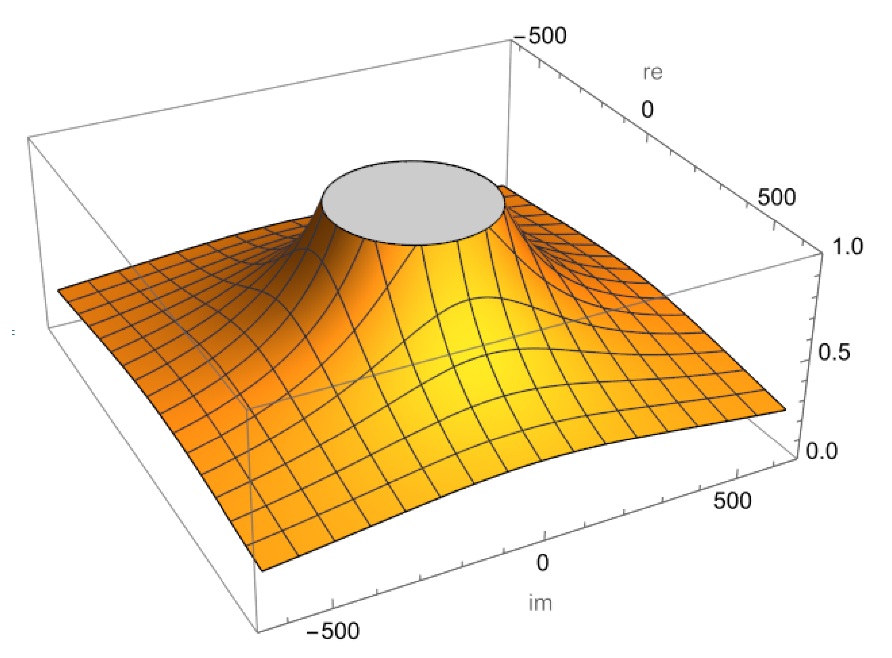
Figure 2.
Behavior of fixed points in attraction zones.
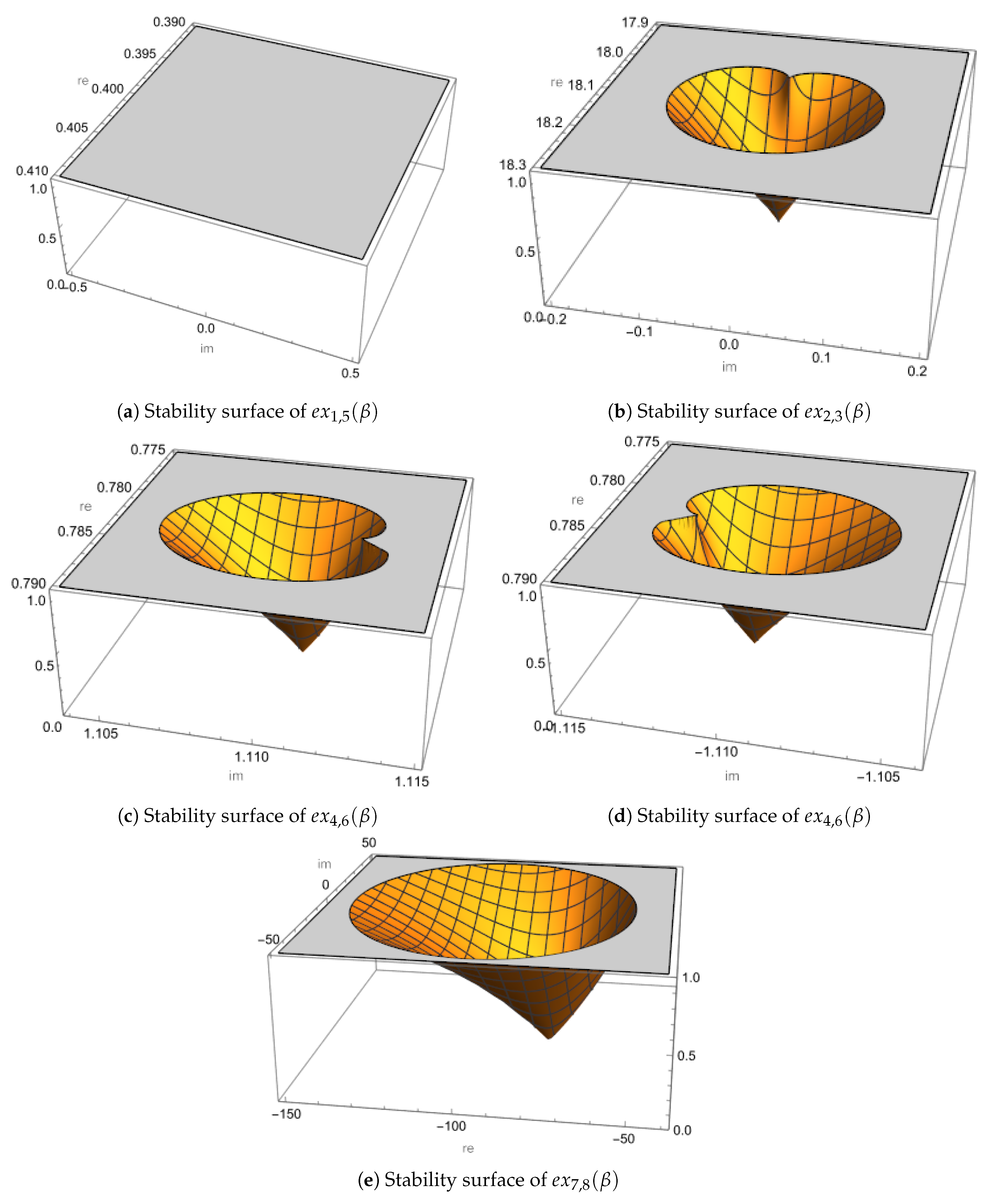
Figure 3.
Plane of parameters of in domain and a detail in .
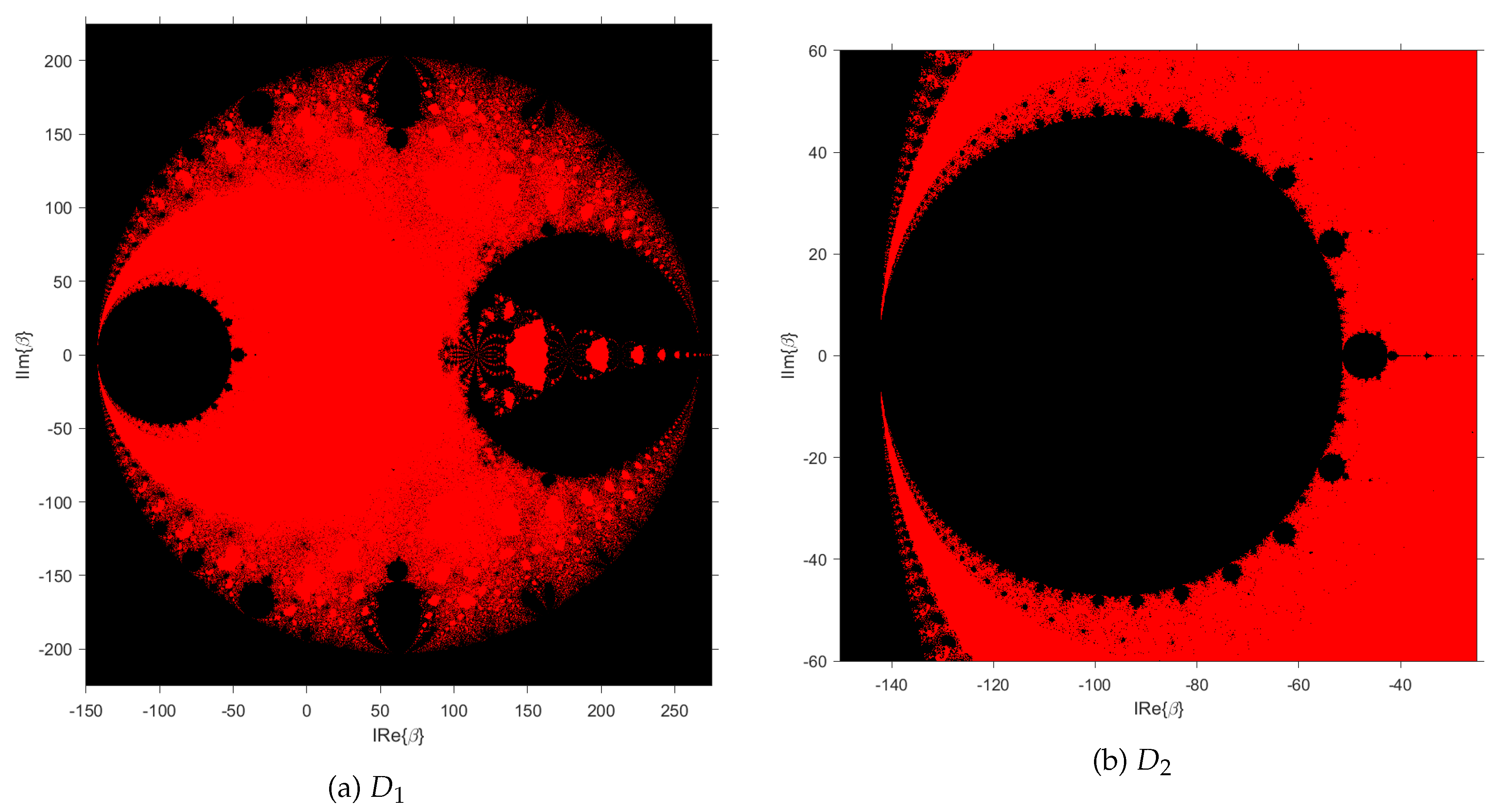
Figure 4.
Plane of parameters of in domain and a detail in .
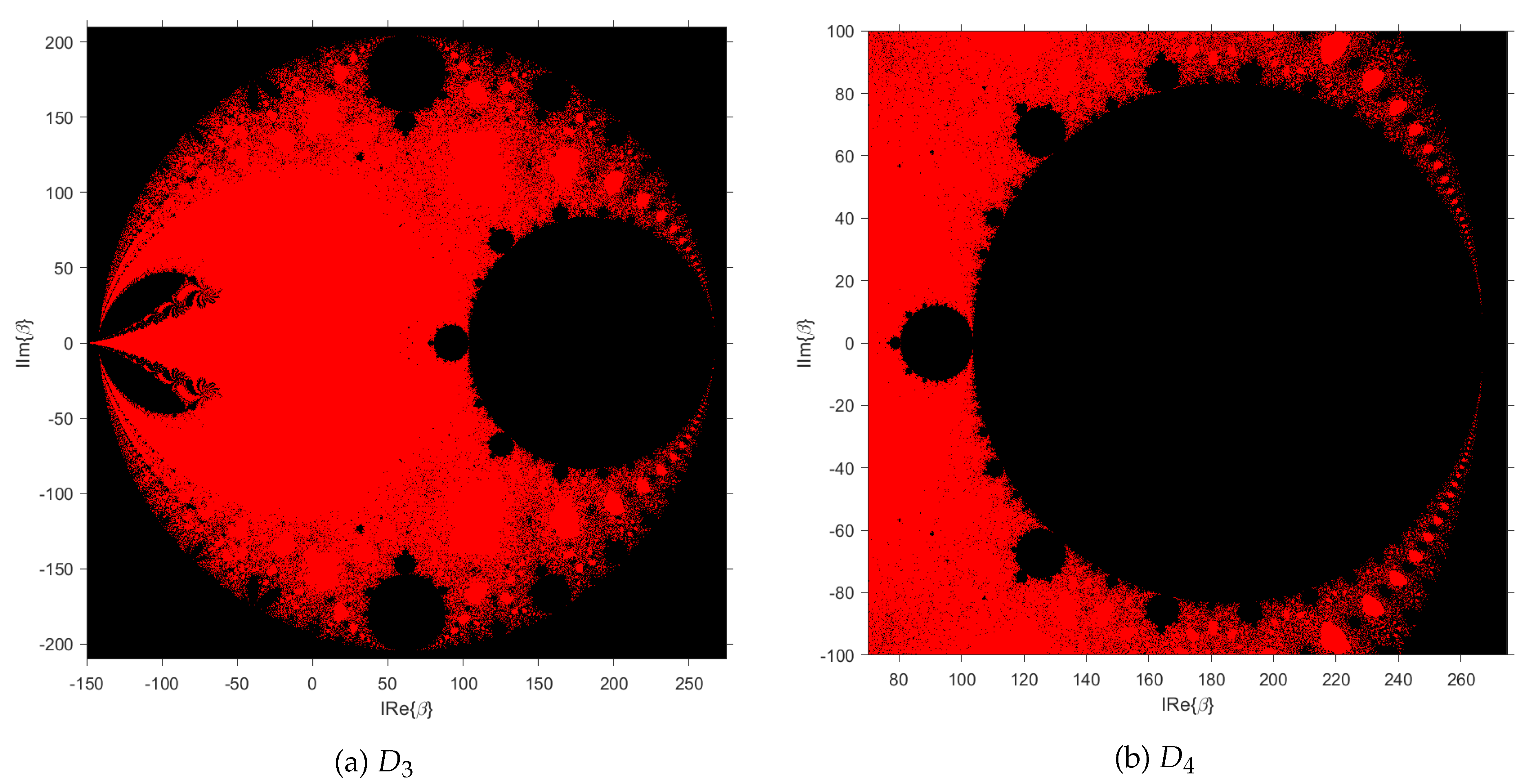
Figure 5.
.
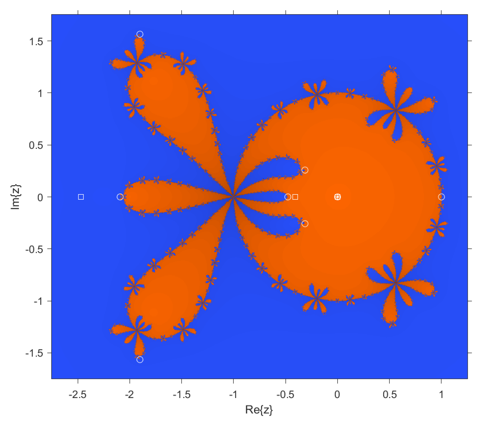
Figure 6.
.
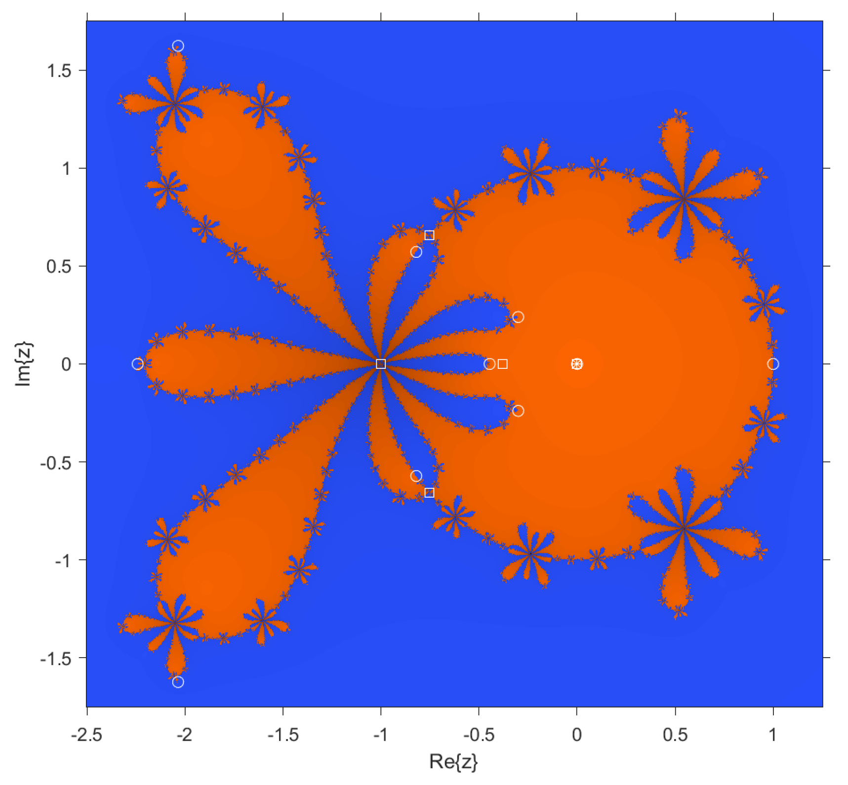
Figure 7.
.
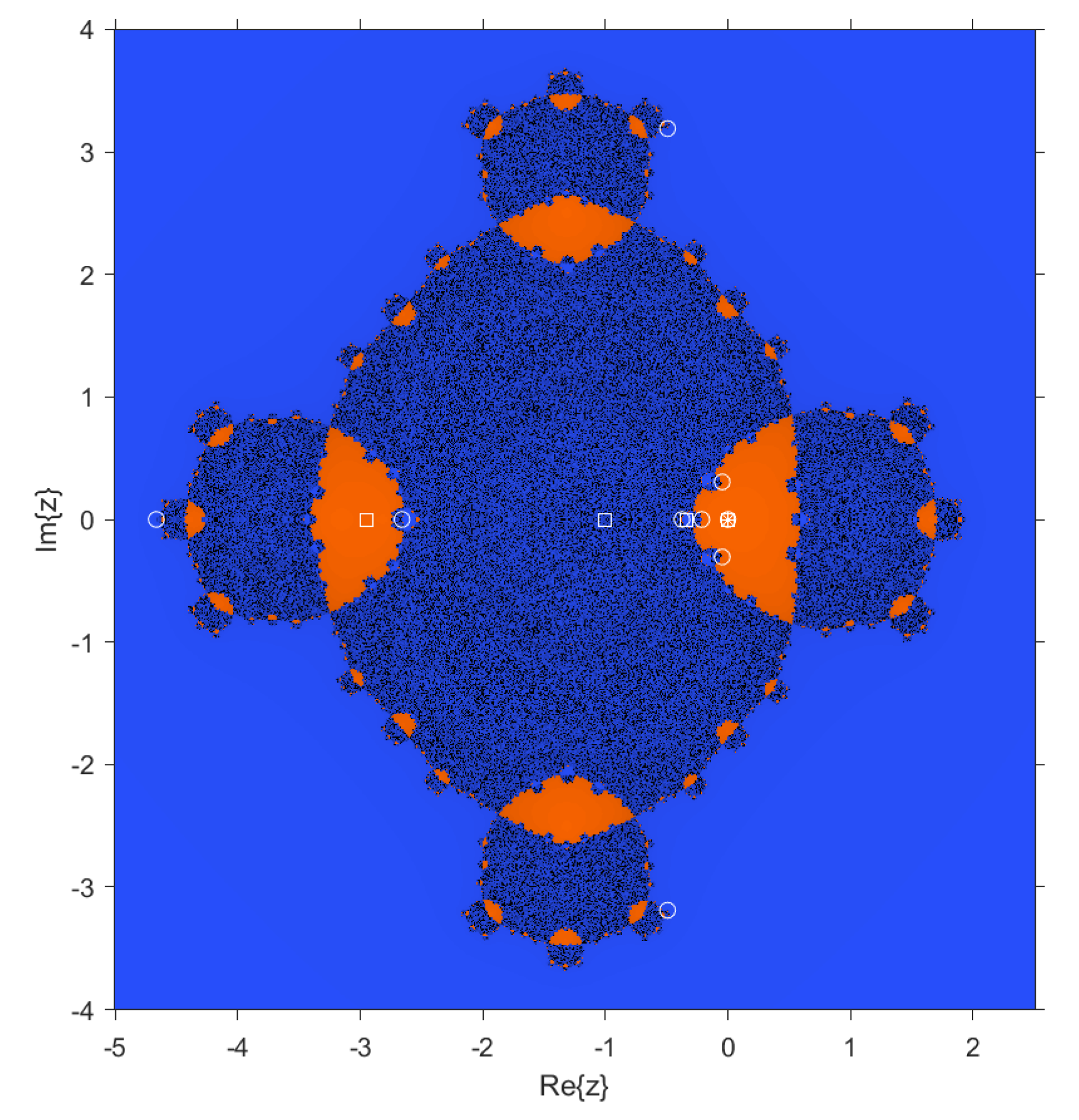
Figure 8.
Approach to .
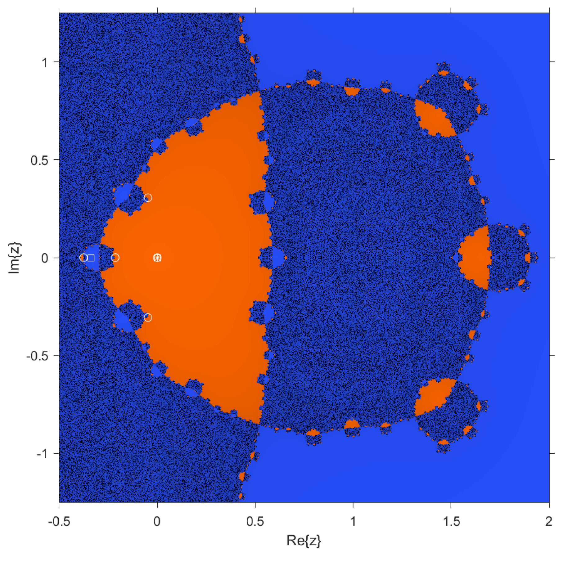
Figure 9.
.
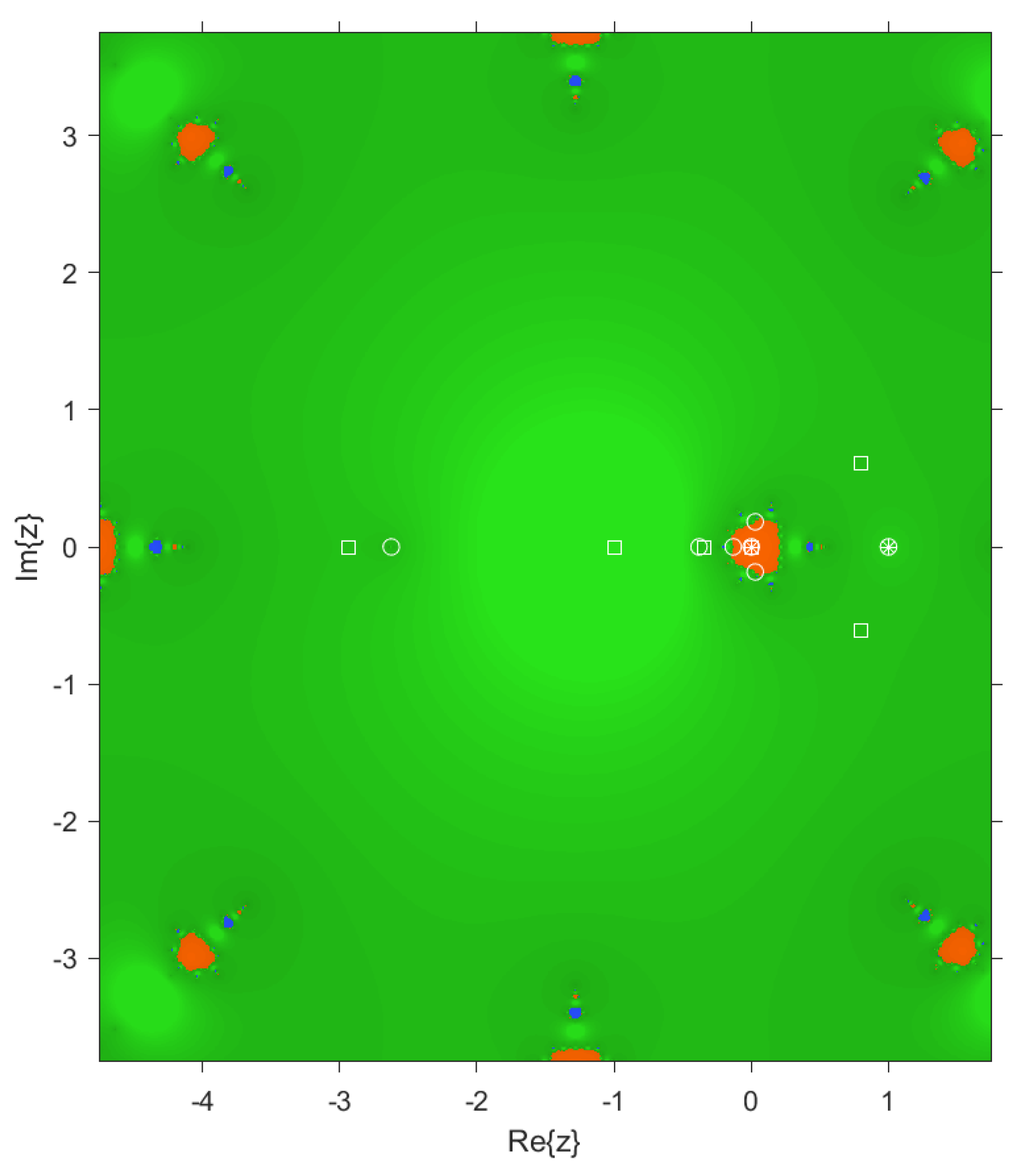
Figure 10.
Evaluation at .
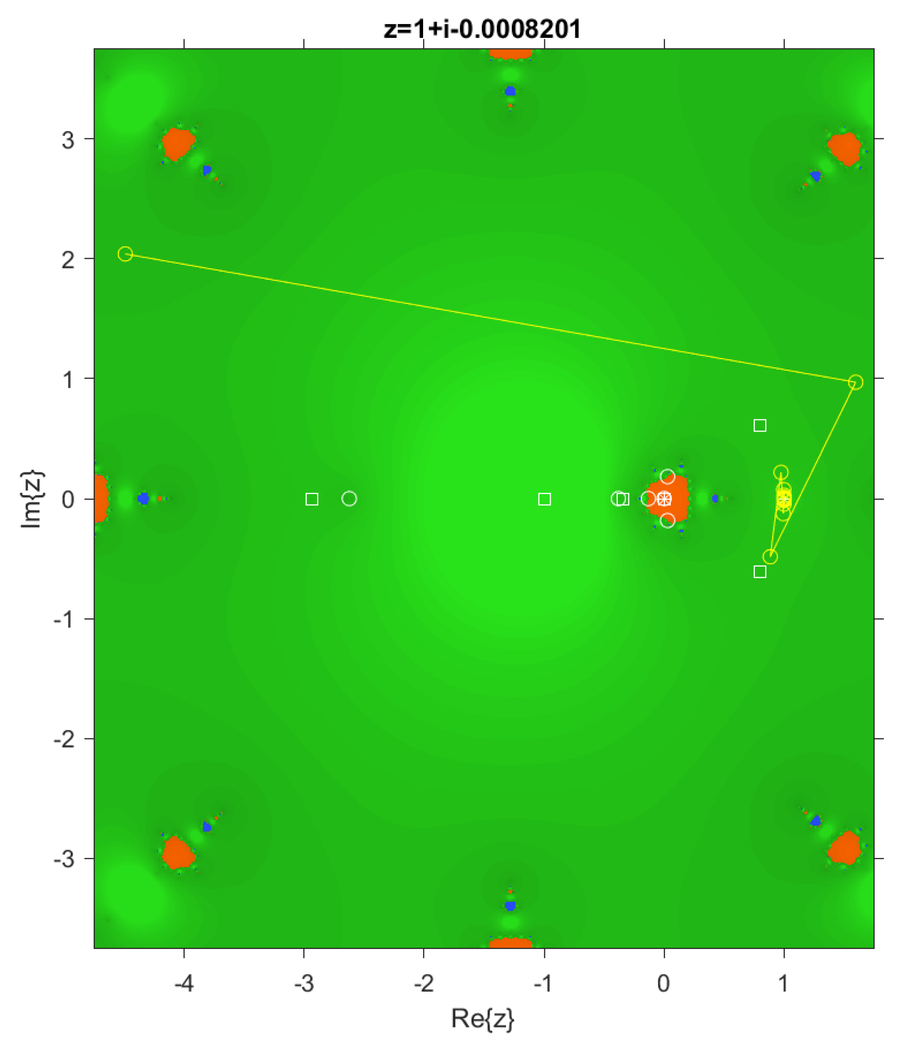
Figure 12.
.
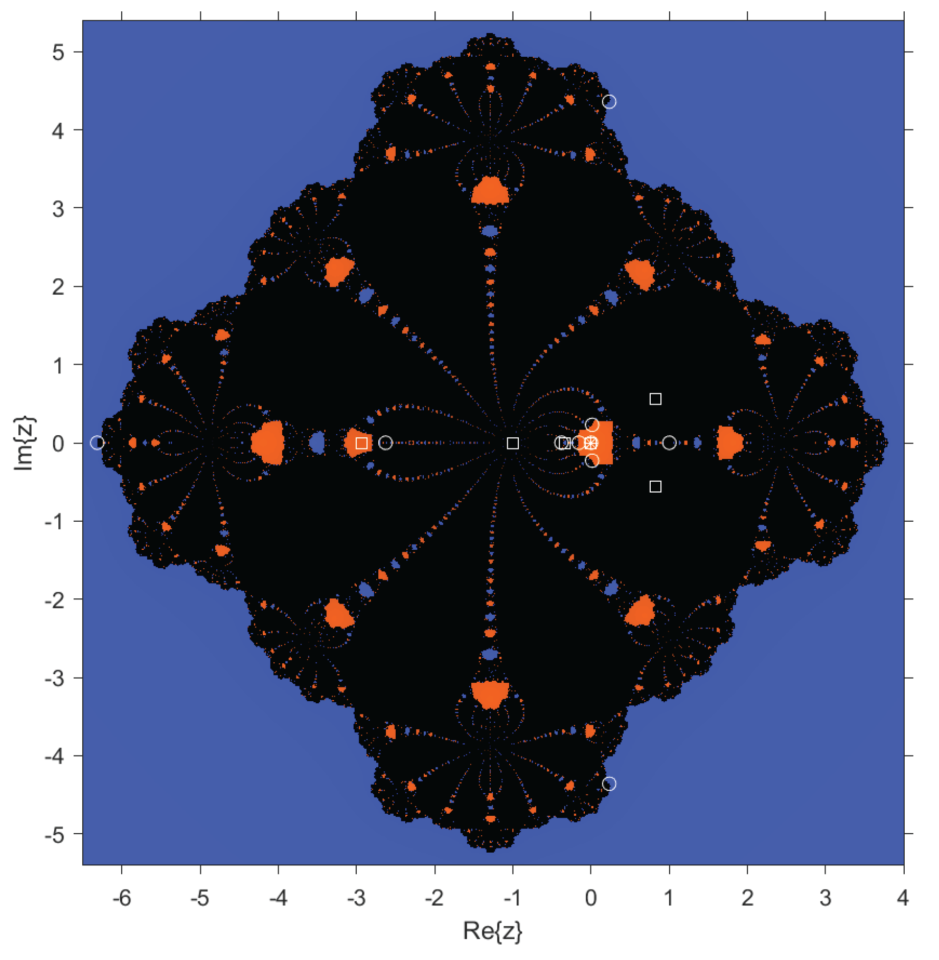
Table 1.
Summary of Fourth-Order Iterative Methods.
| Author | Iterative Method | |
|---|---|---|
| Chun (MEDCH4) [11] | ||
| Ostrowski (MEDOS4) [12] | ||
| King (MEDK4) [13] | ||
| Kung–Traub (MEDKT4) [15] | ||
| Zhao et al. (MEDZ4) [16] | ||
| Artidiello (MED44) [14] |
Table 2.
Iterative methods defined via different symmetric means , along with their abbreviations and corresponding correction steps.
Table 2.
Iterative methods defined via different symmetric means , along with their abbreviations and corresponding correction steps.
| Method | Mean | Correction Step |
|---|---|---|
| Arithmetic | ||
| Arithmetic with | ||
| Harmonic with | ||
| Contraharmonic | ||
| Contraharmonic with |
Table 3.
Coefficients of and Error Equations.
| Mean | Coefficients of | Error Equation |
|---|---|---|
Table 4.
Families of Fourth-Order Iterative Methods Based on Means.
| Mean | Iterative scheme | |
|---|---|---|
Table 5.
Performance comparison for .
| Method | Iter | Incr | Incr2 | ACOC | EI | Time (s) |
|---|---|---|---|---|---|---|
| 4 | 3.995 | 1.587 | ||||
| 5 | 4.000 | 1.587 | ||||
| 5 | 4.000 | 1.587 | ||||
| 4 | 3.840 | 1.566 | ||||
| 5 | 4.000 | 1.587 | ||||
| Jarratt | 4 | 3.998 | 1.587 | |||
| Ostrowski | 4 | 3.998 | 1.587 | |||
| King () | 4 | 3.980 | 1.585 | |||
| Kung-Traub | 5 | 3.001 | 1.442 | |||
| Zhao et al. | 5 | 3.999 | 1.587 | |||
| Chun | 4 | 3.998 | 1.587 | |||
| Artidiello IV | 5 | 4.250 | 1.620 |
Table 6.
Performance comparison for .
| Method | Iter | Incr | Incr2 | ACOC | EI | Time (s) |
|---|---|---|---|---|---|---|
| 4 | 4.000 | 1.587 | ||||
| 5 | 4.000 | 1.587 | ||||
| 4 | 3.926 | 1.578 | ||||
| 4 | 3.964 | 1.583 | ||||
| 4 | 3.924 | 1.577 | ||||
| Jarratt | 4 | 4.000 | 1.587 | |||
| Ostrowski | 4 | 4.000 | 1.587 | |||
| King () | 4 | 3.995 | 1.587 | |||
| Kung-Traub | 5 | 3.000 | 1.442 | |||
| Zhao et al. | 4 | 4.042 | 1.593 | |||
| Chun | 4 | 4.000 | 1.587 | |||
| Artidiello IV | 4 | 4.109 | 1.602 |
Table 7.
Comparison of iterative methods for the chemical equilibrium problem.
| Method | Iter | Incr | Incr2 | ACOC | EI | Time (s) |
|---|---|---|---|---|---|---|
| 4 | 3.996 | 1.587 | 0.1490 | |||
| 5 | 4.000 | 1.587 | 0.1331 | |||
| 4 | 3.995 | 1.587 | 0.1218 | |||
| 4 | 3.995 | 1.587 | 0.1058 | |||
| 4 | 3.995 | 1.587 | 0.0974 | |||
| Jarratt | 4 | 3.996 | 1.587 | 0.1188 | ||
| Ostrowski | 4 | 3.997 | 1.587 | 0.0617 | ||
| King () | 4 | 3.996 | 1.587 | 0.0630 | ||
| Kung-Traub | 4 | 2.994 | 1.441 | 0.1018 | ||
| Zhao et al. | 4 | 4.001 | 1.588 | 0.0720 | ||
| Chun | 4 | 3.995 | 1.587 | 0.0492 | ||
| Artidiello IV | 4 | 3.971 | 1.584 | 0.0729 |
Table 9.
Comparison of iterative methods for the Planck problem
| Method | Root | Iter | Incr | Incr2 | ACOC | EI |
|---|---|---|---|---|---|---|
| 4.965 | 4 | 2.008 | 1.262 | |||
| 4.965 | 5 | 4.0 | 1.587 | |||
| 4.965 | 4 | 2.671 | 1.388 | |||
| 4.965 | 4 | 1.981 | 1.256 | |||
| 4.965 | 4 | 1.915 | 1.242 | |||
| Jarratt | 5 | 4.0 | 1.587 | |||
| Ostrowski | 4 | 3.942 | 1.580 | |||
| King () | 15 | 3.997 | 1.587 | |||
| Kung-Traub | 7 | 3.000 | 1.442 | |||
| Zhao et al. | 7 | 3.984 | 1.585 | |||
| Chun | 100 | 5.121 | 1.724 | |||
| Artidiero IV | 6 | 3.976 | 1.584 |
Table 10.
Comparison of iterative methods for the Planck problem with .
| Method | Iter | Incr | Incr2 | ACOC | EI | Time (s) |
|---|---|---|---|---|---|---|
| 3 | 3.466 | 1.513 | 0.0380 | |||
| 4 | 4.0 | 1.587 | 0.0638 | |||
| 3 | 3.447 | 1.511 | 0.0323 | |||
| 3 | 3.456 | 1.512 | 0.0394 | |||
| 3 | 3.452 | 1.511 | 0.0388 | |||
| Jarratt | 3 | 3.539 | 1.524 | 0.0509 | ||
| Ostrowski | 3 | 3.477 | 1.515 | 0.0323 | ||
| King () | 3 | 3.466 | 1.513 | 0.0305 | ||
| Kung-Traub | 4 | 3.0 | 1.442 | 0.0576 | ||
| Zhao et al. | 3 | 3.483 | 1.516 | 0.0411 | ||
| Chun | 3 | 3.477 | 1.515 | 0.0388 | ||
| Artidiello IV | 3 | 3.489 | 1.517 | 0.03368 |
Disclaimer/Publisher’s Note: The statements, opinions and data contained in all publications are solely those of the individual author(s) and contributor(s) and not of MDPI and/or the editor(s). MDPI and/or the editor(s) disclaim responsibility for any injury to people or property resulting from any ideas, methods, instructions or products referred to in the content. |
© 2025 by the authors. Licensee MDPI, Basel, Switzerland. This article is an open access article distributed under the terms and conditions of the Creative Commons Attribution (CC BY) license (http://creativecommons.org/licenses/by/4.0/).
Copyright: This open access article is published under a Creative Commons CC BY 4.0 license, which permit the free download, distribution, and reuse, provided that the author and preprint are cited in any reuse.