
Submitted:
04 September 2025
Posted:
05 September 2025
You are already at the latest version
Abstract
Coordination algorithms are required to minimise congestion when every robot in a robotic swarm has a common target area to visit. Some of these algorithms use artificial potential fields to enable path planning to become distributed and local. An efficiency measure for comparing them is the time to complete a task in relation to the number of individuals in the swarm. To compare distinct solutions as the swarm grows, experiments with different numbers of robots must be simulated to form a plot of the function of the task completion time versus the number of robots or other parameters. Nevertheless, plotting it for many robots through simulation is time-consuming. Additionally, the inference of a global swarm behaviour as the task completion time from the local individual robot motion controller based on potential fields and other dynamical variables is intractable and requires experimental analysis. Based on that, equations are presented and compared with simulation data for estimating the expected task completion time of state-of-the-art algorithms, robots using only attractive and repulsive force fields and mixed teams for the common target area problem in robotic swarms with not only the number of robots as input but also environment- and algorithm-related global variables, such as the size of the common target area and the working area, average speed and average distance between the robots. This paper is a fundamental first step to start a discussion on how better approximations can be achieved and which mathematical theories about local-to-global analysis are better suited to this problem.
Keywords:
robotic swarm
; common target
; time estimation
; local-to-global analysis
1. Introduction
1.1. Motivation
Robotic swarms are systems formed by often simple robots with distributed processing and local sensing [1]. As it happens in insect swarms, no centralised coordination is performed for controlling each individual. Thus, distributed control and local sensing are assumed in robotic swarms [2,3].
As a way to reduce costs, robotic swarms use many simple and cheap robots instead of relying on a few complex and expensive ones [4]. Creating complex group behaviours based on simple rules is the goal of some robotic swarm research [1,5]. Counter-intuitively, such complex global behaviours may emerge from well-planned local rules. [6,7]. Consequently, swarm designers have to infer from local rules a global result needed to solve their problems. This inference may arise from several simulations of the local rules. However, when dealing with many robots, simulations could be time-consuming, and estimations of the resulting global outcome would be useful for swarm designers.
Having that in mind, this paper focuses on estimating a global outcome, the completion time of a task performed by some number of robots in a swarm, based on the robot’s local specification in a problem that may occur when numerous robots of that swarm have the same area: the common target problem [8]. This problem may occur, for instance, when robots are deployed to collect a leaked toxic substance. These robots need to coordinate themselves to reach that region as fast as possible while not interfering with the collection of the other robots. If the robots do not execute an efficient traffic control algorithm, their mutual interference can worsen.
Hence, solutions to the common target problem can also be applied in waste collection [9,10] in secluded areas such as the ocean, disaster response [11], construction [12], searching of cancer cells by microscopic robots [13,14,15,16], rescue in regions harmful to humans [17] and warehouse management [18,19]. In this problem, the number of robots inevitably may cause congestion as they are forced to share the same area. In addition, this number can impact the execution time, which affects other measures (e.g. heat generation and energy consumption [20]).
Thus, when devising different solutions for this problem, the typical practice is to compare the task completion time with the number of robots and environmental or algorithmic parameters (e.g., working area and target area sizes) [8,21,22,23]. For the common target problem, artificial potential fields are usually applied to such solutions in the same manner as in robotic swarms due to their distributed and local characteristic for path planning [24,25,26]. Additionally, other collision methods may not work well for this problem. For instance, Marcolino et al. [8] performed tests with the distributed collision avoidance method ORCA, which does not work for the common target problem because the robots enter a circular deadlock, not reaching the target area. The recent GBP Planning [27] requires the additional cost of using communication between robots, while the algorithms mentioned in this work do not need it.
That being said, when the local individual specification based on potential fields is modified, global swarm behaviours, such as the task completion time, will have specific outcomes accordingly. To compare distinct potential fields that work better for various numbers of robots, experiments with different values must be simulated to form a plot of the function of the task completion time versus the number of robots or other parameters. Nevertheless, plotting it for many robots through simulation is time-consuming. A swarm designer could use estimations instead of simulations to choose between available solutions.
An alternative approach would be using regression over the experimental data. However, it does not explain the time in relation to the number of robots, dynamical variables such as average speed, the average distance between the robots, and environmental or algorithmic variables such as the radius of the target area, radius of the task working area and how many directions the robots must go after they reach the target area.
Additionally, there are many situations where different swarm teams may be present in the same environment. For instance, such mixed teams (MT) can be found in the multi-agent literature [28] in problems like Pursuit-Evasion Games [29,30] and Multi-Agent Pickup and Delivery [31]. This work considers mixed teams where each group does not know the algorithm used by the other groups. This could happen, for example, in a situation where a robotic swarm runs some coordination algorithm for accessing an area for rescuing people in an accident, and different institutions want to help. Assume that they deployed their robots and, for a fast response, did not meet to settle the swarm congestion control algorithm for quickly accessing the common area. Then, the first swarm to arrive will execute a congestion control algorithm, but the next does not know which algorithm is in execution.
This is an example of ad hoc teamwork [32] and usually agents use learning about other agents to handle it [33,34,35]. However, the above situation requires a fast response, but learning needs long iterations of training, and errors may be introduced during the learning process. Thus, it is considered here that each group of robots in MT executes a fixed algorithm without spending time on learning the algorithm of others. If these algorithms happen to be the same across all groups there will be no impact in the swarm by mixing them. However, if they are different, they may affect each other negatively. Therefore, the influence of different algorithms is also analysed here. In fact, this work shows that the expected task completion time estimations are also applicable to estimate the expected task completion time of mixed teams.
1.2. Objective
The objective of this paper is to introduce estimations of the expected task completion time according to the number of robots and environmental and algorithmic parameters in algorithms for the common target problem using potential fields. As these estimations are difficult to be expressed directly from the individual robot controller, they are based on analysing the observations made by simulating the control swarm algorithm. The equations of these estimations are mainly derived from geometric characteristics of the usual behaviour of the robots by following the control algorithm or obtained from well-known equations cited in the explanation of the estimation. No paper has presented such estimations for that problem before. Thus, this paper is a fundamental step to initiate a discussion about how the global system behaviour can be inferred from individual potential field-based local controllers in Swarm Robotics.
For doing so, extensive experiments were performed in the realistic Stage simulator [36] due to its easiness of running in batch and parallel, low memory cost, fast execution for numerous robots and recent usage and review [37,38,39], assessing the completion time from hundreds of robots as quick as possible to generate graphs and analyse different parameters. The proposed estimations are compared with data from experiments for a swarm with no coordination [21], state-of-the-art algorithms Single Queue Former and Touch and Run Vector Fields [23] and two groups in MT. Also, these algorithms are modelled in equation form to highlight the difficulty of directly deducing the task completion time from them. Experiments with them were made from 20 to 300 robots and different circular target area radii with holonomic and non-holonomic robots, to show the adaptability of the estimations to divergent types of robot movement. For MT, all combinations of those algorithms were tested to show the suitability of each algorithm for different ratios of the number of robots in a group to the total number of robots. The root mean squared error normalised by the y-axis range (NRMSE) values of the estimations are between 0.011 and 0.028 for a swarm without different groups and between 0.008 and 0.036 for two groups in MT.
1.3. Paper Organisation
This paper is organised as follows. The next section discusses the related work, including studies of local-to-global in science, the many-body problem and its application in Swarm Robotics and the robotic swarm common target problem and the algorithms to solve it.
Section 3 presents the task completion time estimations and how they were obtained for a swarm using only attractive and repulsive force fields, state-of-the-art algorithms and Mixed Teams. In that section, each algorithm is stated in its equation form and exemplified with key screenshots of some executions. These examples are samples of the observations used for describing how these estimations are approximated. Thus, following each estimation, an explanation shows the derivations of these approximations developed from those observations made by simulating the algorithm.
Section 4 describes the experiments performed to corroborate the estimations derived in this work and discusses their results. These experiments aim to compare the estimations with the data obtained from simulations.
Section 5 discusses the limitations, challenges, improvements over this work and how the methodology can be applied to similar problems in Swarm Robotics.
Finally, Section 6 summarises the results and concludes this work.
2. Related Work
The effect of the task completion time of a robotic swarm based on the dynamic of one individual is an example of an analysis from local to global. Similar works can be found in other study areas. In special, the many-body problem in Physics has elegant and strong mathematical solutions. Some works for traffic problems or Swarm Robotics have applied solutions for the many-body problem. However, the solutions presented are not adequate for the common target problem. The algorithms developed for the common target problem mostly use potential fields as a local path planner to emerge global congestion control. These works will now be discussed in detail.
Studies of Local-to-Global: Biology, Chemistry and Physics share the study of individual parts of different systems to explain their global behaviour. The manifestation of emergence [40,41,42,43] is a good example of such studies. In it, the microscopic characteristics enable the arising of unexpected macroscopical behaviour. As the understanding of these relations grows, advances in other areas like engineering and robotics are made. Related to that, the interdisciplinary Synergetics [44] explain self-organised phenomena in systems with non-equilibrium such as cloud dissipation, lasers and patterns in slime mould or chemical reactions.
The Many-Body Problem and Solutions: In Physics, problems about the interaction of microscopic particles is generally mentioned as the many-body problem [45,46]. For instance, in statistical mechanics, the Maxwell-Boltzmann distribution function [47,48] states the speed probability distribution of ideal gas particles. It is calculated by analysing the movement of the particles under the influence of gravity and the probability frequency of the energy from the distance to the ground. Then, the velocities are averaged over all directions and that probability frequency to yield the desired distribution. There are different approaches to this problem. The perturbation theory [49,50] starts with a simpler version of the problem. Then, an expression, often called perturbative expansion, using power series of successive corrections to the simpler problem is developed to solve the original problem. The coupled cluster technique is used in computational chemistry [51,52] for solving this problem numerically. Similarly, the density-functional theory [53,54] is applied in computational modelling to understand the electronic and molecular organisation from atoms to solids by using functionals of electron density that depend on the space. The mean-field theory [55] substitutes the high number of interactions between the particles with a few averaged ones, reducing the number of calculations but also the exactness of the solution. There are interesting applications of this method in multi-agent research such as Chen et al. [56], Lasry and Lions [57]. The variational method [58,59] is a solution similar to that used in quantum mechanics for approximating the desired energy state by selecting wave functions whose parameters minimise the expected value of the energy. The neural network quantum states [60] approximate the solution using machine learning to minimise the variational energy.
Similar to Many-Body in Swarm Robotics: Additionally, the literature on many-body problem is mostly Physics-oriented. An interesting approach to the intersection of Physics and Swarm Robotics is described by Hamann [61], where he applied Brownian motion, Langevin equation and Fokker-Plank equation for estimating global behaviour from individual robot specification by random movement. Another approach to the above solutions for the many-body oriented to real-world application is the Herman-Prigogine kinetic equations for vehicular traffic [62,63,64], considering the drivers with intentions but random actions. However, as these approaches give results assuming that every action of every driver or particle is random as time passes, their equations cannot be applied directly in this work because only the initial position is random, but all the movement is deterministic. The survey of Elamvazhuthi and Berman [65] also presents another study on Swarm Robotics and Physics aligned with the problem in this paper, but the references provided by Elamvazhuthi and Berman [65] do not directly answer the research question shown here. Instead of assuming randomness in the movement of the individual robots and showing purely theoretical deductions, the estimations calculated here use experimental observation from simulations performed in Stage [36]. Additionally, these estimations are a fundamental first step to start a discussion on theoretical aspects on the relation of time and the number of robots on the common target problem.
The Robotic Swarm Common Target Area Problem and Algorithms: The common target problem is usually handled by using potential fields [8,21,23]. In fact, the algorithms discussed in Section 3 use them in the role of an individual path planner to accomplish global congestion control. Any of these algorithms modify the attractive and the repulsive force field to minimise the time to access the common target area or the task completion time, which, in addition to the time to access it, includes the time for leaving it. This may bring to light the question about whether it is possible to find the exact attractive potential field that minimises this time by a method similar to the Lagrangian in mechanics [66], which elegantly solves curves with minimum energy requirement using stationary action or with variability as in the many-body approaches discussed above. For finding such a minimal potential field, the function of the task completion time per number of robots has to be obtained beforehand. As far as the authors know, no work presents how to obtain this function from the motion equations of a robot, which is a challenge in Swarm Robotics. Thus, experimental approximations are presented in this paper by observing the swarm, making this work a fundamental first step for studying the common target problem as a local-to-global analysis to serve as a basis for comparing new approaches for a theory capable of finding such minimal potential field.
3. Expected Task Completion Time Estimation Analysis
In this section, the estimation analysis is presented by describing the task scenario of the experiments, the individual robot controller, the challenge in the development of a global analysis from local controllers and the common settings of the algorithms for which the expected task completion time estimations are analysed for a number of robots in the swarm.
Task Scenario: Consider the task scenario where a system with N robots in a plane must reach a common target located at . Each robot knows its position and the positions of the targets, and it can sense nearby objects (for instance, by using laser scanners covering 360 degrees). Upon reaching the target, the robots move to different destinations, which may not be similar. Suppose that the target area is a circle of radius s, and a robot reaches the target if its centre of mass is at a distance below or equal to the radius s from the centre of the target. In addition, there is no minimum amount of time to stay at the target.
In this scenario, the coordination algorithms, if applied, are only employed inside a working area, that is, a circle of radius around the target. Although the swarm density is not considered as an explicit parameter in this work, the number of robots N and the radius D of the working area yield the swarm density . If the robots have two or more targets, the targets are apart by at least . The initial position of the robots has a distance from the target centre randomly chosen from a uniform distribution in m for a fixed E. The angle between the initial position of a robot and the x-axis is selected from a uniform distribution in rad. To avoid robots starting in the same position and crashes between robots in the beginning of the simulation, if the distance between a robot and any other is less than 1 m, its initial position is selected again. This arrangement inside an annulus is only considered at the start of an experiment and before the initial target.
Once the robots have reached the first target area, they will proceed to the next one at a long distance, either to the left or right of the shared target. In other words, the next target is chosen randomly between positions and . Thus, approximately half of the robots will go to the left-hand side and the rest to the right, according to a uniform probability. This paper focuses on the congestion around the first target area, which is shared by all the robots in the swarm. After they leave the working area around the shared target area, they head towards the next target area by using only repulsive and attractive forces (that is, they turn off the coordination algorithm). In addition, the robots measure in the experiments. Although some settings are precise (e.g., robot size and next target positions), the equations derived in this paper are based on general behaviours and are applicable with different parameters.
The global metric analysed in this paper from the local individual robot controller is defined below.
Definition 1.
The task completion time is obtained from the last robot to leave the working area around the shared target area, that is, the maximum time to enter the shared target area plus the time to leave the working area for every robot in the swarm.
Once a robot leaves the working area after it reached the first target area, it is no longer considered in the computation of any metric presented in this paper. As the initial position of the robots is random in an experiment and influences the variation of the task completion time, it is considered the expected task completion time from various experiments, which is defined below.
Definition 2.
Let be the task completion time of an algorithm using N robots for an experiment with the initial position of the N robots fixed. Then, stands for the expected task completion time over all executions for N robots.
Individual Robot Controller: Consider a robot at position at time t. In this work, each robot uses the same movement controller, chosen to physically describe the change in the position of the robot given by any algorithm that has an input force resultant from a potential force field , for an attractive potential field and a repulsive potential field . The input force has to be equal among the robots for all algorithms to perform a fair comparison among different approaches. Also, the controller needs to adapt the acceleration when the robot’s velocity changes in situations such as the sudden advent of another robot or the transition to a new target. To satisfy these requirements, the controller is based on the previous works on the common target problem [8,21,23] but rewritten in continuous form: , and
where is a force to attract the robot toward a target, and is the repulsive force applied to avoid bumping other robots. Without the assumption that the robot knows the target position, cannot be computed correctly. depends on the algorithm used by each robot and has a fixed magnitude . The sections below show different choices for . Each robot adds the attractive force with the repulsive forces and then constrain the result to a fixed vector modulus to homogenise the acceleration among the individuals in the swarm. The constant is employed to control alterations in velocity. It prevents the robots slipping due to acceleration changes.
Also, the following repulsive force is employed because it acts as a strong barrier as the robot approaches an obstacle [67]:
where is a fixed multiplicative constant for the repulsive force field, and is the default influence radius, that is, the maximum distance from its mass centre a robot considers anything sensed as an obstacle to avoid. can be set to the maximum range of the robot’s local sensor. Thus, a robot deprived of local object sensing cannot compute .
Challenge in the Development of a Global Analysis from Local Controllers: With that , Equation 1 depends on the neighbourhood of the robot, which, although limited, is dynamic. Even if there is a fixed maximum number of neighbours, a global analysis of would depend on all the other robots for each instant t. Thus, obtaining a closed-form expression for the task completion time in terms of N directly from Equation 1 is difficult. In addition, observing the behaviour of an algorithm for hundreds of robots in the real world is expensive, but it is faster and more affordable by simulation.
In other words, if the individual robot control equations were simpler than Equation 1, the closed-form expression of the expected task completion time in terms of N would be obtained by the following steps: (i) integrate Equation 1 twice to obtain for , (ii) invert it to retrieve t for each robot i, (iii) obtain the maximum t for every robot i and (iv) calculate the expected value of this maximum when the initial positions of the robots are randomly distributed inside the annulus of radii D and and centre at . As this closed-form expression cannot be derived from Equation 1 in such manner, a theoretical macroscopic analysis inspired by simulations is performed to attain an approximation of the expected task completion time . For doing this, besides the target area radius s and the working radius D, the following variables are given: the mean distance between the centre of mass of a robot and the others inside the influence radius for all robots and the mean linear speed of all robots . A summary of the variables most used henceforward is in Table 1.
Moreover, the approximations stated in this section may use these variables as input and are mainly derived from geometric observations or obtained from well-known equations. These approximations are explained after their statements, based on a macroscopic analysis observed from the simulations. As these approximations are constructed from experimentation, these explanations cannot be considered formal proofs, although they are composed of proven mathematical expressions.
Furthermore, in the expected task completion time expressions shown below, constants are defined for each algorithm to subsume the overall behaviour of the robots, their interactions and the congestion inspired by the experiments. Such abstraction is analogous to the friction constant in Physics, which summarises the microscopical effect of surfaces. In this field of study, the friction constant for commonly used materials was initially calculated from experiments with them. Similarly, the defined constants are fitted by the experimental data in Section 4.
Common Settings of the Presented Algorithms: In this section, four algorithms are analysed about the expected task completion time. In the examples in the figures that follow and in the performed experiments, it was used the values in Table 2 and the robots are holonomic. Note, however, that the theoretical results also apply for arbitrary values and holonomic or non-holonomic robots, as shown in Section 4.
In the following sections, the state-of-the-art algorithms in [23] are restated in equation form and based on the local motion controllers for showing the difficulty of solving the task completion time from the individual local control equations. This presentation begins with the no coordination (NC) [21] (that is, without any congestion control algorithm, only attractive potential field to the target area and repulsive potential field for avoiding other robots) as a simple example to show that, even from this reduced model, it is hard to infer the expected task completion time per number of robots.
3.1. No Coordination Algorithm
Algorithm Description: When the robots are not coordinated, they only follow the target region, avoiding the others by repulsive force. The equation for the in Equation 1 is the attractive force to the target centre given by
Although this is the simplest attractive force of all algorithms presented here, Equation 1 also considers the repulsive force of all robots in the environment. Thus, as the number of robots grows, the analytical solution for the differential equations is still complicated to infer.
Samples of the Observations: As an illustration, Figure 1 and Figure 2 show an experiment of NC. Red robots are going to the target region, yellow ones have arrived at it and are trying to leave it, and black robots have exited from the working area and are going to the next target. The robots start in random positions outside the working area (Figure 1(a)). The first robot to reach the working area takes an expected time inversely proportional to the number of individuals in the swarm (marked with a circle and an arrow in Figure 1(b)). Each robot goes toward the target area until the first reaches it . Eventually, the first robots to reach the common target area will be stuck in it and will try to leave while they are slowed down due to the congestion caused by the other robots that did not arrive at the target yet (Figure 1(c)). The robots trying to leave the target area will slowly push the other robots until they move out of the cluttered region with a shape similar to a circle. If a robot is heading in the same direction as the first to overcome this area, it may follow the space created by the other robots avoiding the first. This may cause more robots to do the same, and a queue of robots is formed (Figure 1(d)). The length of this queue and the number of robots in it are random. New queues may appear while the number of robots in the cluttered area diminishes. When no robots are trying to arrive at the target area, the last queues of robots will finally reach the outside of the working area (Figure 2(e)) until the last robot leaves this area (with a circle and an arrow in Figure 2(f)).
Figure 3 and Figure 4 illustrate an example with a larger target area radius. The robots have more space to access the target. In this example, the capacity of the target area is greater than the number of robots, so they can use the free space to travel to the next targets in both sides (Figure 3(c)). Due to this free space, the number of robots going to the target (in red) is not enough to force the robots leaving it (in yellow) to go to the target centre (Figure 3(d)). Thus, the time until the cluttering near the target area disappears is lower than in the previous example, and how the robots leave the target area is also different (Figure 4(e)) because of the free space in the target area and the less resistance caused by the robots going to the target area.
By analysing such examples, an approximation of the expected task completion time for the NC algorithm can be obtained. The following estimation presents the result. After its statement, an explanation shows the derivations of that approximation based on the observations made by simulating the algorithm. Because the following estimation is constructed from experimentation, the explanation below cannot be considered a formal proof.
Estimation 3.
The estimated expected time for N robots starting at a random position with a distance from the target centre in to arrive at the common target area and leave the working area without coordination is
for
and constants and .
Explanation.
The equation for estimating the expected time for NC has five parts: the expected time for (a) the first robot arriving at the working area from its starting position, (b) the first robot that entered the working area reaching the target area (e.g., the time at Figure 1(b)), (c) the first robots filling the target area (e.g., the time from Figure 1(b) to 1(c)), (d) the cluttered area disappearing by the queues of robots leaving the target (e.g., the time of Figures 1(c)–2(e) and 3(c)-4(e)) and (e) the last robot that reached the target leaving the working area (e.g., the time from Figure 2(e) to 2(f)).
Part (a) is obtained from the expected value of the minimum starting distance to the working area for the N robots. Due to the task scenario description, this value uniformly ranges in . Consequently, the expected minimum distance is , obtained from the probability distribution function of the minimum value [68, p. 229]. Then, the expected time for the first robot to arrive at the working area is .
Parts (b) and (e) share the same expression, obtained from the expected time for a robot on average speed going from the end of the working area to the target area and vice-versa: . Part (c) is given by the expected time for a robot going from the border of the target area to the target centre due to the congestion caused by the other robots going to the target area: .
For calculating the time (d), there are two cases. Let the capacity of the target area be the maximum number of robots that fit inside the target area. When the capacity of the target area is greater than or equal to the number of robots outside the target area, the robots which arrive at the target area have less resistance to leave through the space between the robots which did not yet. The capacity of the target area is approximately the number of circles of radius – half the mean distance between the robots – inside the target area with radius s increased by , that is, . Thus, the number of robots exceeding the capacity of the target area is less than or equal to its capacity if . From experiments, the waiting time can be approximated by for a constant that abstracts the influence of other factors in this time, assuming that it does not depend on time (e.g., any scaling in the speed or the average number of robots per queue, and the influence in the overall movement by the type of the robot – holonomic or non-holonomic).
If the maximum number of robots that fit inside the target area is less than the number of robots outside the target area, the resistance for leaving the target area is higher than before, and part (d) is calculated differently. Due to the erratic formation of the queues of the robots leaving the target area, the time is approximated by assuming a fixed mean distance between the robots and mean speed moving from the cluttered area and taking the same time to move as the erratic queues. As seen in the example from Figure 5, the robots outside the target area go towards the centre, while those leaving it form queues following the other robots for each direction to overcome the congestion. The red robots going to the target tend to concentrate inside a circle containing the cluttered area. On the other hand, the yellow robots leave that area one by one for each queue, diminishing the number of robots in the clutter.
Hence, the cluttered area is approximated by a circle whose radius vanishes as the robots run through these queues. Let be the number of robots in that circle at time t. Figure 5 illustrates this circle with robots. The cross mark in the middle indicates the target area centre. Suppose that a robot next to that position has to leave that circle. Then, it must run a distance of at most .
This radius can be estimated from the area occupied by robots. For this estimation, consider each robot occupying a squared area of . The area of the circle containing the robots is approximately the area occupied by squares with area , that is,
A robot next to the target centre has to move through a distance equivalent to the number of robots fitting , excluding that one. Thus, the number of robots to move through is given by . As one robot is decreased proportionally to the number of robots that it would have to move through and the number of queues, the rate of decrease is given by
subsumes the effect of other factors in this rate, such as how the robots move and variations in the speed, similar to above. Hence,
for a constant . As for , , implying that when ,
The desired result is obtained by summing parts (a)-(e) and simplifying the final result. □
3.2. Single Queue Former Algorithm
Algorithm Description: The Single Queue Former (SQF) algorithm [23] makes one queue shaped as a rectangular corridor that goes towards the target. This corridor has a width equal to the circular target diameter, , and a length equal to the working radius, D (Figure 6). The robots are permitted to enter the target region only by this queue. Potential fields are deployed to form this queue (Figure 6(a)) and to guide the robots to the target area exit (Figure 6(b)) efficiently. The corridor starts from the current target centre . Without any loss of generality, the corridor has vertices located at , , and .
A rotational force field is applied to robots in the working area to enter the common target area through the corridor. The field rotation centre is at the target centre. The robots are submitted to an attractive force towards the target once they reach the corridor. After they arrive at the target area, another rotational force field is applied to them, whose centre is either at the leftmost point of the working area, , or at the rightmost point, , depending on the position of the next target.
To control the attractive forces, each robot has the states going to the target (), leaving the target () and going to the corridor (), which respectively means the robot is going straightly to the target region, it is leaving it, and it is going to the corridor. The starting state of the robots is since they start outside the working area. Consider the conditions named W, O and A, represented as well-formed formulas:
where is the position of the robot i at time t. In other terms, W is true when the robot is inside the working area, O, when it is outside the corridor unlimited from above and A, when it has already arrived at the target area. Note that W and O do not depend on past time as A. Thus, the states of the robot can be represented as formulas using these conditions, which are mutually exclusive:
By using these conditions, the attractive force is represented as follows. Robots outside the corridor follow a force according to Passos et al. [23]
where is a constant for setting the force magnitude. In other words, for the left-hand side of the circular working area, a clockwise rotational field is applied, and for the right-hand side, an anti-clockwise one.
However, if the robots are in the corridor, they go towards the target area following the same attractive force equation as in Equation 2, that is,
Robots exiting nearby the target are constrained by another rotational field. This field also is only applied inside the circular working area:
where is the new target location. In other terms, for a robot with a new target located on the left-hand side of the previous target centre, a clockwise rotational field is applied and, on the right-hand side, an anti-clockwise one.
Finally, in addition to the default influence radius , another constant is used by the robots when calculating repulsive forces: , with , the minimum influence radius allowed. For robots inside the corridor or exiting the target region, the influence radius is . Now consider a robot outside the corridor but on the upper half of the circular working area. Let be the distance between the robot and a vertical line in the middle of the corridor (Figure 6(b)). Its influence radius I varies in relation to and is set to only for . This range for guarantees that . For the other robots, the influence radius is . Thus, the influence radius and repulsive force are given by
Observe that plugging those attractive and repulsive forces in Equations 4–7 into the movement controller (Equation 1) yields an intricate differential equation with cases that not only depend on the position of an individual robot for attraction but also the robots in the neighbourhood due to the repulsive force and past time. Moreover, the influence radius calculated in Equation 7 also has different cases, expanding the chain of related expressions to calculate the solutions of the differential equations for each robot. Due to this complexity, the inference of the SQF algorithm task completion time function from the controller equations becomes more difficult than when the robots use NC. As a result, the estimated task completion time function equation is calculated by observing the behaviour of the robots in experiments, similarly to the previous section.
Samples of the Observations: As an example, Figure 7 and Figure 8 illustrate an experiment of the SQF algorithm with the default value of its parameter m. Red, green and yellow robots are in the state going to the target, going to the corridor and leaving the target, respectively. Black robots have exited the working area and are going to the next target. The starting positions are shown in Figure 7(a). The robots go in the direction of the target and change to state going to the corridor as they reach the working area (Figure 7(b)). The longest time for all the robots to enter the corridor is approximately the time for the bottom-most robot to go to it over the working area border (marked with a circle and an arrow in Figure 7(c). Its time includes the waiting of all robots ahead due to those occupying the corridor while they move towards the target area. After that, all robots can access the corridor (Figure 7(d)). After the last robot reaches the target area (marked with a circle and an arrow in Figure 8(e)), all robots follow the exit force field and are on different sides depending on their next target (Figure 8(f)).
Depending on the target size, the area for leaving the target may have robots still going to the entrance corridor. In this circumstance, the robots going to the target area must wait before they reach a location without any robot leaving the working area because these robots keep passing through them. Figure 9 and Figure 10 present an example of such a situation. Figure 9(a) illustrates the initial configuration. Figure 9(b) presents the first robot to reach the target area through the corridor (marked with a circle and an arrow). Figure 9(c) shows a robot that has arrived in the target area without going through the corridor and is leaving the target area. As the space between the target area and the working area border is small, the other robots push the robots near the target, and some may go to the target area without passing through the corridor. By the time the first robot leaves the working area (marked with a circle and an arrow in Figure 9(d)), there are robots going to the corridor in green and robots reaching the working area in red in the middle of the way induced by the potential field to leave the target area. These robots will take more time to go to the corridor than when s was smaller. Thus, they create a barrier reducing the area for the robots to leave, and the congestion also blocks the robots going to the corridor, thus, increasing their time to leave (Figure 10(e)). Figure 10(f) shows the end of this experiment. Observe that most of the robots are not in this figure. The robots on it are examples of robots that took more time to go to the corridor because they were on the leaving route when the other robots were leaving, as described above. Hence, these robots in Figure 10(f) were the last to overcome the robots exiting through the leaving area.
As before, an approximation of the expected task completion time for the SQF and its explanation are presented as follows.
Estimation 4.
The estimated expected time for N robots starting at a random position with a distance from the target centre in to arrive at the common target area and leave the working area using the SQF algorithm is
for
and constants and .
Explanation.
The estimation of the expected time to complete the SQF algorithm is better explained by analysing the experiment backwardly from the last robot to complete the task. Its calculation has five parts: the expected time for (a) the last robot leaving the working area from the target area (e.g., the time from Figure 8(e) to 8(f)), (b) the last robot going from the topmost edge of the corridor to the target area (e.g., from Figure 7(d) to 8(e)), (c) robots waiting to access the corridor (e.g., Figures 7(c), 9(d) and 10(e)), (d) the bottom-most robot travelling from where it first entered the working area border to the corridor (e.g., the time from Figure 7(b) to Figure 7(d) but excluding the waiting time (c)), (e) the bottom-most robot going from its starting position to the working area (e.g., Figure 7(a)–7(b)).
Part (a) is the time from the expected location in the target area reached by the last robot to the border of the working area by following a circular arc due to the exit force field. On average, the starting position of this arc is at the point in the circular target area and ends at in Figure 11(a), which shows this arc in dashed line. This arc belongs to a circle with radius as illustrated by the right triangle formed by the points (at the target area circle with radius s by straightly following the corridor corner in Figure 11(b)), the target centre located at and the point at 1. Its length is proportional to the angle , with in the right triangle and in the isosceles triangle . Thus, the expected time (a) is given by .
Part (b) is given by the time to move from the topmost edge (see point in Figure 11(b)) to the target area, that is, .
Part (c) depends on the target area size and the number of robots. If the number of robots is greater than the entry area capacity, there will be robots going to the corridor in the leaving area while others are leaving the working area, causing congestion (as in Figure 9(d)–10(f)). The entry area capacity is calculated from the part of the working area likely to be occupied by robots going to the target area and unused for leaving. Thus, it includes the part of the upper half working area that the robots are probable to occupy inside the corridor, including half of the target area, but excluding the area used only by the robots that first arrived in the corridor (for instance, in Figure 9(d) and 10(e)). The entry area also includes two lateral areas where robots leaving the target area are unlikely to go, given the SQF force field for leaving from the left- and rightmost points of the target area. The entry area is shaded in Figure 11(c). For the calculation of the entry area, three areas are considered – namely, , and – defined in the following paragraphs. Due to symmetry, and are doubled for the final outcome.
is the working area upper half minus the area of and the area of the circular segment of points and . For the area of , the height is given by the height of the isosceles triangle – which is from its inner right triangle – minus the radius s. Thus, , and the area of is . For the circular segment area, is obtained from the isosceles triangle (with equal sides measuring D and base side, ). Thus, , and the circular segment area is obtained by subtracting the area of from the working area sector of : . Hence, .
and comprise the area on the left-hand side where robots leaving the target area are almost unlikely to pass, given the leaving force field from the leftmost point of the target area. is a circular sector area of angle , and is the circular segment area of points and with angle . and are obtained by the isosceles triangle of equal sides measuring D and base side, , obtained from the radius of the circular sector going from the leftmost point of the circular target area to the point . Thus, and . Consequently, , and is the circular sector area of angle minus the area of the isosceles triangle , that is, . The entry capacity is approximated by considering each robot occupying a squared area of inside the entry area: .
If the number of robots is less than or equal to the entry capacity, experiments show that the waiting time is linear in relation to the number of robots; otherwise, it is quadratic (due to the interference of the robots going to the corridor outside the entry area to the robots leaving the working area). Therefore, in the former case, part (c) is estimated by , and, in the latter case, by , for constants and . As before, these constants abstract characteristics intrinsic to the robot dynamics and the environment where the algorithm is applied.
Part (d) is calculated from the arc length from the estimated initial position of the last robot to the corridor topmost edge (point in Figure 11(b)). In Figure 11(b), the point represents the maximum possible initial position. The estimated arc angle is the expected maximum from approximately robots on the left-hand side uniformly sampled over , i.e., [68, p. 229]. From the right triangle formed by and in Figure 11(b), . Thus, the estimated time of part (d) is .
Part (e) is also obtained from the expected maximum but for N robots and the uniformly distributed distance from the starting point to the working area. It is given by . The desired result is obtained by summing parts (a)-(e). □
3.3. Touch and Run Vector Fields Algorithm
Algorithm Description: The Touch and Run Vector Fields (TRVF) algorithm [23] creates K lanes around the target area by using potential fields. Each lane goes from the working area to next to the target area through an entrance path in a straight fashion, makes a circular curve intersecting only one point of the target area through a circular curved path, and then leaves the working area directly through an exit path (Figure 12). An entrance path is parallel to the exit path on the opposing lane, and both are apart from d meters. Between them, a parallel ray passes from the target centre to the working area border. There are K such rays that divide the target area into sectors with angle . Each lane is contained in such sectors called the central angle region.
Consider a central angle region , such that is the angle of the vector with the x-axis. Each lane is formed by four waypoints: and forms the entrance path, and , the circular curved path, and and , the exit path (Figure 12).
Thus [23],
for the radius r of the circular path from to . Due to Lemma 3 Passos et al. [22], . This path has centre located at [23].
The robot follows a straight line force field from the entrance and exit paths and an anti-clockwise orbit guided by the force field for the curved path. Let and be two arbitrary initial and final waypoints, and and R any centre and radius to follow an orbit. The force field for the straight line following is expressed by (adapted from Nelson et al. [69])
for , , , , a constant for setting the force magnitude , the current orientation of the robot , the constant for proportional angular speed controller , the constant for exponentiation in the vector field calculation and the maximum linear speed v.
The force field for the orbit following is given by (adapted from Nelson et al. [69])
for , and the constant for exponentiation in this vector field calculation .
In addition, the robots have six states to indicate in which part of the lane they are: going to the target (), going to the entrance path (), on the entrance path (), entering through the curve path (), leaving through the curve path () and on the exit path (). The initial state is going to the target ().
Consider the conditions named W, A, B, and , represented as well-formed formulas:
W and A means the same as in SQF in the previous section. B, and respectively means in some moment the robot left the entering orbit towards the entrance path, left the entrance path and left the curved path orbit next to target area. is the time that robot i arrived at target area, i.e., .
As in the previous section, the states can be expressed as mutually exclusive formulas using these conditions:
Using them and Equations 9 and 10 the attractive forces of the TRVF algorithm are expressed as follows. Robots in are attracted to the current target by a force but are repelled by a from the working area of the previous target position (zero, if there is no previous target). The sum of these forces is normalised so that the resultant force has magnitude :
The robots in and only follow a straight line force field in with different parameters:
Robots in are only guided by an orbital force field with the following parameters:
In and , they are submitted to a sum of an orbital force and a stronger attractive force, and the resultant modulus of this sum is constrained to :
Again, the controller in Equation 1 with the attractive force described by Equations 11–14 results in a complicated differential equation with mutual dependence. Consequently, the estimated expected task completion time function equation for the TRVF algorithm is also calculated by observing the experiments.
Sample of the Observations: As an example, Figure 13 and Figure 14 present an execution of the TRVF algorithm with its default values (Table 3). Robots in red, cyan, blue, magenta, yellow, orange and black represent the states , , , , , and that they left the previous target area, respectively. Figure 13(a) illustrates the starting configuration. Robots go to the entrance path conducted by an orbital force around the working area. Then, they proceed to the target through the entrance path (Figure 13(b)). Figure 13(c) shows the first robot to reach the target in this experiment (marked with a circle and an arrow). Depending on the number of robots, some robots still have to wait to enter the entrance path (in cyan) while the first one to leave the working area exited (the black robot with a circle and an arrow in the bottom of Figure 13(d)). After that wait, the last robot to access the working area proceeds through the entrance path in the lane, arrives in the target area (with a circle and an arrow in Figure 14(e)) and leaves by the exit path, facing a few robots going in different directions (Figure 14(f)).
From such examples, an approximation of the expected task completion time for the TRVF and its explanation are shown below.
Estimation 5.
The estimated expected time for N robots starting at a random position with a distance from the target centre in to arrive at the common target area and leave the working area using the TRVF algorithm is
for a constant , , and .
Explanation.
To estimate the expected time to complete the task with the TRVF algorithm, three parts are needed: the expected time for (a) the first robot reaching an entrance path without moving across the border of the working area circular sector from its starting point, (b) the first robot going to the target area and then leaving it until reaching the working area border by one of the K lanes (e.g., Figure 13(b)–Figure 13(d)), (c) the waiting and travel of the last robot through the lane.
Part (a) is approximated by the expected minimum distance of a robot from its starting position going directly to an entrance path of a lane without moving next to the border of the working area circular sector. This approximation considers that it is more probable that the first robot to arrive at the entrance path was initially in front of the entrance path. Otherwise, the robot would have to move next to the working area border until it arrives at the entrance path, which is more distant, as the cyan robots in Figure 13(b)–13(d). From Figure 15(a), the sector angle in front of the entrance path is given by . Thus, the expected time is calculated from the expected minimum distance [68, p. 229] for the number of robots located in the sector angle when the experiment started (), i.e.,
Figure 15(b) helps to understand how part (b) is calculated. This part is obtained from the time of the first robot moving at average speed through a distance of meters via the entrance path, going through the circular path until the point , leaving by this curved path and running again a distance of meters via the exit path. The curved path length is obtained from the circular sector angle (because the sum of the angles inside the quadrilateral containing the point must be and the internal angle on the right-hand side is equal to due to parallelism of the line in the lane).
The length in Figure 15(b) is calculated from and in Figure 15(c). The triangle is the same depicted in the proof in [22, Lemma 2], where the distance to the target centre for the robot to start turning was calculated using this triangle, so, from the proof of that lemma,
From the right triangle , . As , . Also, . Therefore,
As mentioned before, part (b) is the time to go through the entrance lane, the curved path and the exit path, measuring , and , respectively. Consequently, part (b) is given by .
From experiments, part (c) is proportional to the number of robots in each lane, that is, , for a constant that abstracts the characteristics of the experiment. The final result holds by adding parts (a)-(c). □
3.4. Mixed Teams
Algorithm Description: Mixed Teams (MT) occurs when multiple groups of swarms act in the same environment, but they do not know the algorithm used by other groups. Assume two groups of robots, group A of robots and group B of robots. As explained below, the estimation for MT shows that the estimations for the algorithms can be used as a basis for further derivations. A robot of group A at position executes an algorithm which returns a vector . Thus, their attractive force is simply As noticed in the previous algorithms, deriving an exact equation of the task completion time function from the controller equations is complicated because two groups of robots are executing possibly two different algorithms.
As shown in Appendix A, using NC has the best results among the experimented algorithms for the group A when the percentage of robots in group A to the total number of robots () is lower than 30% and 60% for non-holonomic and holonomic robots, respectively. Thus, in the analysis below is the same as in (2), and = NC was used in the following illustrations.
Samples of the Observations: Figure 16, Figure 17, Figure 18 and Figure 19 show the execution of MT by 10% and 50% of robots in group A (in grey) to the total number of robots, respectively, when the robots in group B are executing the SQF algorithm with its default values. In these figures, the total number of robots is . In Figure 16(b), the usual behaviour of the 10% of the robots in group A is to go directly to the target. In Figure 16(c), some grey robots left the target region and are going to the next target on both sides (marked with circles and arrows). When the two last robots running NC leave the target area in Figure 16(d) (with circles and arrows), they try to go to the next target on the left-hand side, but other robots using the SQF are blocking their way. Due to that blockage, the two robots will continue through the SQF-induced leaving route until they can go to the left (Figure 17(e)). After that, only robots using SQF are in the experiment (Figure 17(f)). When few robots use NC, this often happens.
Figure 18 and Figure 19 have more robots using NC. From the bottom of Figure 18(b), more of them go directly to the target than in the previous example. Robots trying to reach the target may be pushed by robots using SQF on the way to leave the working area (Figure 18(c)). The cluttering formed by them may continue until the last robot using SQF reaches the target area (marked with a circle and an arrow in Figure 18(d)). This tendency to clutter occurs proportionally to the number of robots using NC as the algorithm of group A. The robots using NC which are oriented to the target but were on the SQF-induced leaving route are more likely to be the last ones to arrive at the target region (as the two grey robots marked with circles and arrows near the target in Figure 19(e)). At the end of this experiment, they are the last robots to leave the working area (one of them is marked with a circle and an arrow in Figure 19(f)).
Figure 20, Figure 21, Figure 22 and Figure 23 illustrate the execution of MT with 10% and 50% of robots in group A to the total number of robots for an experiment with the TRVF with the default parameter values as the algorithm of the robots in group B. In these figures, . As occurred for SQF, using 10% of the robots has almost the same result as using only TRVF for all robots. Figure 20(b) shows the robots using NC arriving at the target area through the free space between the lanes. If a robot using NC is on the left-hand side, but its new target is on the right-hand side, it has to wait for robots using TRVF open space in the lane blocking its passage (as the grey robot marked with a circle and an arrow on the left side near the target area in Figure 20(c)). When a few robots use NC, they leave the working area faster than robots using TRVF, as they tend to follow the shortest distance to the target through the spaces between lanes (Figure 20(d)). In Figure 21(e), all robots executing NC have finished the task. Only robots with TRVF are leaving the target area by exit paths until the end of the experiment in Figure 21(f).
Figure 22 and Figure 23 exemplify the usage of 50% of robots in group A, and group B executes TRVF with default values. As the proportion of robots using NC is more than in the previous example, they are more likely to cover the open space near the target (Figure 22(b)) and cause congestion inside the target area (Figure 22(c)). If a lane has more robots using NC, they hamper robots using TRVF to go through it, as the exit lane on the top left-hand side in Figure 22(d). As for the 10% case, the last robot using NC leaves before the TRVF robots (marked with a circle and an arrow in Figure 23(e)). However, fewer TRVF robots than in 10% case are inside the working area until the end of the experiment (Figure 23(f)).
These illustrations hint that the proportion of robots in group A induces a cluttering similar to that occurred by using only NC. Thus, the task completion time tends to be near NC time as the number of robots in group A M increases and the algorithm followed by the robots in group B as M decreases. To better show this, Figure 24 and Figure 25 show the result from the experiments with MT for scenarios with the robots executing SQF and TRVF with different values of M. The bars mean the 99% confidence interval of the average for 40 runs for each value in the horizontal axis. (The examples above are shown for convenience for the explanation below. More detailed results are shown in Section 4.) Based on these observations, the next estimation shows an approximation for an MT, followed by its explanation.
Estimation 6.
The estimated expected time for N robots starting at a random position with a distance from the target centre in to arrive at the common target area and leave the working area when robots are using MT with NC as the group A algorithm depends on the ratio and is expressed by
for constants and , being the algorithm followed by the robots in group B and its estimated expected time .
Proof
(Explanation). Let be a given constant abstracting the environment and the dynamics of the robots in group A for the ratio p and a similar constant for the robots in group B. Thus, as observed in the experiments (Figure 24 and Figure 25, Figure 35 and Figure 36 in Section 4 and Figure A9–Figure A14 in Appendix B), the estimated expected time is the sum of the estimated expected time of NC and the control algorithm followed by the robots in group B each multiplied by the constants and , respectively. □
4. Experiments and Results
Experiments were performed in the Stage simulator [36] with the algorithms in the previous section using the same task scenario and the default values used in the examples of the last section. Only the number of robots N is varied from 20 to 300 with steps of 20 and the robotic movement type (holonomic and non-holonomic, to show the adaptability of the estimations). For each N, 40 executions were run. In the figures of this section, the bar intervals are the 99% confidence interval of the mean value of the variable considered. “Experiments” and “Estimation” stand for these intervals of the experimental data mean and the equation estimated from these experiments, respectively.
Moreover, the constants for the estimated time equations were obtained with the least squares method from the mean value of the experimental data. It is important to heed that the presented estimations produce curves that can be fitted to the simulation results by tuning the coefficients of the expressions. Thus, using wrong equations with constants obtained from the least square method does not work appropriately. For example, the Estimation 3 has two cases depending on N. If one of the cases is ignored and the other is applied for every N, even by fitting its constant, the estimation will be further from the experiment data than the presented equation.2
Figure 26 and Figure 27 present the comparison between the experimental data and the estimated expected time computed by Estimation 3 for NC and m. Observe that the estimation is closer as the value of s is smaller.
Figure 28 and Figure 29 show the comparison for the SQF algorithm with the estimated time in Estimation 4 for m. The negative value of in the non-holonomic case for m (Figure 28(b)) means that the waiting time was less than the predicted travel time of the last robot (i.e., the value from Estimation 4 without the term ). Notice that the shapes of the graphs are different for different type of robotic movement, although the equations are the same. This is because the average linear speed varies further with more robots in the non-holonomic case than with the holonomic one, as it will be shown later.
Figure 30 and Figure 31 show the comparison for TRVF algorithm with the estimated time in Estimation 5 for m. Observe that using this estimation for holonomic robots and m is not as close as for non-holonomic ones (Figure 31). In the algorithms where the lower number of robots differs more from the estimation, the robots had little mutual influence as they were scattered. These estimations are not close to the experimental data for these values because they were deduced from the global behaviour affected by the influence of their surroundings assuming that the algorithms were applied with a large number of individuals.
Figure 32 gives the results of the root mean squared error normalised by the y-axis range (NRMSE) for the estimations in Figure 26, Figure 27, Figure 28, Figure 29, Figure 30 and Figure 31. From it, these estimations are considered close to the experimental data because the NRMSE values were lower than 0.03. In Figure 32, the lowest error for holonomic robots was for SQF with m while for non-holonomic case, it was NC with m. NC has the highest error for in both types of robotic movement because the graph seems linear instead of a curve.
In addition, this work assumes a fixed working area. That being so, notice that the influence of the number of robots has a limit because a higher number will clutter the environment no matter the algorithm. Thus, the parameters related to the environment area affect these functions in this sense.
Although it is not explicit from Estimations 3, 4 and 5 for the estimated expected time, and depend on N. Figure 33 presents the relation between the average speed and the number of robots for the algorithms for m obtained from the experiments. Note that the range for the holonomic case is smaller (around 0.25 m/s) than for the non-holonomic robots (from 0.05 to 0.25 m/s). The holonomic robot can maintain the linear speed in all directions, while the non-holonomic one needs to go forward or backward, depending on the situation, yielding positive and negative values for the linear speed. When more robots are next to each other, this forward and backward movement intensifies in the non-holonomic case. In the holonomic case, the slight rise in the speed as the number of robots increases is due to the velocity of a holonomic robot being calculated for every direction, as they can move freely in any direction. Thus, as more robots are added, they are deviating more and consequently, more speed is included in the average.
Figure 34 shows the relation between the mean distance between the robots and the number of robots obtained from experiments. For both types of robots, the trends in the mean distance are similar: as the number of robots grows, they have to move nigher to each other in the algorithms.
Figure 35 presents an instance of the estimations for MT with the proportion of robots in group A and SQF as the control algorithm of the robots in group B. For reference, the task completion time from the experiments of SQF and NC is shown. Appendix B contains the figures for p from 20% to 90% in increments of 10%. Figure 37(a) shows the results of the NRMSE for the estimations for these values of p. From the NRMSE values, they match better for non-holonomic robots from 70 to 90%.
Figure 35.
Comparison of the estimated expected time and the experimental data for MT with NC as group A’s algorithm, group B is executing the SQF algorithm and for (a) holonomic robots ( and ) and (b) non-holonomic robots ( and ).
Figure 35.
Comparison of the estimated expected time and the experimental data for MT with NC as group A’s algorithm, group B is executing the SQF algorithm and for (a) holonomic robots ( and ) and (b) non-holonomic robots ( and ).
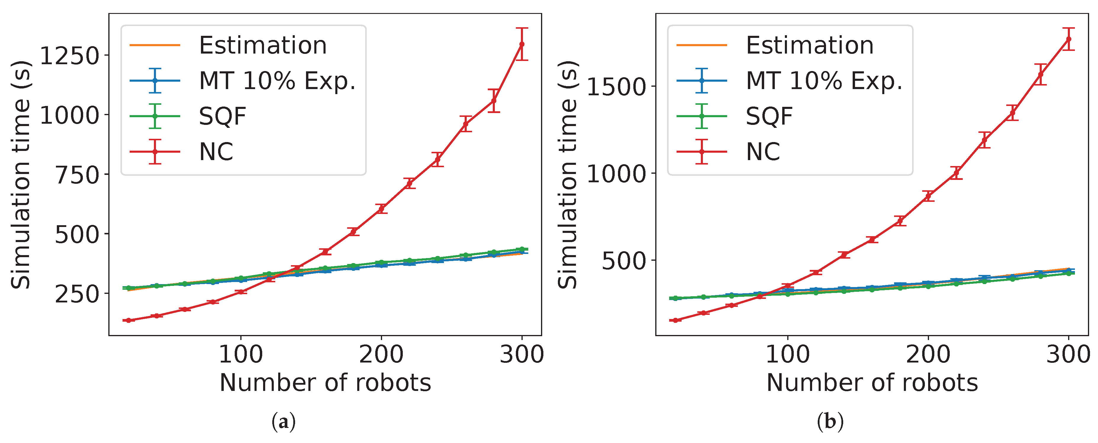
Figure 36.
Comparison of the estimated expected time and the experimental data for MT with NC as group A’s algorithm, group B is executing the TRVF algorithm and for (a) holonomic robots ( and ) and (b) non-holonomic robots ( and ).
Figure 36.
Comparison of the estimated expected time and the experimental data for MT with NC as group A’s algorithm, group B is executing the TRVF algorithm and for (a) holonomic robots ( and ) and (b) non-holonomic robots ( and ).
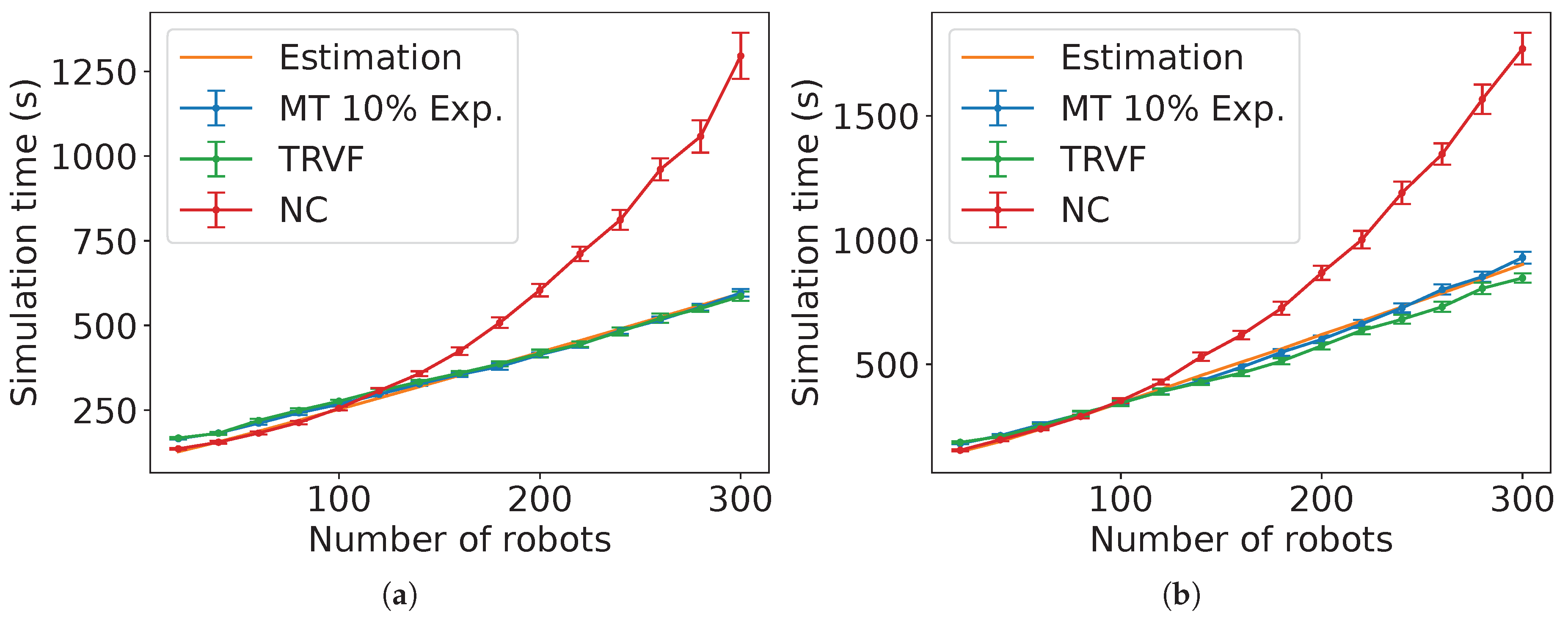
Figure 37.
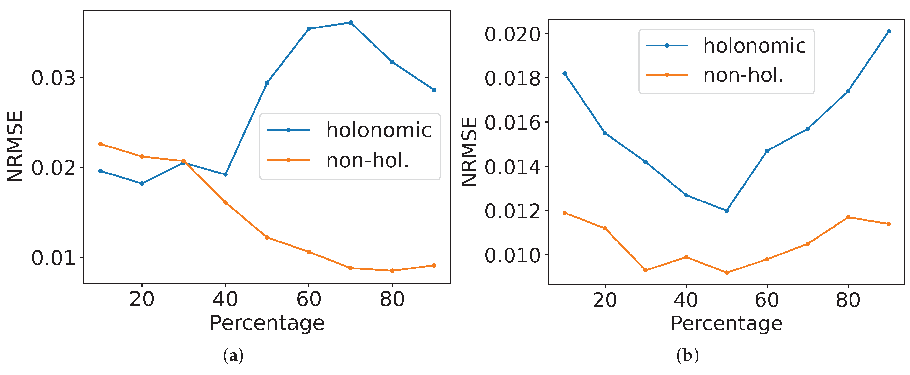
Normalised root mean square error of the estimations with different percentages of robots in group A using NC for an MT with group B using (a) SQF and (b) TRVF.
Figure 37.
Normalised root mean square error of the estimations with different percentages of robots in group A using NC for an MT with group B using (a) SQF and (b) TRVF.
Similarly, Figure 36 shows an example of the estimations for MT with TRVF as control algorithm of group B with . As before, they have the task completion time from the experiments of TRVF and NC for reference. The figures for p ranging from 20% to 90% in steps of 10% appear in Appendix B. Figure 37(b) shows the results of the NRMSE for these estimations. Due to the estimation equation for TRVF working better for a higher number of robots, the ad hoc estimation reflects this result. Also, the NRMSE is higher for holonomic case.
Figure 38 displays the change in constants and by the experimented percentage of robots in group A shown above for each tested control algorithm of the robots in group B and robots’ movement type. Note that when rises, decreases because it is expected that these constants are proportional to the number of robots executing the algorithm associated with each of them. Although the values of the constants are different, the trend for the SQF algorithm is similar for both robots’ movement types (Figure 38(a)). The same happens for the TRVF algorithm in Figure 38(b).
5. Discussion
In this section, limitations, challenges and future improvements to the presented work are discussed. Firstly, this paper assumes that the only random operation is the initial position of the robots. Aside from that, the robots would behave deterministically. Therefore, the average task completion is due to the random initialisation. Thus, a best/worst-case scenario may be estimated by taking the standard deviation from above and below the average time in most cases. Although this is true for the simulations discussed in this paper, for real robots, there would be more stochastic events that should be inputted in these best-case/worst-case scenarios.
Secondly, the presented estimations are valid for changes in the parameters N and s as tested and described in Section 4. However, the estimations were not experimented with different values of every global parameter other than N and s (Table 2). The authors believe the estimations work for reasonable changes in the other global parameters. Nonetheless, significant changes were not tested and could cause unexpected results, since the underlying algorithms could have undesired behaviour with a wrong parametrisation.
Thirdly, the presented algorithms may be adapted to three-dimensional robots and experimented with their type of movements due to the recently increasing usage of aerial robots. Because this paper considered robots and the target regions in a plane, the equations must be extended to three dimensions. Three-dimensional robots have different types of movement that may influence the presented algorithms differently. For instance, aircraft-like robots cannot stop in mid-air, and some aerial robots are controlled by Dubins paths.
In addition, adapting a method made for a space with a fixed number of dimensions may not be effortless. The algorithms SQF and TRVF were born from a tentative by the authors to apply the queuing theory. However, this was unsuccessful because, in two-dimensional space, the queues behave differently depending on the path followed by the robots. In other words, the original queuing theory is one-dimensional, and adapting to two dimensions did not seem to be straightforward. Thus, only extending the algorithms may not be sufficient, but they also must be tested for feasibility. Should the extended algorithms be ineffective in three dimensions, new algorithms ought to be devised.
Another future step is to apply methods from statistical mechanics, in special for many-body problems, to this problem and to compare with those developed here. Such solutions may help to find a potential field that minimises the relation of the task completion time versus the number of robots. Additionally, these studies may answer whether finding such a potential field is possible. Notice that if this is possible, a time relation for a given field has to be given to be minimised, and this work focused on approximating such relation by exploring the usage of the geometry of the overall behaviour of the robots. These ideas are the basis for future improvements, which include finding a better potential field minimising the task completion time per number of robots, presuming that finding it is decidable.
Finally, the method of analysing the geometric behaviour from the experiments to approximate local-to-global functions used here may be applied to different problems of robotic swarms if a fixed number of robots follow similar paths on average for different starting positions. For instance, a patrolling swarm may go to specific areas regularly using a predefined route on average. By aggregating the routes, analysing their geometry and averaging by the frequency of usage, the expected time between patrols may be estimated. A similar analysis may be performed on a swarm covering an area to estimate the average time for completing that task. Another example is to approximate the volume per time of a swarm collecting waste by calculating the average time of collecting and accessing the areas with waste and the volume of waste from them by geometrically examining the used paths from the experiments and averaging by their frequency.
6. Conclusions
This paper presented estimations of the expected task completion time in relation to the number of robots in algorithms for the common target problem using potential fields. These relations were calculated by analysing the experiments with NC, SQF, TRVF and MT. Experiments with MT of two groups showed that if the percentage of robots in one group is lower than 30% and 60% for non-holonomic and holonomic robots, respectively, the results on the average total simulation time are better for NC as algorithm of a group, although it is not suitable for a swarm with only one group.
Besides the number of robots, the expected task completion time estimations are also expressed in terms of the average speed of the robots and algorithm parameters such as the working area radius, the target area radius, the number of lanes in TRVF, its central angle, the distance travelled through its lanes and the ratio of the number of robots in group A to the total number of individuals. In addition, the experimental relation of the average speed and distance between the robots as a function of the number of individuals in the swarm for SQF and TRVF was illustrated.
Therefore, this work is a fundamental first step to examining the common target problem as a local-to-global analysis of the task completion time from the specification of the individual robot to the swarm behaviour. An extensive and challenging study is needed to explain the local-to-global nature of these subsumed details. This invokes a theory to untangle this relationship, and this paper aims to start a discussion about that by presenting a baseline approximation to compare with future work. There is room for improvement on these estimations. Approaches using adaptations of the methods discussed in Section 2 (the perturbation theory, the coupled cluster technique, the density-functional theory, the mean-field theory and the variational method) are welcome to be compared.
Author Contributions
Y.T.P. and L.S.M. wrote the main manuscript. Y.T.P. wrote the source codes, executed the experiments and prepared the figures. Y.T.P. and L.S.M. reviewed the manuscript. Conceptualization, Y.T.P. and L.S.M.; methodology, Y.T.P. and L.S.M.; software, Y.T.P.; validation, Y.T.P.; formal analysis, Y.T.P.; investigation, Y.T.P.; data curation, Y.T.P.; resources, Y.T.P. and L.S.M.; writing–original draft preparation, Y.T.P.; writing–review and editing, Y.T.P. and L.S.M.; visualisation, Y.T.P.; supervision, L.S.M.; project administration, Y.T.P. and L.S.M.; funding acquisition, Y.T.P. and L.S.M.; All authors have read and agreed to the published version of the manuscript.
Funding
This research was funded by the Faculty of Science and Technology (FST) of Lancaster University.
Institutional Review Board Statement
Not applicable.
Informed Consent Statement
Not applicable.
Data Availability Statement
The source codes of the experimented algorithms and estimations are in https://github.com/yuri-tavares/swarm-ad-hoc-follower.
Acknowledgments
This research was funded by the Faculty of Science and Technology (FST) of Lancaster University. Thanks to Gao Peng and Abdulrahman Kerim for the review of the earlier draft.
Conflicts of Interest
The authors declare no conflicts of interest.
Appendix A. Parameter Alg of Mixed Teams
This section presents the results of using combinations of NC, SQF and TRVF by the two groups in an MT and different values of , justifying the usage of = NC in Section 3.4. In the following sections, a fixed algorithm is set for the group B and the usage of different algorithms for the group A is compared by varying the number of robots and the ratio of robots in group A to the total number of robots . Based on the results of Sections Appendix A.1 and Appendix A.2, Appendix A.3 summarises the reason for choosing = NC.
Appendix A.1. Comparison of NC and SQF for the Group A and TRVF for Group B
Figure A1–Figure A3 illustrate the comparison of the total simulation time per total number of robots of an MT using SQF and NC as parameter with percentages of robots in group A to the total number of individuals ranging from 10% to 90% in steps of 10%. In these experiments, TRVF is the swarm control algorithm of group B. These figures are summarised in Figure A4, which shows the sum of the average total simulation time over each experimented number of robots by the percentage of robots in group A for MT. The bars correspond to the respective sum of the confidence interval ranges with .
Figure A1.
Comparison of the total simulation time by the number of robots for the experiments with MT using TRVF as the group B’s algorithm and SQF and NC as the group A’s algorithm by 10% of the robots for (a) holonomic and (b) non-holonomic robots, 20% for (c) holonomic and (d) non-holonomic robots and 30% for (e) holonomic and (f) non-holonomic robots.
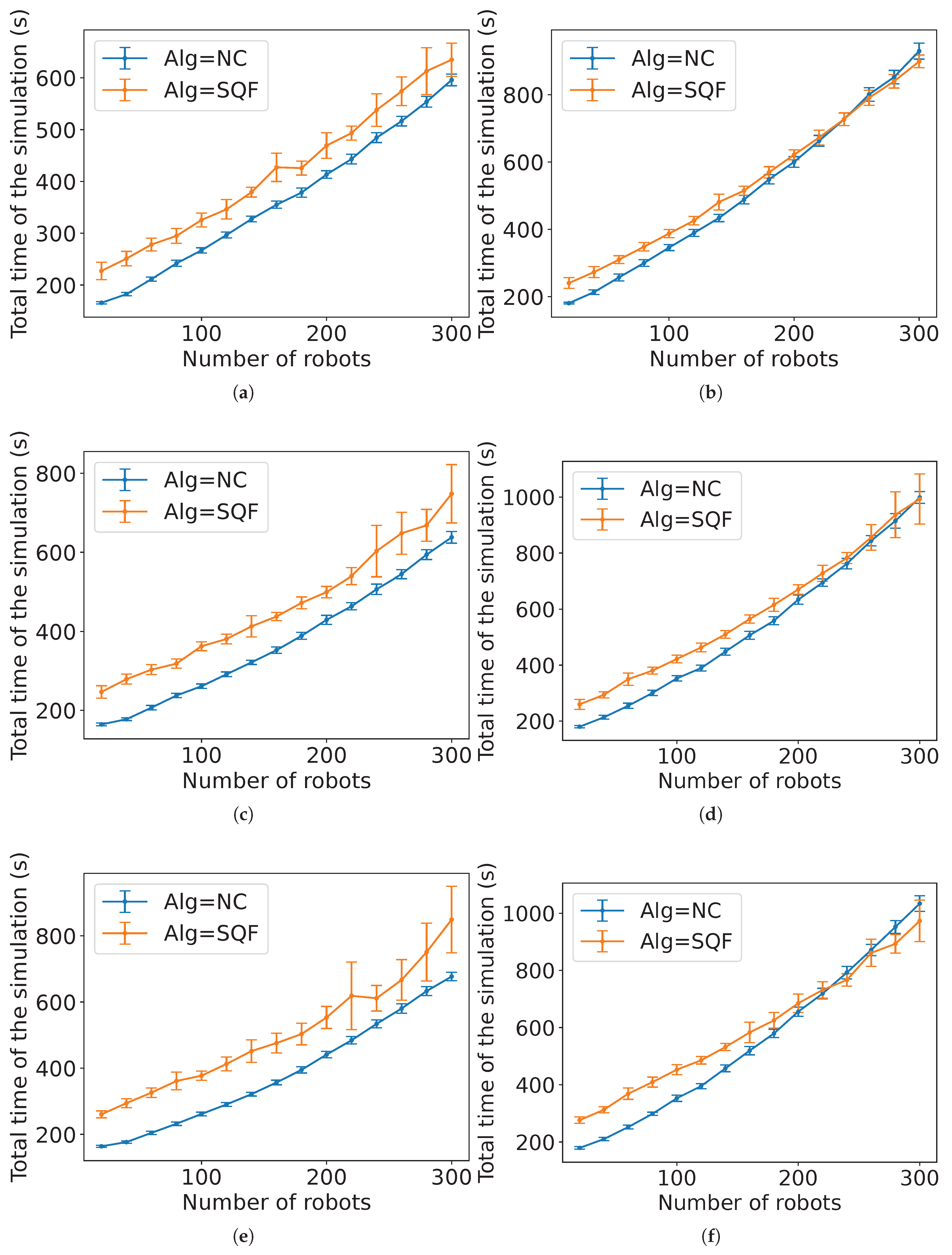
Figure A2.
Comparison of the total simulation time by the number of robots for the experiments with MT using TRVF as the group B’s algorithm and SQF and NC as the group A’s algorithm by 40% of the robots for (a) holonomic and (b) non-holonomic robots, 50% for (c) holonomic and (d) non-holonomic robots and 60% for (e) holonomic and (f) non-holonomic robots.
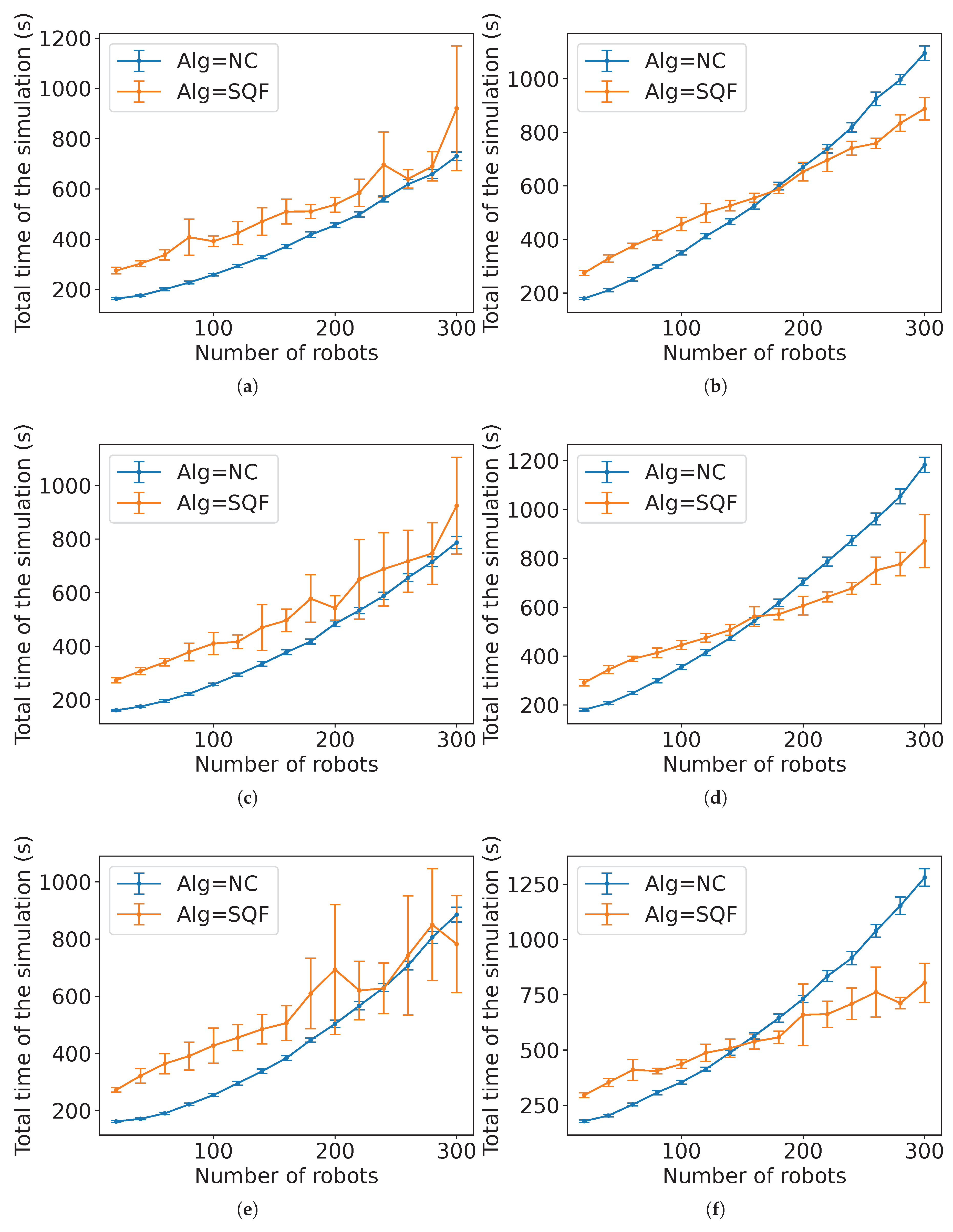
Figure A3.
Comparison of the total simulation time by the number of robots for the experiments with MT using TRVF as the group B’s algorithm and SQF and NC as the group A’s algorithm by 70% of the robots for (a) holonomic and (b) non-holonomic robots, 80% for (c) holonomic and (d) non-holonomic robots and 90% for (e) holonomic and (f) non-holonomic robots.
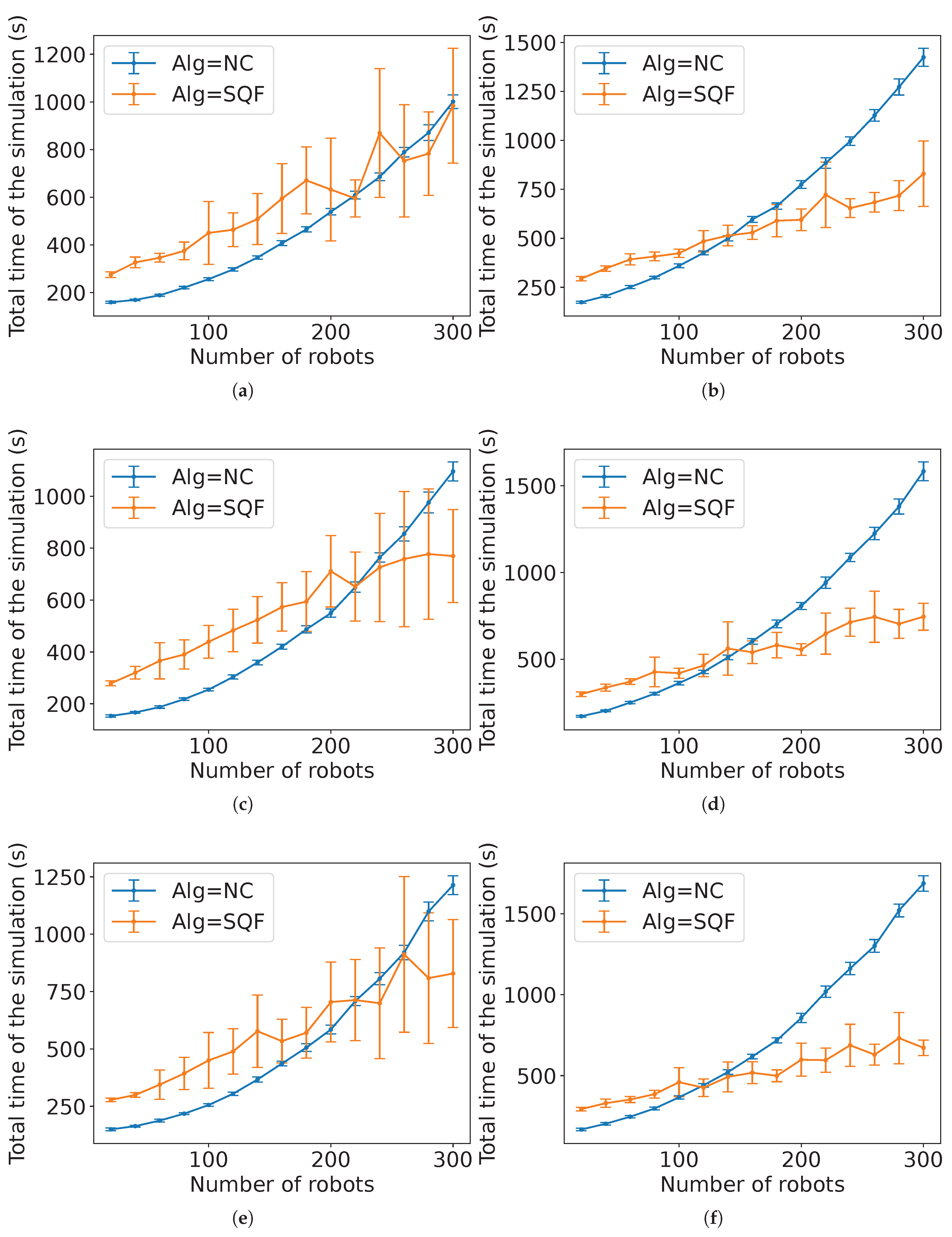
Figure A4.
Comparison of the total simulation time sum over the number of robots by the percentage of robots in group A using NC and SQF as group A’s algorithms. The swarm control algorithm of the robots in group B is TRVF. (a) Holonomic robots. (b) Non-holonomic robots.
Figure A4.
Comparison of the total simulation time sum over the number of robots by the percentage of robots in group A using NC and SQF as group A’s algorithms. The swarm control algorithm of the robots in group B is TRVF. (a) Holonomic robots. (b) Non-holonomic robots.
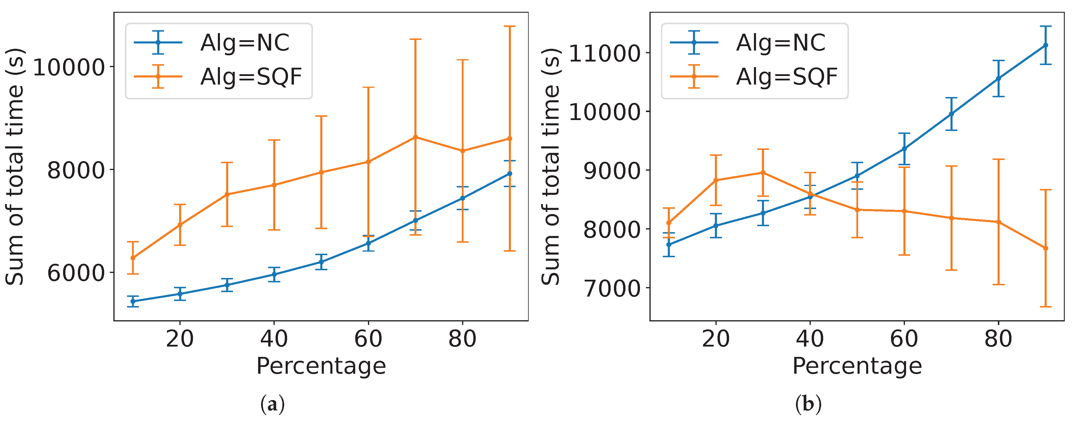
In Figure A1–Figure A3, for 30% to 70% for non-holonomic robots, NC as the algorithm of group A is significantly better on average until different values from 120 to 180 robots. Note that the number of robots where it starts to take less time decreases with the ratio of robots in group A.
Furthermore, SQF as the group A algorithm takes more or equal time on average than using NC for percentages from 10% to 20% of robots in group A using MT for both type of robots and 30% to 70% for holonomic robots with statistical significance (Figure A4). Although the SQF is faster, when used as the group A algorithm for a low percentage of robots, they follow a trajectory longer than they would if NC is in use. As fewer robots are going directly to the target region and there is less congestion, NC is better for low percentages. The variance is higher for SQF because the SQF robots leaving the target area may push the robots using TRVF away from the working area in the bottom lane for a long time.
Additionally, the usage of holonomic robots takes more time and varies more than non-holonomic robots for the SQF algorithm. Holonomic robots are faster to be repelled by another robot due to their lack of restrictions on moving in any direction. Because they can be repelled for longer periods, they tend to take more time going away from the working area.
Appendix A.2. Comparison of NC and TRVF for the Group A and SQF for Group B
Figure A5–Figure A7 show the comparison of NC and TRVF as the group A algorithms for ratios varying from 10% to 90% in steps of 10% for holonomic and non-holonomic robots. In these experiments, SQF is the swarm control algorithm of group B. As before, these figures are summarised in Figure A8, which presents the sum over the number of robots of the average total simulation time by the ratio of robots in group A.
Figure A5.
Comparison of the total simulation time by the number of robots for the experiments with MT using SQF as the group B’s algorithm and TRVF and NC as the group A’s algorithm by 10% of the robots for (a) holonomic and (b) non-holonomic robots, 20% for (c) holonomic and (d) non-holonomic robots and 30% for (e) holonomic and (f) non-holonomic robots.
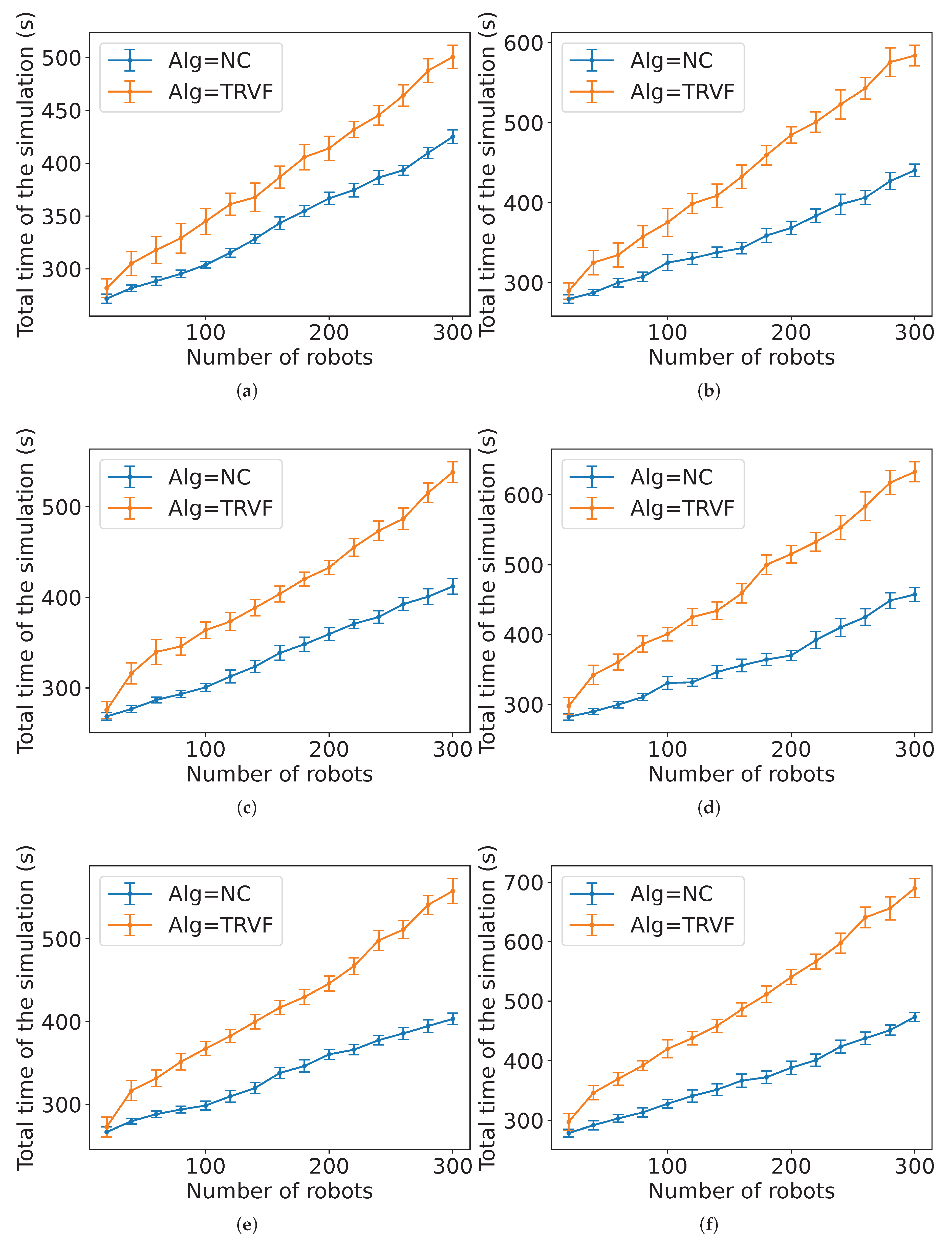
Figure A6.
Comparison of the total simulation time by the number of robots for the experiments with MT using SQF as the group B’s algorithm and TRVF and NC as the group A’s algorithm by 40% of the robots for (a) holonomic and (b) non-holonomic robots, 50% for (c) holonomic and (d) non-holonomic robots and 60% for (e) holonomic and (f) non-holonomic robots.
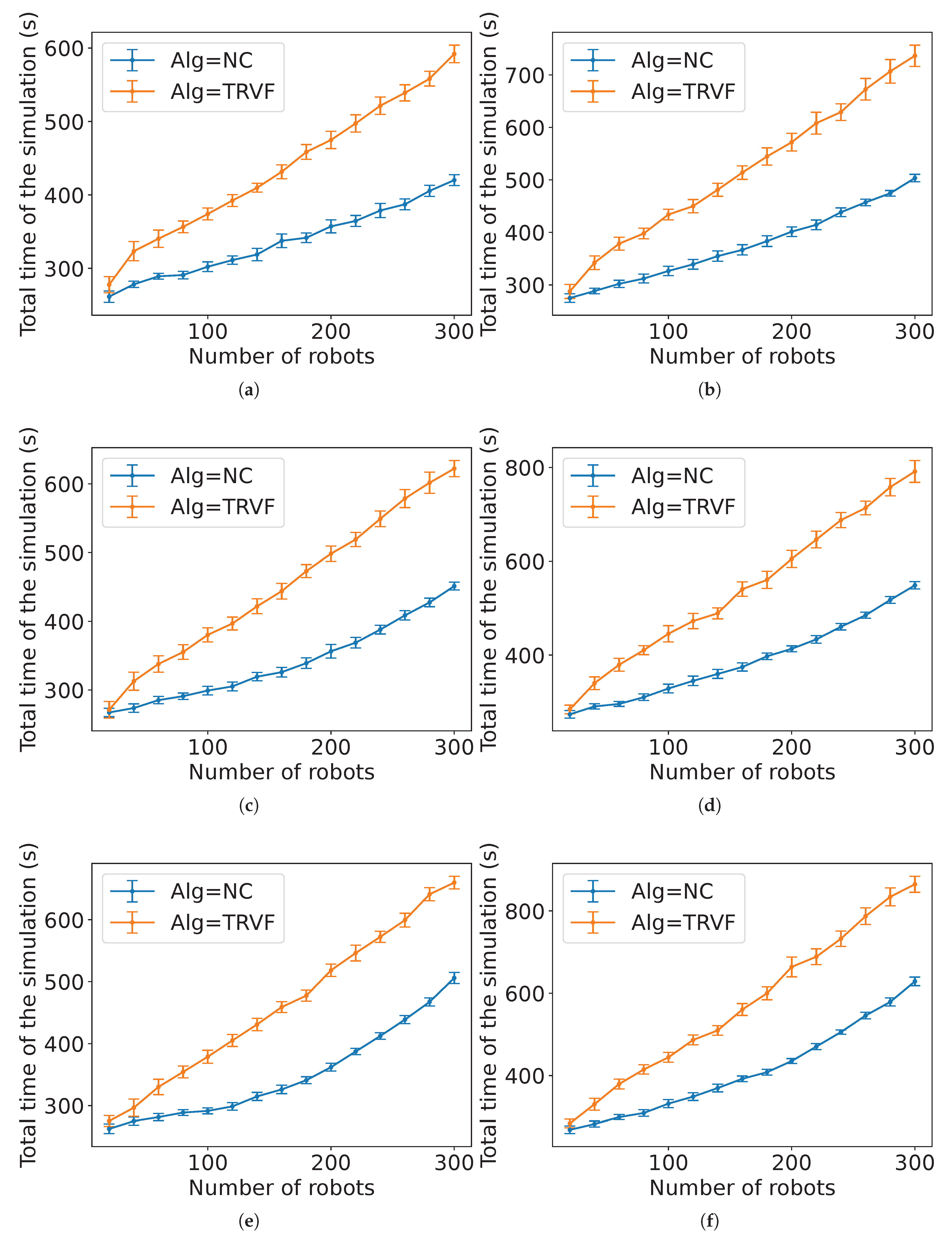
Figure A7.
Comparison of the total simulation time by the number of robots for the experiments with MT using SQF as the group B’s algorithm and TRVF and NC as the group A’s algorithm by 70% of the robots for (a) holonomic and (b) non-holonomic robots, 80% for (c) holonomic and (d) non-holonomic robots and 90% for (e) holonomic and (f) non-holonomic robots.
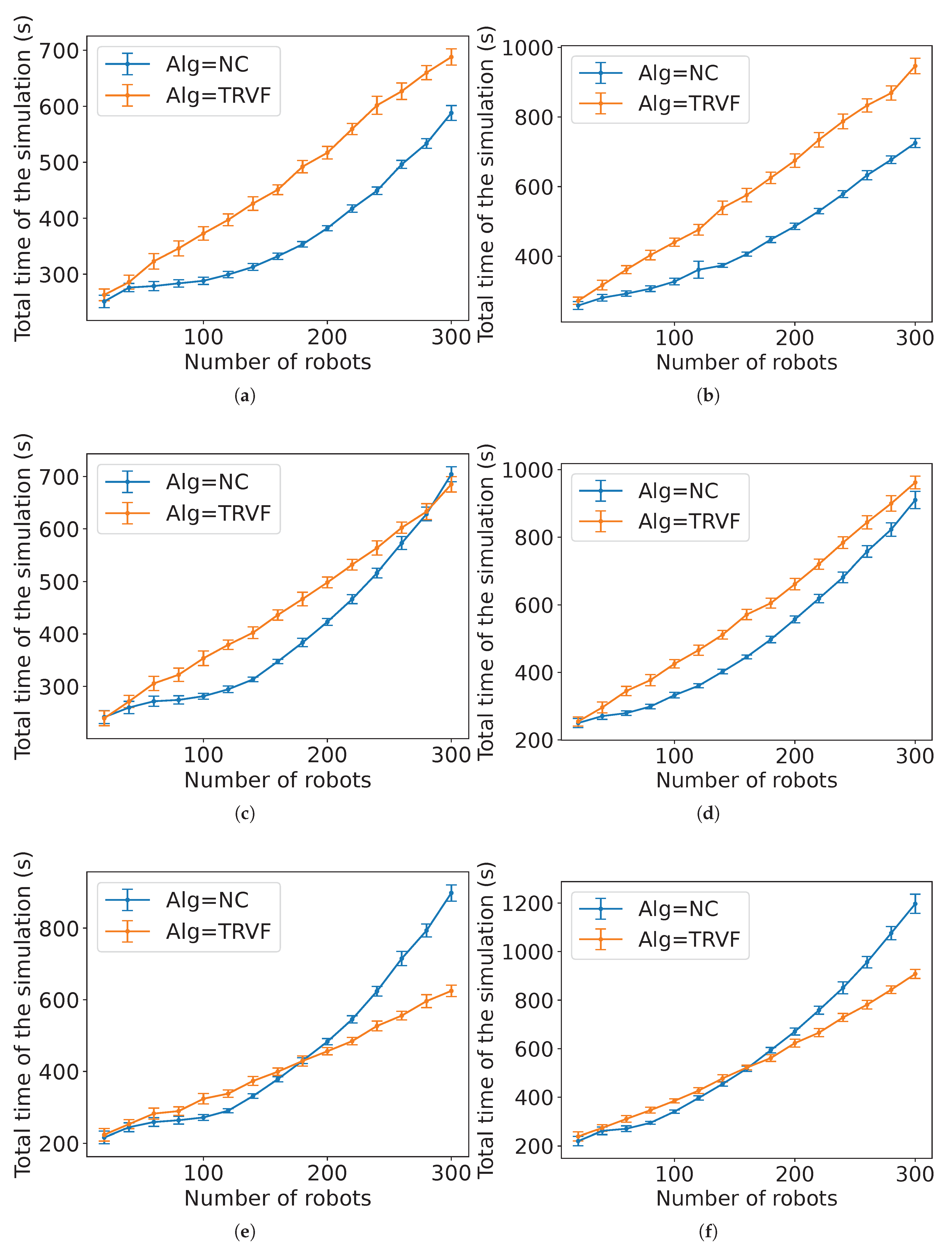
Figure A8.
Comparison of the total simulation time sum over the number of robots by the percentage of robots in group A using NC and TRVF as group A’s algorithms. The swarm control algorithm of the robots in group B is SQF. (a) Holonomic robots. (b) Non-holonomic robots.
Figure A8.
Comparison of the total simulation time sum over the number of robots by the percentage of robots in group A using NC and TRVF as group A’s algorithms. The swarm control algorithm of the robots in group B is SQF. (a) Holonomic robots. (b) Non-holonomic robots.
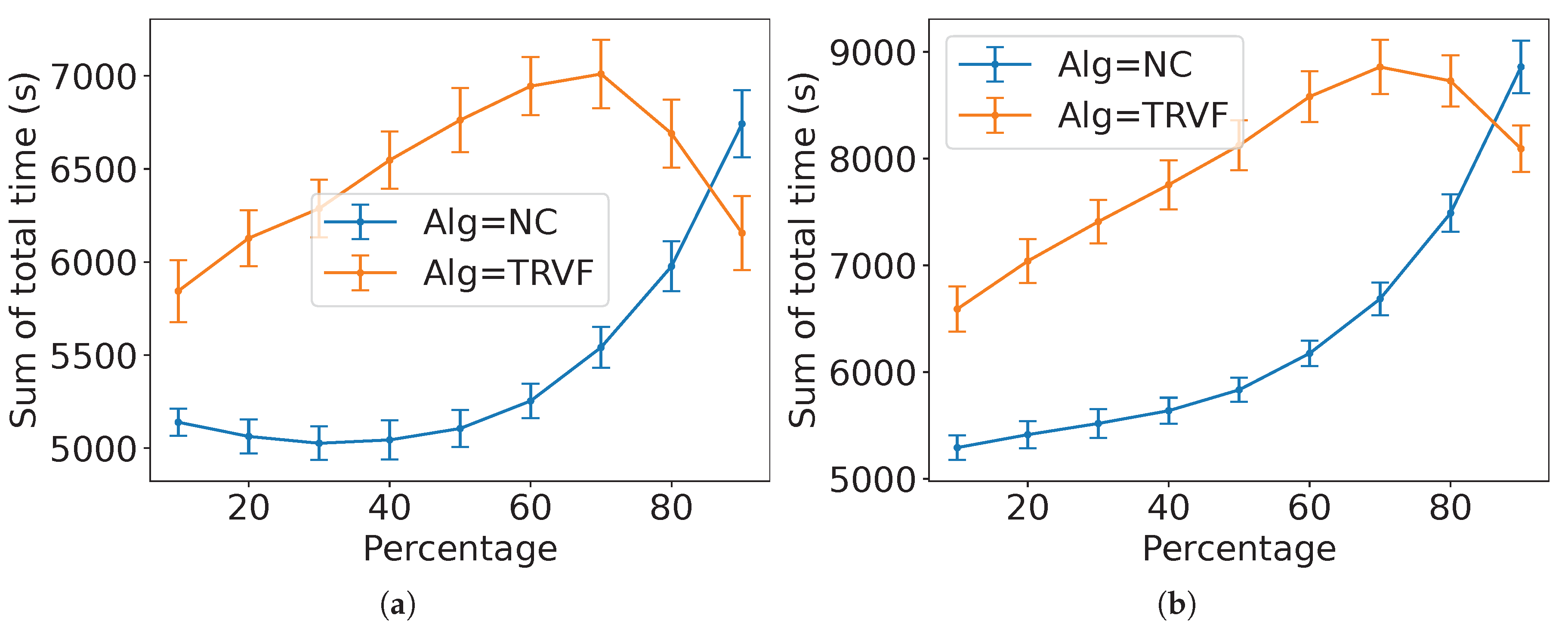
From Figure A7, for 90%, TRVF is significantly better only from 200 to 300 in the holonomic case and from 180 to 300 robots in the non-holonomic cases, respectively. When using the TRVF as an group A algorithm, the lanes near the leaving trajectory of the SQF algorithm create congestion. However, with NC, they tend to go directly to the target, opening space near the SQF leaving area.
In addition, from Figure A8, NC as the group A algorithm takes less or equal time than using TRVF on average for percentages from 10% to 80% for both types of robots with statistical significance.
Appendix A.3. Selection of Alg = NC
Based on the results of Appendix A.1 and Appendix A.2, although NC is the slowest algorithm for handling the common target problem for numerous robots [8], it was the best group A algorithm in most cases with statistical significance. Therefore, NC was selected as the default group A algorithm in the experiments. In addition, MT are expected to be used for small ratios of robots in group A when assuming it would be made of auxiliary robots not knowing the control algorithm of the other group in an ad hoc teamwork scenario. Remember, however, that SQF and TRVF still outperform NC for this problem as the swarm control algorithm [23], and the results only relate to the choice of group A’s algorithm. Nevertheless, if the proportion of robots in group A and an estimated number of robots are known beforehand, the group A algorithm can be chosen based on the graphs.
Appendix B. Additional Graphs
Figure A9–Figure A11 present estimations for MT with the proportion p of robots in group A from 20% to 90% in increments of 10% and SQF as the control algorithm of the robots in group B.
Figure A9.
Comparison of the estimated expected time and the experimental data for MT with NC as group A’s algorithm, group B is executing the SQF algorithm, for (a) holonomic robots ( and ) and (b) non-holonomic robots ( and ), for (c) holonomic robots ( and ) and (d) non-holonomic robots ( and ) and for (e) holonomic robots ( and ) and (f) non-holonomic robots ( and ).
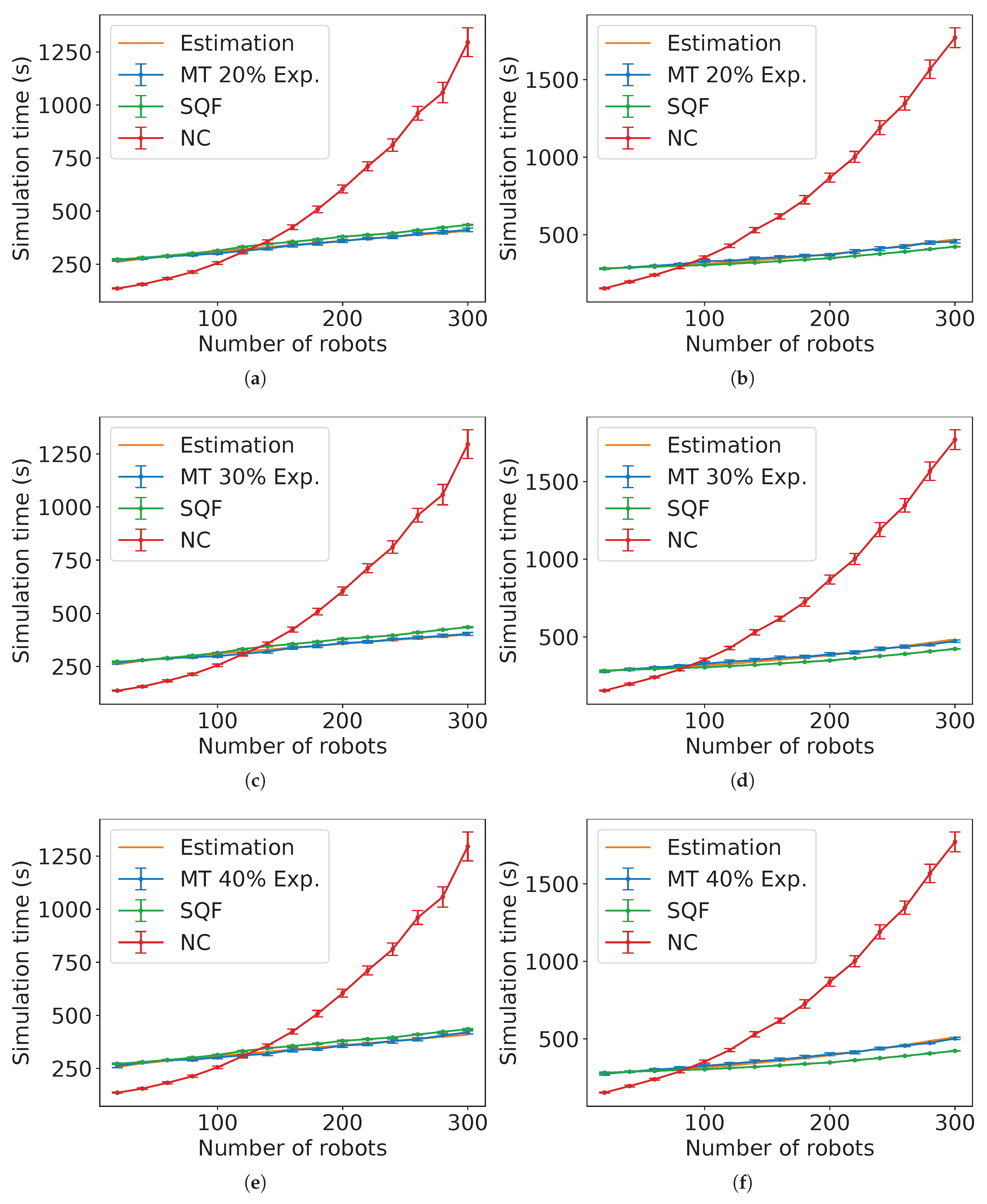
Figure A10.
Comparison of the estimated expected time and the experimental data for MT with NC as group A’s algorithm, group B is executing the SQF algorithm, for (a) holonomic robots ( and ) and (b) non-holonomic robots ( and ), for (c) holonomic robots ( and ) and (d) non-holonomic robots ( and ) and for (e) holonomic robots ( and ) and (f) non-holonomic robots ( and ).
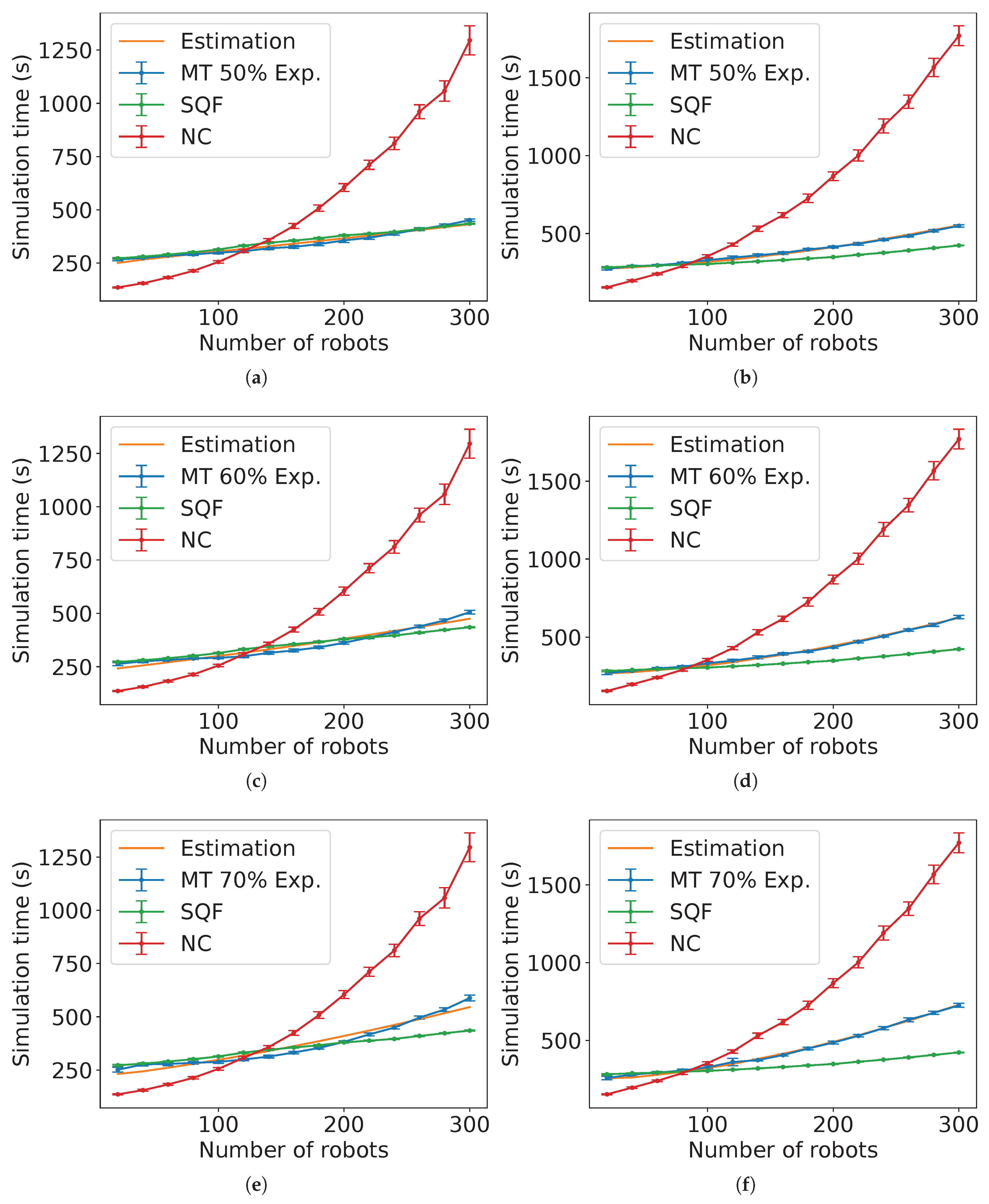
Figure A11.
Comparison of the estimated expected time and the experimental data for MT with NC as group A’s algorithm, , group B is executing the SQF algorithm, for (a) holonomic robots ( and ) and (b) non-holonomic robots ( and ) and for (c) holonomic robots ( and ) and (d) non-holonomic robots ( and ).
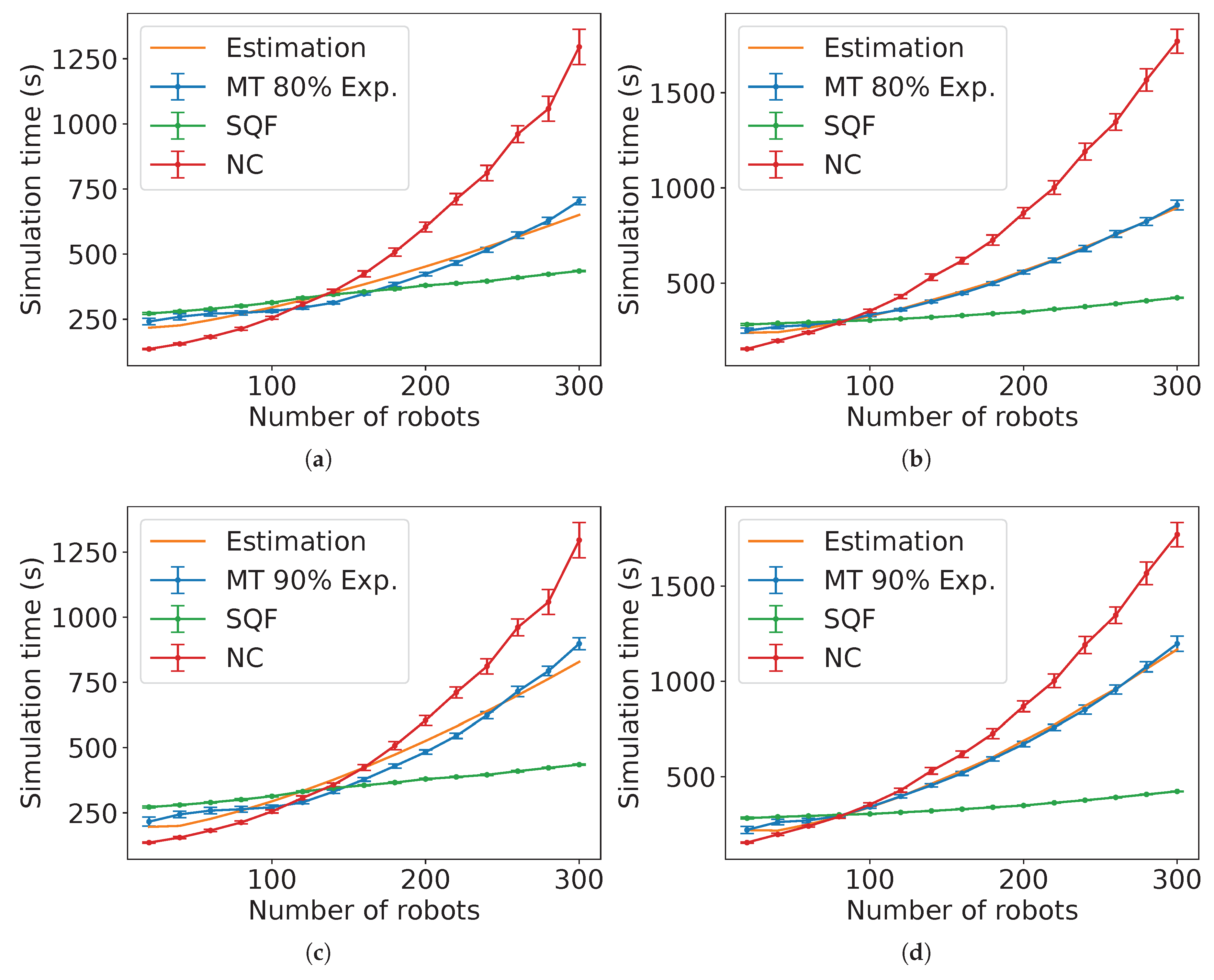
Figure A12–Figure A14 show the estimations for MT with TRVF as control algorithm of group B with p from 20% to 90% in steps of 10%.
Figure A12.
Comparison of the estimated expected time and the experimental data for MT with NC as group A’s algorithm, group B is executing the TRVF algorithm, for (a) holonomic robots ( and ) and (b) non-holonomic robots ( and ), for (c) holonomic robots ( and ) and (d) non-holonomic robots ( and ) and for (e) holonomic robots ( and ) and (f) non-holonomic robots ( and ).
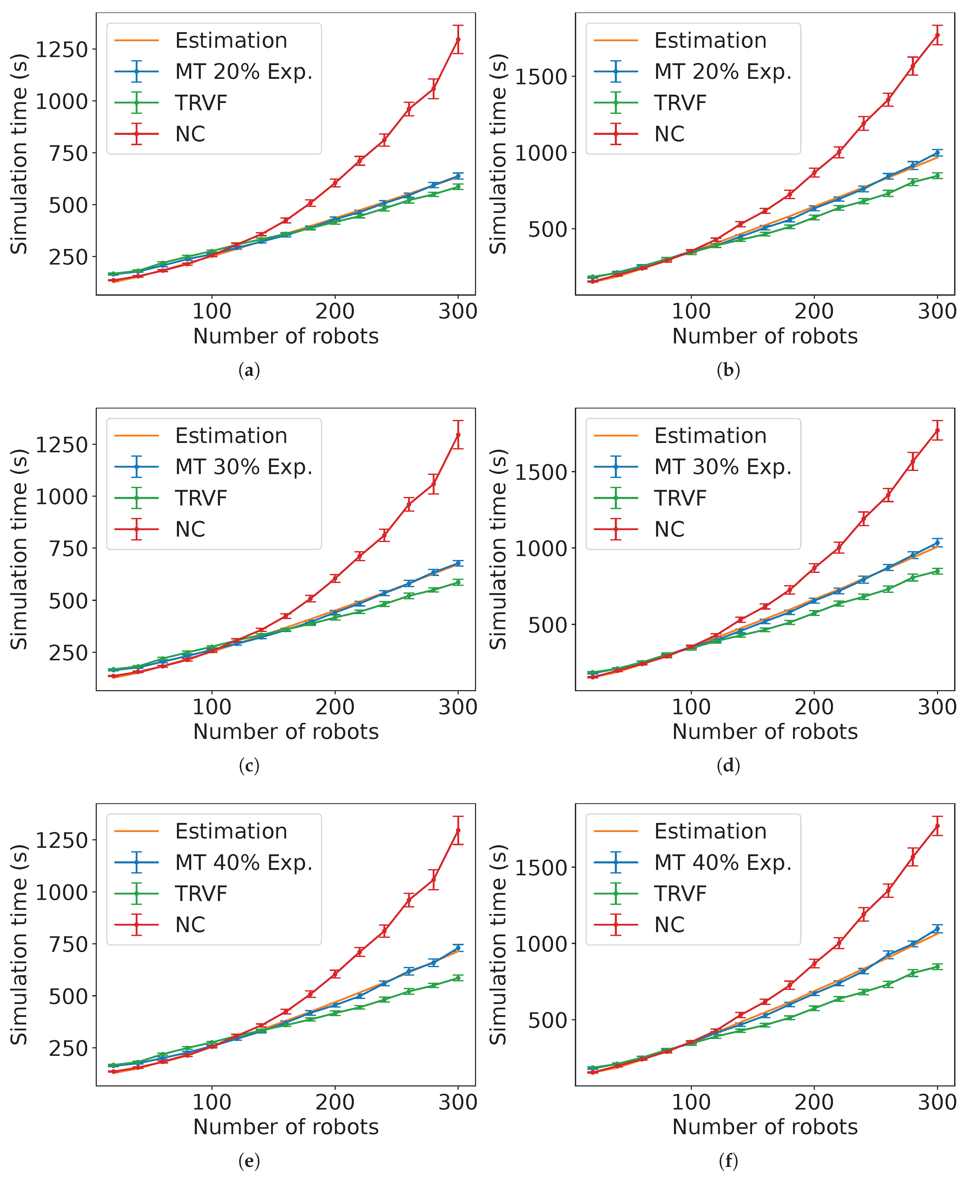
Figure A13.
Comparison of the estimated expected time and the experimental data for MT with NC as group A’s algorithm, group B is executing the TRVF algorithm, for (a) holonomic robots ( and ) and (b) non-holonomic robots ( and ), for (c) holonomic robots ( and ) and (d) non-holonomic robots ( and ) and for (e) holonomic robots ( and ) and (f) non-holonomic robots ( and ).
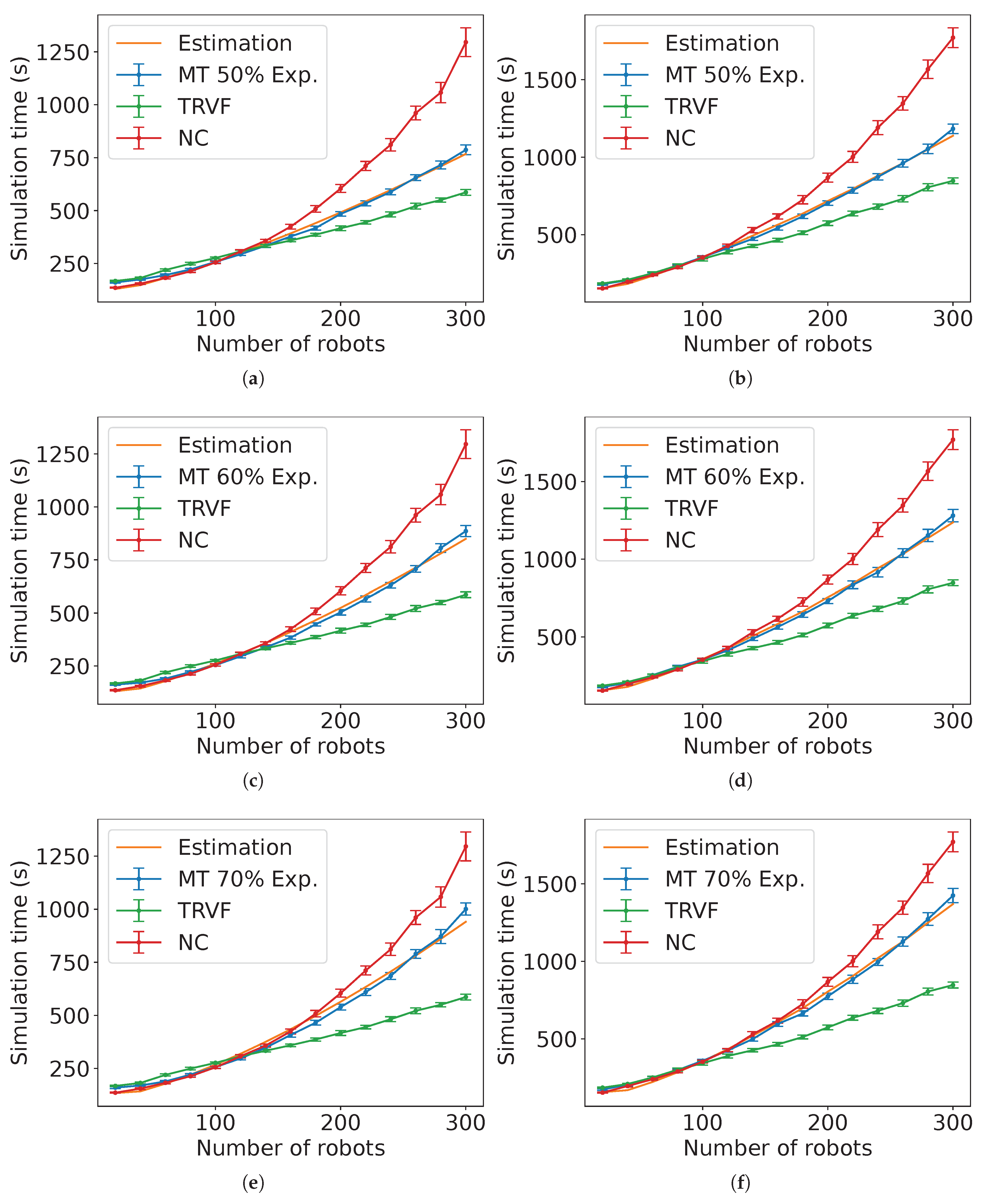
Figure A14.
Comparison of the estimated expected time and the experimental data for MT with NC as group A’s algorithm, group B is executing the TRVF algorithm, for (a) holonomic robots ( and ) and (b) non-holonomic robots ( and ) and for (c) holonomic robots ( and ) and (d) non-holonomic robots ( and ).
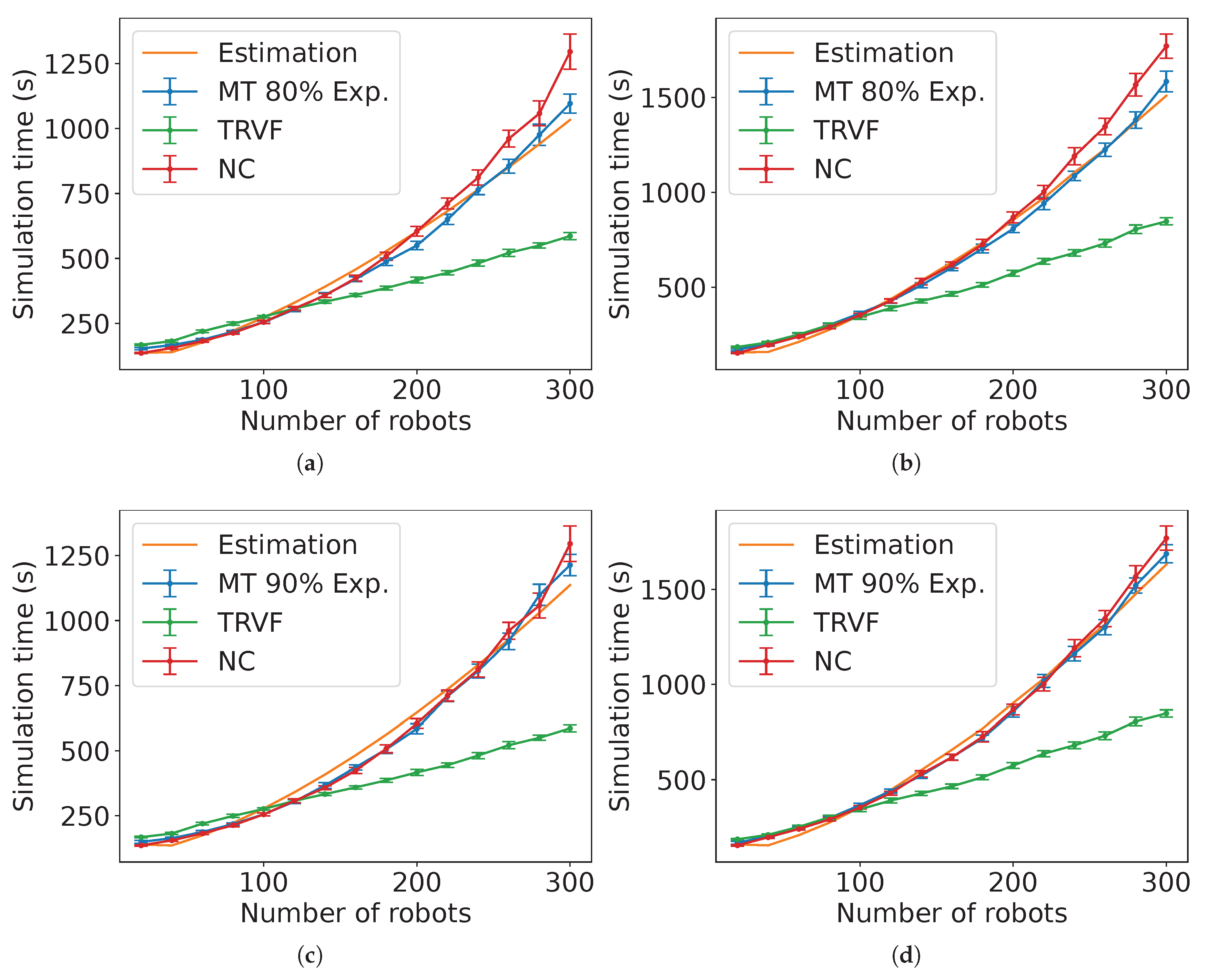
References
- Navarro, I.; Matía, F. An introduction to swarm robotics. International Scholarly Research Notices 2013, 2013. [Google Scholar] [CrossRef]
- Sahin, E. Swarm Robotics: From Sources of Inspiration to Domains of Application. In Proceedings of the International Workshop in Swarm Robotics (SAB); Sahin, E.; Spears, W.M., Eds., Berlin, Heidelberg; 2005; pp. 10–20. [Google Scholar] [CrossRef]
- Beni, G.; Wang, J. Swarm Intelligence in Cellular Robotic Systems. In Proceedings of the NATO Advanced Workshop on Robots and Biological Systems; Dario, P.; Sandini, G.; Aebischer, P., Eds., Berlin, Heidelberg; 1993; pp. 703–712. [Google Scholar] [CrossRef]
- Dudek, G.; Jenkin, M.; Milios, E.; Wilkes, D. A taxonomy for swarm robots. In Proceedings of the IEEE/RSJ International Conference on Intelligent Robots and Systems (IROS), Vol. 1; 1993; pp. 441–447. [Google Scholar] [CrossRef]
- Garnier, S.; Gautrais, J.; Theraulaz, G. The biological principles of swarm intelligence. Swarm Intelligence 2007, 1, 3–31. [Google Scholar] [CrossRef]
- Mataric, M.J. Designing and Understanding Adaptive Group Behavior. Adapt. Behav. 1995, 4, 51–80. [Google Scholar] [CrossRef]
- Panait, L.; Luke, S. Evolving Foraging Behaviors. In Proceedings of the Second International Workshop on the Mathematics and Algorithms of Social Insects; 2003; pp. 131–138. [Google Scholar]
- Marcolino, L.S.; Passos, Y.T.; Souza, A.A.F.d.; Rodrigues, A.d.S.; Chaimowicz, L. Avoiding Target Congestion on the Navigation of Robotic Swarms. Autonomous Robots 2017, 41, 1297–1320. [Google Scholar] [CrossRef]
- Chaudhari, M.S.; Patil, B.; Raut, V. IoT based Waste Collection Management System for Smart Cities: An Overview. In Proceedings of the 3rd International Conference on Computing Methodologies and Communication (ICCMC); 2019; pp. 802–805. [Google Scholar] [CrossRef]
- Mărgăritescu, M.; Ancuța, P.N.; Canale, E.V.; Stanciu, D.I.; Dumitriu, D.; Brișan, C.M. Control of an Autonomous Mobile Waste Collection Robot. In Proceedings of the International Conference of Mechatronics and Cyber - MixMechatronics; Gheorghe, G.I., Ed., Cham; 2020; pp. 51–63. [Google Scholar]
- Costa, L.R.; Aloise, D.; Gianoli, L.G.; Lodi, A. OptiMaP: swarm-powered Optimized 3D Mapping Pipeline for emergency response operations. In Proceedings of the 18th International Conference on Distributed Computing in Sensor Systems (DCOSS); 2022; pp. 269–276. [Google Scholar] [CrossRef]
- Stewart, R.L.; Russell, R.A. A Distributed Feedback Mechanism to Regulate Wall Construction by a Robotic Swarm. Adaptive Behavior 2006, 14, 21–51. [Google Scholar] [CrossRef]
- Liu, J.; Siragam, V.; Gong, Z.; Chen, J.; Fridman, M.D.; Leung, C.; Lu, Z.; Ru, C.; Xie, S.; Luo, J.; et al. Robotic Adherent Cell Injection for Characterizing Cell–Cell Communication. IEEE Transactions on Biomedical Engineering 2015, 62, 119–125. [Google Scholar] [CrossRef]
- Galstyan, A.; Hogg, T.; Lerman, K. Modeling and mathematical analysis of swarms of microscopic robots. In Proceedings of the IEEE Swarm Intelligence Symposium (SIS); 2005; pp. 201–208. [Google Scholar] [CrossRef]
- Bogdan, P.; Wei, G.; Marculescu, R. Modeling populations of micro-robots for biological applications. In Proceedings of the IEEE International Conference on Communications (ICC); 2012; pp. 6188–6192. [Google Scholar] [CrossRef]
- Wang, B.; Liu, D.; Liao, Y.; Huang, Y.; Ni, M.; Wang, M.; Ma, Z.; Wu, Z.; Lu, Y. Spatiotemporally Actuated Hydrogel by Magnetic Swarm Nanorobotics. ACS Nano 2022, 16, 20985–21001. [Google Scholar] [CrossRef] [PubMed]
- Arnold, R.D.; Yamaguchi, H.; Tanaka, T. Search and rescue with autonomous flying robots through behavior-based cooperative intelligence. Journal of International Humanitarian Action 2018, 3, 18. [Google Scholar] [CrossRef]
- Wen, J.; He, L.; Zhu, F. Swarm Robotics Control and Communications: Imminent Challenges for Next Generation Smart Logistics. IEEE Communications Magazine 2018, 56, 102–107. [Google Scholar] [CrossRef]
- Yogi, G.B.; Bhasha, S.M.; Ram, C.S.; Latha, M.P. Swarm Robots for Warehouse Management. International Journal of Research in Engineering, Science and Management 2020, 3, 706–709. [Google Scholar]
- Khaluf, Y.; Dorigo, M. Modeling Robot Swarms Using Integrals of Birth-Death Processes. ACM Trans. Auton. Adapt. Syst. 2016, 11, 8. [Google Scholar] [CrossRef]
- Marcolino, L.S.; Chaimowicz, L. Traffic control for a swarm of robots: Avoiding target congestion. In Proceedings of the IEEE/RSJ International Conference on Intelligent Robots and Systems (IROS); 2009; pp. 1955–1961. [Google Scholar] [CrossRef]
- Passos, Y.T.d.; Duquesne, X.; Marcolino, L.S. On the Throughput of the Common Target Area for Robotic Swarm Strategies. Mathematics 2022, 10, 2482. [Google Scholar] [CrossRef]
- Passos, Y.T.d.; Duquesne, X.; Marcolino, L.S. Congestion control algorithms for robotic swarms with a common target based on the throughput of the target area. Robotics and Autonomous Systems 2023, 159, 104284. [Google Scholar] [CrossRef]
- Cai, Y.; Guo, E.; Li, W.; Gao, H. A Self-organized Circular Formation Algorithm for Planar Robot Swarm. In Proceedings of the 5th Chinese Conference on Swarm Intelligence and Cooperative Control (CCSICC); Ren, Z.; Wang, M.; Hua, Y., Eds., Singapore; 2023; pp. 702–710. [Google Scholar] [CrossRef]
- Barnes, L.; Fields, M.; Valavanis, K. Unmanned ground vehicle swarm formation control using potential fields. In Proceedings of the Mediterranean Conference on Control and Automation (MED); 2007; pp. 1–8. [Google Scholar] [CrossRef]
- Galvez, R.L.; Faelden, G.E.U.; Maningo, J.M.Z.; Nakano, R.C.S.; Dadios, E.P.; Bandala, A.A.; Vicerra, R.R.P.; Fernando, A.H. Obstacle avoidance algorithm for swarm of quadrotor unmanned aerial vehicle using artificial potential fields. In Proceedings of the IEEE Region 10 Conference (TENCON); 2017; pp. 2307–2312. [Google Scholar] [CrossRef]
- Patwardhan, A.; Murai, R.; Davison, A.J. Distributing Collaborative Multi-Robot Planning With Gaussian Belief Propagation. IEEE Robotics and Automation Letters 2023, 8, 552–559. [Google Scholar] [CrossRef]
- Beavers, G.; Hexmoor, H. Teams of agents. In Proceedings of the 2001 IEEE International Conference on Systems, Man and Cybernetics. e-Systems and e-Man for Cybernetics in Cyberspace, Vol. 1; 2001; pp. 574–582. [Google Scholar] [CrossRef]
- dos Santos, R.F.; Ramachandran, R.K.; Vieira, M.A.; Sukhatme, G.S. Parallel multi-speed Pursuit-Evasion Game algorithms. Robotics and Autonomous Systems 2023, 163, 104382. [Google Scholar] [CrossRef]
- Salimi, M.; Ibragimov, G.I.; Siegmund, S.; Sharifi, S. On a Fixed Duration Pursuit Differential Game with Geometric and Integral Constraints. Dynamic Games and Applications 2016, 6, 409–425. [Google Scholar] [CrossRef]
- Flammini, B.; Azzalini, D.; Amigoni, F. Multi-Agent Pickup and Delivery in Presence of Another Team of Robots. In Proceedings of the Proceedings of the 2023 International Conference on Autonomous Agents and Multiagent Systems, 2023, pp.
- Stone, P.; Kaminka, G.A.; Kraus, S.; Rosenschein, J.S. Ad Hoc Autonomous Agent Teams: Collaboration without Pre-Coordination. In Proceedings of the Twenty-Fourth Conference on Artificial Intelligence (AAAI); 7 2010. [Google Scholar] [CrossRef]
- Melo, F.S.; Sardinha, A. Ad Hoc Teamwork by Learning Teammates’ Task. Autonomous Agents and Multi-Agent Systems 2016, 30, 175–219. [Google Scholar] [CrossRef]
- Mirsky, R.; Carlucho, I.; Rahman, A.; Fosong, E.; Macke, W.; Sridharan, M.; Stone, P.; Albrecht, S.V. A Survey of Ad Hoc Teamwork Research. In Proceedings of the 19th European Conference on Multi-Agent Systems (EUMAS); Baumeister, D.; Rothe, J., Eds., Cham; 2022; pp. 275–293. [Google Scholar] [CrossRef]
- Albrecht, S.V.; Stone, P. Autonomous agents modelling other agents: A comprehensive survey and open problems. Artificial Intelligence 2018, 258, 66–95. [Google Scholar] [CrossRef]
- Gerkey, B.P.; Vaughan, R.T.; Howard, A. The Player/Stage Project: Tools for Multi-Robot and Distributed Sensor Systems. In Proceedings of the 11th International Conference on Advanced Robotics (ICAR), ICAR; 2003; pp. 317–323. [Google Scholar]
- Soni, A.; Dasannacharya, C.; Gautam, A.; Shekhawat, V.S.; Mohan, S. Multi-Robot Unknown Area Exploration Using Frontier Trees. In Proceedings of the 2022 IEEE/RSJ International Conference on Intelligent Robots and Systems (IROS); 2022; pp. 9934–9941. [Google Scholar] [CrossRef]
- Calderón-Arce, C.; Brenes-Torres, J.C.; Solis-Ortega, R. Swarm Robotics: Simulators, Platforms and Applications Review. Computation 2022, 10. [Google Scholar] [CrossRef]
- Miteva, L.; Yovchev, K.; Chikurtev, D. Software and Hardware Infrastructure for Research and Development of Intelligent Control for Robotic Manipulators. In Proceedings of the 2022 XXXI International Scientific Conference Electronics (ET); 2022; pp. 1–5. [Google Scholar] [CrossRef]
- Boogerd, F.C.; Bruggeman, F.J.; Richardson, R.C.; Stephan, A.; Westerhoff, H.V. Emergence and Its Place in Nature: A Case Study of Biochemical Networks. Synthese 2005, 145, 131–164. [Google Scholar] [CrossRef]
- Holland, J.H. Emergence: from Chaos to Order; Oxford University Press: United Kingdom, 1998. [Google Scholar]
- Feltz, B.; Crommelinck, M.; Goujon, P. Self-organization and Emergence in Life Sciences; Synthese Library, Springer Netherlands: Netherlands, 2006. [Google Scholar]
- Couzin, I. Geometric Principles of Individual and Collective Decision-Making. Keynote talk presented at the 22nd International Conference on Autonomous Agents and Multiagent Systems (AAMAS-2023), 2023. https://www.southampton.ac.uk/~eg/AAMAS2023/pdfs/p3.pdf. Accessed on 11 July 2023. [Google Scholar]
- Haken, H. Synergetics: An Introduction : Nonequilibrium Phase Transitions and Self-organization in Physics, Chemistry, and Biology; Springer: Germany, 1983. [Google Scholar]
- March, N.; Young, W.; Sampanthar, S. The Many-Body Problem in Quantum Mechanics; Dover books on physics, Dover Publications: United Kingdom, 1995. [Google Scholar]
- Kuzemsky, A. Statistical Mechanics And The Physics Of Many-particle Model Systems; World Scientific Publishing Company: Digital, 2017. [Google Scholar]
- Mandl, F. Statistical Physics; Manchester physics series; Wiley: United Kingdom, 1971. [Google Scholar]
- Huang, K. Statistical Mechanics, 2 ed.; John Wiley & Sons: Canada, 1987. [Google Scholar]
- Kato, T. A Short Introduction to Perturbation Theory for Linear Operators; Springer New York: New York, 2012. [Google Scholar]
- Holmes, M. Introduction to Perturbation Methods; Texts in Applied Mathematics, Springer New York: New York, 1998. [Google Scholar]
- Bartlett, R.J.; Musiał, M. Coupled-cluster theory in quantum chemistry. Rev. Mod. Phys. 2007, 79, 291–352. [Google Scholar] [CrossRef]
- Shavitt, I.; Bartlett, R. Many-Body Methods in Chemistry and Physics: MBPT and Coupled-Cluster Theory; Cambridge Molecular Science, Cambridge University Press: United Kingdom, 2009. [Google Scholar]
- Glossman-Mitnik, D. Density Functional Theory; IntechOpen: Digital, 2019. [Google Scholar]
- Dreizler, R.M.; Gross, E.K.U. Density functional theory; NATO ASI series. Series B, Physics, Ed.; v. 337, Plenum Press: New York, 1995. [Google Scholar]
- Opper, M.; Saad, D. Advanced Mean Field Methods: Theory and Practice; Neural information processing series; MIT Press: USA, 2001. [Google Scholar]
- Chen, Y.; Georgiou, T.T.; Pavon, M. Steering the Distribution of Agents in Mean-Field Games System. Journal of Optimization Theory and Applications 2018, 179, 332–357. [Google Scholar] [CrossRef]
- Lasry, J.M.; Lions, P.L. Mean field games. Japanese Journal of Mathematics 2007, 2, 229–260. [Google Scholar] [CrossRef]
- Jiao, C.; Liang, J.C.; Yu, Z.F.; Chen, Y.; Zhang, A.X.; Xue, J.K. Bose—Einstein condensates with tunable spin—orbit coupling in the two-dimensional harmonic potential: The ground-state phases, stability phase diagram and collapse dynamics. Frontiers of Physics 2022, 17, 61503. [Google Scholar] [CrossRef]
- Pérez-Torres, J.F. Dilemma of the “Best Wavefunction”: Comparing Results of the STO-NG Procedure versus the Linear Variational Method. Journal of Chemical Education 2019, 96, 704–707. [Google Scholar] [CrossRef]
- Carleo, G.; Troyer, M. Solving the quantum many-body problem with artificial neural networks. Science 2017, 355, 602–606. [Google Scholar] [CrossRef]
- Hamann, H. Swarm Robotics: A Formal Approach; Springer: Germany, 2018. [Google Scholar]
- Prigogine, I.; Andrews, F.C. A Boltzmann-Like Approach for Traffic Flow. Operations Research 1960, 8, 789–797. [Google Scholar] [CrossRef]
- Iannini, M.L.L.; Dickman, R. Kinetic theory of vehicular traffic. American Journal of Physics 2016, 84, 135–145. [Google Scholar] [CrossRef]
- Prigogine, I.; Herman, R. Kinetic Theory of Vehicular Traffic; Elsevier: New York, 1971. [Google Scholar]
- Elamvazhuthi, K.; Berman, S. Mean-field models in swarm robotics: a survey. Bioinspiration & Biomimetics 2019, 15, 015001. [Google Scholar] [CrossRef]
- Morin, D. Introduction to classical mechanics : with problems and solutions; Cambridge University Press: Cambridge, United Kingdom, 2007; p. 719. [Google Scholar]
- Siegwart, R.; Nourbakhsh, I.R. Introduction to Autonomous Mobile Robots; Bradford Company: Scituate, MA, USA, 2004. [Google Scholar]
- Casella, G.; Berger, R. Statistical Inference, ed., 2nd ed.; Duxbury – Thomson Learning: USA, 2002. [Google Scholar]
- Nelson, D.; Barber, D.; McLain, T.; Beard, R. Vector field path following for small unmanned air vehicles. In Proceedings of the American Control Conference (ACC); 2006; pp. 5788–5794. [Google Scholar] [CrossRef]
| 1 | In this work, bold is for points located at a previously defined position vector and non-bold for those not associated with such a vector. |
| 2 | The source codes of the experimented algorithms and estimations are in https://github.com/yuri-tavares/swarm-ad-hoc-follower. |
Figure 1.
Example of an experiment of the NC algorithm with and default values. (a) Start of the experiment. (b) The first robot to reach the target area. (c) More robots reach the target region, fill this area and try to leave. (d) Queues of robots formed to leave the cluttered area. Full simulation available on https://youtu.be/qgLxFk0OGyo, accessed on 14 October 2022.
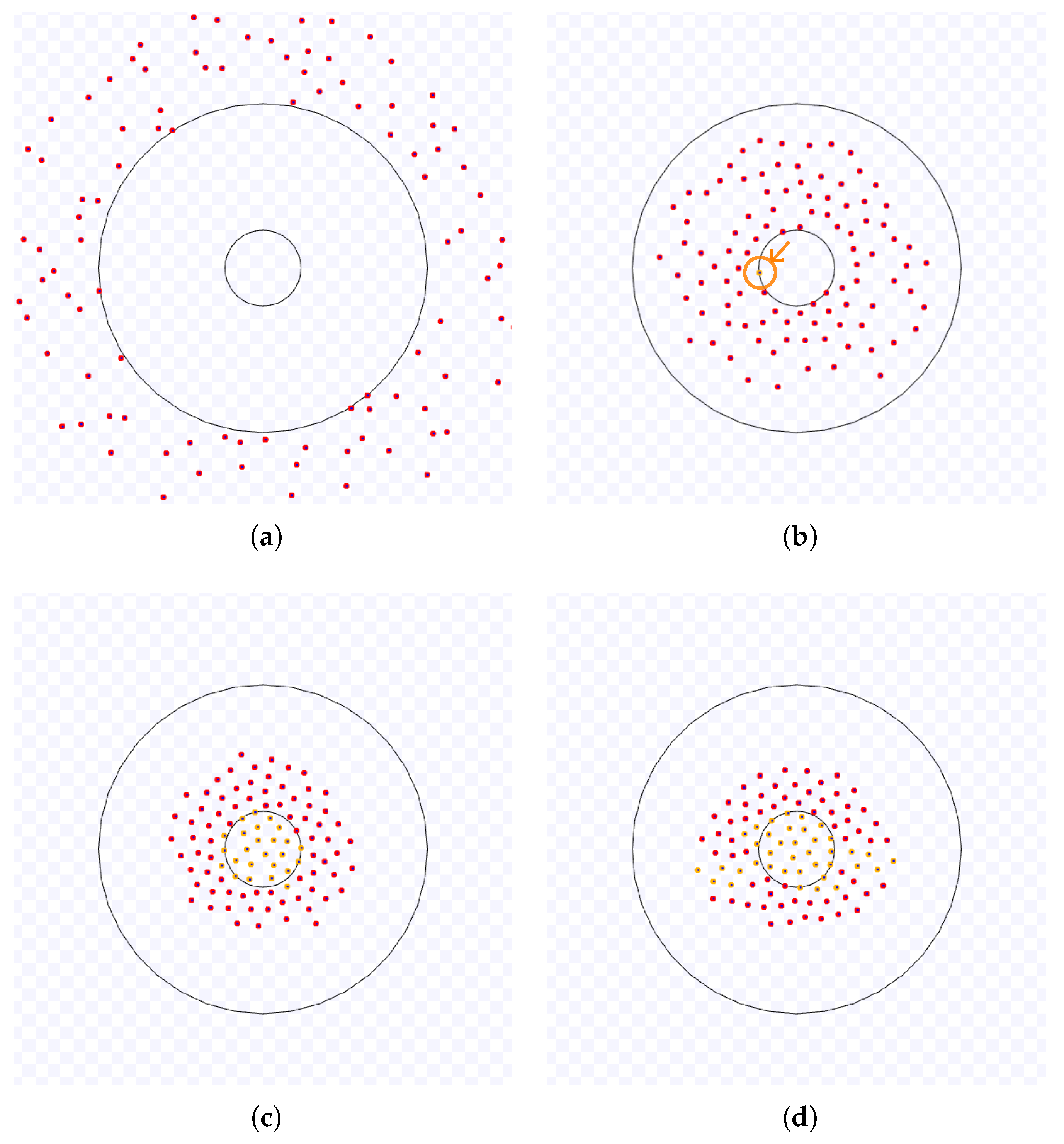
Figure 2.
Continuation of Figure 1. (e) Last queues near the end of the experiment. (f) The last robot to leave the working area.
Figure 2.
Continuation of Figure 1. (e) Last queues near the end of the experiment. (f) The last robot to leave the working area.
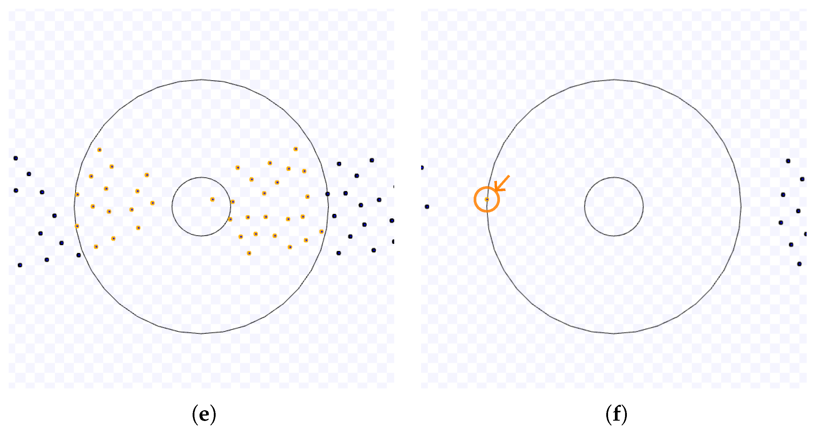
Figure 3.
Example of an experiment of the NC algorithm with and default values except for m. (a) Start of the experiment. (b) The first robot to reach the target area. (c) Free space in the middle of the target area. (d) A few robots going to the target area and more space inside the target area. Full simulation available on https://youtu.be/x0oO5DuAtwQ, accessed on 12 May 2023.
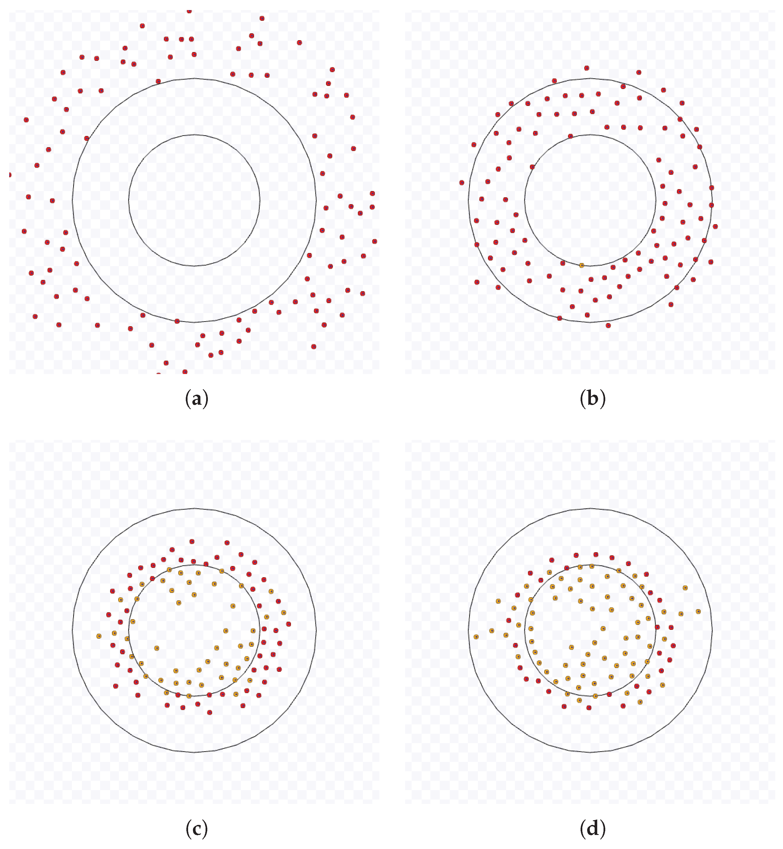
Figure 4.
Continuation of Figure 3. (e) Robots leave the target area with less resistance. (f) End of the experiment.
Figure 4.
Continuation of Figure 3. (e) Robots leave the target area with less resistance. (f) End of the experiment.
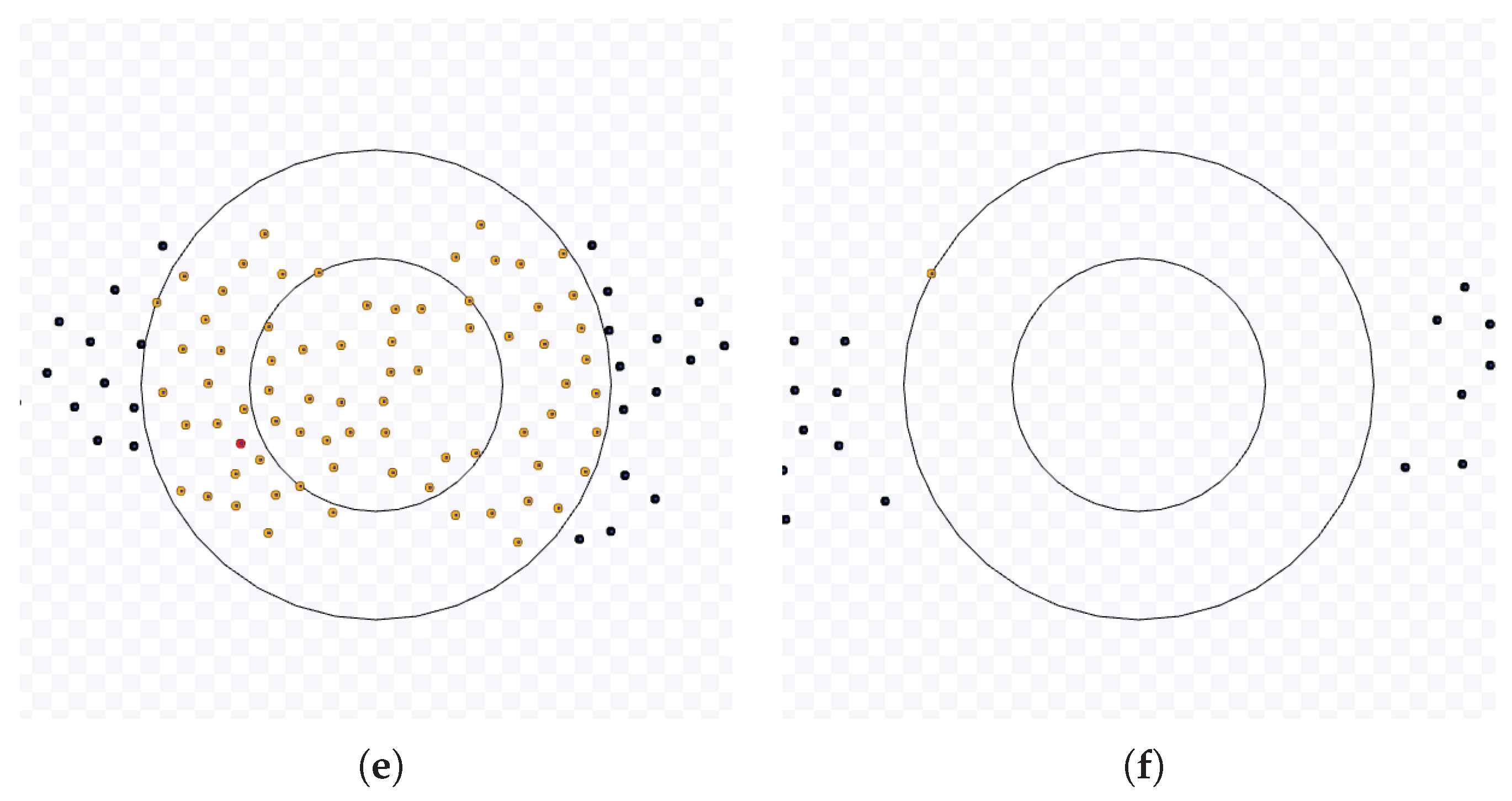
Figure 5.
Number of robots at a given time, , occupying a circle of radius r with robots distant by each other by . Red and yellow dots and circles represent robots going to and leaving the target area, respectively.
Figure 5.
Number of robots at a given time, , occupying a circle of radius r with robots distant by each other by . Red and yellow dots and circles represent robots going to and leaving the target area, respectively.
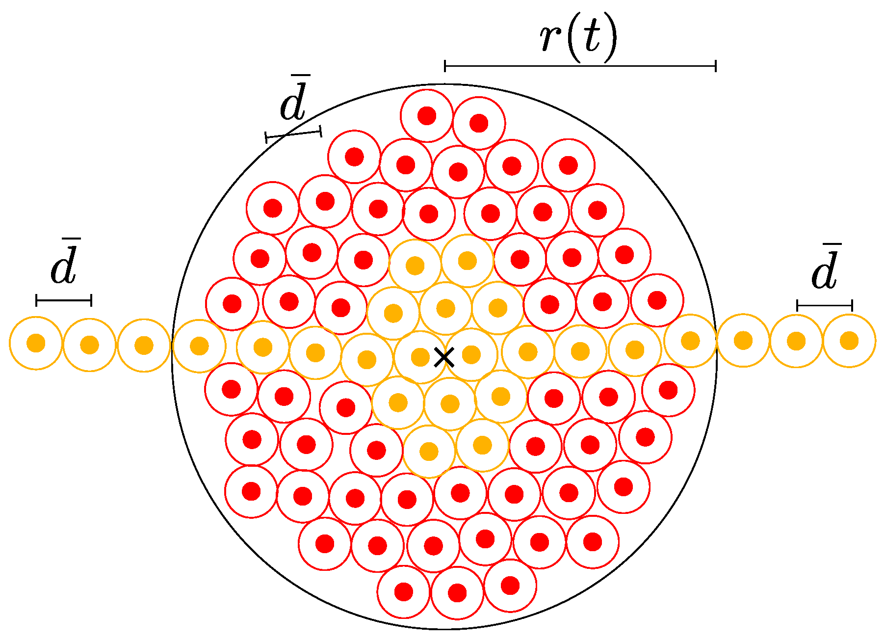
Figure 6.
(a) Rotational force field to reach the target with Single Queue Former algorithm [23]. (b) Rotational force field to leave the target in the SQF algorithm, and the distance from the central line of the corridor to the robot for varying its influence radius [23].
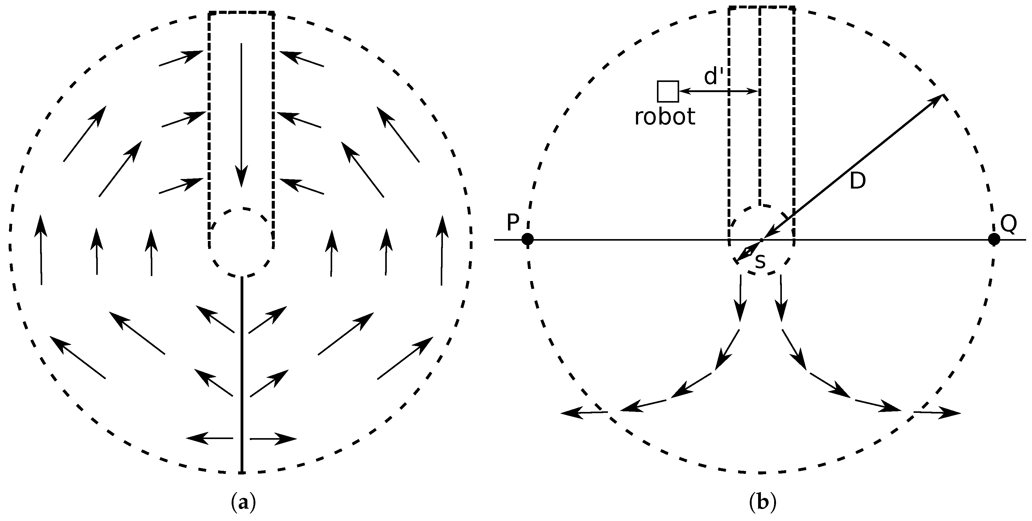
Figure 7.
Example of an experiment of the SQF algorithm with default values and . (a) Start of the experiment. (b) Bottom-most robot to reach the working area. (c) Robots waiting on both sides of the corridor. (d) The last robot to reach the corridor. Full simulation available on https://youtu.be/EdkCnUVw4Bg, accessed on 24 March 2023.
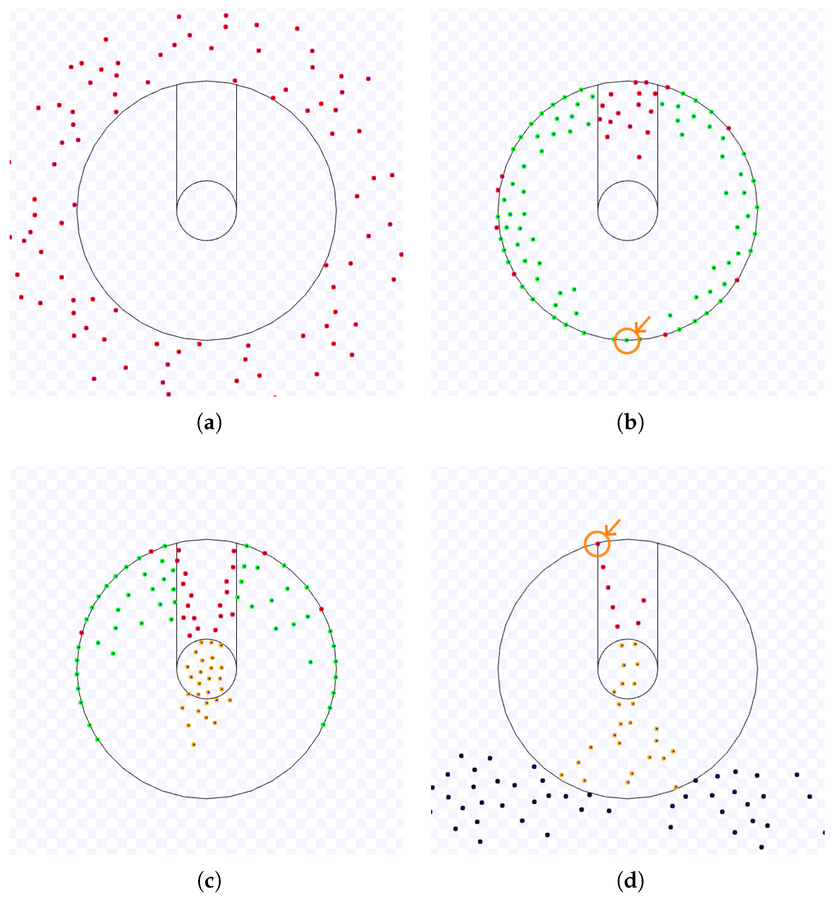
Figure 8.
Continuation of Figure 7. (e) The last robot to reach the target area. (f) The last robot to leave the working area.
Figure 8.
Continuation of Figure 7. (e) The last robot to reach the target area. (f) The last robot to leave the working area.
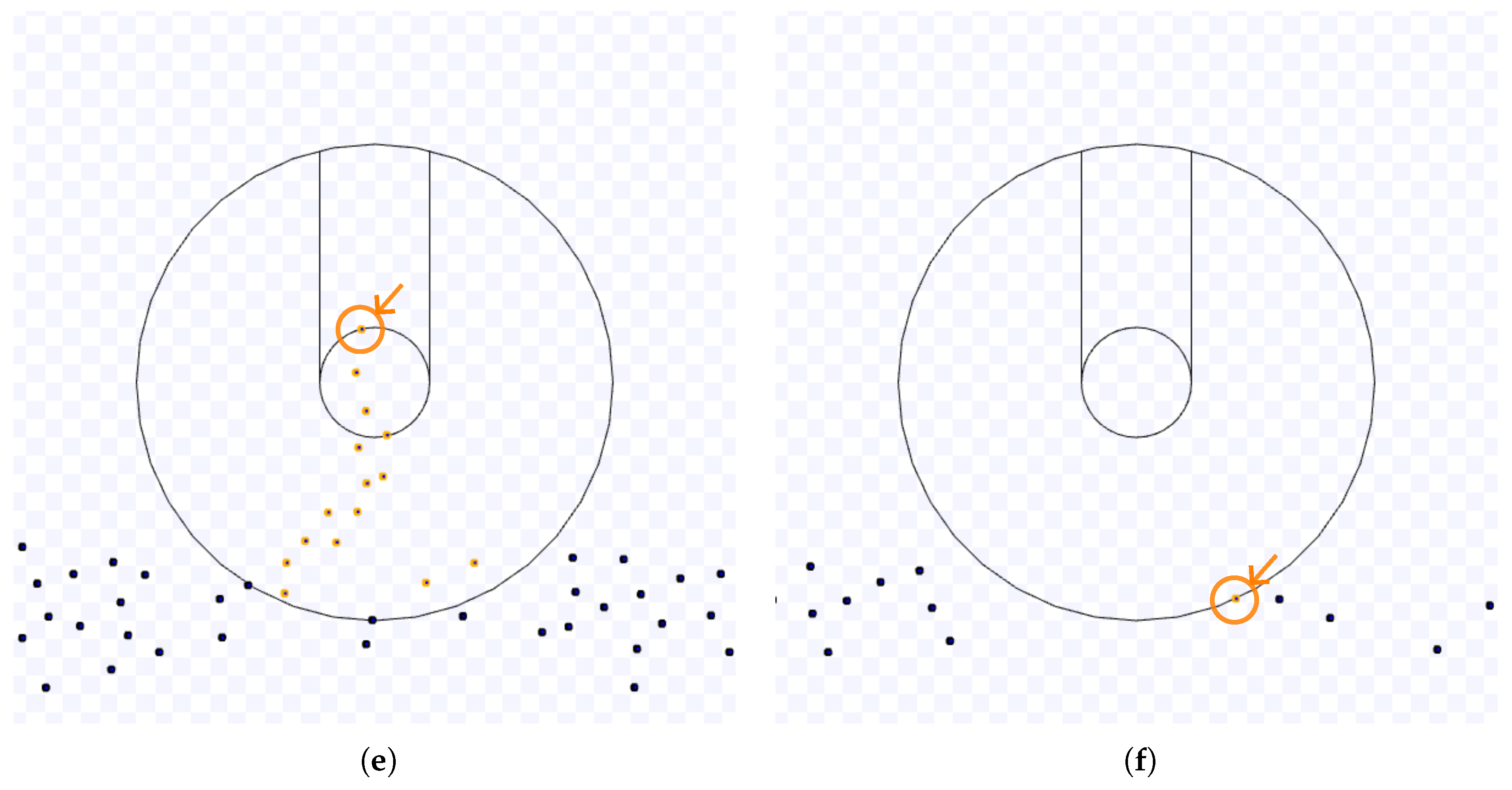
Figure 9.
Example of an experiment of the SQF algorithm with default values except for m and . (a) Start of the experiment. (b) The first robot to enter the target area by going to the corridor. (c) The first robot to leave the target area without passing through the corridor. (d) The first robot to leave the working area. Full simulation available on https://youtu.be/pEQzg0JwPbQ, accessed on 19 April 2023.
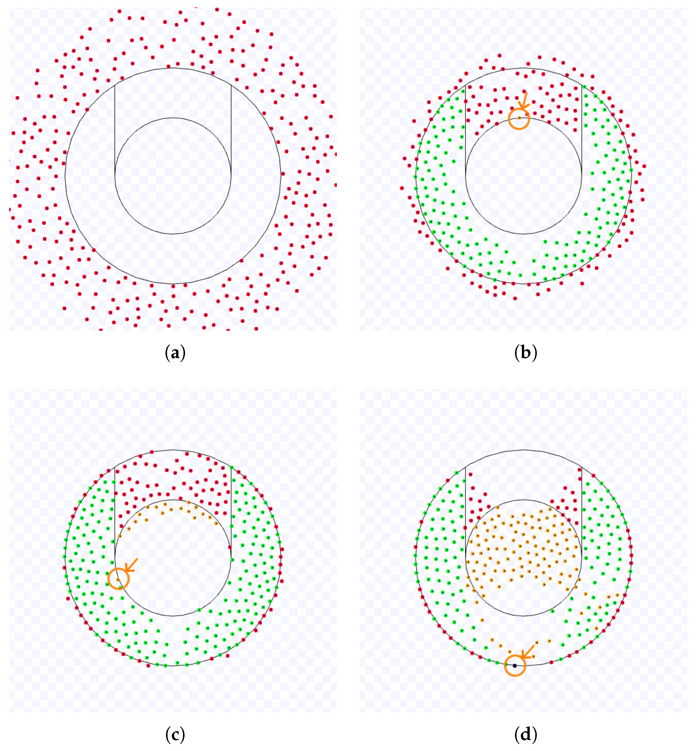
Figure 10.
Continuation of Figure 9. (e) Robots create a barrier obstructing others from leaving the working area. (f) The last robot to leave the working area.
Figure 10.
Continuation of Figure 9. (e) Robots create a barrier obstructing others from leaving the working area. (f) The last robot to leave the working area.
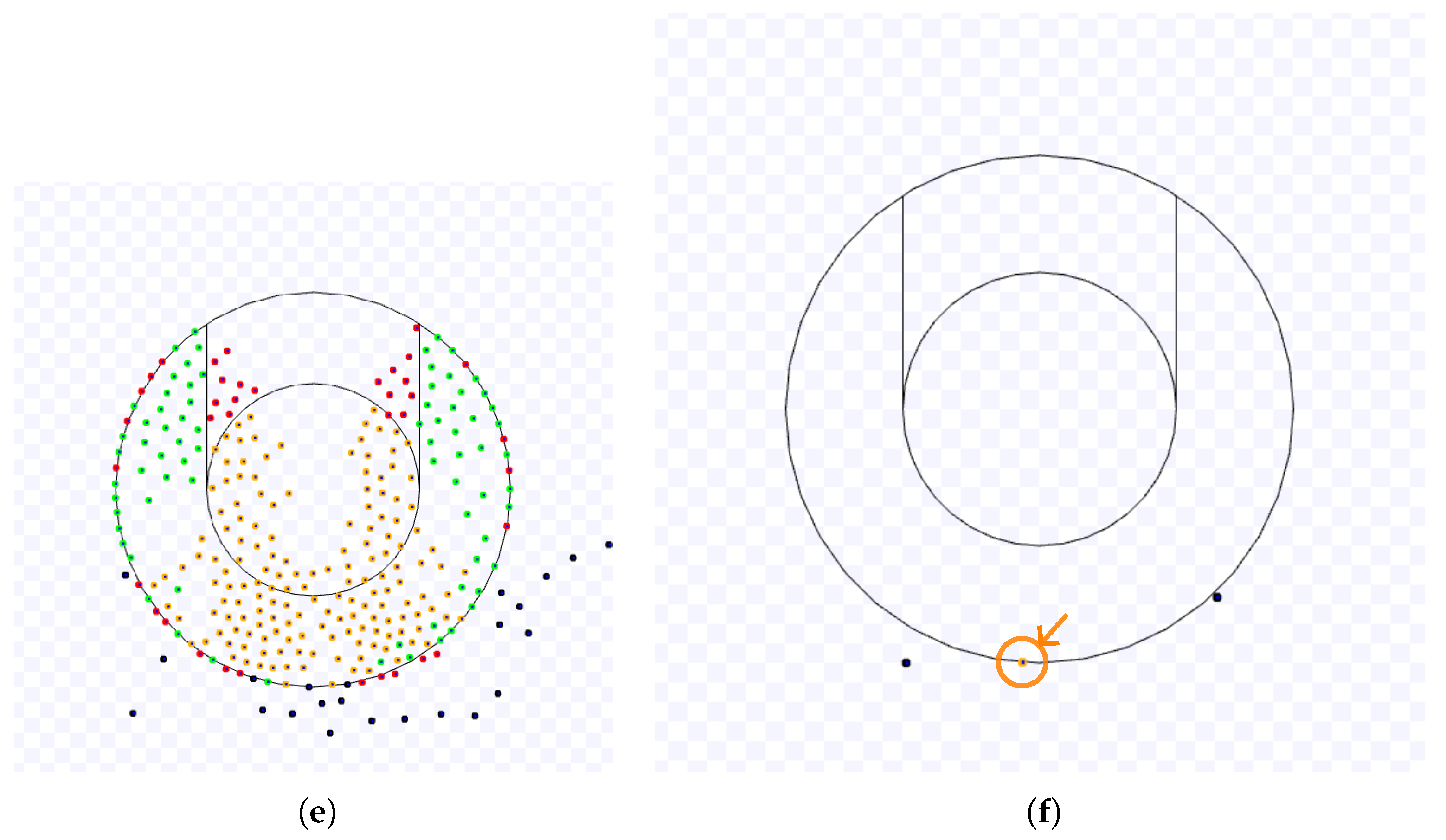
Figure 11.
(a) Dashed arc length from the expected target arriving location at to the working area border at . (b) Dashed arc length from the expected position of the bottom-most robot to the corridor corner . (c) Area considered for entry capacity for the SQF algorithm.
Figure 11.
(a) Dashed arc length from the expected target arriving location at to the working area border at . (b) Dashed arc length from the expected position of the bottom-most robot to the corridor corner . (c) Area considered for entry capacity for the SQF algorithm.
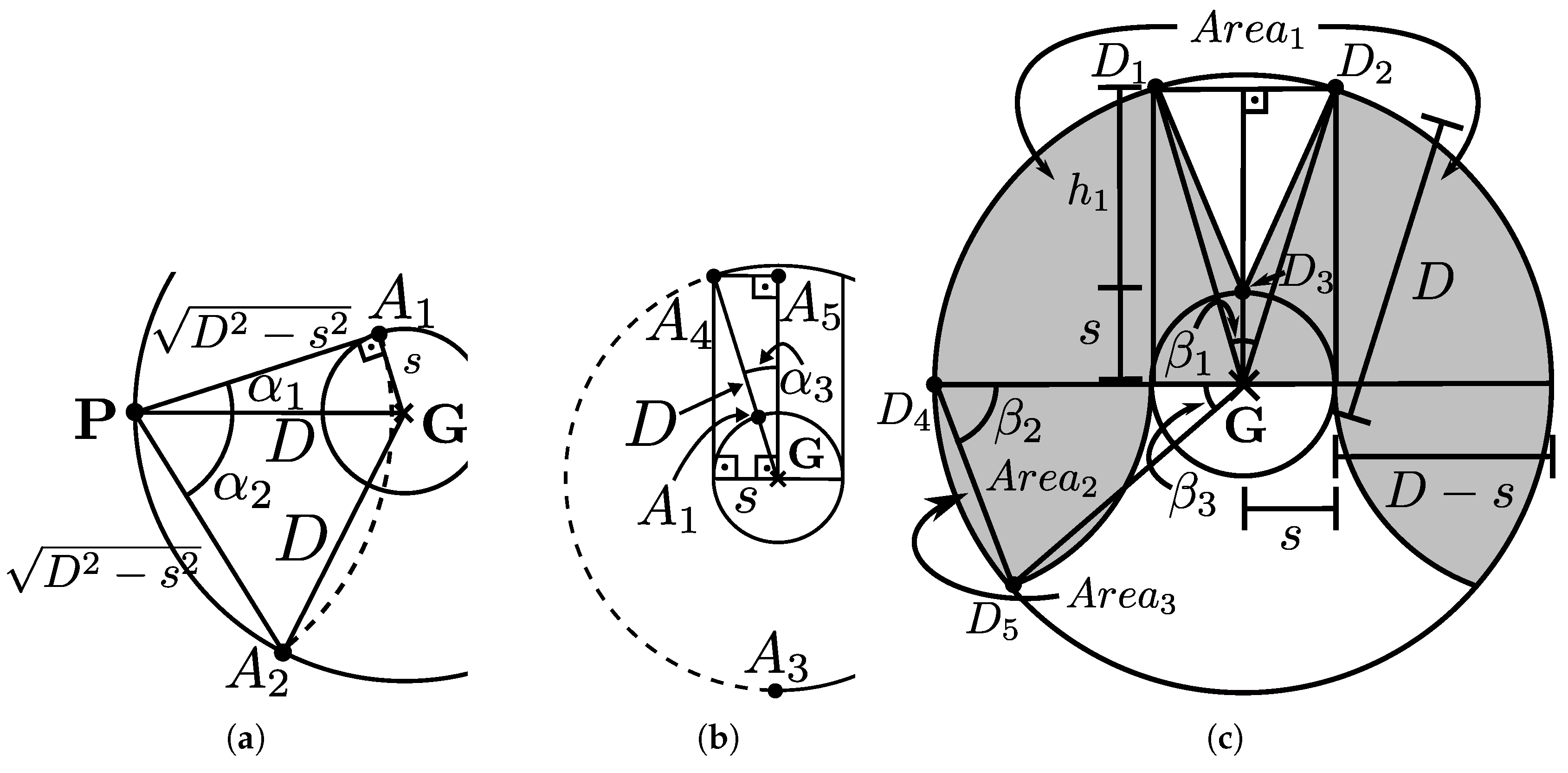
Figure 12.
Example of the lanes in TRVF algorithm with . The robots follow the waypoints , , and depending on the central angle region where they are located. The centre for the curved trajectory between waypoints and is distant by from the target centre .
Figure 12.
Example of the lanes in TRVF algorithm with . The robots follow the waypoints , , and depending on the central angle region where they are located. The centre for the curved trajectory between waypoints and is distant by from the target centre .
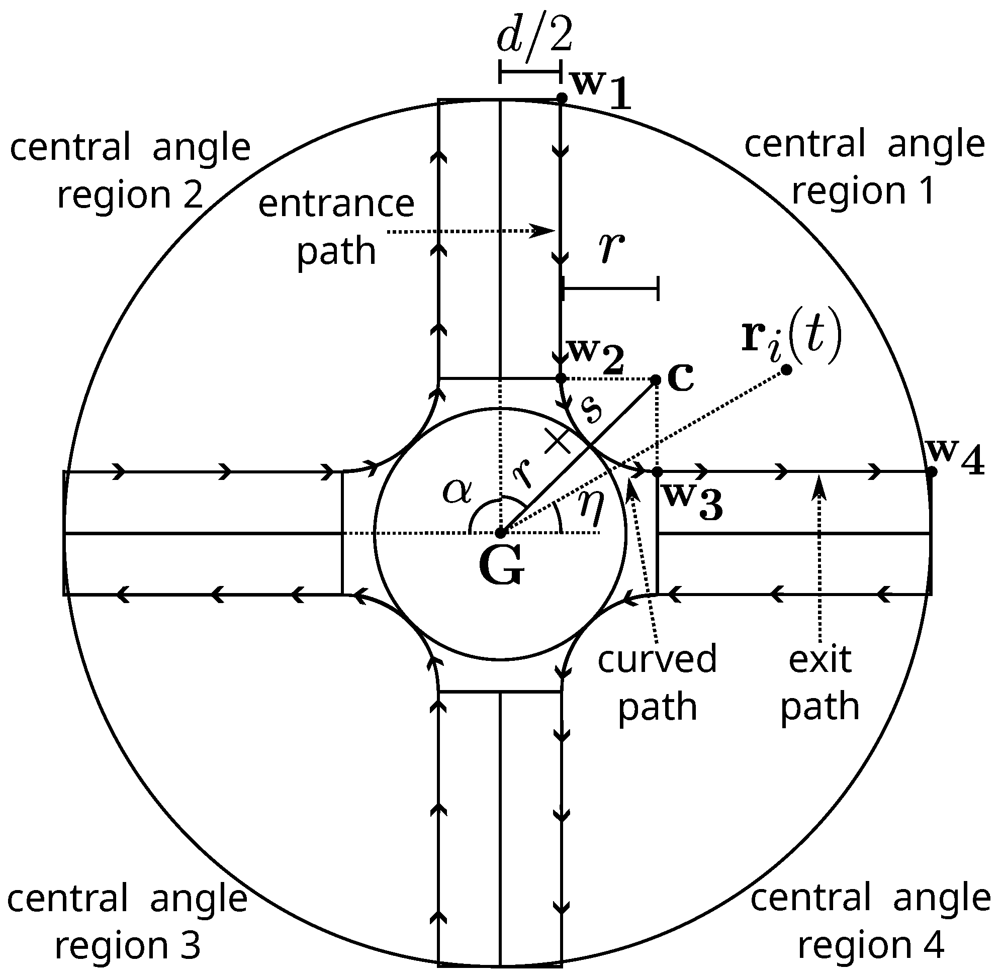
Figure 13.
Example of an experiment of the TRVF algorithm with default values and . (a) Start of the experiment. (b) Robots go through the entrance path. (c) The first robot to reach the target area. (d) The first robot to leave the working area. Full simulation available on https://youtu.be/bNIgvgpl_J4, accessed on 14 October 2022.
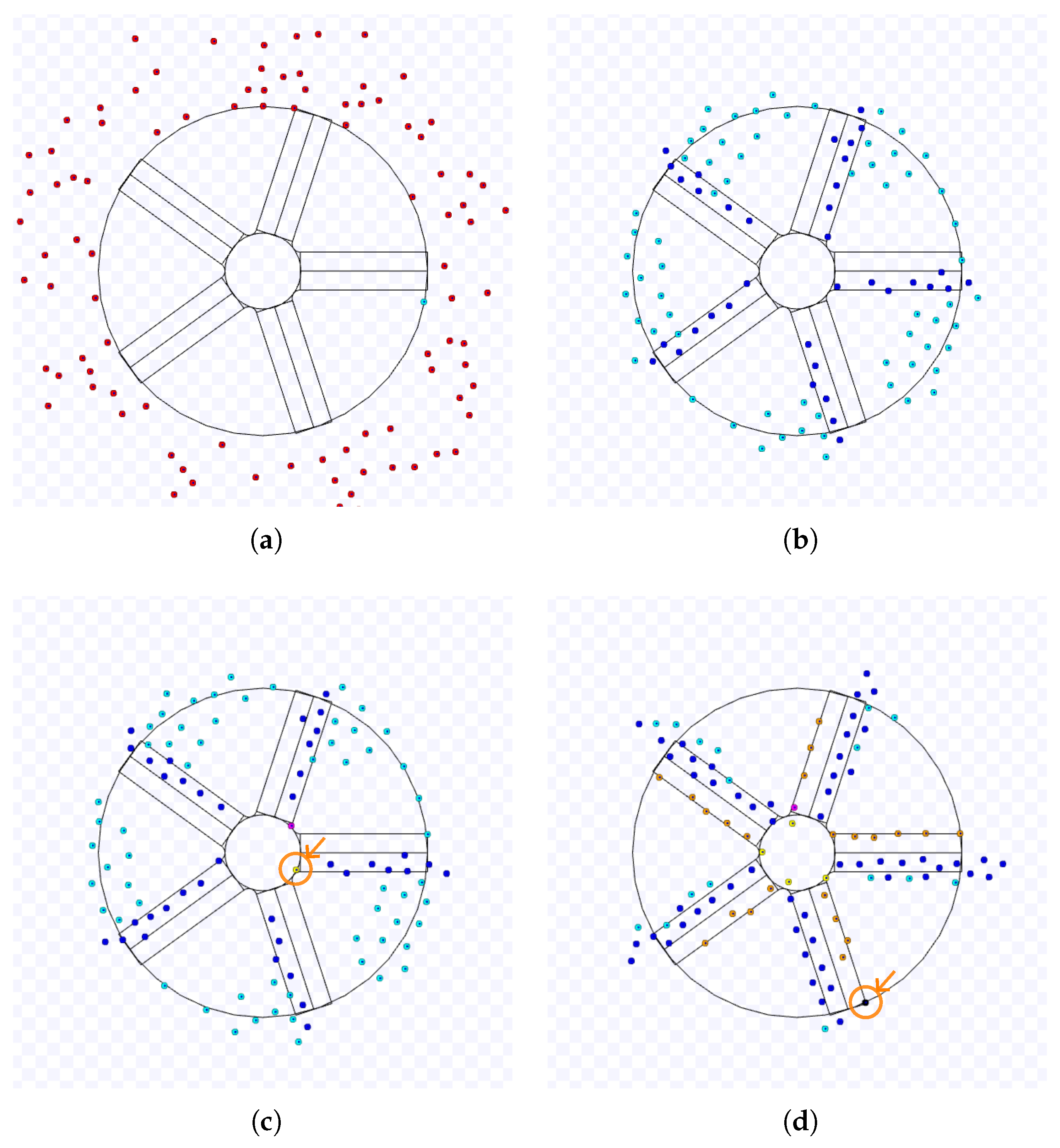
Figure 14.
Continuation of Figure 13. (e) The last robot to reach the target area. (f) End of the experiment.
Figure 14.
Continuation of Figure 13. (e) The last robot to reach the target area. (f) End of the experiment.
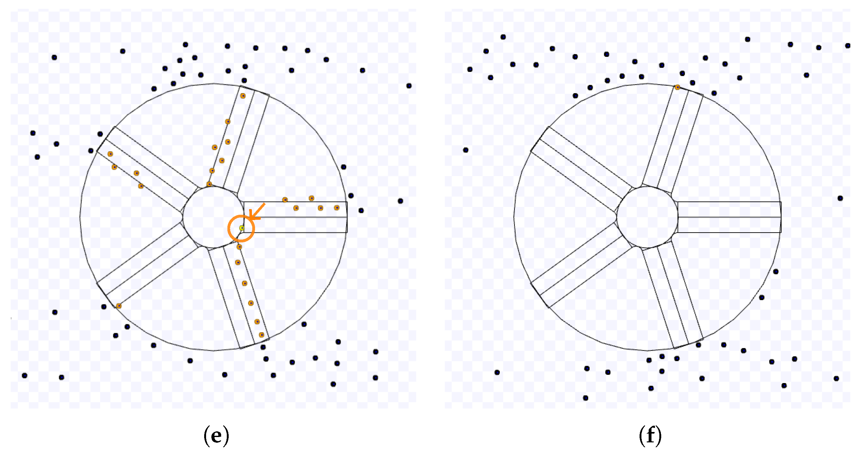
Figure 15.
(a) Sector angle where the first robot on that lane arrives. (b) Estimated location where the first robot will arrive at the target area. (c) Right triangles and for calculating the lenghts and .
Figure 15.
(a) Sector angle where the first robot on that lane arrives. (b) Estimated location where the first robot will arrive at the target area. (c) Right triangles and for calculating the lenghts and .
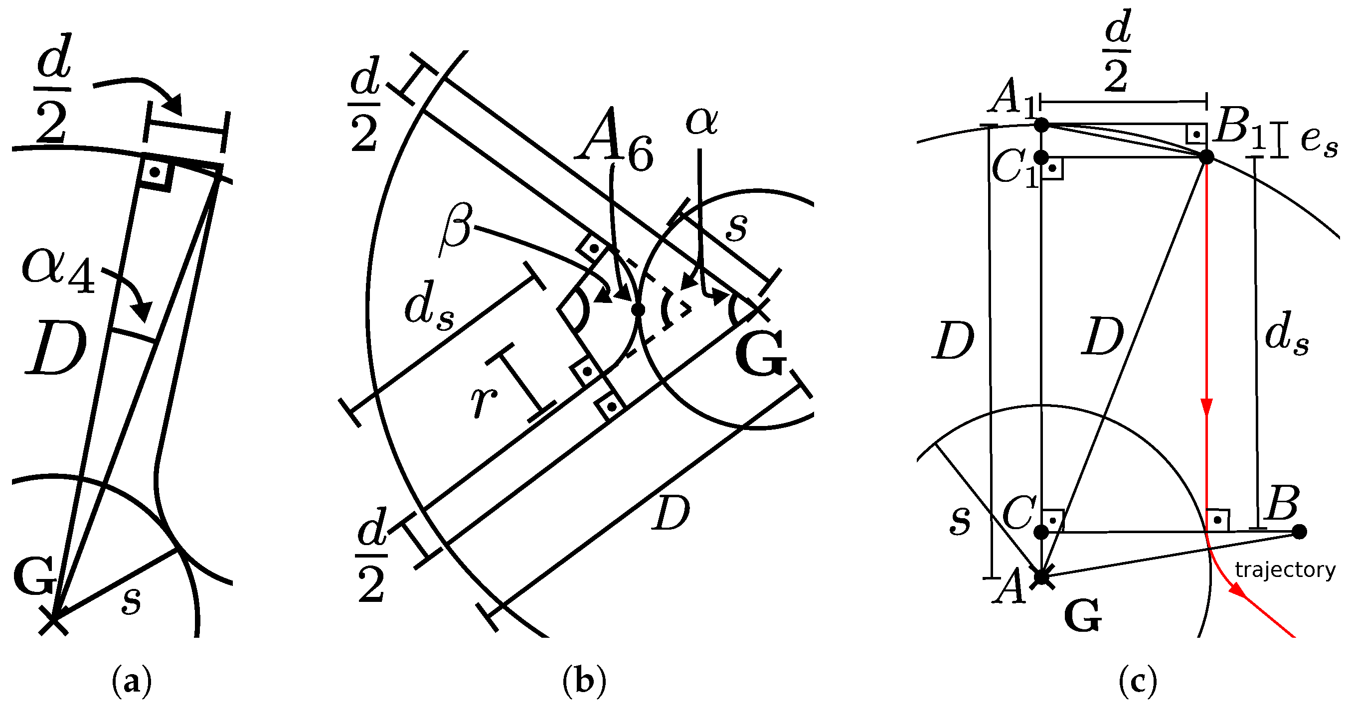
Figure 16.
Example of an experiment of MT with 10% of robots in group A ( and ) and the SQF algorithm executed by group B. (a) Start of the experiment. (b) Robots using NC go directly to the target. (c) Some grey robots go to the next target. (d) The last robots using NC leave the target, but SQF robots are on their way to the next target. Full simulation available on https://youtu.be/uBetIxGOl20, accessed on 24 April 2023.
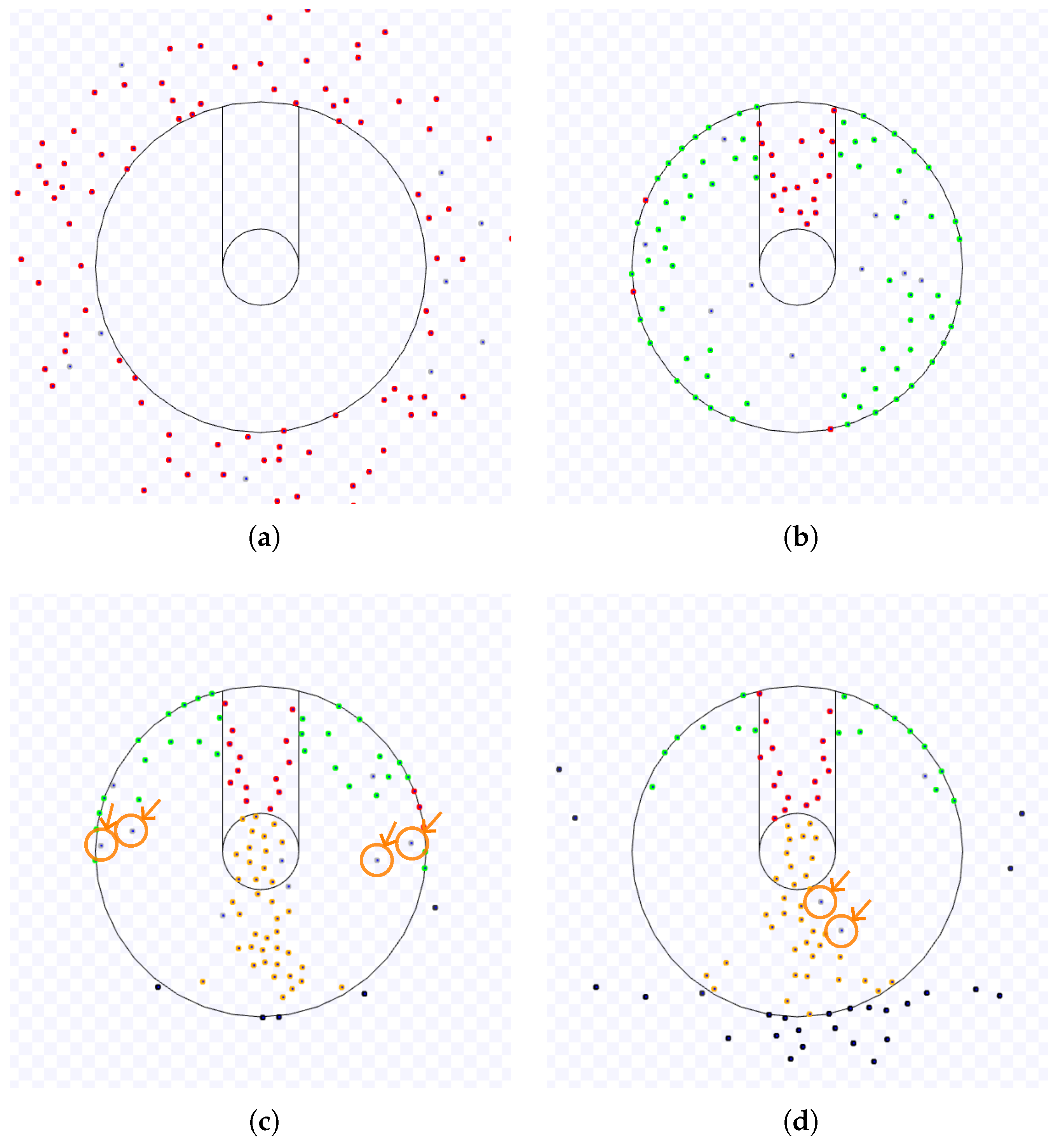
Figure 17.
Continuation of Figure 16. (e) The last grey robots leave the working area through the SQF-induced leaving route. (f) The remaining robots use the SQF algorithm near the end.
Figure 17.
Continuation of Figure 16. (e) The last grey robots leave the working area through the SQF-induced leaving route. (f) The remaining robots use the SQF algorithm near the end.
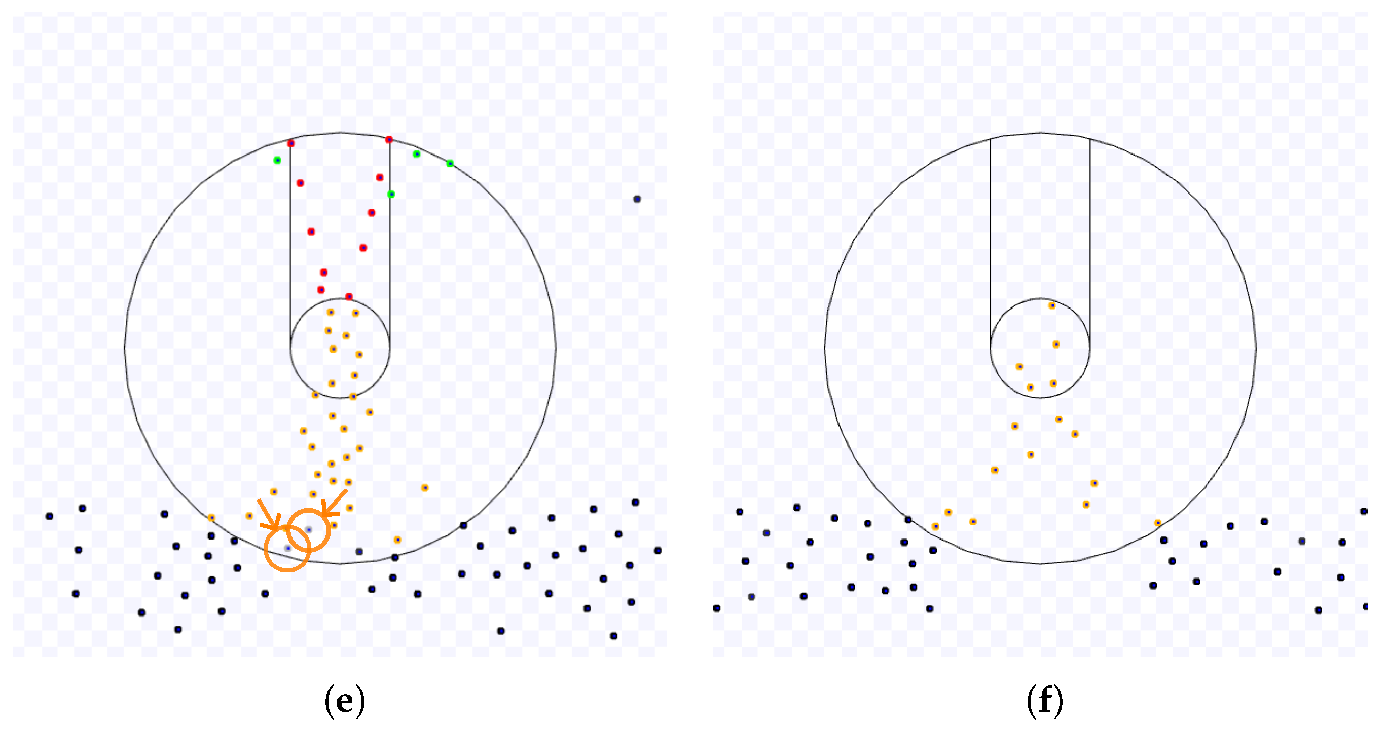
Figure 18.
Example of an experiment of MT with 50% of robots in group A ( and ) and the SQF algorithm executed by group B. (a) Start of the experiment. (b) Robots using NC go directly to the target. (c) Robots using NC go to the target after being pushed by SQF robots leaving the target. (d) The last robot using SQF reaches the target area. Full simulation available on https://youtu.be/a-05slaNud8, accessed on 24 April 2023.
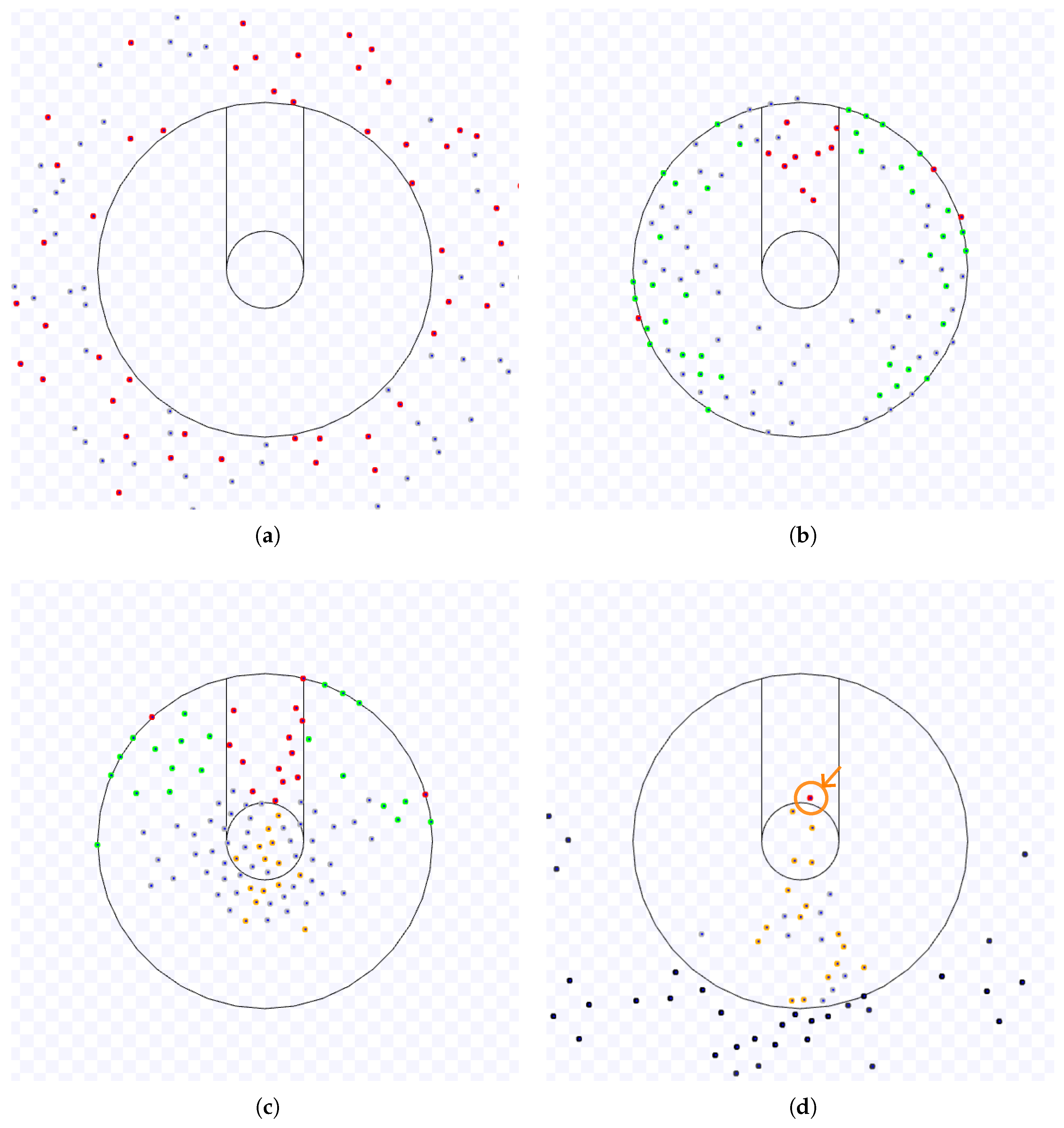
Figure 19.
Continuation of Figure 18. (e) The robots on the SQF-induced leaving route are the last to arrive at the target region. (f) End of the experiment.
Figure 19.
Continuation of Figure 18. (e) The robots on the SQF-induced leaving route are the last to arrive at the target region. (f) End of the experiment.
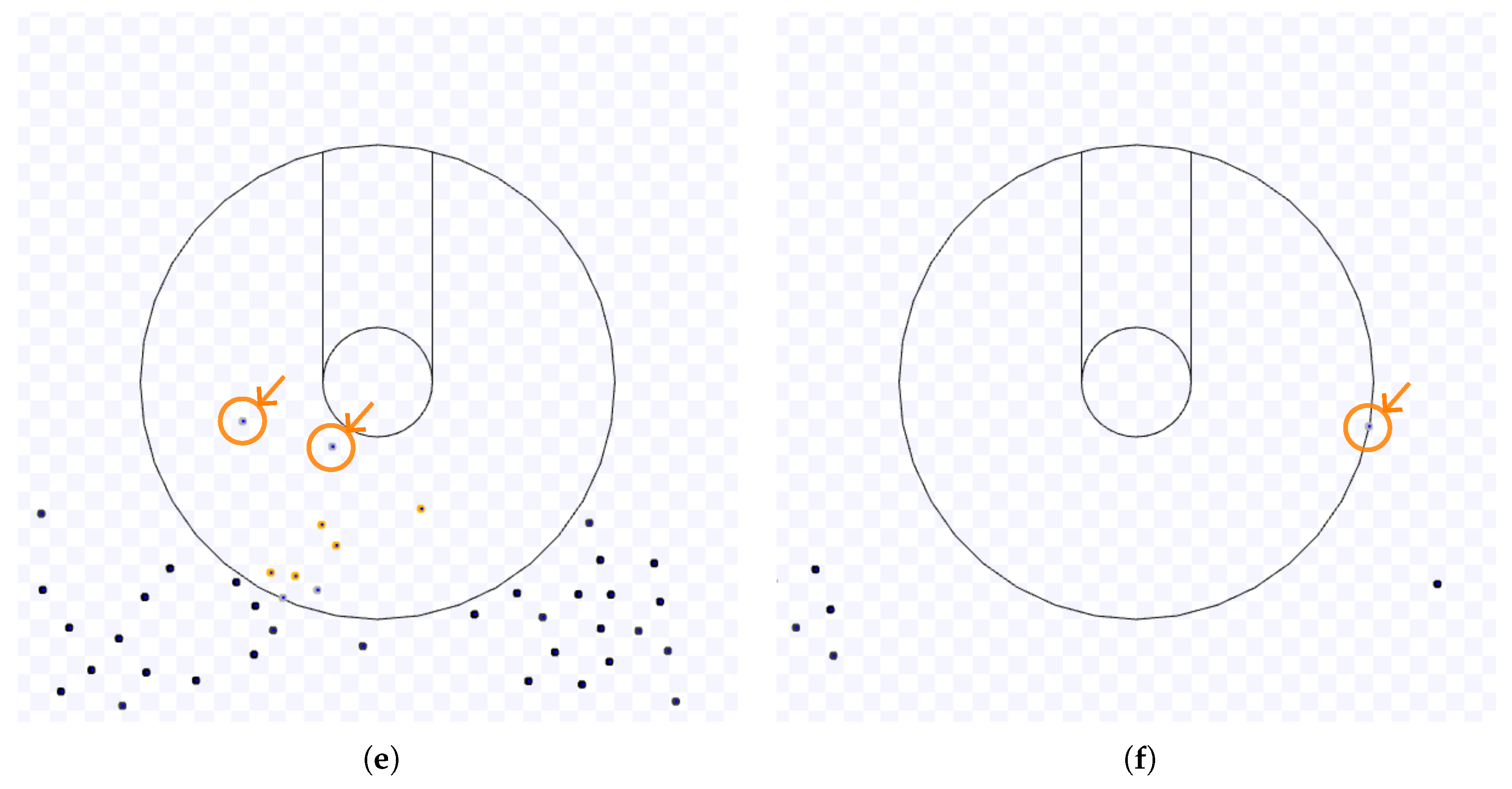
Figure 20.
Example of an experiment of MT with 10% of robots in group A ( and ) and the TRVF algorithm executed by group B. (a) Start of the experiment. (b) Robots using NC arrive at the target area through the free space. (c) A grey robot using NC waits for robots in a lane. (d) The last grey robot is leaving the working area. Full simulation available on https://youtu.be/VlhXKM77q90, accessed on 24 April 2023.
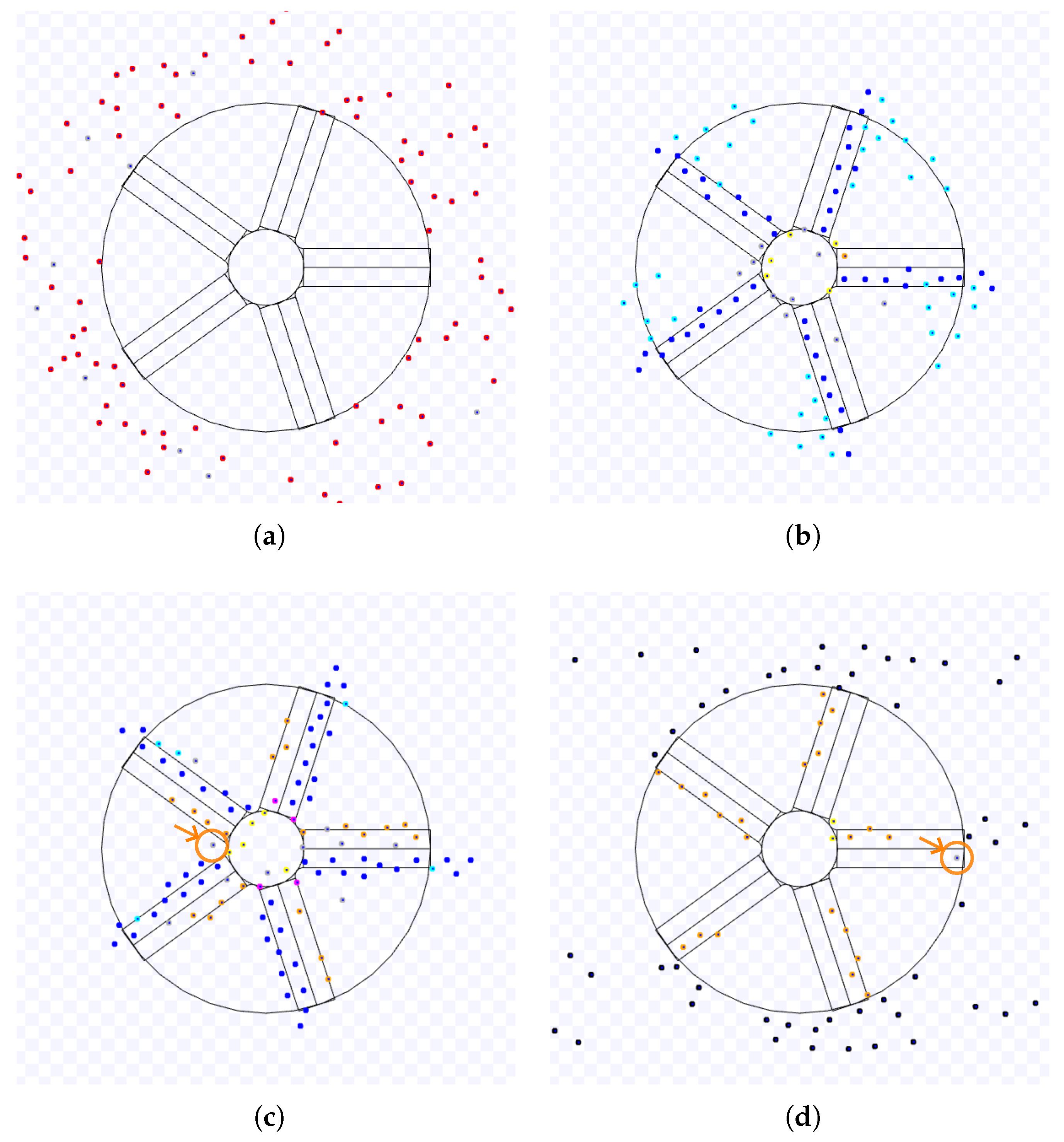
Figure 21.
Continuation of Figure 20. (e) Only robots using TRVF are inside the working area. (f) End of the experiment.
Figure 21.
Continuation of Figure 20. (e) Only robots using TRVF are inside the working area. (f) End of the experiment.
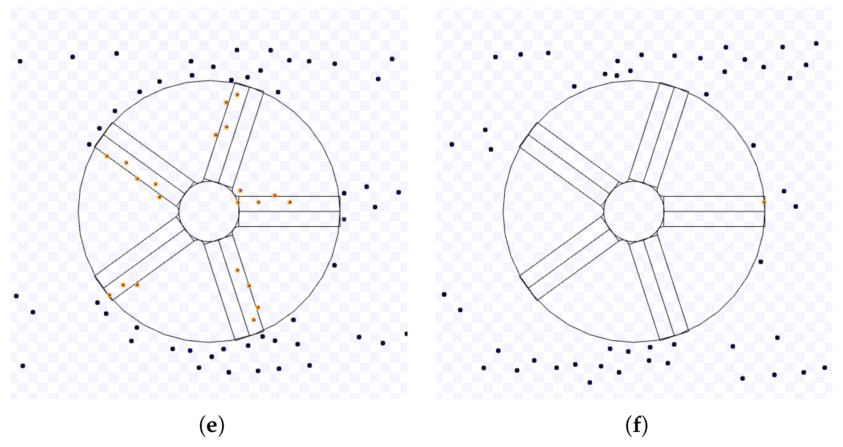
Figure 22.
Example of an experiment of MT with 50% of robots in group A ( and ) and the TRVF algorithm executed by group B. (a) Start of the experiment. (b) Robots using NC go directly to the target. (c) NC robots (in grey) cluster in the target area. (d) NC robots interfere with the access of robots using TRVF. Full simulation available on https://youtu.be/1nxSEsre5mk, accessed on 24 April 2023.
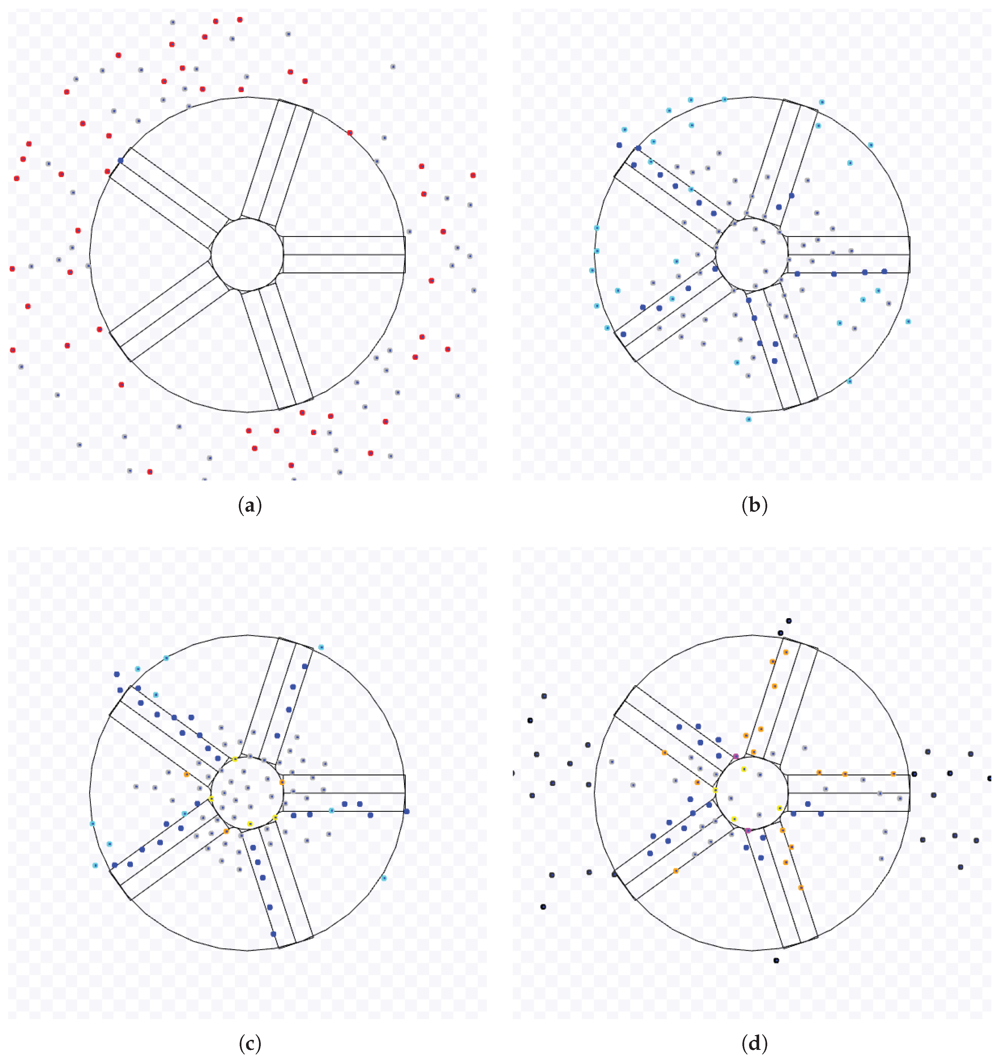
Figure 23.
Continuation of Figure 22. (e) The last robot using NC leaves the working area. (f) End of the experiment.
Figure 23.
Continuation of Figure 22. (e) The last robot using NC leaves the working area. (f) End of the experiment.
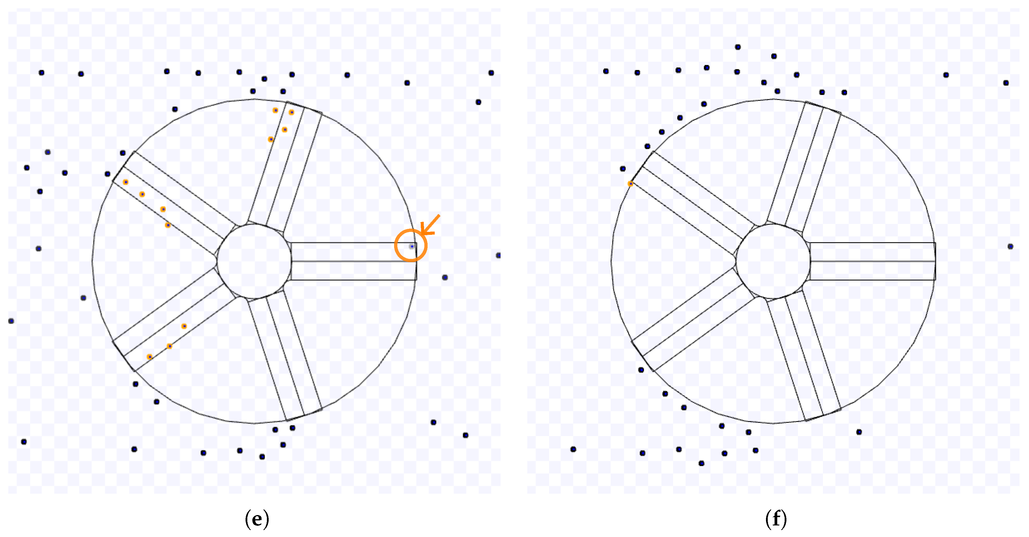
Figure 24.
Task completion time versus the number of robots for NC, SQF and an MT with NC as the group A algorithm and robots in group B with SQF for holonomic robots and (a) , (b) and (c) .
Figure 24.
Task completion time versus the number of robots for NC, SQF and an MT with NC as the group A algorithm and robots in group B with SQF for holonomic robots and (a) , (b) and (c) .
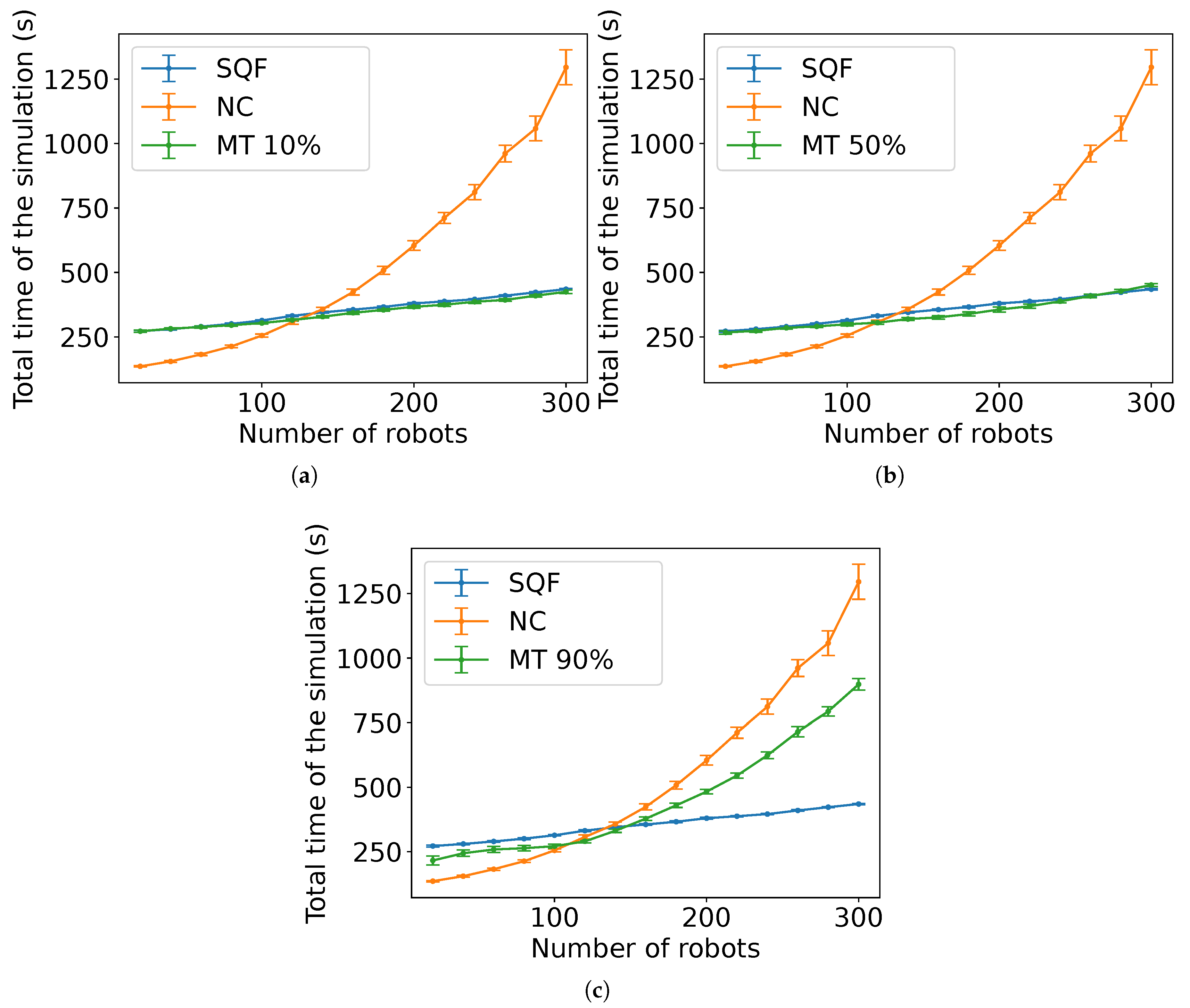
Figure 25.
Task completion time versus the number of robots for NC, TRVF and MT with NC as the group A algorithm and robots in group B with TRVF for holonomic robots and (a) , (b) and (c) .
Figure 25.
Task completion time versus the number of robots for NC, TRVF and MT with NC as the group A algorithm and robots in group B with TRVF for holonomic robots and (a) , (b) and (c) .
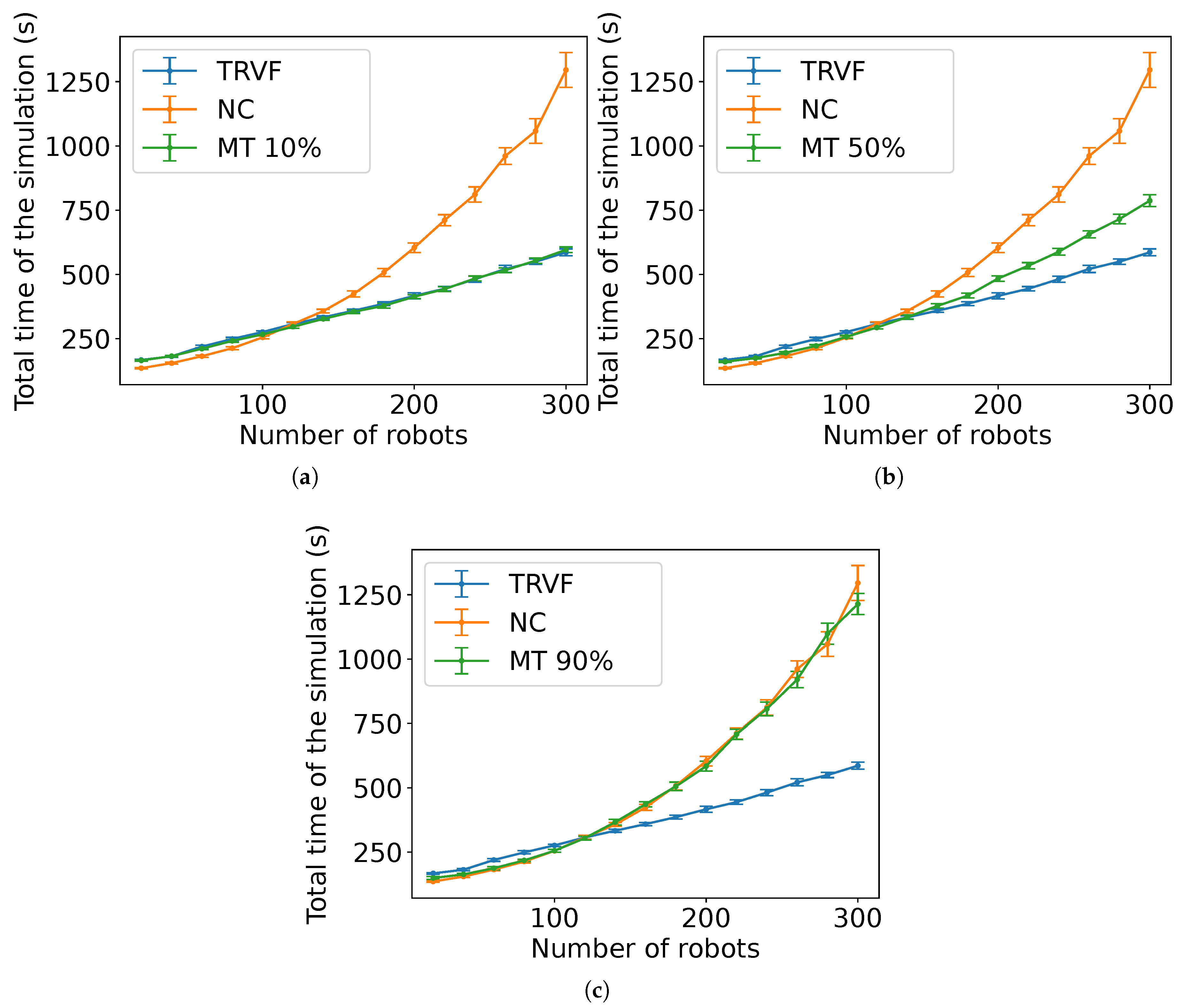
Figure 26.
Comparison of the estimated expected time and the experimental data for NC, m with (a) holonomic robots () and (b) non-holonomic robots () and m with (a) holonomic robots () and (b) non-holonomic robots ().
Figure 26.
Comparison of the estimated expected time and the experimental data for NC, m with (a) holonomic robots () and (b) non-holonomic robots () and m with (a) holonomic robots () and (b) non-holonomic robots ().
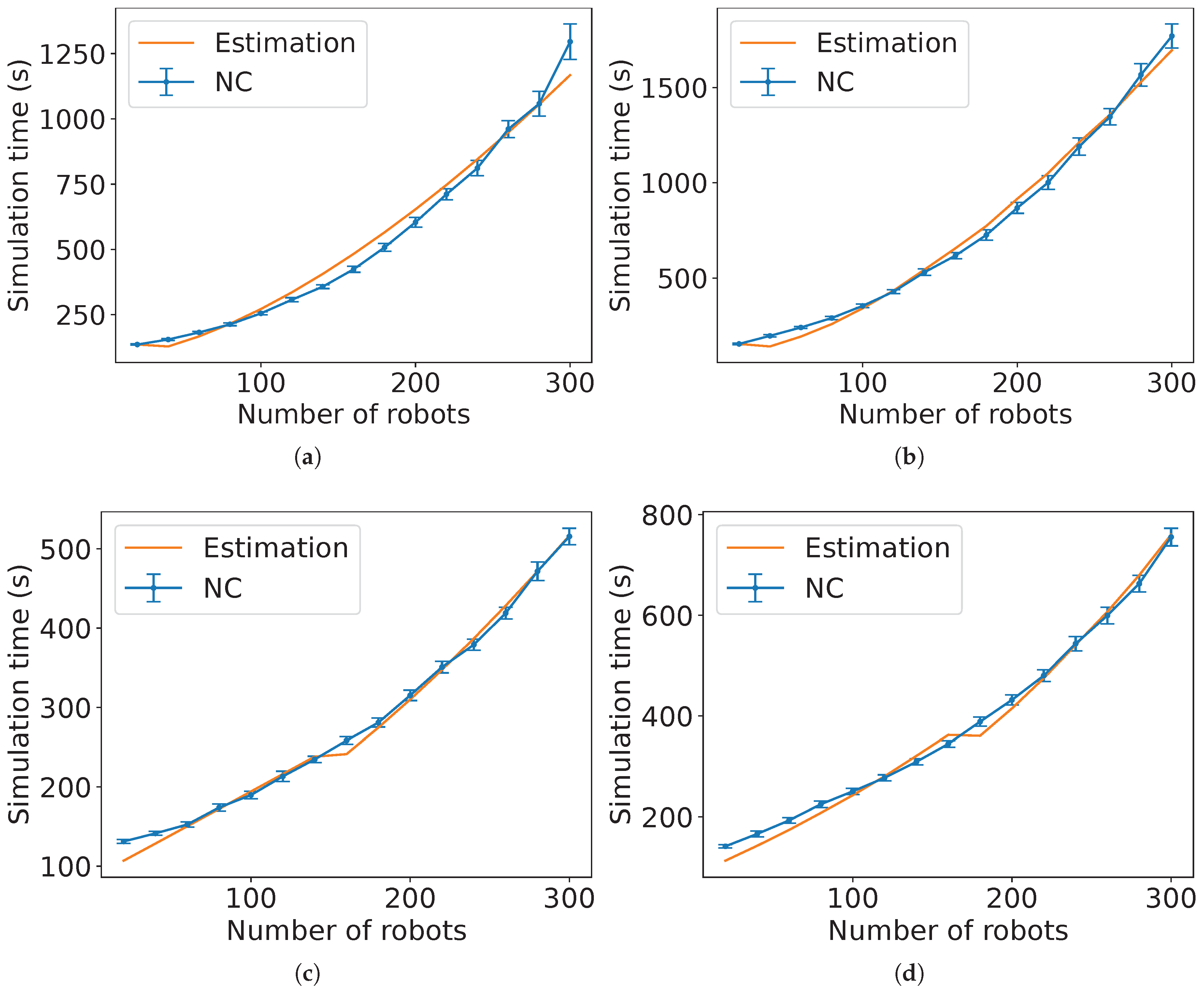
Figure 27.
Comparison of the estimated expected time and the experimental data for NC, m with (a) holonomic robots () and (b) non-holonomic robots ().
Figure 27.
Comparison of the estimated expected time and the experimental data for NC, m with (a) holonomic robots () and (b) non-holonomic robots ().
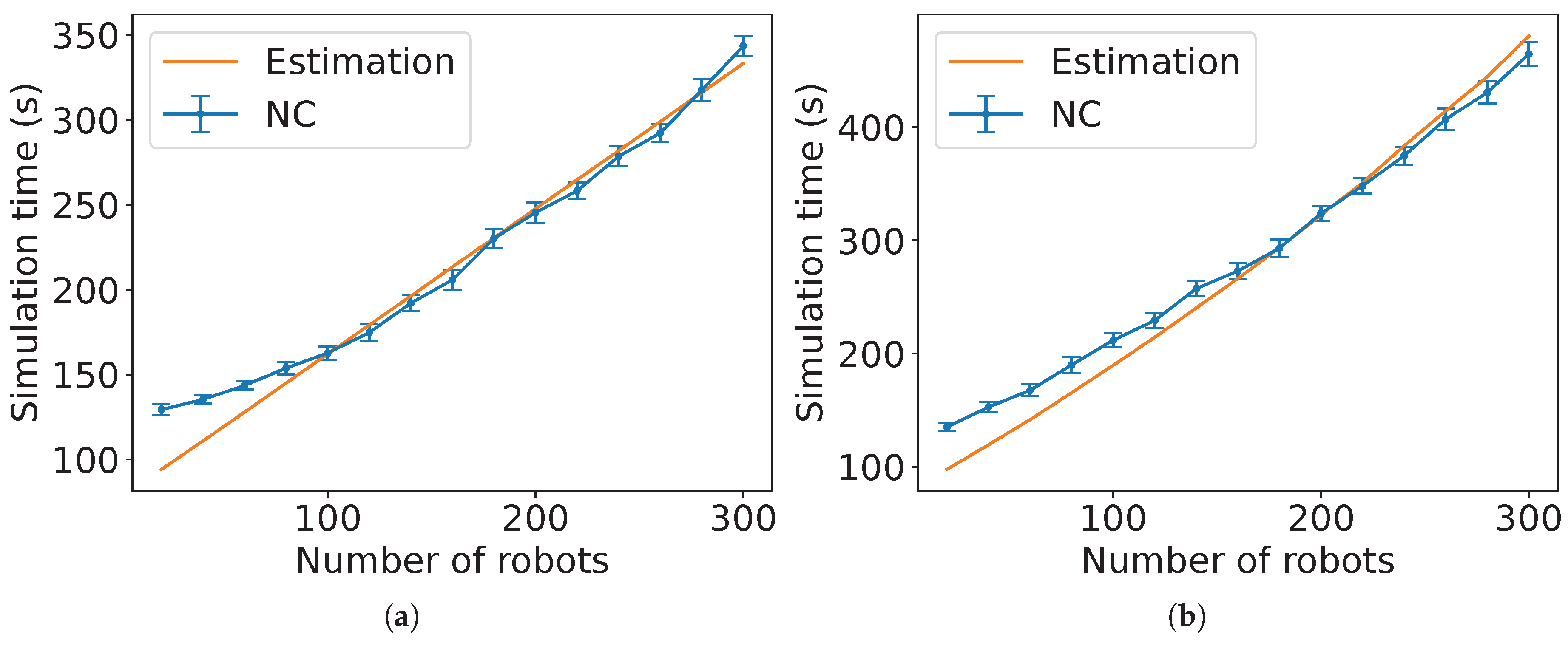
Figure 28.
Comparison of the estimated expected time and the experimental data for the SQF algorithm, m with (a) holonomic robots () and (b) non-holonomic robots () and m with (c) holonomic robots () and (d) non-holonomic robots ().
Figure 28.
Comparison of the estimated expected time and the experimental data for the SQF algorithm, m with (a) holonomic robots () and (b) non-holonomic robots () and m with (c) holonomic robots () and (d) non-holonomic robots ().
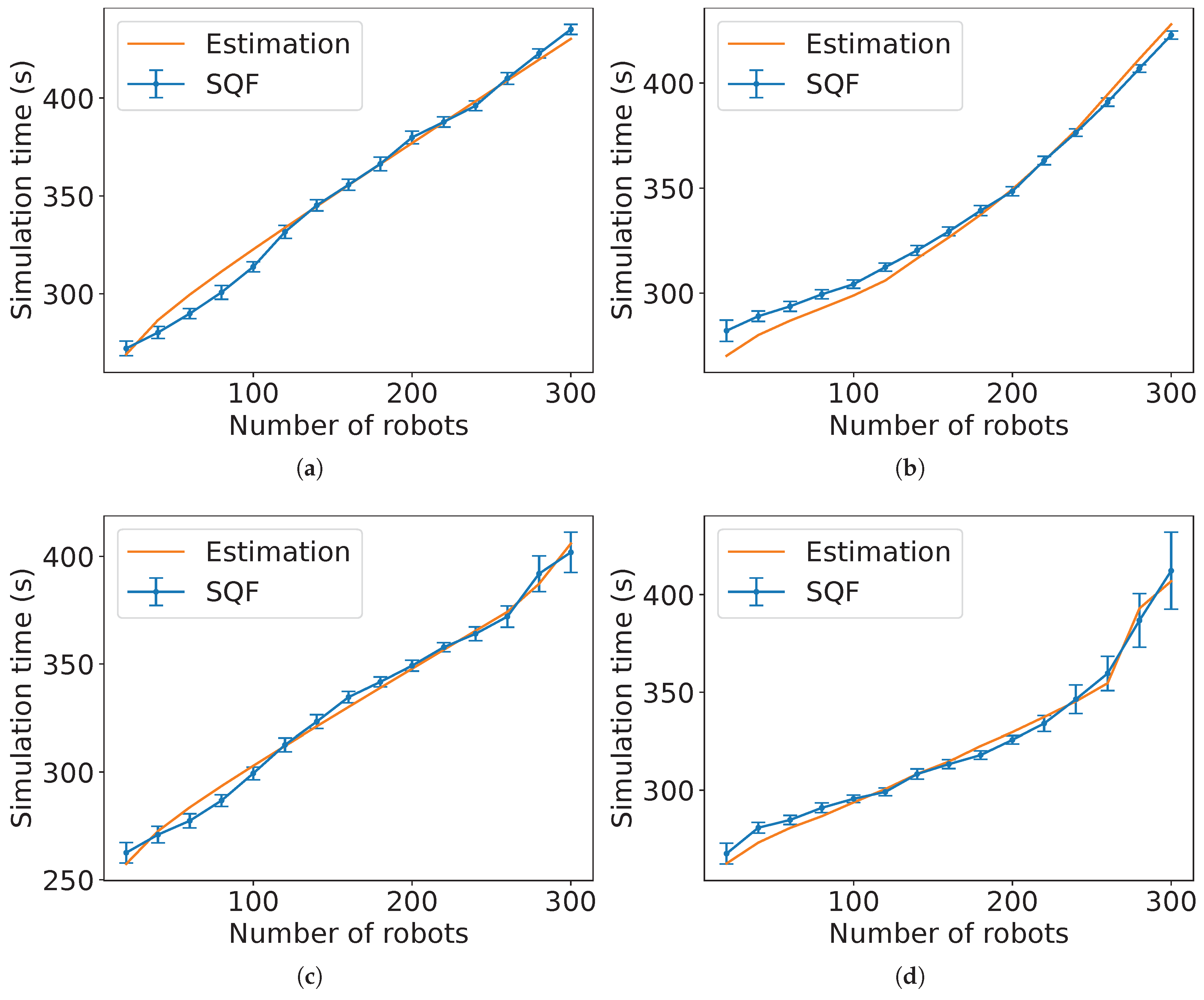
Figure 29.
Comparison of the estimated expected time and the experimental data for the SQF algorithm, m with (a) holonomic robots () and (b) non-holonomic robots ().
Figure 29.
Comparison of the estimated expected time and the experimental data for the SQF algorithm, m with (a) holonomic robots () and (b) non-holonomic robots ().
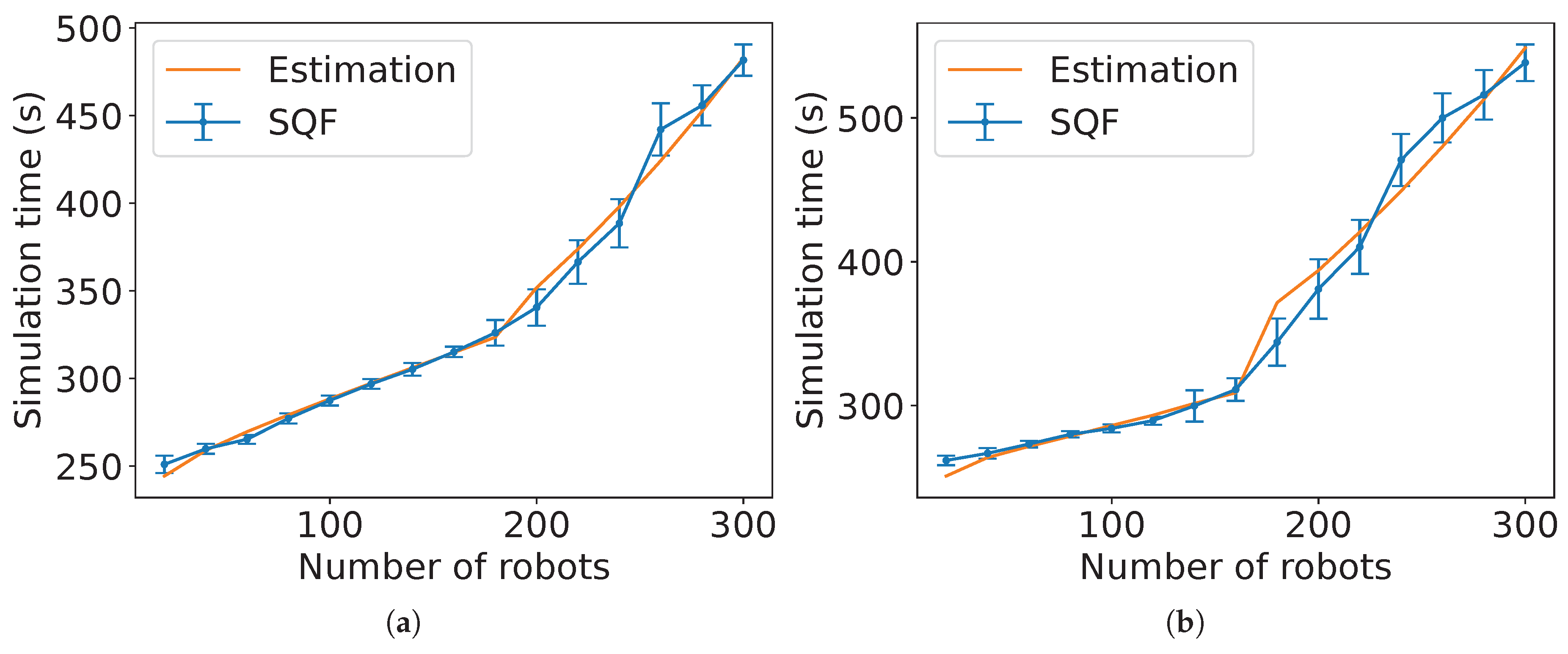
Figure 30.
Comparison of the estimated expected time and the experimental data for the TRVF algorithm, m with (a) holonomic robots () and (b) non-holonomic robots () and m with (c) holonomic robots () and (d) non-holonomic robots ().
Figure 30.
Comparison of the estimated expected time and the experimental data for the TRVF algorithm, m with (a) holonomic robots () and (b) non-holonomic robots () and m with (c) holonomic robots () and (d) non-holonomic robots ().
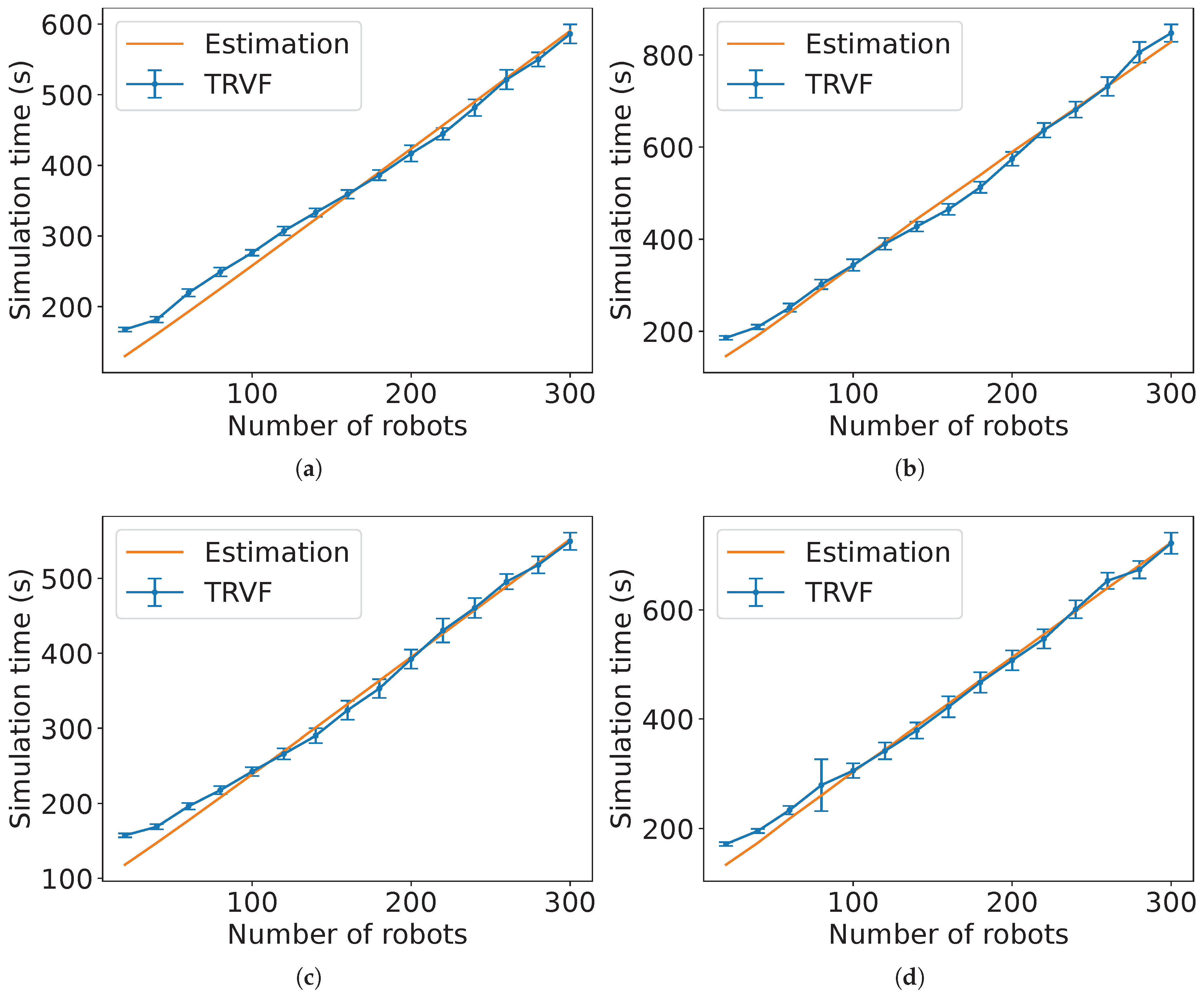
Figure 31.
Comparison of the estimated expected time and the experimental data for the TRVF algorithm, m with (a) holonomic robots () and (b) non-holonomic robots ().
Figure 31.
Comparison of the estimated expected time and the experimental data for the TRVF algorithm, m with (a) holonomic robots () and (b) non-holonomic robots ().
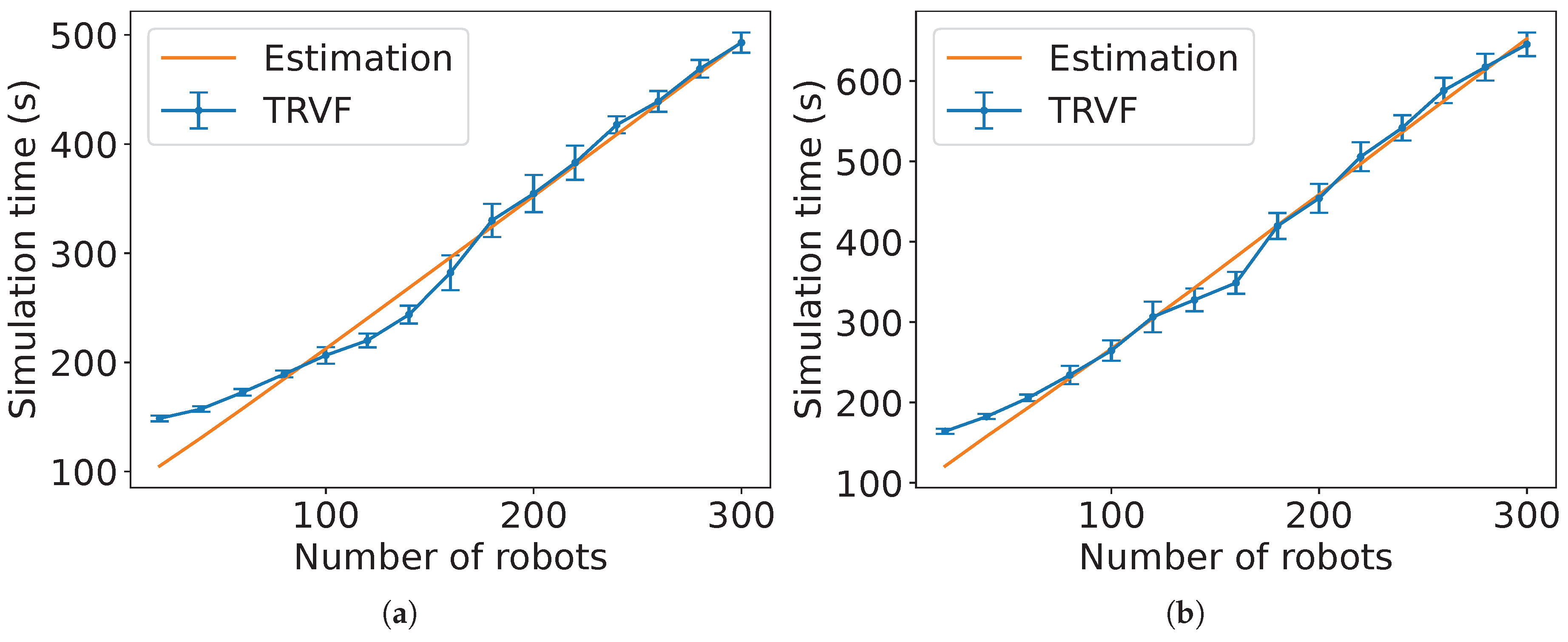
Figure 32.
Normalised root mean square error of the estimations in Figure 26, Figure 27, Figure 28, Figure 29, Figure 30 and Figure 31 for (a) holonomic and (b) non-holonomic robots.
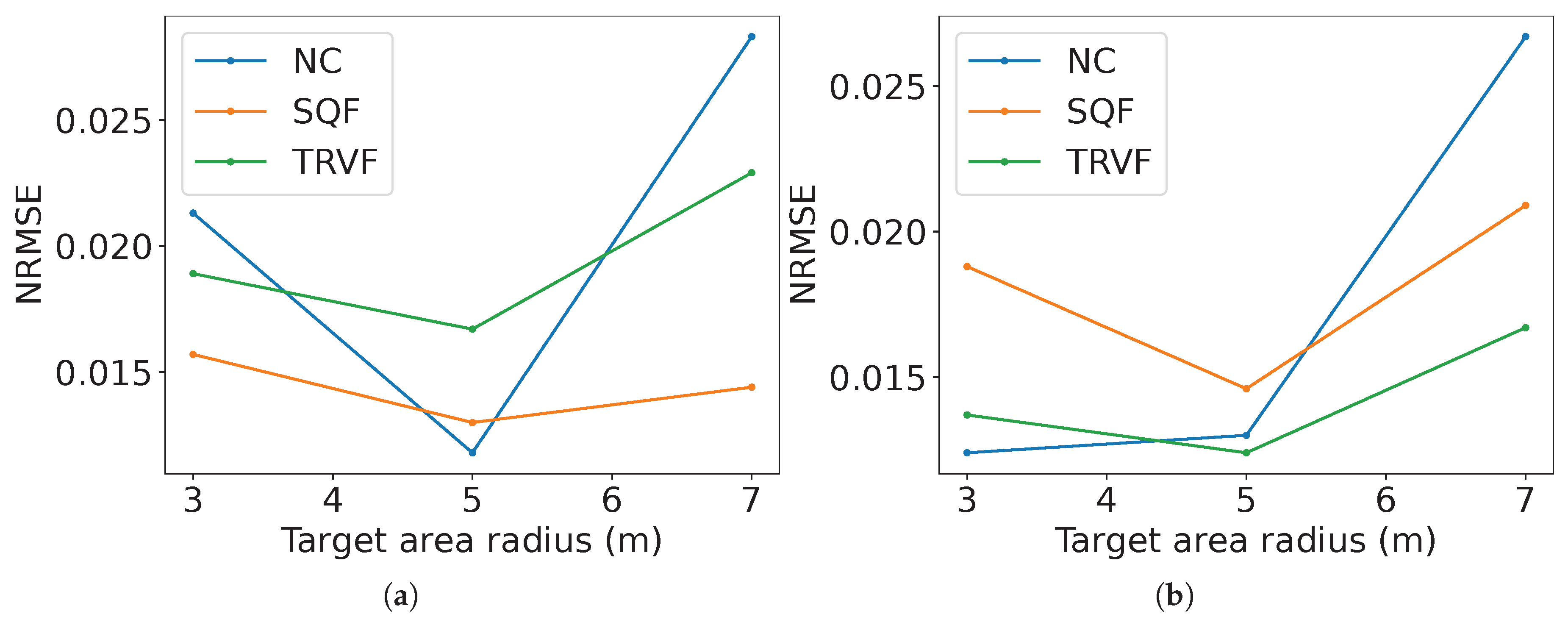
Figure 33.
Comparison of the linear speeds of the algorithms for m with (a) holonomic robots and (b) non-holonomic robots.
Figure 33.
Comparison of the linear speeds of the algorithms for m with (a) holonomic robots and (b) non-holonomic robots.
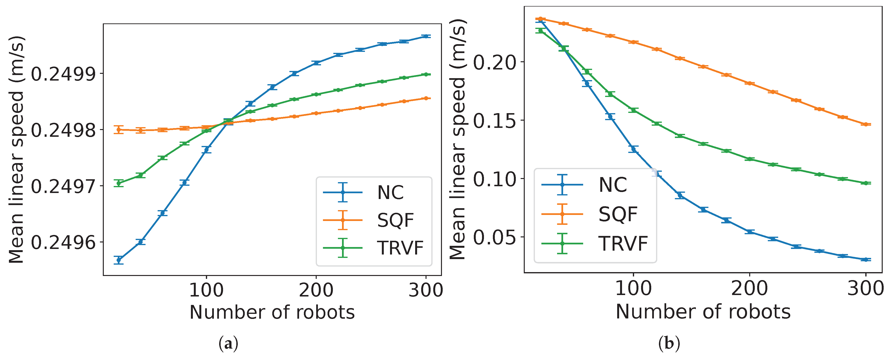
Figure 34.
Comparison of the mean distance between the robots of the algorithms for m with (a) holonomic robots and (b) non-holonomic robots.
Figure 34.
Comparison of the mean distance between the robots of the algorithms for m with (a) holonomic robots and (b) non-holonomic robots.
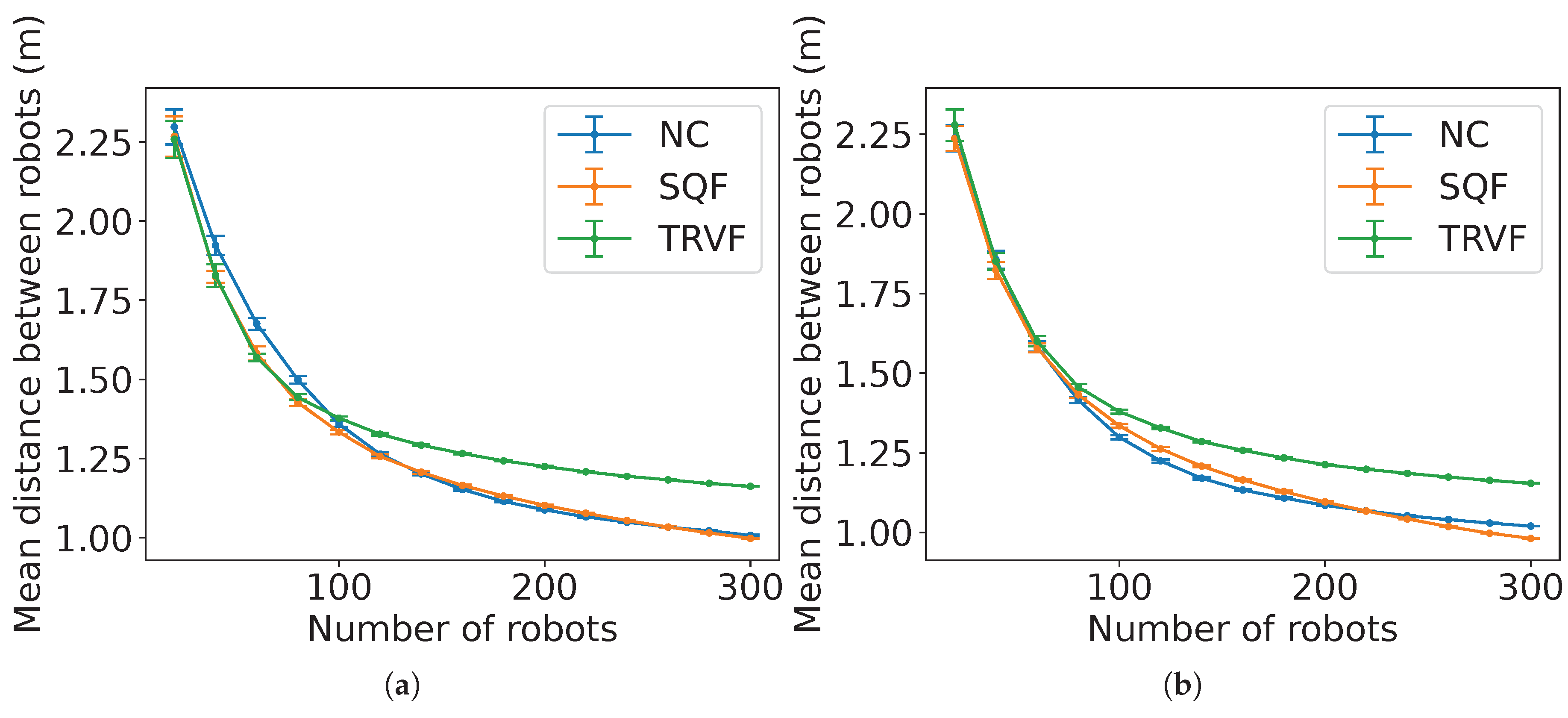
Figure 38.
Constants used for MT estimations ( and ) versus the percentage of robots in group A for the control algorithm of robots in group B (a) SQF and (b) TRVF. In the graphs, h and stand for holonomic and non-holonomic robots, respectively.
Figure 38.
Constants used for MT estimations ( and ) versus the percentage of robots in group A for the control algorithm of robots in group B (a) SQF and (b) TRVF. In the graphs, h and stand for holonomic and non-holonomic robots, respectively.
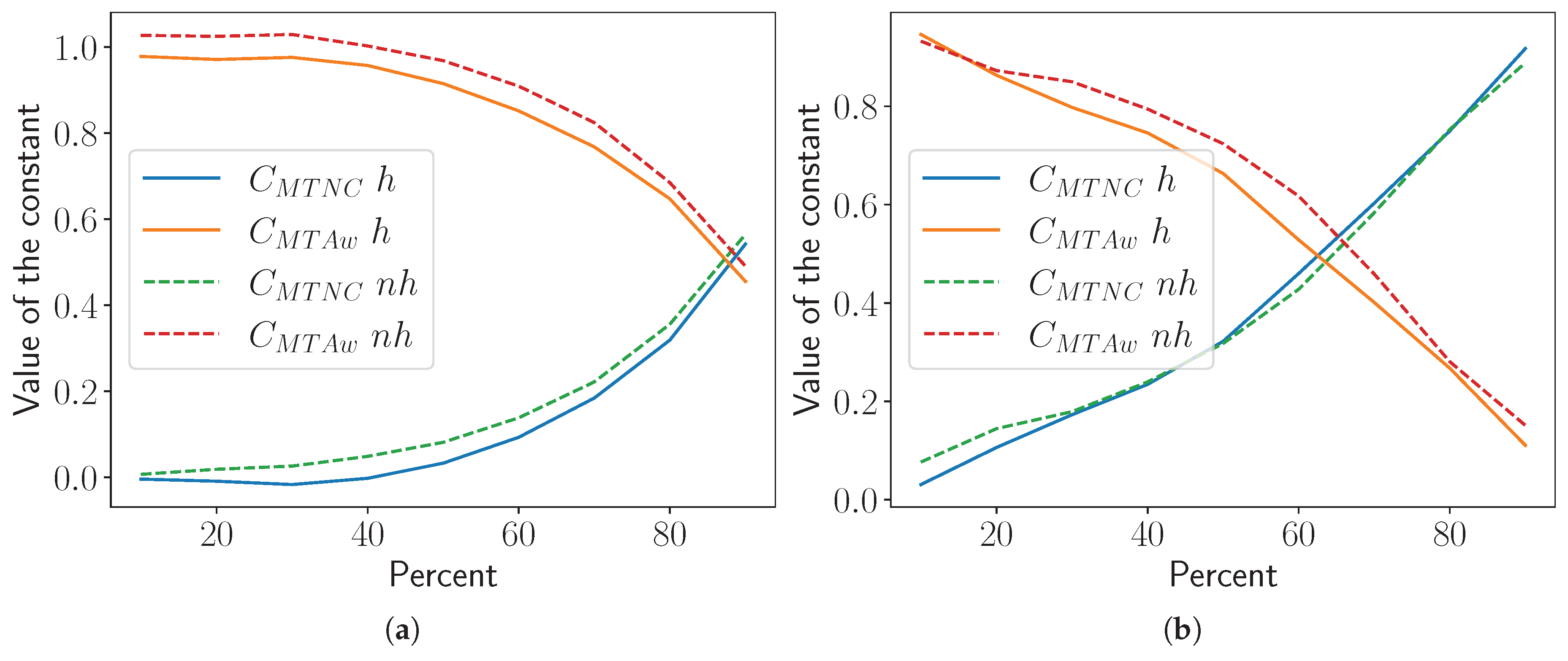

Table 1.
Summary of the variables commonly used in this work.
| Variable | Description | Variable | Description |
|---|---|---|---|
| The mean distance between the centre of mass of a robot and the others inside the influence radius for all robots. | Default influence radius. | ||
| D | Radius of the circular working area. | Constant magnitude of an attractive force. | |
| E | Maximum distance from the boundary of the working area for randomly positioning robots at the start of an experiment. | Multiplicative constant for the repulsive force. | |
| Expected task completion time of an algorithm . | N | Total number of robots in the swarm. | |
| Attractive force vector. | s | Radius of the common circular target area. | |
| Repulsive force vector. | Mean linear speed of all robots. | ||
| the common target position | |||
Table 2.
Default values for parameters used in all algorithms.
| s | D | E | |||||
|---|---|---|---|---|---|---|---|
| 3 m | 13 m | 8 m | 2.5 | 2.5 | 10 | 0.5 | 3 m |
Table 3.
Default values for the parameters used for TRVF algorithm.
| K | d | v | |||
|---|---|---|---|---|---|
| 5 | 3 m | 1 m/s | 3 | 1.1 | 1.1 |
Disclaimer/Publisher’s Note: The statements, opinions and data contained in all publications are solely those of the individual author(s) and contributor(s) and not of MDPI and/or the editor(s). MDPI and/or the editor(s) disclaim responsibility for any injury to people or property resulting from any ideas, methods, instructions or products referred to in the content. |
© 2025 by the authors. Licensee MDPI, Basel, Switzerland. This article is an open access article distributed under the terms and conditions of the Creative Commons Attribution (CC BY) license (http://creativecommons.org/licenses/by/4.0/).
Copyright: This open access article is published under a Creative Commons CC BY 4.0 license, which permit the free download, distribution, and reuse, provided that the author and preprint are cited in any reuse.


