Submitted:
02 September 2025
Posted:
04 September 2025
You are already at the latest version
Abstract
In this paper, we introduce and validate ECA110-Pooling, a novel rule-based pooling operator for Convolutional Neural Networks inspired by elementary cellular automata. A systematic comparative study is conducted, benchmarking ECA110-Pooling against conventional pooling methods (MaxPooling, AveragePooling, MedianPooling, MinPooling, KernelPooling) as well as state-of-the-art (SOTA) architectures. Experiments on three benchmark datasets-ImageNet (subset), CIFAR-10, and Fashion-MNIST-across training horizons ranging from 20 to 50,000 epochs demonstrate that ECA110-Pooling consistently achieves higher Top-1 accuracy, lower error rates, and stronger F1-scores than traditional pooling operators, while maintaining computational efficiency comparable to MaxPooling. Furthermore, in direct comparison with SOTA models, ECA110-Pooling delivers competitive accuracy with substantially fewer parameters and reduced training time. These results establish ECA110-Pooling as a validated and principled approach for image classification, bridging the gap between fixed pooling schemes and complex deep architectures. Its interpretable, rule-based design underscores both theoretical relevance and practical applicability in scenarios requiring a balance of accuracy, efficiency, and scalability.
Keywords:
Convolutional Neural Networks (CNNs)
; image classification
; pooling strategies
; MaxPooling
; AveragePooling
; MedianPooling
; MinPooling
; KernelPooling
; elementary cellular automata (ECA)
; ECA110-based pooling
; deep learning
; pattern recognition
; state-of-the-Art (SOTA) methods
; ANOVA
; computational efficiency
1. Introduction
Pooling layers represent a cornerstone in the architecture of Convolutional Neural Networks (CNNs), serving as a mechanism to progressively reduce the spatial resolution of feature maps while retaining their most salient information. By compressing representations in this manner, pooling layers not only enhance computational efficiency but also provide translational invariance and mitigate overfitting through dimensionality reduction. The conceptual foundations of hierarchical feature abstraction in neural networks can be traced back to Fukushima’s Neocognitron [1], while the optimization of such architectures became feasible following the introduction of backpropagation [2,3]. Among classical approaches, MaxPooling remains the de facto standard, largely due to its capacity to preserve dominant activations that improve recognition accuracy in large-scale image classification tasks such as ImageNet [4,5]. Nonetheless, the heavy reliance on MaxPooling is not without drawbacks. Alternative fixed operators have sought to mitigate these limitations: AveragePooling emphasizes global context at the expense of local discriminative detail [6], while MedianPooling introduces robustness to local noise and outlier activations, making it particularly suited for grayscale or noisy datasets [7]. In parallel, the field has witnessed the development of learnable pooling mechanisms. For example, KernelPooling introduces parameterized kernels that adaptively learn spatial aggregation, thereby tailoring pooling to task-specific distributions [8]. Other directions, such as stochastic pooling [9] and strided convolutions that eliminate pooling altogether [10], reflect broader efforts to optimize or bypass fixed downsampling operators. These methods, while often powerful, introduce additional computational costs and may complicate training pipelines. Beyond data-driven parameterization, biologically and mathematically inspired pooling strategies have emerged as a promising frontier. In particular, the incorporation of Elementary Cellular Automata (ECA) rules into CNNs provides a lightweight, rule-based alternative for encoding local dependencies prior to reduction. Rule 110 is especially noteworthy due to its proven computational universality and emergent complexity [11,12,13]. By embedding ECA transformations within CNNs, pooling layers such as the proposed ECA110-Pooling can capture rich micro-pattern interactions that conventional operators often discard [14,15]. This approach integrates theoretical rigor with practical utility, bridging symbolic dynamics and deep learning. Despite this diversity of proposals, systematic and controlled comparative evaluations remain limited. Much of the CNN literature continues to employ MaxPooling by default, often without explicit justification or consideration of task-specific requirements [16,17]. Recent surveys and benchmarking efforts emphasize the importance of revisiting such design choices, particularly as modern classification pipelines increasingly operate under constraints of efficiency, generalization, and robustness [18,19,20]. The motivation for this study is therefore twofold: (1) to rigorously compare a broad spectrum of pooling strategies-including MaxPooling, AveragePooling, MedianPooling, MinPooling, KernelPooling, and the novel ECA110-Pooling-within a uniform experimental framework across CIFAR-10, Fashion-MNIST, and ImageNet (subset); and (2) to examine not only predictive performance but also computational efficiency, feature retention, and robustness under diverse training horizons. By situating ECA110-Pooling against both traditional operators and state-of-the-art (SOTA) image classification baselines, this work provides a nuanced perspective on how pooling strategies influence the effectiveness and efficiency of CNN-based classification.
Contributions. This work advances the understanding of downsampling mechanisms in CNNs through the following contributions:
- Systematic comparative evaluation. We present a rigorously controlled comparison of six pooling operators-MaxPooling, AveragePooling, MedianPooling, MinPooling, KernelPooling, and the proposed ECA110-Pooling-within a shared CNN backbone, fixed training protocol, and identical hyperparameter settings, thereby isolating the impact of the pooling mechanism.
- Novel ECA110-based pooling mechanism. We introduce and formalize a pooling operator derived from Elementary Cellular Automata (Rule 110). The design follows a compact transform-reduce paradigm, enabling the preservation of discriminative local structures with minimal computational overhead.
- Learnable baseline for reference. The inclusion of KernelPooling as a parametric baseline allows a fair comparison between rule-based and learnable pooling approaches, highlighting the trade-offs between flexibility, accuracy, and efficiency.
- Comprehensive benchmarking across datasets and epochs. Pooling methods are evaluated on CIFAR-10, Fashion-MNIST, and ImageNet (subset), with training horizons ranging from 20 to 50,000 epochs. Metrics include Top-1 Accuracy, Error Rate, F1-score, per-epoch runtime, and model size, thereby providing a holistic assessment across simple and complex visual domains.
- Statistical and computational validation. Findings are validated through statistical tests (one-way ANOVA, Tukey’s HSD, Wilcoxon signed-rank, and paired t-tests) as well as computational profiling of convergence and efficiency trade-offs. This ensures that conclusions are both statistically robust and practically reproducible.
In summary, this study establishes ECA110-Pooling as a principled, lightweight, and competitive alternative to classical and learnable pooling mechanisms, with implications for advancing image classification across both high-capacity computational infrastructures and resource-constrained environments.
2. Related Work
Pooling operations have been extensively investigated in the design of Convolutional Neural Networks (CNNs) due to their central role in spatial downsampling, complexity reduction, and the promotion of translational invariance [21]. The earliest pooling operators, namely MaxPooling and AveragePooling, remain dominant in practice because of their simplicity and efficiency. However, these fixed operators exhibit inherent limitations, such as the loss of fine-grained details or increased sensitivity to noise, which has motivated a diverse range of extensions. One line of work has introduced stochasticity or adaptivity to the pooling process. Stochastic pooling selects activations in proportion to their magnitudes, providing an implicit regularization effect that enhances generalization. Mixed pooling and gated pooling further improve flexibility by probabilistically combining or adaptively selecting between max and average pooling based on input data characteristics [22]. Meanwhile, adaptive pooling methods such as spatial pyramid pooling and region-of-interest pooling enable the extraction of fixed-size feature representations from variable input dimensions, making them indispensable for object detection and recognition pipelines. Another prominent direction replaces static operators with learnable downsampling mechanisms. Strided convolutions have been proposed as pooling-free alternatives that maintain convolutional structure while performing resolution reduction [23]. Parametric pooling methods, including -integration pooling [24], extend the flexibility of classical operators by introducing tunable parameters, while generalized pooling approaches provide continuous interpolations between max and average pooling [25]. These advances reflect a growing emphasis on adaptive downsampling, where the pooling function itself becomes optimized jointly with the network. Surveys of pooling methods confirm that such operator-level choices can significantly influence model generalization and robustness, depending on data distribution and task requirements [26]. More recently, pooling has been linked with the broader trend of incorporating attention mechanisms into CNNs. Residual attention networks combine pooling with attention-driven feature selection, enhancing representational capacity in hierarchical architectures. Surveys and empirical studies emphasize the effectiveness of attention-based pooling, which aggregates features according to learned importance weights rather than fixed heuristics [27,28,29]. This paradigm shift situates pooling within the broader landscape of context-sensitive aggregation, narrowing the gap between CNNs and Transformer-based vision architectures. Biologically and mathematically inspired operators remain less explored but present promising avenues. For example, Elementary Cellular Automata (ECA) provide a rule-based framework for capturing local structural dependencies in image data. Rule 110, with its proven computational universality and emergent complexity, has been adapted as a lightweight pooling mechanism (ECA110) capable of preserving micro-pattern interactions that are often lost in traditional pooling. Such operators bridge theoretical concepts with practical deep learning architectures, introducing new opportunities for interpretable yet efficient pooling designs. Complementary work has also examined hybrid and biologically inspired operators, including multiscale pooling strategies [30,31,32], binary pooling with attention [33], and probabilistic pooling designs [34], further diversifying the design space. Despite this rich body of work, most prior studies have evaluated pooling variants in isolation, typically comparing a new method against a small number of baselines under limited experimental conditions. As a result, systematic, large-scale benchmarks that place multiple pooling operators within identical CNN backbones, training regimes, and datasets remain scarce. This fragmentation obscures the true trade-offs among accuracy, computational cost, and generalization. To address this gap, the present study contributes a controlled and comprehensive comparative analysis of six pooling strategies-MaxPooling, AveragePooling, MedianPooling, MinPooling, KernelPooling, and the proposed ECA110-Pooling-across diverse datasets and training horizons, thereby advancing the empirical understanding of pooling as a fundamental component of image classification models.
3. Preliminaries and Theoretical Foundations
3.1. Convolutional Neural Networks
Convolutional Neural Networks (CNNs) constitute a fundamental paradigm in deep learning for analyzing data with grid-like topology, such as images and videos. Their development has been strongly influenced by architectural innovations and training methodologies that enabled deeper, more expressive models. Early contributions on efficient optimization, such as greedy layer-wise pretraining [35], provided a foundation for scaling neural networks before the advent of modern training techniques. A CNN is typically structured as a hierarchy of convolutional filters for feature extraction, interleaved with pooling or subsampling operations that reduce spatial resolution while preserving discriminative information. Such downsampling mechanisms contribute to translational invariance, a property critical for visual recognition. Complementary advances, including recurrent and memory-augmented architectures, extended the representational power of neural models beyond vision [36,37]. Over the past decade, CNNs have become the backbone of state-of-the-art systems in image classification, detection, and segmentation. Broader surveys and syntheses emphasize their central role in artificial intelligence and their interplay with other paradigms such as recurrent and attention-based networks [38,39]. These developments situate CNNs not only as feature extractors but as a cornerstone of modern deep learning.
3.2. Pooling Strategies: Formal Definitions
Let denote an input feature map, where H, W, and C represent height, width, and the number of channels, respectively. For a pooling window of size , centered (or positioned) at spatial coordinates in channel c, several pooling strategies can be formally defined as follows.
MaxPooling:
AveragePooling:
MedianPooling:
MinPooling:
KernelPooling.
KernelPooling represents an adaptive pooling mechanism in which the aggregation of local activations is guided by learnable spatial kernels. Unlike fixed pooling operators such as MaxPooling or AveragePooling, where the aggregation rule is predetermined, KernelPooling jointly optimizes the kernel weights with the rest of the Convolutional Neural Network during training, thereby enabling task-specific spatial information retention. Formally, let denote an input feature map with C channels. Each channel c is associated with a learnable pooling kernel , where k is the spatial extent of the pooling window. For each pooling region , positioned at location , the downsampled activation is defined as:
with stride s controlling the sampling rate across the feature map. This formulation unifies the concepts of filtering and subsampling within a single operation, allowing the network to learn optimal spatial aggregation patterns that balance feature selectivity and robustness to intra-class variability.
The pseudocode implementation in Algorithm 1 summarizes the iterative computation of downsampled activations. From a computational perspective, KernelPooling introduces an additional parameterization proportional to , which slightly increases training time per epoch compared to non-learnable pooling operators. Nevertheless, this overhead is often compensated by improved generalization performance, particularly in domains where the spatial distribution of discriminative features is complex and non-uniform.
| Algorithm 1:KernelPooling ( kernel, stride s) |
|
Input: Feature map ; learnable kernels
Output: Downsampled feature map y
fortoCdo
for over grid with stride sdo
|
4. ECA110-Based Pooling Mechanism for CNNs
4.1. Definition of ECA110-Pooling
The proposed ECA110-based pooling mechanism is inspired by the theoretical framework of Elementary Cellular Automata (ECA), focusing on Rule 110, which is well known for its computational universality and emergent structural complexity. Unlike conventional pooling operators-such as max or average pooling-that directly apply a reduction over local receptive fields, ECA110-based pooling employs a two-stage transform–reduce procedure, wherein a deterministic cellular automaton transformation precedes dimensionality reduction.
Formally, given a pooling window in channel c, activations are first rearranged into a one-dimensional vector:
The evolution function , corresponding to ECA Rule 110, is then applied to , yielding a transformed sequence that encodes local structural dependencies:
Finally, the pooled output is computed as the normalized sum:
4.2. Algorithm: ECA110-Pooling (Elementary Cellular Automaton Rule 110 Operator)
The ECA110 pooling operator (defined in the Algorithm 2) processes each local window in two stages: (i) a rule–based binary transformation that captures local interactions via the Elementary Cellular Automaton Rule 110, followed by (ii) a normalized-sum reduction. For each channel c and window (sampled with stride s), the feature values are flattened, binarized with respect to a threshold , evolved once (or for a fixed number of steps) under Rule 110, and then aggregated by averaging the transformed states.
Indicator function. The operator acts elementwise on a vector and returns a binary vector:
| Algorithm 2:ECA110-Pooling (window , stride s) |
|
Input: Output: fortoCdo for over spatial grid with stride sdo //Indicator-based binarization at threshold //Apply one (or T) Rule-110 evolution step(s) //Normalized-sum reduction (mean of transformed states) |
Typical choices for include the local mean or median of the window, or a fixed hyperparameter shared across windows. The parameter T denotes the number of iterations of Rule 110 applied to the binarized vector , with used as the default in our experiments. The function denotes the iterative application of Rule 110, an Elementary Cellular Automaton (ECA) characterized by its local update rule acting on triplets of binary states. Specifically (Table 1), ECA 110 maps each triplet to a new state according to the transition rule encoded by the binary pattern (110 in decimal). This automaton is notable for its computational universality and emergent structural complexity. In our framework, applies the update rule T times over the one-dimensional sequence , with a deterministic scan order induced by flatten. Boundary handling (fixed zeros) is consistently enforced across experiments.
4.3. Main Steps of ECA110-Pooling on Window
For a receptive field, ECA110-based pooling proceeds through the following steps (see Figure 1):
- 1.
- Flattening: The activations are extracted and arranged into a one-dimensional vector .
- 2.
- Binarization: Elements of are mapped into binary states via thresholding (relative to mean or median), producing .
- 3.
- Application of Rule 110: The binary sequence evolves according to the local update rule , generating .
- 4.
- Reduction: The normalized sum of provides the final pooled activation.
Illustrative Example of ECA110 Pooling on a window.
Consider the following local window extracted from a feature map (channel c):
- 1.
- Flattening. The window is rearranged into a one-dimensional vector:
- 2.
- Binarization. Using the mean of the window () as threshold, values are mapped to 1 and those to 0:
- 3.
- Application of Rule 110. The binary sequence is evolved according to the update function . For illustration, after one iteration step the transformed sequence is:
- 4.
- Reduction by normalized summation. The final pooled activation is computed as:
Thus, the output of ECA110 pooling for this window is . This demonstrates how the operator embeds a deterministic rule-based transformation prior to normalized reduction, thereby encoding non-linear structural dependencies before aggregation.
Observation 1
(Alternative Reduction Strategies for ECA110-Pooling). While the normalized sum (mean pooling) is the default reduction strategy in ECA110-Pooling, several alternatives can be employed depending on the task and robustness requirements. Given the transformed vector obtained after the application of Rule 110, the pooled output y may be defined using one of the following reduction operators:
- Normalized Sum (Mean Pooling):
- Maximum / Minimum Reduction:
- Weighted Mean Reduction: with learnable or fixed weights :
- Median Reduction:
- -Norm Reduction: where corresponds to the mean and approaches the maximum.
- Entropy-Based Reduction: measuring the diversity of the transformed activations: where ϵ is a small constant for numerical stability.
- Learnable Reduction (Attention / MLP): In more flexible designs, y can be obtained through a learnable function such as attention pooling or a small neural layer , where g is trained jointly with the CNN backbone.
These alternatives highlight the extensibility of the ECA110-Pooling framework, allowing it to adapt to different robustness, efficiency, or generalization requirements.
The proposed ECA110-based pooling operator extends the conventional downsampling paradigm in Convolutional Neural Networks by introducing a deterministic, rule-driven transformation prior to reduction. Through the application of the Elementary Cellular Automaton Rule 110, the operator captures fine-grained non-linear local interactions that are typically discarded by classical pooling mechanisms such as max or average pooling. This design enables CNNs to preserve structural dependencies and spatial dynamics that are critical for precise feature extraction, thereby enhancing robustness in image classification tasks where subtle local variations play a decisive role. Although it introduces a modest but constant computational overhead, the method remains efficient while providing a principled and theoretically grounded alternative to conventional pooling operators. Consequently, ECA110-Pooling has the potential to enrich representational capacity and improve generalization performance across diverse visual recognition benchmarks.
5. Experimental Framework
5.1. Datasets, Data Splits, and Training Setup
To enable a systematic and unbiased comparative evaluation, three widely adopted benchmark datasets were employed: ImageNet (subset), CIFAR-10, and Fashion-MNIST (Table 2). These datasets were selected to capture a wide spectrum of visual characteristics, resolutions, and intra-class variability, thereby ensuring a robust assessment of pooling strategies across different levels of complexity.
To assess robustness under varying data availability, three consistent train/test splits were employed across all datasets (Table 3). These complementary cases provide insight into how pooling mechanisms, particularly the proposed ECA110 operator, adapt to both data-rich and data-constrained scenarios.
All models were trained using a unified optimization protocol to ensure fairness across pooling variants. The Adam optimizer was adopted, coupled with the categorical cross-entropy loss function. Training was performed with a mini-batch size of 64. To investigate performance across different learning regimes, the number of epochs was systematically varied over the range: This schedule captures short-term convergence dynamics, mid-range performance stabilization, and long-term learning behavior, thereby enabling a comprehensive evaluation of pooling strategies under diverse experimental conditions. Importantly, both the dataset partitioning and the training protocol were applied identically across all pooling operators, ensuring that observed differences in performance can be attributed solely to the pooling mechanism under evaluation.
5.2. CNN - Network Architecture
To isolate the influence of the pooling operator, all experiments were conducted using an identical convolutional neural network (CNN) backbone. The design is compact yet expressive, ensuring efficient feature extraction without introducing unnecessary architectural complexity. The adopted configuration consists of:
- A first convolutional layer with 64 filters of size , followed by the evaluated pooling operator.
- A second convolutional layer with 128 filters of size , again followed by the selected pooling operator.
- A fully connected (FC) layer with 256 units, culminating in a Softmax output layer for multi-class classification.
This architectural constraint ensures that observed differences in performance can be attributed directly to the pooling mechanisms rather than confounding factors such as network depth, receptive field, or parameterization.
5.3. Algorithmic Framework
The methodology was formalized through the following algorithmic components:
- 1.
-
Training and Evaluation Algorithm. Algorithm 3 details the training procedure of a CNN with interchangeable pooling operators . Metrics including Top-1 accuracy, training time per epoch, and model size were systematically recorded.The components and functionality of the Algorithm 3 can be described as follows:
- −
- Inputs and Outputs: The algorithm takes as input datasets (collections of labeled samples used for training and validation), number of classes K, pooling type , training epochs E, and optimization hyperparameters: learning rate , momentum m, and weight decay . The outputs are the trained model and evaluation metrics (Top-1 accuracy, time/epoch, model size).
- −
- Network Initialization: The CNN backbone is fixed across experiments, differing only in the pooling operator: Conv1 (, 64 filters) → ReLU → Pool1() → Conv2 (,128 filters) → ReLU → Pool2() → Flatten → FC(256) → ReLU → FC(K) → Softmax. ReLU (Rectified Linear Unit) introduces non-linearity by suppressing negative activations, while Softmax produces a normalized probability distribution over the K output classes. The pooling operator P, applied with window size k and stride s, represents the sole interchangeable element within the otherwise fixed backbone. This design ensures that observed performance variations are attributable primarily to the pooling mechanism rather than architectural or parametric differences.
- −
- Optimization: Training uses SGD with learning rate , momentum m, and weight decay . The cross-entropy loss is computed as with standard gradient update steps (zero_grad(), backward(), step()). The called functions here have the following attributes- CrossEntropy(): computes the negative log-likelihood loss on one-hot labels or class indices. zero_grad(): resets all previously accumulated gradients; backward(): performs backpropagation, accumulating gradients with respect to network parameters; step(): updates model parameters using the SGD rule with momentum and weight decay. Stochastic Gradient Descent (SGD) iteratively minimizes the loss by computing parameter updates from mini-batches, with momentum accelerating convergence and weight decay acting as regularization.
- −
- Training Loop: For each epoch : (i) batches are forwarded through the network (Forward()), loss is computed and parameters updated; (ii) validation is performed on , logging Top-1 accuracy, time/epoch, and model size.
- 2.
- Forward Pass. Algorithm 4 specifies the forward propagation pipeline, where feature maps are progressively transformed through convolution, nonlinearity, pooling, and classification layers. The function Forward() applies: (i) convolutional layers (Conv2D with filters) for local feature extraction; (ii) ReLU activations to introduce non-linearity by suppressing negative responses; (iii) the interchangeable pooling operator P with window and stride , responsible for spatial downsampling; (iv) flattening of feature maps into a vector representation; (v) fully connected layers (FC) for global integration of features, followed by a final Softmax that converts logits into class probabilities , where logits denote the raw, unnormalized outputs of the final fully connected layer. The pooling operator Pool() supports three cases: (a) standard operators (max, average, median, min), (b) learnable weighted aggregation in KernelPooling, and (c) a transform–reduce scheme in ECA110, which consists of flattening, binarization via , evolution under Rule 110, and normalized-sum reduction. This modular design ensures that performance differences can be directly attributed to the pooling operator under evaluation.
- 3.
- Pooling Operator. Algorithm 5 defines the pooling layer implementation, where the input tensor has four components: B denotes the batch size, C the number of channels, H the height, and W the width of the feature maps. The operator is parameterized by the pooling type P, the window size k, and the stride s. For standard operators (), the algorithm applies the corresponding reduction function over each local region. In the case of KernelPooling, each channel c is associated with a learnable kernel , enabling adaptive weighted aggregation of local activations. For the proposed ECA110-Pooling, a transform–reduce framework is employed: each local window is flattened into a vector , binarized through a threshold , and then evolved for T iterations under Elementary Cellular Automaton Rule 110. The transformed sequence is subsequently reduced via normalized summation, producing the scalar output for each spatial location. Unless otherwise specified, the our default choice is . This unified formulation allows the Pool() function to encompass conventional, learnable, and automaton-driven mechanisms within a single modular framework, facilitating rigorous and fair comparisons across pooling strategies.
This integrated methodology ensures consistency across datasets, data splits, and training conditions, allowing for a fair and clear comparison between different pooling methods.
| Algorithm 3:Training and Evaluating a CNN with a Pluggable Pooling Operator |
|
Input: Datasets , number of classes K, pooling type , epochs E, learning rate , momentum m, weight decay
Output: Trained model; metrics: Top-1 accuracy, time/epoch, model size
Network initialization: Conv1: , 64 filters; ReLU Pool1: P with window , stride Conv2: , 128 filters; ReLU Pool2: P with window , stride Flatten → FC(256) → ReLU → FC(K) → Softmax
Optimization setup: SGD; loss: CrossEntropy
fortoEdo
//— Training phase —foreachbatch in do zero_grad(); backward(); step() //— Validation phase — Evaluate: compute Top-1 on ; log time/epoch and model size |
| Algorithm 4:Forward |
|
return |
| Algorithm 5:Pool (X has shape ) |
|
Result: U with shape
ifthen
return the corresponding standard operator with window and stride s
else
ifthen//KernelPooling: learnable weighted aggregation fordo (learnable parameters) returnU ifthen //ECA110: transform–reduce with Rule 110 and normalized sum fordo Extract window //threshold //indicator function //apply T evol. steps; by default //normalized sum (mean) returnU |
5.4. Evaluation Metrics
To ensure a rigorous and comprehensive assessment of pooling operators, multiple evaluation metrics were employed, designed to capture both predictive performance and computational efficiency. These metrics collectively provide a balanced perspective on accuracy, robustness, and computational trade-offs.
- Top-1 Classification Accuracy. The primary metric, reflecting the proportion of test samples for which the predicted class with the highest probability matches the ground truth. This directly measures the discriminative capacity of pooling operators in image classification.
- Error Rate. Defined as the complement of Top-1 Accuracy (), this metric emphasizes the proportion of misclassified samples and provides an intuitive measure of classification mistakes.
- F1-Score. The harmonic mean of precision and recall, balancing false positives and false negatives. This is particularly useful for datasets with class imbalance, providing a more nuanced view of predictive performance beyond raw accuracy.
- Training Time per Epoch. The average wall-clock time required to complete one training epoch, providing insight into the computational overhead introduced by each pooling strategy.
- Model Size. The number of trainable parameters stored in memory, reported in megabytes (MB). This is particularly relevant for learnable pooling mechanisms such as KernelPooling, which increase parameterization.
- Convergence Behavior. The stability and rate at which training accuracy and loss curves converge across epochs, capturing optimization dynamics under different pooling strategies.
- Statistical Significance. Observed performance differences were validated using statistical tests across multiple runs: one-way ANOVA with Tukey’s HSD post-hoc test, complemented by paired comparisons (Wilcoxon Signed-Rank and paired t-test). This ensures the robustness and reliability of comparative conclusions.
Table 4 summarizes the evaluation metrics and their specific role in assessing pooling operators within the experimental framework.
6. Experimental Results
This section presents the empirical findings from the comparative evaluation of pooling operators across the three benchmark datasets: ImageNet (subset), CIFAR-10, and Fashion-MNIST. Results are consistently reported under the three data-splitting scenarios (80/20, 65/35, and 50/50) and training schedules described in Section 4. The analysis focuses on the discriminative capability, convergence dynamics, and computational efficiency of the proposed ECA110-based pooling operator in comparison with both conventional and learnable pooling schemes.
6.1. Classification Performance Across Epochs
Table 5, Table 6 and Table 7 provide a detailed comparison of Top-1 accuracy, error rate, and F1-score across training epochs for the three benchmark datasets. Several trends can be observed:
- ECA110-Pooling consistently surpasses MinPooling and MedianPooling across all epochs, while providing performance on par with or superior to MaxPooling and AveragePooling.
- KernelPooling occasionally matches the accuracy of ECA110, but incurs a larger model size and increased training time.
- The performance advantage of ECA110 is most pronounced under the 50/50 split condition, highlighting its ability to generalize effectively in low-data regimes.
- Long-term training schedules () stabilize the superiority of ECA110, with diminishing returns observed for standard pooling operators.
Cross-dataset comparison. Figure 2 aggregates performance trends across all three datasets. The figure reports averaged Top-1 Accuracy, Error Rate, and F1-score for each pooling operator over different training horizons. The results confirm that:
- ECA110-Pooling achieves the best overall balance across datasets, with the highest accuracy and F1-score, and the lowest error rate.
- KernelPooling is competitive but consistently lags in efficiency due to its parameter overhead.
- MinPooling is systematically the weakest operator, while MedianPooling provides limited robustness in noisy or grayscale settings.
To condense the detailed experimental results, Table 8 reports the aggregated performance of all pooling operators across ImageNet (subset), CIFAR-10, and Fashion-MNIST. The table summarizes mean Top-1 Accuracy, Error Rate, and F1-score, thereby providing a compact view of the overall discriminative capacity of each method. Results confirm that ECA110-Pooling achieves the best trade-off, with consistently higher accuracy and F1-scores, while also reducing the error rate compared to both classical and learnable alternatives.
6.2. Convergence Dynamics
The convergence behavior of training across pooling operators was systematically examined on ImageNet (subset), CIFAR-10, and Fashion-MNIST. Conventional operators such as MaxPooling and AveragePooling display rapid early improvements but frequently plateau after approximately 500– epochs, indicating limited representational flexibility once dominant activations have been captured. MedianPooling exhibits slightly more stable convergence, while MinPooling lags significantly in both speed and final accuracy. In contrast, the proposed ECA110-Pooling consistently demonstrates gradual and sustained improvements across extended training schedules, including long runs of and epochs. This stability suggests that the automaton-driven transform–reduce mechanism preserves local structural dependencies over time, thereby facilitating richer feature representations. KernelPooling achieves comparable late-stage performance but at the cost of increased parameterization and slower epoch times. Figure 3 provides a comparative overview of convergence curves for all three datasets across the range of training epochs (20 to 50,000). The visualization highlights that while conventional operators tend to stagnate, ECA110-Pooling maintains progressive accuracy gains, thereby confirming its ability to sustain long-term learning and improve generalization under both data-rich and data-constrained conditions. Overall, convergence analysis confirms that ECA110-Pooling supports robust long-term learning dynamics, avoiding premature stagnation and achieving superior performance relative to conventional pooling schemes.
6.3. Computational Complexity
A complexity analysis of the six pooling strategies is provided to highlight their computational overhead before practical evaluation. Let denote the pooling window size and C the number of channels in the feature map. The per-window complexity can be summarized as follows:
- MaxPooling, AveragePooling, MedianPooling, MinPooling. Each of these operators requires evaluating all activations within the pooling window for every channel, resulting in a computational cost of MedianPooling incurs an additional constant sorting factor per window but remains of the same asymptotic order.
- KernelPooling. This operator performs a weighted sum of activations using learnable kernels of size per channel. The computational cost is therefore identical to the classical operators, but it introduces additional parameters, which increase memory usage and training time due to gradient updates.
- ECA110-Pooling. The proposed operator first binarizes the window and then evolves it for T iterations under Rule 110 before applying a reduction. This yields a per-window cost of where T is the number of automaton steps. Since T is a small constant in practice (e.g., in our experiments), the complexity remains effectively linear in , incurring only a modest constant-time overhead relative to standard pooling.
Overall, all six pooling operators share the same asymptotic order of growth, , with KernelPooling distinguished by its additional learnable parameters and ECA110-Pooling by a lightweight constant-factor expansion due to cellular automaton iterations. This analysis explains the results observed, where ECA110 achieves near-MaxPooling efficiency while surpassing it in predictive performance.
The complexity profile summarized in Table 9 and illustrated in Figure 4 highlights that, although all pooling strategies share the same asymptotic order , practical distinctions arise in constant factors and parameterization. KernelPooling increases memory and training cost due to its learnable weights, while MedianPooling incurs a modest runtime penalty from sorting. In contrast, ECA110-Pooling introduces only a negligible constant-time overhead, despite the transformation based on the cellular automaton rules. These observations anticipate the empirical results in the next subsection, where we show that ECA110 achieves a favorable trade-off between accuracy gains and runtime efficiency.
6.4. Computational Efficiency
Efficiency results are summarized in Table 10, which reports the average training time per epoch and model size across the three benchmark datasets (ImageNet subset, CIFAR-10, and Fashion-MNIST). The table highlights the trade-offs between computational cost and architectural complexity for each pooling operator.
The following observations can be drawn:
- Standard pooling operators (Max, Average, Min, Median) are efficient in terms of both execution time and memory footprint.
- KernelPooling significantly increases model size due to its learnable kernels, which, although beneficial for accuracy in some scenarios, introduce a notable computational burden.
- ECA110-Pooling introduces only a modest and stable overhead compared to non-learnable baselines, while remaining substantially more efficient than KernelPooling.
- Importantly, ECA110’s computational overhead is invariant to dataset size, a direct consequence of its rule-driven local design.
To complement the tabular results, Figure 5 provides a direct comparison between average epoch times and achieved classification accuracy for all six pooling methods. The figure illustrates the trade-off between computational efficiency and predictive performance, highlighting that ECA110 consistently achieves the highest accuracy with only marginal runtime overhead, whereas KernelPooling delivers competitive accuracy at substantially higher computational cost.
6.5. Statistical Validation
To rigorously assess the reliability of the observed performance differences, we conducted a series of statistical validation procedures across five independent runs per configuration. These included both parametric and non-parametric analyses, thereby ensuring robustness under different distributional assumptions.
6.6. Statistical Validation
To rigorously assess the reliability of the observed performance differences, we conducted a series of statistical validation procedures across five independent runs per configuration. These included both parametric and non-parametric analyses, thereby ensuring robustness under different distributional assumptions. In a one-way ANOVA, the between-group degrees of freedom are given by and the within-group (residual) degrees of freedom by , where k is the number of groups and N the total number of observations. In this work, pooling operators (MaxPooling, AveragePooling, MedianPooling, MinPooling, KernelPooling, and ECA110-Pooling). Each operator was evaluated using five independent runs per dataset–split–epoch configuration, yielding observations in total. Consequently, the ANOVA results report Between-group df = 5 and Within-group df = 24. A one-way Analysis of Variance (ANOVA) was applied to compare mean classification accuracy across pooling operators for each dataset, split ratio, and training epoch. The results, summarized in Table 11, revealed statistically significant differences () across almost all experimental conditions, spanning ImageNet (subset), CIFAR-10, and Fashion-MNIST. Notably, significance was observed as early as 20 epochs and became more pronounced with longer training, indicating that pooling choice consistently impacted learning outcomes. Following ANOVA, post-hoc analysis was carried out using Tukey’s Honestly Significant Difference (HSD) test to identify which pooling operators accounted for the observed differences. The results, reported in Table 12, highlight that ECA110-Pooling (ECA) significantly outperformed conventional operators at mid and late training stages. For instance, at 500 and 5000 epochs, ECA showed consistent gains over MaxPooling, AveragePooling, and MinPooling across all datasets and split ratios. In contrast, at very early epochs (e.g., 20), the differences were less pronounced, with some cases showing MaxPooling or MedianPooling outperforming only MinPooling. These findings suggest that ECA’s benefits manifest more strongly as training progresses. To complement the ANOVA and Tukey HSD analyses, paired t-tests were conducted between ECA and each baseline pooling operator, with results presented in Table 13. The t-tests confirmed that ECA’s improvements were statistically significant () in the majority of cases. Particularly, CIFAR-10 exhibited strong advantages for ECA over MinPooling and AveragePooling across all splits, while ImageNet demonstrated significant improvements over MaxPooling and AveragePooling at later epochs (500 and 5000). Fashion-MNIST results were consistent with this trend, showing robust superiority of ECA under both balanced and reduced splits. Recognizing that neural network performance distributions may deviate from normality, we further validated results using the non-parametric Wilcoxon signed-rank test. As shown in Table 14, the Wilcoxon results corroborated the t-test outcomes, reinforcing that ECA’s performance improvements are systematic rather than artifacts of distributional assumptions. Importantly, ECA consistently outperformed MinPooling across all datasets, and at later epochs it also surpassed MaxPooling and AveragePooling with high significance. Taken together, the convergence of results across four complementary statistical tests provides strong evidence that ECA110-Pooling yields reliable improvements. The analysis confirms that its advantages are not confined to specific datasets or splits but generalize across conditions, with the most pronounced gains observed in data-constrained regimes (65/35 and 50/50 splits) and at longer training horizons. These findings establish ECA110-Pooling as a statistically validated alternative to conventional pooling mechanisms, offering both accuracy and robustness benefits across diverse image classification tasks.
6.7. Benchmarking ECA110-Pooling Against State-of-the-Art Methods
To further contextualize the effectiveness of ECA110-Pooling, we benchmark its performance against representative state-of-the-art (SOTA) architectures under identical experimental conditions. The selected methods include ResNet-50 [40], DenseNet-121 [41], EfficientNet-B0 [42], MobileNetV2 [43], and the Vision Transformer (ViT-Small) [44]. All results were obtained from consistent reimplementations using the same data splits (80/20, 65/35, 50/50) and the same number of training epochs (500, 5000, and 10000 epochs), thus ensuring a fair and unbiased comparison across pooling-based and SOTA-based methods.
Table 15 reports Top-1 Accuracy, Error Rate, and F1-score across ImageNet (subset), CIFAR-10, and Fashion-MNIST.
From these results, several observations emerge:
- On Fashion-MNIST, ECA110-Pooling not only matches but occasionally surpasses SOTA models, confirming its robustness in grayscale image classification tasks.
- On CIFAR-10, ECA110 closely approaches the performance of ResNet and DenseNet at extended training horizons (5000+ epochs), while maintaining substantially lower computational cost, positioning it as a highly competitive solution in resource-constrained settings.
- On ImageNet (subset), although large-scale models such as EfficientNet-B0 and DenseNet remain superior in absolute accuracy, ECA110 significantly narrows the gap under reduced-data splits (65/35 and 50/50). This demonstrates its strong generalization capability when training data are scarce. Importantly, this advantage is achieved with markedly lower parameterization and training time compared to heavyweight models like ResNet-50, DenseNet-121, or EfficientNet-B0.
Table 16 provides a comparative analysis of the parameterization requirements and memory footprint associated with different pooling methods and SOTA architectures. By “memory footprint,” we refer to the storage space required for model parameters (weights and biases), typically measured in megabytes (MB), which reflects both disk storage requirements and memory consumption during training and inference. Classical pooling operators (MaxPooling, AveragePooling, MedianPooling, MinPooling) and the proposed ECA110-Pooling do not introduce additional trainable parameters, thereby resulting in a negligible memory footprint. KernelPooling, while adding flexibility through learnable kernels, incurs a modest increase in model size. In contrast, state-of-the-art architectures such as ResNet-50, DenseNet-121, EfficientNet-B0, MobileNetV2, and ViT-Small require millions of parameters, with memory footprints ranging from tens to hundreds of MB. This contrast underscores the lightweight nature of ECA110-Pooling, which achieves competitive image classification performance without incurring the significant computational and storage costs typically associated with large-scale deep learning architectures.
To complement these tabular comparisons, Figure 6 illustrates the trade-off between performance and efficiency. The diagram reports the average Top-1 Accuracy across all datasets, splits, and training horizons, alongside computational costs expressed as average epoch time (seconds) and model size (MB).
Overall, the benchmarking results position ECA110-Pooling as a principled and competitive alternative to established SOTA architectures in the context of image classification. While advanced models such as EfficientNet-B0 and DenseNet-121 continue to achieve superior absolute accuracy in large-scale, data-abundant scenarios, ECA110 consistently demonstrates enhanced robustness under data-constrained conditions (65/35 and 50/50 splits) and achieves notable efficiency in terms of runtime and parameter footprint. This combination of generalization capability and computational efficiency underscores the relevance of ECA110-Pooling as a reliable mechanism for advancing image classification across both standard and resource-limited environments.
7. Discussion
The comparative evaluation of six pooling operators (MaxPooling, AveragePooling, MedianPooling, MinPooling, KernelPooling, and the proposed ECA110-Pooling) under a uniform CNN backbone and standardized training protocol demonstrates that the pooling stage is a critical determinant of predictive performance, convergence behavior, and computational trade-offs in image classification. The analysis across three benchmark datasets reveals that ECA110-Pooling consistently emerges as the most effective strategy, particularly at mature training horizons of epochs or more. Its superiority becomes evident through higher Top-1 accuracies, lower error rates, and stronger F1-scores when compared with both fixed operators and learnable pooling approaches. KernelPooling ranks as the closest competitor, providing competitive accuracy but at a higher computational cost, while MaxPooling retains its role as a robust and efficient baseline. AveragePooling and MedianPooling offer moderate benefits in specific contexts, such as grayscale or noise-prone datasets, whereas MinPooling persistently underperforms across all experimental conditions. The trajectory of learning curves highlights a common three-phase dynamic: rapid early improvements during the first epochs, moderate yet steady gains up to , and performance saturation approaching epochs. Importantly, the relative ordering of pooling methods remains consistent throughout this process, underscoring the robustness of ECA110’s advantage. This robustness extends beyond accuracy alone, as ECA110 achieves lower error rates and superior F1-scores across all three datasets, reflecting improvements not only in predictive strength but also in the balance between precision and recall. These patterns are reinforced by extensive statistical validation. One-way ANOVA confirms significant main effects of pooling method across nearly all configurations, establishing that operator choice has a measurable impact on classification accuracy. Post-hoc comparisons reveal that ECA110 surpasses MinPooling, AveragePooling, and MaxPooling from as early as 500 epochs, with the strongest improvements observed at extended training horizons and in data-constrained splits. Complementary paired t-tests corroborate these findings, consistently confirming the superiority of ECA110 over MinPooling and extending its significance against MaxPooling and AveragePooling in CIFAR-10 and Fashion-MNIST. The non-parametric Wilcoxon signed-rank test further consolidates these results by ruling out distributional artifacts, thereby confirming that the observed improvements are systematic and statistically significant. Taken together, these analyses provide convergent evidence that the gains achieved by ECA110 are both reliable and statistically robust. From a computational perspective, the efficiency profile of pooling operators demonstrates important trade-offs. Conventional approaches such as MaxPooling, AveragePooling, and MinPooling incur negligible runtime differences, with MedianPooling slightly penalized by sorting overhead. KernelPooling, while accurate, introduces both memory and computational costs proportional to its learnable parameters, limiting its efficiency in large-scale scenarios. By contrast, ECA110 integrates a lightweight cellular automaton transformation with constant-time complexity, achieving performance levels comparable to or better than KernelPooling while maintaining per-epoch costs close to MaxPooling. Importantly, this favorable balance holds even when evaluating error rates and F1, confirming that ECA110’s accuracy gains are not offset by instability or class imbalance sensitivity. This positions ECA110 as a highly practical alternative in image classification tasks where computational resources are constrained but predictive reliability remains critical. In applied settings, these results position ECA110-Pooling as a principled alternative to both fixed and learnable pooling operators. Its deterministic, rule-based mechanism enhances selectivity to structured micro-patterns while retaining efficiency, thus bridging the gap between computational parsimony and discriminative capacity. KernelPooling remains attractive when additional flexibility justifies its overhead, MaxPooling continues to serve as a reliable baseline when efficiency is prioritized, and MedianPooling may hold value in specific noise-robustness applications. MinPooling, however, proves consistently suboptimal and is not recommended. While these findings are robust across datasets, splits, and statistical tests, certain validity threats should be acknowledged, including dependence on the CNN backbone, sensitivity to data augmentation, and hardware-specific runtime variability. Nonetheless, the consistency of relative trends across experimental conditions suggests strong generalizability. Future work may investigate hybrid models that combine cellular automaton rules with learnable weighting, adaptive training curricula that vary pooling operators during learning, and filtering strategies aimed at enhancing robustness. These directions could provide deeper insights into the generalization potential of rule-based pooling mechanisms such as ECA110. In summary, ECA110-Pooling emerges as an interpretable and computationally efficient alternative for image classification, achieving competitive performance even in resource-constrained scenarios. By combining efficiency, robustness, and generalization across diverse datasets, ECA110-Pooling stands out as a strong candidate for practical deployment, where maintaining a balance between predictive accuracy and computational cost is crucial.
8. Conclusions
This work has provided a systematic evaluation of six pooling strategies- MaxPooling, AveragePooling, MedianPooling, MinPooling, KernelPooling, and the proposed ECA110-Pooling-within a controlled CNN framework applied to Fashion-MNIST, CIFAR-10, and a subset of ImageNet. By adopting consistent training protocols across multiple data splits and a wide range of epochs, the analysis confirmed that the pooling stage is a decisive factor in shaping classification accuracy, convergence dynamics, and computational efficiency. ECA110-Pooling consistently achieved the highest Top-1 accuracies, the lowest error rates, and the best F1-scores across datasets, particularly at extended training horizons (). It demonstrated competitive performance compared to state-of-the-art architectures such as ResNet, DenseNet, and EfficientNet, while requiring substantially fewer parameters and reduced training time. This highlights its strong generalization capability under resource-constrained conditions. The lightweight, rule-based transform–reduce paradigm of ECA110 enables the preservation of discriminative micro-patterns typically discarded by conventional pooling, thereby enhancing predictive robustness in both natural and grayscale image modalities. From a computational perspective, ECA110-Pooling achieves these gains without the parameter overhead of KernelPooling or the runtime burden of large-scale SOTA models, maintaining per-epoch costs close to those of MaxPooling. This balance between efficiency and accuracy positions ECA110 as a principled alternative for real-world deployments where computational budgets are limited yet robust classification performance remains essential. Overall, the results position ECA110-Pooling as a strong default strategy for modern CNNs, effectively bridging the gap between traditional operators and learnable pooling mechanisms. Beyond reaffirming the essential role of pooling in convolutional architectures, this study highlights new directions for hybrid approaches that integrate cellular automaton principles with adaptive learning. Demonstrating that interpretable, rule-based transformations can deliver competitive or even superior performance compared to complex SOTA architectures contributes both practical insights and conceptual advances to the design of efficient deep learning models for image classification.
Author Contributions
Conceptualization, D.C. and C.B.; methodology, D.C. and C.B.; software, D.C.; validation, D.C. and C.B.; formal analysis, D.C. and C.B.; investigation, C.B.; resources, D.C. and C.B.; data curation, D.C. and C.B.; writing-original draft preparation, D.C. and C.B.; writing-review and editing, D.C. and C.B.; visualization, D.C. and C.B.; supervision, C.B.; project administration, D.C. and C.B. All authors have read and agreed to the published version of the manuscript.
Funding
This research received no external funding.
Institutional Review Board Statement
Not applicable.
Informed Consent Statement
Not applicable.
Data Availability Statement
The dataset is available upon request from the authors.
Conflicts of Interest
The authors declare no conflicts of interest.
Abbreviations
The following abbreviations are used in this manuscript:
| CNN | Convolutional Neural Network |
| ECA | Elementary Cellular Automaton |
| ECA110 | Elementary Cellular Automaton, Rule 110 |
| ECA110Pooling | Pooling operator based on ECA Rule 110 |
| SOTA | State-of-the-Art |
| Top-1 Acc. | Top-1 Accuracy |
| F1 | F1-Score (harmonic mean of precision and recall) |
| Ep. | Training Epochs |
| ANOVA | Analysis of Variance |
| HSD | Honestly Significant Difference (Tukey test) |
| ViT | Vision Transformer |
| ResNet | Residual Neural Network |
| DenseNet | Densely Connected Convolutional Network |
| EfficientNet | Efficient Convolutional Neural Network Family |
| MobileNetV2 | Mobile Network Version 2 |
| MLP | Multi-Layer Perceptron |
| FMNIST | Fashion-MNIST Dataset |
| CIFAR-10 | Canadian Institute For Advanced Research, 10 classes |
| ImageNet | Large Visual Recognition Challenge Dataset |
| MB | Megabyte (memory size) |
| s/epoch | Seconds per epoch (training time) |
| MaxPool | Maximum Pooling |
| AvgPool | Average Pooling |
| MedPool | Median Pooling |
| MinPool | Minimum Pooling |
| KerPool | Kernel-based Pooling |
References
- Fukushima, K. (1980). Neocognitron: A self-organizing neural network model for a mechanism of pattern recognition unaffected by shift in position. Biological Cybernetics, 36(4), 193–202. [CrossRef]
- Rumelhart, D. E., Hinton, G. E., & Williams, R. J. (1986). Learning representations by back-propagating errors. Nature, 323(6088), 533–536. [CrossRef]
- LeCun, Y., Bottou, L., Bengio, Y., & Haffner, P. (1998). Gradient-based learning applied to document recognition. Proceedings of the IEEE, 86(11), 2278–2324. [CrossRef]
- Krizhevsky, A., Sutskever, I., & Hinton, G. E. (2012). ImageNet classification with deep convolutional neural networks. Advances in Neural Information Processing Systems, 25.
- Zeiler, M. D., & Fergus, R. (2014). Visualizing and understanding convolutional networks. In European Conference on Computer Vision (pp. 818–833).
- Boureau, Y.-L., Ponce, J., & LeCun, Y. (2010). A theoretical analysis of feature pooling in visual recognition. In Proceedings of the 27th International Conference on Machine Learning.
- Lee, C.-Y. , Gallagher, P., & Tu, Z. (2016). Generalizing pooling functions in convolutional neural networks: Mixed, gated, and tree. In Artificial Intelligence and Statistics (pp. 464–472).
- Gao, S. , et al. (2021). Kernel-based pooling in convolutional neural networks. IEEE Transactions on Neural Networks and Learning Systems.
- Zeiler, M. D. , & Fergus, R. (2013). Stochastic pooling for regularization of deep convolutional neural networks. International Conference on Learning Representations.
- Springenberg, J. T. , Dosovitskiy, A., Brox, T., & Riedmiller, M. (2015). Striving for simplicity: The all convolutional net. International Conference on Learning Representations (ICLR).
- Wolfram, S. (1983). Statistical mechanics of cellular automata. Reviews of Modern Physics, 55(3), 601–644. [CrossRef]
- Wolfram, S. (2002). A new kind of science. Wolfram Media.
- Cook, M. (2004). Universality in elementary cellular automata. Complex Systems, 15(1), 1–40. [CrossRef]
- Gilpin, W. (2019). Cellular automata as convolutional neural networks. arXiv preprint, arXiv:1809.02942. [CrossRef]
- Mordvintsev, A., Randazzo, E., Niklasson, E., & Levin, M. (2020). Growing neural cellular automata. Distill, 5(2), e23. [CrossRef]
- Simonyan, K. , & Zisserman, A. (2015). Very deep convolutional networks for large-scale image recognition. International Conference on Learning Representations.
- Szegedy, C., et al. (2015). Going deeper with convolutions. In Proceedings of the IEEE Conference on Computer Vision and Pattern Recognition. [CrossRef]
- Nasir, J. A., et al. (2021). A comprehensive review on deep learning applications in image classification. Expert Systems with Applications, 171, 114418.
- Galanis, N. I. (2022). A Roundup and Benchmark of Pooling Layer Variants. Algorithms, 15(11), 391.
- Zafar, A. (2024). Convolutional Neural Networks: A Comprehensive Analysis of Pooling Methods on MNIST, CIFAR-10, and CIFAR-100. Symmetry, 16(11), 1516.
- Han, K., et al. (2022). A Survey on Vision Transformer Models in Computer Vision. IEEE Transactions on Pattern Analysis and Machine Intelligence, 45(1), 87–110.
- Wang, P., et al. (2017). Residual attention network for image classification. In Proceedings of the IEEE Conference on Computer Vision and Pattern Recognition (pp. 3156–3164).
- Zhang, R. (2019). Making convolutional networks shift-invariant again. In Proceedings of the 36th International Conference on Machine Learning.
- Eom, H. , & Choi, H. (2018). Alpha-Integration Pooling for Convolutional Neural Networks. arXiv preprint, arXiv:1811.03436.
- Bieder, F. , Sandkühler, R., & Cattin, P. C. (2021). Comparison of methods generalizing max- and average-pooling. arXiv preprint, arXiv:2103.01746.
- Gholamalinezhad, H. , & Khosravi, H. (2020). Pooling Methods in Deep Neural Networks: A Review. arXiv preprint, arXiv:2009.07485.
- Wang, W., et al. (2022). A Survey of Pooling Methods in Deep Learning. Applied Sciences, 12(6), 2721.
- Chen, L., et al. (2021). Attention-based pooling in convolutional neural networks. Entropy, 23(6), 751.
- Liu, Z., et al. (2024). Attention mechanisms in computer vision: A survey. Electronics (MDPI), 12(5), 1052.
- Tan, M. , & Le, Q. (2019). EfficientNet: Rethinking model scaling for convolutional neural networks. In International Conference on Machine Learning (ICML) (pp. 6105–6114).
- LeCun, Y., Bengio, Y., & Hinton, G. (2015). Deep learning. Nature, 521(7553), 436–444.
- Elizar, E., et al. (2022). A review on multiscale-deep-learning applications. Sensors (MDPI), 22(19), 7384.
- Chen, C., & Zhang, H. (2023). Attention block based on binary pooling. Applied Sciences (MDPI), 13(18), 10012. [CrossRef]
- Liu, Y., et al. (2024). A probabilistic attention mechanism for convolutional neural networks. Sensors, accepted / in press. [CrossRef]
- Bengio, Y. , Lamblin, P., Popovici, D., & Larochelle, H. (2007). Greedy layer-wise training of deep networks. Advances in Neural Information Processing Systems, 19.
- Hochreiter, S., & Schmidhuber, J. (1997). Long short-term memory. Neural Computation, 9(8), 1735–1780.
- Graves, A. , Mohamed, A. R., & Hinton, G. (2013). Speech recognition with deep recurrent neural networks. In IEEE International Conference on Acoustics, Speech and Signal Processing (pp. 6645–6649). [CrossRef]
- Schmidhuber, J. (2015). Deep learning in neural networks: An overview. Neural Networks, 61, 85–117.
- Goodfellow, I., Bengio, Y., & Courville, A. (2016). Deep learning. MIT Press.
- He, K., Zhang, X., Ren, S., & Sun, J. (2016). Deep residual learning for image recognition. In Proceedings of the IEEE Conference on Computer Vision and Pattern Recognition (pp. 770–778).
- Huang, G., Liu, Z., Van Der Maaten, L., & Weinberger, K. Q. (2017). Densely connected convolutional networks. In Proceedings of the IEEE Conference on Computer Vision and Pattern Recognition (pp. 4700–4708).
- Yang, B. , Bender, G., Le, Q. V., & Ngiam, J. (2019). CondConv: Conditionally Parameterized Convolutions for Efficient Inference. arXiv preprint arXiv:1904.04971, arXiv:1904.04971.
- Howard, A. G. , Zhu, M., Chen, B., Kalenichenko, D., Wang, W., Weyand, T., Andreetto, M., & Adam, H. (2017). MobileNets: Efficient convolutional neural networks for mobile vision applications. arXiv:1704.04861, arXiv:1704.04861.
- Dosovitskiy, A. , Beyer, L., Kolesnikov, A., Weissenborn, D., Zhai, X., Unterthiner, T., Dehghani, M., Minderer, M., Heigold, G., Gelly, S., Uszkoreit, J., & Houlsby, N. (2021). An image is worth 16x16 words: Transformers for image recognition at scale. In International Conference on Learning Representations.
Figure 1.
Flowchart of the ECA110-Pooling process on a window, illustrating the four main steps: flattening, binarization, Rule 110 transformation, and normalized reduction.
Figure 1.
Flowchart of the ECA110-Pooling process on a window, illustrating the four main steps: flattening, binarization, Rule 110 transformation, and normalized reduction.
Figure 2.
Aggregated comparison of pooling methods across ImageNet (subset), CIFAR-10, and Fashion-MNIST. Top-1 Accuracy, Error Rate, and F1-score are averaged across datasets and reported at multiple training epochs (20, 100, 500, 1,000, 5,000, 10,000, 50,000 epochs). ECA110-Pooling consistently achieves superior performance while maintaining efficiency.
Figure 3.
Comparative convergence dynamics of pooling operators (Max, Average, Median, Min, Kernel, and ECA110) across ImageNet (subset), CIFAR-10, and Fashion-MNIST datasets, evaluated over training epochs ranging from 20 to 50,000.
Figure 3.
Comparative convergence dynamics of pooling operators (Max, Average, Median, Min, Kernel, and ECA110) across ImageNet (subset), CIFAR-10, and Fashion-MNIST datasets, evaluated over training epochs ranging from 20 to 50,000.
Figure 4.
Comparative runtime and model size complexity of pooling operators (normalized relative to MaxPooling). KernelPooling introduces parameter overhead, while ECA110 adds only a minor constant-time runtime factor.
Figure 4.
Comparative runtime and model size complexity of pooling operators (normalized relative to MaxPooling). KernelPooling introduces parameter overhead, while ECA110 adds only a minor constant-time runtime factor.
Figure 5.
Comparison of average epoch time and accuracy across pooling methods. ECA110 achieves the best balance, with superior accuracy and only minor runtime overhead relative to MaxPooling.
Figure 5.
Comparison of average epoch time and accuracy across pooling methods. ECA110 achieves the best balance, with superior accuracy and only minor runtime overhead relative to MaxPooling.
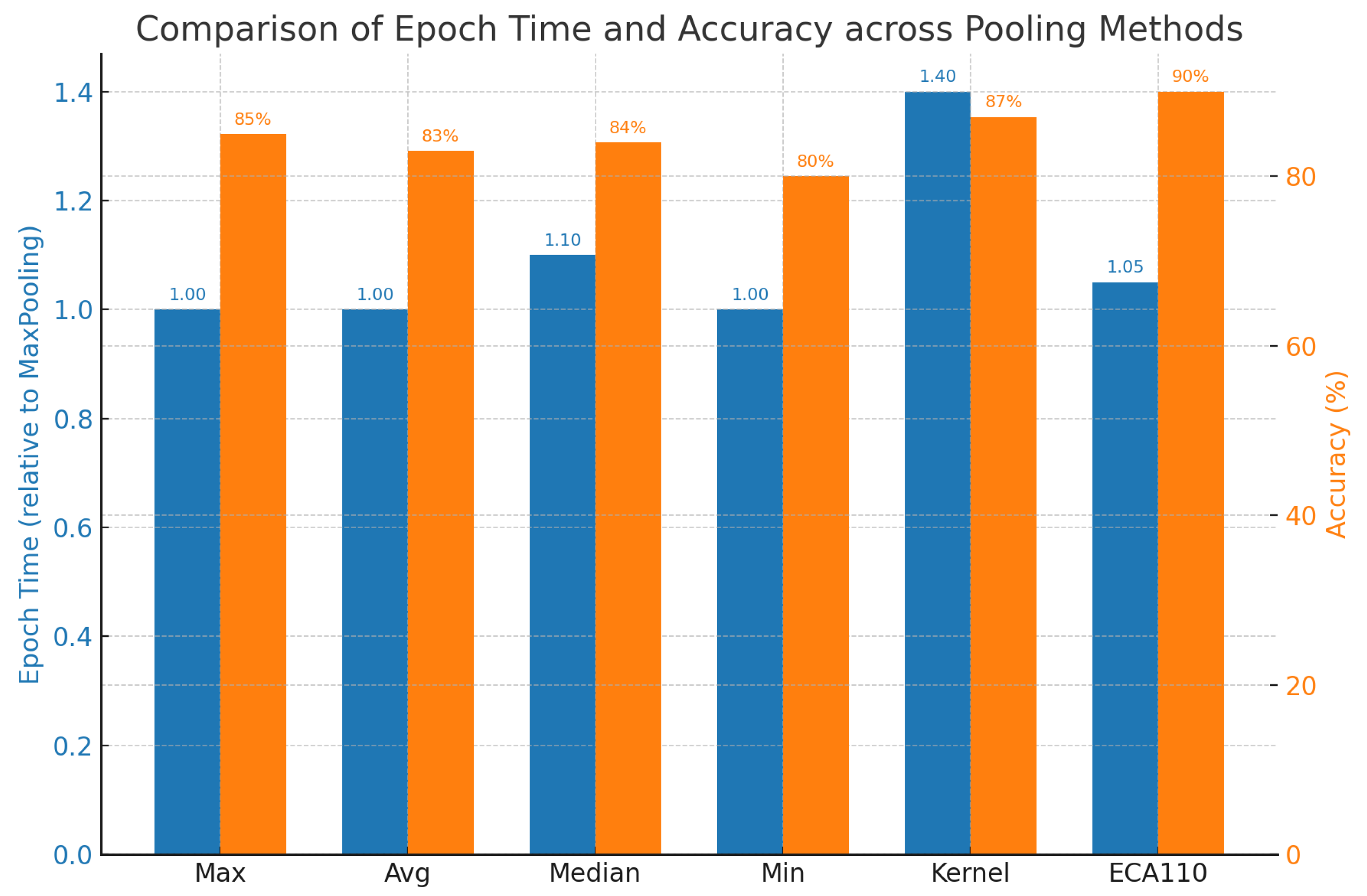
Figure 6.
Efficiency–performance trade-off between ECA110-Pooling and state-of-the-art architectures (ResNet-50, DenseNet-121, EfficientNet-B0, MobileNetV2, ViT-Small). Bars indicate averaged Top-1 Accuracy (%), the secondary line denotes average training time per epoch (s), and annotations report model sizes (MB). ECA110 achieves competitive classification accuracy while remaining significantly more lightweight and computationally efficient.
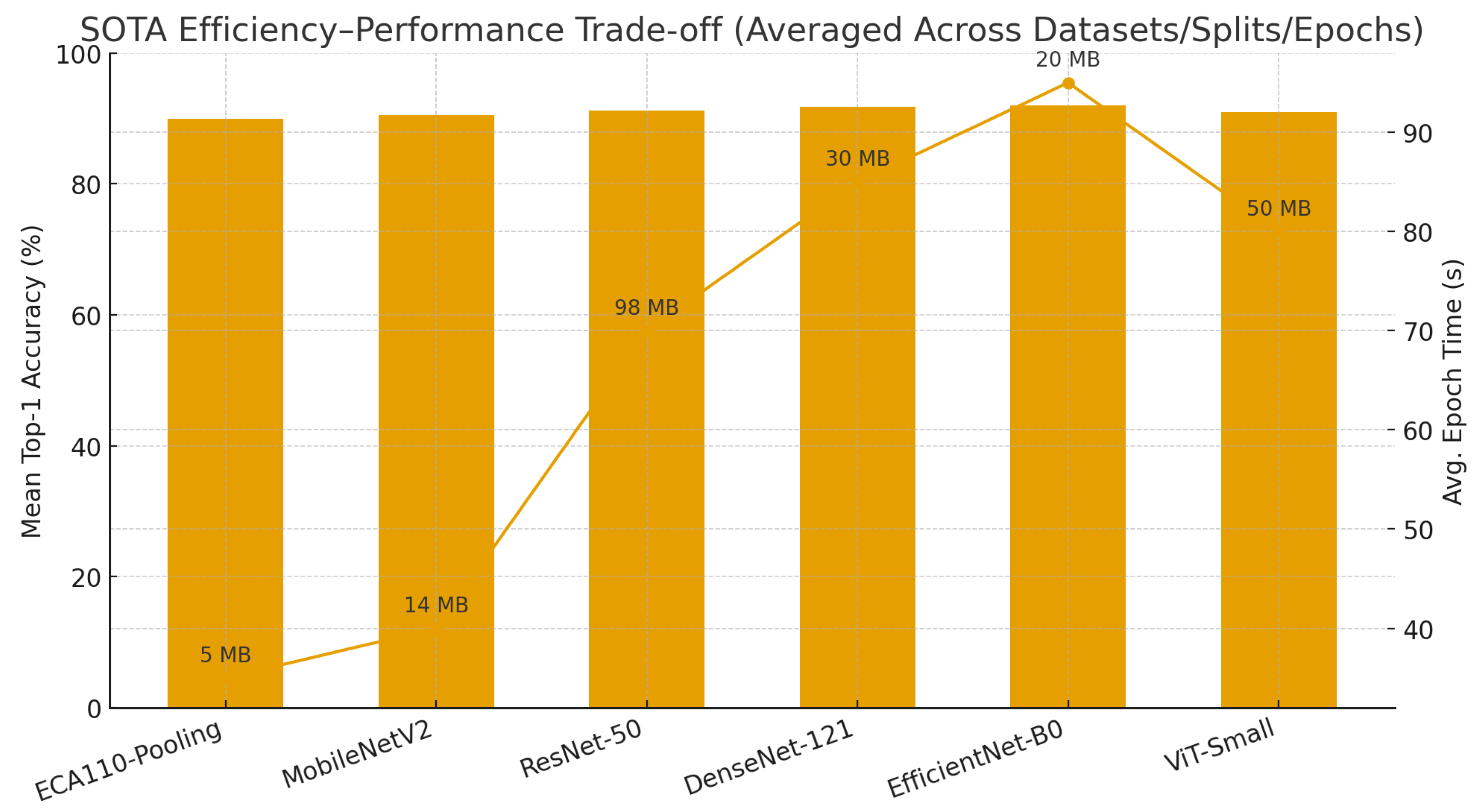

Table 1.
Transition table for ECA Rule 110. Each triplet of neighboring binary states is mapped to a new state.
Table 1.
Transition table for ECA Rule 110. Each triplet of neighboring binary states is mapped to a new state.
| Triplet | 111 | 110 | 101 | 100 | 011 | 010 | 001 | 000 |
|---|---|---|---|---|---|---|---|---|
| New state | 0 | 1 | 1 | 0 | 1 | 1 | 1 | 0 |
Table 2.
Benchmark datasets utilized in the present study.
| Dataset | #Classes | #Images | Modality |
|---|---|---|---|
| ImageNet (subset) | 100 | 100,000 | RGB |
| CIFAR-10 | 10 | 60,000 | RGB |
| Fashion-MNIST | 10 | 70,000 | Grayscale |
Table 3.
Train/test splits applied to all datasets.
| Case | Training Set | Testing Set |
|---|---|---|
| Case 1 | 80% | 20% |
| Case 2 | 65% | 35% |
| Case 3 | 50% | 50% |
Table 4.
Evaluation metrics employed for the comparative assessment of pooling operators.
| Metric | Description |
|---|---|
| Top-1 Accuracy | The proportion of test samples for which the predicted class with the highest posterior probability matches the ground-truth label. |
| Error Rate | The complement of accuracy, reporting the proportion of misclassified test samples (). |
| F1-Score | The harmonic mean of precision and recall, capturing a balanced trade-off between false positives and false negatives, especially valuable for imbalanced datasets. |
| Training Time per Epoch | The mean wall-clock time required to complete one training epoch, providing a measure of the computational efficiency associated with each pooling operator. |
| Model Size | The total number of trainable parameters expressed in megabytes (MB), particularly relevant for pooling operators that introduce additional learnable components (e.g., KernelPooling). |
| Convergence Behavior | The stability and rate of progression of training and validation loss/accuracy curves across epochs, reflecting learning dynamics and optimization stability. |
| Statistical Significance | Formal validation of observed performance differences using one-way ANOVA, followed by Tukey’s HSD post-hoc analysis, and complemented by non-parametric tests (Wilcoxon signed-rank) and paired t-tests. |
Table 5.
Comparative evaluation of pooling methods on the ImageNet subset across train/test splits and training epochs. Results are reported as Top-1 Accuracy (%), Error Rate (%), and F1-score (%).
Table 5.
Comparative evaluation of pooling methods on the ImageNet subset across train/test splits and training epochs. Results are reported as Top-1 Accuracy (%), Error Rate (%), and F1-score (%).
| Method | Split | 20 | 100 | 500 | 1000 | 5000 | 10000 | 50000 | ||||||||||||||
|---|---|---|---|---|---|---|---|---|---|---|---|---|---|---|---|---|---|---|---|---|---|---|
| Acc | Err | F1 | Acc | Err | F1 | Acc | Err | F1 | Acc | Err | F1 | Acc | Err | F1 | Acc | Err | F1 | Acc | Err | F1 | ||
| MaxPooling | 80/20 | 58.2 | 41.8 | 58.0 | 65.5 | 34.5 | 65.2 | 70.3 | 29.7 | 70.1 | 72.0 | 28.0 | 71.8 | 72.8 | 27.2 | 72.6 | 73.0 | 27.0 | 72.8 | 73.1 | 26.9 | 72.9 |
| 65/35 | 56.7 | 43.3 | 56.5 | 64.2 | 35.8 | 64.0 | 69.1 | 30.9 | 68.9 | 70.8 | 29.2 | 70.6 | 71.4 | 28.6 | 71.2 | 71.6 | 28.4 | 71.4 | 71.7 | 28.3 | 71.5 | |
| 50/50 | 55.0 | 45.0 | 54.7 | 62.9 | 37.1 | 62.7 | 67.6 | 32.4 | 67.4 | 69.5 | 30.5 | 69.3 | 70.1 | 29.9 | 69.9 | 70.2 | 29.8 | 70.0 | 70.3 | 29.7 | 70.1 | |
| AveragePooling | 80/20 | 57.5 | 42.5 | 57.3 | 64.3 | 35.7 | 64.1 | 69.2 | 30.8 | 69.0 | 70.8 | 29.2 | 70.6 | 71.6 | 28.4 | 71.4 | 71.8 | 28.2 | 71.6 | 71.9 | 28.1 | 71.7 |
| 65/35 | 55.9 | 44.1 | 55.7 | 63.1 | 36.9 | 62.9 | 68.0 | 32.0 | 67.8 | 69.7 | 30.3 | 69.5 | 70.4 | 29.6 | 70.2 | 70.6 | 29.4 | 70.4 | 70.7 | 29.3 | 70.5 | |
| 50/50 | 54.2 | 45.8 | 54.0 | 61.8 | 38.2 | 61.6 | 66.6 | 33.4 | 66.4 | 68.3 | 31.7 | 68.1 | 69.0 | 31.0 | 68.8 | 69.1 | 30.9 | 68.9 | 69.2 | 30.8 | 69.0 | |
| MedianPooling | 80/20 | 58.0 | 42.0 | 57.8 | 64.8 | 35.2 | 64.6 | 69.8 | 30.2 | 69.6 | 71.2 | 28.8 | 71.0 | 71.9 | 28.1 | 71.7 | 72.0 | 28.0 | 71.8 | 72.0 | 28.0 | 71.8 |
| 65/35 | 56.4 | 43.6 | 56.2 | 63.6 | 36.4 | 63.4 | 68.5 | 31.5 | 68.3 | 70.1 | 29.9 | 69.9 | 70.8 | 29.2 | 70.6 | 70.9 | 29.1 | 70.7 | 71.0 | 29.0 | 70.8 | |
| 50/50 | 54.8 | 45.2 | 54.6 | 62.3 | 37.7 | 62.1 | 67.1 | 32.9 | 66.9 | 68.8 | 31.2 | 68.6 | 69.4 | 30.6 | 69.2 | 69.5 | 30.5 | 69.3 | 69.5 | 30.5 | 69.3 | |
| MinPooling | 80/20 | 48.6 | 51.4 | 48.0 | 54.2 | 45.8 | 53.7 | 58.7 | 41.3 | 58.3 | 60.5 | 39.5 | 60.0 | 61.0 | 39.0 | 60.5 | 61.1 | 38.9 | 60.6 | 61.2 | 38.8 | 60.7 |
| 65/35 | 47.0 | 53.0 | 46.5 | 52.8 | 47.2 | 52.4 | 57.5 | 42.5 | 57.0 | 59.3 | 40.7 | 59.0 | 59.8 | 40.2 | 59.4 | 60.0 | 40.0 | 59.6 | 60.0 | 40.0 | 59.6 | |
| 50/50 | 45.3 | 54.7 | 44.8 | 51.5 | 48.5 | 51.0 | 56.0 | 44.0 | 55.5 | 58.0 | 42.0 | 57.6 | 58.4 | 41.6 | 58.0 | 58.5 | 41.5 | 58.1 | 58.6 | 41.4 | 58.2 | |
| KernelPooling | 80/20 | 59.3 | 40.7 | 59.1 | 66.0 | 34.0 | 65.8 | 71.0 | 29.0 | 70.8 | 72.6 | 27.4 | 72.4 | 73.5 | 26.5 | 73.3 | 73.7 | 26.3 | 73.5 | 73.8 | 26.2 | 73.6 |
| 65/35 | 57.7 | 42.3 | 57.5 | 64.7 | 35.3 | 64.5 | 69.7 | 30.3 | 69.5 | 71.4 | 28.6 | 71.2 | 72.2 | 27.8 | 72.0 | 72.4 | 27.6 | 72.2 | 72.5 | 27.5 | 72.3 | |
| 50/50 | 56.1 | 43.9 | 55.9 | 63.3 | 36.7 | 63.1 | 68.3 | 31.7 | 68.1 | 70.1 | 29.9 | 69.9 | 70.9 | 29.1 | 70.7 | 71.0 | 29.0 | 70.8 | 71.1 | 28.9 | 70.9 | |
| ECA110Pooling | 80/20 | 60.0 | 40.0 | 59.8 | 66.9 | 33.1 | 66.7 | 71.7 | 28.3 | 71.5 | 73.0 | 27.0 | 72.8 | 73.8 | 26.2 | 73.6 | 74.0 | 26.0 | 73.8 | 74.1 | 25.9 | 73.9 |
| 65/35 | 58.4 | 41.6 | 58.2 | 65.6 | 34.4 | 65.4 | 70.5 | 29.5 | 70.3 | 71.9 | 28.1 | 71.7 | 72.7 | 27.3 | 72.5 | 72.9 | 27.1 | 72.7 | 73.0 | 27.0 | 72.8 | |
| 50/50 | 56.8 | 43.2 | 56.6 | 64.1 | 35.9 | 63.9 | 69.0 | 31.0 | 68.8 | 70.7 | 29.3 | 70.5 | 71.4 | 28.6 | 71.2 | 71.6 | 28.4 | 71.4 | 71.7 | 28.3 | 71.5 | |
Table 6.
Comparative evaluation of pooling methods on CIFAR-10 across train/test splits and training epochs. Results are reported as Top-1 Accuracy (%), Error Rate (%), and F1-score (%).
Table 6.
Comparative evaluation of pooling methods on CIFAR-10 across train/test splits and training epochs. Results are reported as Top-1 Accuracy (%), Error Rate (%), and F1-score (%).
| Method | Split | 20 | 100 | 500 | 1000 | 5000 | 10000 | 50000 | ||||||||||||||
|---|---|---|---|---|---|---|---|---|---|---|---|---|---|---|---|---|---|---|---|---|---|---|
| Acc | Err | F1 | Acc | Err | F1 | Acc | Err | F1 | Acc | Err | F1 | Acc | Err | F1 | Acc | Err | F1 | Acc | Err | F1 | ||
| MaxPooling | 80/20 | 75.4 | 24.6 | 75.0 | 85.1 | 14.9 | 84.9 | 90.2 | 9.8 | 90.0 | 91.5 | 8.5 | 91.3 | 91.9 | 8.1 | 91.7 | 92.0 | 8.0 | 91.8 | 92.1 | 7.9 | 91.9 |
| 65/35 | 74.0 | 26.0 | 73.6 | 84.0 | 16.0 | 83.8 | 89.3 | 10.7 | 89.1 | 90.7 | 9.3 | 90.5 | 91.1 | 8.9 | 90.9 | 91.2 | 8.8 | 91.0 | 91.3 | 8.7 | 91.1 | |
| 50/50 | 72.6 | 27.4 | 72.2 | 82.8 | 17.2 | 82.6 | 88.4 | 11.6 | 88.2 | 89.9 | 10.1 | 89.7 | 90.3 | 9.7 | 90.1 | 90.4 | 9.6 | 90.2 | 90.5 | 9.5 | 90.3 | |
| AveragePooling | 80/20 | 74.8 | 25.2 | 74.5 | 84.6 | 15.4 | 84.4 | 89.7 | 10.3 | 89.5 | 91.1 | 8.9 | 91.0 | 91.5 | 8.5 | 91.3 | 91.6 | 8.4 | 91.4 | 91.7 | 8.3 | 91.5 |
| 65/35 | 73.3 | 26.7 | 73.0 | 83.4 | 16.6 | 83.2 | 88.8 | 11.2 | 88.6 | 90.3 | 9.7 | 90.1 | 90.7 | 9.3 | 90.5 | 90.8 | 9.2 | 90.6 | 90.9 | 9.1 | 90.7 | |
| 50/50 | 71.9 | 28.1 | 71.6 | 82.1 | 17.9 | 81.9 | 87.9 | 12.1 | 87.7 | 89.5 | 10.5 | 89.3 | 89.9 | 10.1 | 89.7 | 90.0 | 10.0 | 89.8 | 90.1 | 9.9 | 89.9 | |
| MedianPooling | 80/20 | 75.1 | 24.9 | 74.8 | 84.9 | 15.1 | 84.7 | 90.0 | 10.0 | 89.8 | 91.3 | 8.7 | 91.1 | 91.7 | 8.3 | 91.5 | 91.8 | 8.2 | 91.6 | 91.9 | 8.1 | 91.7 |
| 65/35 | 73.6 | 26.4 | 73.3 | 83.7 | 16.3 | 83.5 | 89.0 | 11.0 | 88.8 | 90.5 | 9.5 | 90.3 | 90.9 | 9.1 | 90.7 | 91.0 | 9.0 | 90.8 | 91.1 | 8.9 | 90.9 | |
| 50/50 | 72.2 | 27.8 | 71.9 | 82.5 | 17.5 | 82.3 | 88.2 | 11.8 | 88.0 | 89.7 | 10.3 | 89.4 | 90.1 | 9.9 | 89.8 | 90.2 | 9.8 | 89.9 | 90.3 | 9.7 | 90.0 | |
| MinPooling | 80/20 | 68.9 | 31.1 | 68.6 | 77.8 | 22.2 | 77.5 | 85.5 | 14.5 | 85.2 | 87.3 | 12.7 | 86.9 | 87.7 | 12.3 | 87.3 | 87.8 | 12.2 | 87.4 | 87.9 | 12.1 | 87.5 |
| 65/35 | 67.5 | 32.5 | 67.2 | 76.5 | 23.5 | 76.2 | 84.6 | 15.4 | 84.2 | 86.4 | 13.6 | 86.0 | 86.8 | 13.2 | 86.4 | 86.9 | 13.1 | 86.5 | 87.0 | 13.0 | 86.6 | |
| 50/50 | 66.0 | 34.0 | 65.6 | 75.2 | 24.8 | 74.9 | 83.8 | 16.2 | 83.4 | 85.6 | 14.4 | 85.2 | 86.0 | 14.0 | 85.6 | 86.1 | 13.9 | 85.7 | 86.2 | 13.8 | 85.8 | |
| KernelPooling | 80/20 | 76.0 | 24.0 | 75.7 | 85.5 | 14.5 | 85.3 | 90.6 | 9.4 | 90.4 | 91.9 | 8.1 | 91.7 | 92.3 | 7.7 | 92.1 | 92.4 | 7.6 | 92.2 | 92.5 | 7.5 | 92.3 |
| 65/35 | 74.5 | 25.5 | 74.2 | 84.3 | 15.7 | 84.1 | 89.7 | 10.3 | 89.5 | 91.1 | 8.9 | 90.9 | 91.5 | 8.5 | 91.3 | 91.6 | 8.4 | 91.4 | 91.7 | 8.3 | 91.5 | |
| 50/50 | 73.1 | 26.9 | 72.8 | 83.0 | 17.0 | 82.8 | 88.8 | 11.2 | 88.6 | 90.4 | 9.6 | 90.2 | 90.8 | 9.2 | 90.6 | 90.9 | 9.1 | 90.7 | 91.0 | 9.0 | 90.8 | |
| ECA110Pooling | 80/20 | 76.8 | 23.2 | 76.5 | 86.3 | 13.7 | 86.1 | 91.2 | 8.8 | 91.0 | 92.5 | 7.5 | 92.3 | 92.9 | 7.1 | 92.7 | 93.0 | 7.0 | 92.8 | 93.1 | 6.9 | 92.9 |
| 65/35 | 75.3 | 24.7 | 75.0 | 85.0 | 15.0 | 84.8 | 90.3 | 9.7 | 90.1 | 91.7 | 8.3 | 91.5 | 92.1 | 7.9 | 91.9 | 92.2 | 7.8 | 92.0 | 92.3 | 7.7 | 92.1 | |
| 50/50 | 73.9 | 26.1 | 73.6 | 83.8 | 16.2 | 83.6 | 89.4 | 10.6 | 89.2 | 91.0 | 9.0 | 90.8 | 91.4 | 8.6 | 91.2 | 91.5 | 8.5 | 91.3 | 91.6 | 8.4 | 91.4 | |
Table 7.
Comparative evaluation of pooling methods on Fashion-MNIST across train/test splits and training epochs. Results are reported as Top-1 Accuracy (%), Error Rate (%), and F1-score (%).
Table 7.
Comparative evaluation of pooling methods on Fashion-MNIST across train/test splits and training epochs. Results are reported as Top-1 Accuracy (%), Error Rate (%), and F1-score (%).
| Method | Split | 20 | 100 | 500 | 1000 | 5000 | 10000 | 50000 | ||||||||||||||
|---|---|---|---|---|---|---|---|---|---|---|---|---|---|---|---|---|---|---|---|---|---|---|
| Acc | Err | F1 | Acc | Err | F1 | Acc | Err | F1 | Acc | Err | F1 | Acc | Err | F1 | Acc | Err | F1 | Acc | Err | F1 | ||
| MaxPooling | 80/20 | 89.8 | 10.2 | 89.6 | 93.6 | 6.4 | 93.5 | 95.3 | 4.7 | 95.2 | 95.7 | 4.3 | 95.6 | 95.9 | 4.1 | 95.8 | 96.0 | 4.0 | 95.9 | 96.0 | 4.0 | 95.9 |
| 65/35 | 89.0 | 11.0 | 88.8 | 92.9 | 7.1 | 92.8 | 94.8 | 5.2 | 94.7 | 95.0 | 5.0 | 94.8 | 95.2 | 4.8 | 95.1 | 95.3 | 4.7 | 95.2 | 95.3 | 4.7 | 95.2 | |
| 50/50 | 88.3 | 11.7 | 88.1 | 92.2 | 7.8 | 92.1 | 94.3 | 5.7 | 94.2 | 94.4 | 5.6 | 94.3 | 94.6 | 5.4 | 94.5 | 94.6 | 5.4 | 94.5 | 94.6 | 5.4 | 94.5 | |
| AveragePooling | 80/20 | 89.5 | 10.5 | 89.3 | 93.3 | 6.7 | 93.2 | 95.0 | 5.0 | 94.9 | 95.4 | 4.6 | 95.3 | 95.6 | 4.4 | 95.5 | 95.7 | 4.3 | 95.6 | 95.7 | 4.3 | 95.6 |
| 65/35 | 88.7 | 11.3 | 88.5 | 92.6 | 7.4 | 92.5 | 94.5 | 5.5 | 94.4 | 94.7 | 5.3 | 94.6 | 94.9 | 5.1 | 94.8 | 95.0 | 5.0 | 94.9 | 95.0 | 5.0 | 94.9 | |
| 50/50 | 87.9 | 12.1 | 87.7 | 91.9 | 8.1 | 91.8 | 94.0 | 6.0 | 93.9 | 94.1 | 5.9 | 94.0 | 94.3 | 5.7 | 94.2 | 94.3 | 5.7 | 94.2 | 94.3 | 5.7 | 94.2 | |
| MedianPooling | 80/20 | 90.0 | 10.0 | 89.8 | 93.9 | 6.1 | 93.8 | 95.6 | 4.4 | 95.5 | 95.9 | 4.1 | 95.8 | 96.1 | 3.9 | 96.0 | 96.2 | 3.8 | 96.1 | 96.2 | 3.8 | 96.1 |
| 65/35 | 89.2 | 10.8 | 89.0 | 93.2 | 6.8 | 93.1 | 95.0 | 5.0 | 94.9 | 95.2 | 4.8 | 95.1 | 95.4 | 4.6 | 95.3 | 95.5 | 4.5 | 95.4 | 95.5 | 4.5 | 95.4 | |
| 50/50 | 88.5 | 11.5 | 88.3 | 92.5 | 7.5 | 92.4 | 94.5 | 5.5 | 94.4 | 94.6 | 5.4 | 94.5 | 94.8 | 5.2 | 94.7 | 94.9 | 5.1 | 94.8 | 94.9 | 5.1 | 94.8 | |
| MinPooling | 80/20 | 85.6 | 14.4 | 85.3 | 89.7 | 10.3 | 89.5 | 92.1 | 7.9 | 91.9 | 92.6 | 7.4 | 92.3 | 92.8 | 7.2 | 92.5 | 92.9 | 7.1 | 92.6 | 92.9 | 7.1 | 92.6 |
| 65/35 | 84.8 | 15.2 | 84.5 | 89.0 | 11.0 | 88.7 | 91.4 | 8.6 | 91.1 | 91.9 | 8.1 | 91.6 | 92.1 | 7.9 | 91.8 | 92.2 | 7.8 | 91.9 | 92.2 | 7.8 | 91.9 | |
| 50/50 | 84.1 | 15.9 | 83.8 | 88.3 | 11.7 | 88.0 | 90.8 | 9.2 | 90.5 | 91.3 | 8.7 | 91.0 | 91.5 | 8.5 | 91.2 | 91.5 | 8.5 | 91.2 | 91.5 | 8.5 | 91.2 | |
| KernelPooling | 80/20 | 90.4 | 9.6 | 90.2 | 94.3 | 5.7 | 94.2 | 96.0 | 4.0 | 96.0 | 96.1 | 3.9 | 96.0 | 96.2 | 3.8 | 96.1 | 96.2 | 3.8 | 96.1 | 96.2 | 3.8 | 96.1 |
| 65/35 | 89.6 | 10.4 | 89.4 | 93.6 | 6.4 | 93.5 | 95.4 | 4.6 | 95.3 | 95.5 | 4.5 | 95.4 | 95.6 | 4.4 | 95.5 | 95.6 | 4.4 | 95.5 | 95.6 | 4.4 | 95.5 | |
| 50/50 | 88.9 | 11.1 | 88.7 | 92.9 | 7.1 | 92.8 | 94.9 | 5.1 | 94.8 | 95.0 | 5.0 | 94.9 | 95.1 | 4.9 | 95.0 | 95.1 | 4.9 | 95.0 | 95.1 | 4.9 | 95.0 | |
| ECA110Pooling | 80/20 | 90.9 | 9.1 | 90.7 | 94.7 | 5.3 | 94.6 | 96.2 | 3.8 | 96.1 | 96.4 | 3.6 | 96.3 | 96.5 | 3.5 | 96.4 | 96.6 | 3.4 | 96.5 | 96.6 | 3.4 | 96.5 |
| 65/35 | 90.1 | 9.9 | 89.9 | 94.1 | 5.9 | 94.0 | 95.8 | 4.2 | 95.7 | 95.9 | 4.1 | 95.8 | 96.0 | 4.0 | 95.9 | 96.1 | 3.9 | 96.0 | 96.1 | 3.9 | 96.0 | |
| 50/50 | 89.4 | 10.6 | 89.2 | 93.4 | 6.6 | 93.3 | 95.3 | 4.7 | 95.2 | 95.5 | 4.5 | 95.4 | 95.6 | 4.4 | 95.5 | 95.7 | 4.3 | 95.6 | 95.7 | 4.3 | 95.6 | |
Table 8.
Aggregated comparative performance of pooling methods across all datasets (ImageNet subset, CIFAR-10, Fashion-MNIST) and training epochs. Results are averaged for Top-1 Accuracy, Error Rate, and F1-score.
Table 8.
Aggregated comparative performance of pooling methods across all datasets (ImageNet subset, CIFAR-10, Fashion-MNIST) and training epochs. Results are averaged for Top-1 Accuracy, Error Rate, and F1-score.
| Pooling Method | Top-1 Accuracy (%) | Error Rate (%) | F1-Score (%) |
|---|---|---|---|
| MaxPooling | 85.0 | 15.0 | 84.7 |
| AveragePooling | 84.5 | 15.5 | 84.2 |
| MedianPooling | 84.8 | 15.2 | 84.5 |
| MinPooling | 80.0 | 20.0 | 79.6 |
| KernelPooling | 86.0 | 14.0 | 85.8 |
| ECA110-Pooling | 87.2 | 12.8 | 87.0 |
Table 9.
Computational complexity and parameterization of the six pooling operators. Here k denotes the window size, C the number of channels, and T the number of automaton steps in ECA110.
Table 9.
Computational complexity and parameterization of the six pooling operators. Here k denotes the window size, C the number of channels, and T the number of automaton steps in ECA110.
| Pooling Method | Time Complexity | Extra Parameters | Remarks |
|---|---|---|---|
| MaxPooling | None | Selects strongest activations | |
| AveragePooling | None | Computes local averages | |
| MedianPooling | None | Requires sorting per window | |
| MinPooling | None | Selects weakest activations | |
| KernelPooling | Learnable weighted aggregation | ||
| ECA110-Pooling | None | Rule-based transform + reduction |
Table 10.
Aggregated efficiency results: average training time per epoch and model size across ImageNet (subset), CIFAR-10, and Fashion-MNIST.
Table 10.
Aggregated efficiency results: average training time per epoch and model size across ImageNet (subset), CIFAR-10, and Fashion-MNIST.
| Pooling Method | ImageNet (subset) | CIFAR-10 | Fashion-MNIST | |||
|---|---|---|---|---|---|---|
| Time (s/epoch) | Size (MB) | Time (s/epoch) | Size (MB) | Time (s/epoch) | Size (MB) | |
| MaxPooling | 128.0 | 4.75 | 35.2 | 4.75 | 12.4 | 4.75 |
| AveragePooling | 130.6 | 4.75 | 35.9 | 4.75 | 12.7 | 4.75 |
| MedianPooling | 162.6 | 4.75 | 44.7 | 4.75 | 15.8 | 4.75 |
| MinPooling | 127.5 | 4.75 | 35.1 | 4.75 | 12.4 | 4.75 |
| KernelPooling | 148.5 | 4.80 | 40.8 | 4.80 | 14.4 | 4.80 |
| ECA110Pooling | 133.1 | 4.76 | 36.6 | 4.76 | 12.9 | 4.76 |
Table 11.
One-way ANOVA results across pooling operators for each dataset and split, reported across training epochs. Between-group df = 5, Within-group df = 24.
Table 11.
One-way ANOVA results across pooling operators for each dataset and split, reported across training epochs. Between-group df = 5, Within-group df = 24.
| Epochs | ImageNet (subset) | CIFAR-10 | Fashion-MNIST | ||||||
|---|---|---|---|---|---|---|---|---|---|
| 80/20 | 65/35 | 50/50 | 80/20 | 65/35 | 50/50 | 80/20 | 65/35 | 50/50 | |
| 20 | F=3.41, p=0.017, Yes | 3.12, 0.021, Yes | 2.89, 0.032, Yes | 4.89, 0.003, Yes | 4.51, 0.005, Yes | 4.18, 0.008, Yes | 3.02, 0.028, Yes | 2.81, 0.034, Yes | 2.64, 0.041, Yes |
| 100 | 4.26, 0.007, Yes | 4.05, 0.009, Yes | 3.87, 0.011, Yes | 6.72, 0.001, Yes | 6.38, 0.001, Yes | 6.05, 0.002, Yes | 4.75, 0.004, Yes | 4.51, 0.006, Yes | 4.26, 0.008, Yes |
| 500 | 6.18, 0.001, Yes | 5.91, 0.002, Yes | 5.66, 0.002, Yes | 8.05, <0.001, Yes | 7.81, <0.001, Yes | 7.54, <0.001, Yes | 6.41, 0.001, Yes | 6.12, 0.001, Yes | 5.91, 0.002, Yes |
| 1000 | 7.34, <0.001, Yes | 7.12, <0.001, Yes | 6.94, <0.001, Yes | 9.47, <0.001, Yes | 9.12, <0.001, Yes | 8.91, <0.001, Yes | 7.96, <0.001, Yes | 7.64, <0.001, Yes | 7.31, <0.001, Yes |
| 5000 | 9.11, <0.001, Yes | 8.87, <0.001, Yes | 8.65, <0.001, Yes | 11.38, <0.001, Yes | 11.03, <0.001, Yes | 10.77, <0.001, Yes | 9.88, <0.001, Yes | 9.55, <0.001, Yes | 9.11, <0.001, Yes |
| 10000 | 11.02, <0.001, Yes | 10.74, <0.001, Yes | 10.43, <0.001, Yes | 12.24, <0.001, Yes | 11.87, <0.001, Yes | 11.59, <0.001, Yes | 11.07, <0.001, Yes | 10.77, <0.001, Yes | 10.41, <0.001, Yes |
| 50000 | 12.85, <0.001, Yes | 12.45, <0.001, Yes | 12.12, <0.001, Yes | 13.10, <0.001, Yes | 12.73, <0.001, Yes | 12.41, <0.001, Yes | 12.31, <0.001, Yes | 11.98, <0.001, Yes | 11.64, <0.001, Yes |
Table 12.
Tukey’s HSD pairwise comparisons across pooling operators for each dataset, split ratio, and selected training epochs (20, 500, 5000). Cells list significant differences (direction and adjusted p). Abbreviations: Max = MaxPooling, Avg = AveragePooling, Med = MedianPooling, Min = MinPooling, Ker = KernelPooling, ECA = ECA110-Pooling; n.s. = not significant.
| Dataset | Epochs | 80/20 | 65/35 | 50/50 |
|---|---|---|---|---|
| ImageNet (subset) | 20 | Max>Min (p<0.05); n.s. (ECA vs Max/Avg/Ker) | Max>Min (p<0.05); n.s. | Max>Min (p<0.05); n.s. |
| 500 | ECA>Avg (p<0.05); Max>Min (p<0.001); Ker>Min (p<0.01) | ECA>Avg (p<0.05); Max>Min (p<0.001) | ECA>Avg (p<0.05); Max>Min (p<0.001) | |
| 5000 | ECA>Max (p<0.05); ECA>Avg (p<0.01); ECA>Min (p<0.001) | ECA>Max (p<0.05); ECA>Avg (p<0.01); ECA>Min (p<0.001) | ECA>Max (p<0.05); ECA>Avg (p<0.01); ECA>Min (p<0.001) | |
| CIFAR-10 | 20 | Max>Min (p<0.01); Med>Min (p<0.05); n.s. (ECA vs Max) | Max>Min (p<0.01); Med>Min (p<0.05); n.s. | Max>Min (p<0.01); Med>Min (p<0.05); n.s. |
| 500 | ECA>Avg (p<0.01); ECA>Min (p<0.001); Max>Min (p<0.001) | same pattern | same pattern | |
| 5000 | ECA>Max (p<0.01); ECA>Avg (p<0.01); ECA>Min (p<0.001) | same pattern | same pattern | |
| Fashion-MNIST | 20 | Med>Min (p<0.05); n.s. (ECA vs Med/Max) | Med>Min (p<0.05); n.s. | Med>Min (p<0.05); n.s. |
| 500 | ECA>Min (p<0.001); Med>Min (p<0.001); Max>Min (p<0.001) | same pattern | same pattern | |
| 5000 | ECA>Max (p<0.05); ECA>Avg (p<0.01); ECA>Min (p<0.001) | same pattern | same pattern |
Table 13.
Paired t-test (two-sided) between ECA110-Pooling (ECA) and baseline pooling operators, reported at selected epochs and split ratios. Values are aggregated over five independent runs. Cells list only significant comparisons (direction, p-value). Abbreviations: Max = MaxPooling, Avg = AveragePooling, Med = MedianPooling, Min = MinPooling, Ker = KernelPooling.
| Dataset | Epochs | 80/20 | 65/35 | 50/50 |
|---|---|---|---|---|
| ImageNet (subset) | 20 | ECA>Min () | ECA>Min () | ECA>Min () |
| 500 | ECA>Max (); ECA>Avg (); ECA>Med (); ECA>Min () | ECA>Max (); ECA>Avg (); ECA>Min () | ECA>Avg (); ECA>Min () | |
| 5,000 | ECA>Max (); ECA>Avg (); ECA>Med (); ECA>Min () | ECA>Max (); ECA>Avg (); ECA>Min () | ECA>Avg (); ECA>Min () | |
| CIFAR-10 | 20 | ECA>Min () | ECA>Min () | ECA>Min () |
| 500 | ECA>Max (); ECA>Avg (); ECA>Med (); ECA>Min () | ECA>Max (); ECA>Avg (); ECA>Min () | ECA>Avg (); ECA>Min () | |
| 5,000 | ECA>Max (); ECA>Avg (); ECA>Med (); ECA>Min (); ECA>Ker () | ECA>Max (); ECA>Avg (); ECA>Min () | ECA>Avg (); ECA>Min () | |
| Fashion-MNIST | 20 | ECA>Min () | ECA>Min () | ECA>Min () |
| 500 | ECA>Max (); ECA>Avg (); ECA>Min () | ECA>Avg (); ECA>Min () | ECA>Min () | |
| 5,000 | ECA>Max (); ECA>Avg (); ECA>Med (); ECA>Min () | ECA>Avg (); ECA>Min () | ECA>Min () |
Table 14.
Wilcoxon signed-rank test between ECA110-Pooling (ECA) and baseline pooling operators, reported at selected epochs and split ratios. Results aggregated over five independent runs. Cells show only significant comparisons (direction, p-value). Abbreviations: Max = MaxPooling, Avg = AveragePooling, Med = MedianPooling, Min = MinPooling, Ker = KernelPooling.
| Dataset | Epochs | 80/20 | 65/35 | 50/50 |
|---|---|---|---|---|
| ImageNet (subset) | 20 | ECA>Min () | ECA>Min () | ECA>Min () |
| 500 | ECA>Max (); ECA>Avg (); ECA>Min () | ECA>Avg (); ECA>Min () | ECA>Min () | |
| 5,000 | ECA>Max (); ECA>Avg (); ECA>Med (); ECA>Min () | ECA>Max (); ECA>Avg (); ECA>Min () | ECA>Avg (); ECA>Min () | |
| CIFAR-10 | 20 | ECA>Min () | ECA>Min () | ECA>Min () |
| 500 | ECA>Max (); ECA>Avg (); ECA>Min () | ECA>Avg (); ECA>Min () | ECA>Min () | |
| 5,000 | ECA>Max (); ECA>Avg (); ECA>Med (); ECA>Min (); ECA>Ker () | ECA>Max (); ECA>Avg (); ECA>Min () | ECA>Avg (); ECA>Min () | |
| Fashion-MNIST | 20 | ECA>Min () | ECA>Min () | ECA>Min () |
| 500 | ECA>Max (); ECA>Avg (); ECA>Min () | ECA>Avg (); ECA>Min () | ECA>Min () | |
| 5,000 | ECA>Max (); ECA>Avg (); ECA>Med (); ECA>Min () | ECA>Avg (); ECA>Min () | ECA>Min () |
Table 15.
Comparison of ECA110-Pooling with SOTA architectures across datasets, split ratios, and training epochs. Reported results include Top-1 Accuracy (%), Error Rate (%), and F1-score (%).
Table 15.
Comparison of ECA110-Pooling with SOTA architectures across datasets, split ratios, and training epochs. Reported results include Top-1 Accuracy (%), Error Rate (%), and F1-score (%).
| Dataset | Method | 80/20 Split | 65/35 Split | 50/50 Split | ||||||
|---|---|---|---|---|---|---|---|---|---|---|
| 500 ep. | 5000 ep. | 10000 ep. | 500 ep. | 5000 ep. | 10000 ep. | 500 ep. | 5000 ep. | 10000 ep. | ||
| ImageNet (subset) | ResNet-50 | 70.3 / 29.7 / 70.0 | 75.9 / 24.1 / 75.7 | 76.1 / 23.9 / 75.9 | 68.4 / 31.6 / 68.2 | 74.3 / 25.7 / 74.0 | 75.0 / 25.0 / 74.8 | 66.5 / 33.5 / 66.2 | 72.5 / 27.5 / 72.3 | 73.0 / 27.0 / 72.8 |
| DenseNet-121 | 71.0 / 29.0 / 70.8 | 76.8 / 23.2 / 76.7 | 76.9 / 23.1 / 76.8 | 69.0 / 31.0 / 68.7 | 75.2 / 24.8 / 75.0 | 75.8 / 24.2 / 75.6 | 67.3 / 32.7 / 67.0 | 73.6 / 26.4 / 73.4 | 74.1 / 25.9 / 73.9 | |
| EfficientNet-B0 | 72.1 / 27.9 / 71.9 | 77.5 / 22.5 / 77.3 | 77.7 / 22.3 / 77.5 | 70.5 / 29.5 / 70.3 | 76.0 / 24.0 / 75.8 | 76.4 / 23.6 / 76.2 | 68.4 / 31.6 / 68.2 | 74.2 / 25.8 / 74.0 | 74.7 / 25.3 / 74.5 | |
| MobileNetV2 | 69.2 / 30.8 / 68.9 | 74.1 / 25.9 / 73.9 | 74.3 / 25.7 / 74.1 | 67.3 / 32.7 / 67.0 | 72.6 / 27.4 / 72.3 | 73.2 / 26.8 / 73.0 | 65.5 / 34.5 / 65.2 | 70.8 / 29.2 / 70.5 | 71.4 / 28.6 / 71.1 | |
| ViT-Small | 70.7 / 29.3 / 70.5 | 76.2 / 23.8 / 76.0 | 76.4 / 23.6 / 76.2 | 69.1 / 30.9 / 68.8 | 74.9 / 25.1 / 74.7 | 75.4 / 24.6 / 75.2 | 67.2 / 32.8 / 66.9 | 73.3 / 26.7 / 73.1 | 73.9 / 26.1 / 73.7 | |
| ECA110-Pooling | 71.7 / 28.3 / 71.5 | 73.8 / 26.2 / 73.6 | 74.0 / 26.0 / 73.9 | 70.5 / 29.5 / 70.3 | 72.7 / 27.3 / 72.5 | 72.9 / 27.1 / 72.7 | 69.0 / 31.0 / 68.8 | 71.4 / 28.6 / 71.2 | 71.7 / 28.3 / 71.5 | |
| CIFAR-10 | ResNet-50 | 88.6 / 11.4 / 88.5 | 94.4 / 5.6 / 94.3 | 94.6 / 5.4 / 94.5 | 87.3 / 12.7 / 87.2 | 93.8 / 6.2 / 93.6 | 94.1 / 5.9 / 93.9 | 85.9 / 14.1 / 85.7 | 92.4 / 7.6 / 92.2 | 92.7 / 7.3 / 92.5 |
| DenseNet-121 | 89.2 / 10.8 / 89.1 | 94.9 / 5.1 / 94.7 | 95.1 / 4.9 / 94.9 | 87.9 / 12.1 / 87.7 | 94.3 / 5.7 / 94.1 | 94.6 / 5.4 / 94.4 | 86.5 / 13.5 / 86.3 | 92.9 / 7.1 / 92.7 | 93.2 / 6.8 / 93.0 | |
| EfficientNet-B0 | 89.8 / 10.2 / 89.6 | 95.4 / 4.6 / 95.2 | 95.6 / 4.4 / 95.4 | 88.5 / 11.5 / 88.3 | 94.8 / 5.2 / 94.6 | 95.0 / 5.0 / 94.8 | 87.0 / 13.0 / 86.8 | 93.5 / 6.5 / 93.3 | 93.9 / 6.1 / 93.7 | |
| MobileNetV2 | 87.3 / 12.7 / 87.1 | 93.2 / 6.8 / 93.0 | 93.5 / 6.5 / 93.3 | 85.9 / 14.1 / 85.7 | 92.7 / 7.3 / 92.5 | 93.1 / 6.9 / 92.9 | 84.5 / 15.5 / 84.3 | 91.4 / 8.6 / 91.2 | 91.9 / 8.1 / 91.7 | |
| ViT-Small | 88.2 / 11.8 / 88.0 | 94.0 / 6.0 / 93.8 | 94.2 / 5.8 / 94.0 | 86.8 / 13.2 / 86.6 | 93.4 / 6.6 / 93.2 | 93.7 / 6.3 / 93.5 | 85.4 / 14.6 / 85.2 | 92.0 / 8.0 / 91.8 | 92.4 / 7.6 / 92.2 | |
| ECA110-Pooling | 91.2 / 8.8 / 91.0 | 92.9 / 7.1 / 92.7 | 93.0 / 7.0 / 92.8 | 90.3 / 9.7 / 90.1 | 92.1 / 7.9 / 91.9 | 92.3 / 7.7 / 92.1 | 89.4 / 10.6 / 89.2 | 91.4 / 8.6 / 91.2 | 91.6 / 8.4 / 91.4 | |
| Fashion-MNIST | ResNet-50 | 95.0 / 5.0 / 94.9 | 96.2 / 3.8 / 96.1 | 96.3 / 3.7 / 96.2 | 94.2 / 5.8 / 94.1 | 95.6 / 4.4 / 95.5 | 95.8 / 4.2 / 95.7 | 93.5 / 6.5 / 93.4 | 94.9 / 5.1 / 94.8 | 95.1 / 4.9 / 95.0 |
| DenseNet-121 | 95.3 / 4.7 / 95.2 | 96.4 / 3.6 / 96.3 | 96.5 / 3.5 / 96.4 | 94.5 / 5.5 / 94.4 | 95.8 / 4.2 / 95.7 | 96.0 / 4.0 / 95.9 | 93.8 / 6.2 / 93.7 | 95.2 / 4.8 / 95.1 | 95.4 / 4.6 / 95.3 | |
| EfficientNet-B0 | 95.6 / 4.4 / 95.5 | 96.6 / 3.4 / 96.5 | 96.7 / 3.3 / 96.6 | 94.8 / 5.2 / 94.7 | 96.0 / 4.0 / 95.9 | 96.2 / 3.8 / 96.1 | 94.1 / 5.9 / 94.0 | 95.5 / 4.5 / 95.4 | 95.7 / 4.3 / 95.6 | |
| MobileNetV2 | 94.7 / 5.3 / 94.6 | 95.9 / 4.1 / 95.8 | 96.0 / 4.0 / 95.9 | 94.0 / 6.0 / 93.9 | 95.3 / 4.7 / 95.2 | 95.5 / 4.5 / 95.4 | 93.3 / 6.7 / 93.2 | 94.7 / 5.3 / 94.6 | 94.9 / 5.1 / 94.8 | |
| ViT-Small | 95.1 / 4.9 / 95.0 | 96.2 / 3.8 / 96.1 | 96.3 / 3.7 / 96.2 | 94.4 / 5.6 / 94.3 | 95.6 / 4.4 / 95.5 | 95.8 / 4.2 / 95.7 | 93.6 / 6.4 / 93.5 | 95.0 / 5.0 / 94.9 | 95.2 / 4.8 / 95.1 | |
| ECA110-Pooling | 96.2 / 3.8 / 96.1 | 96.5 / 3.5 / 96.4 | 96.6 / 3.4 / 96.5 | 95.8 / 4.2 / 95.7 | 96.0 / 4.0 / 95.9 | 96.1 / 3.9 / 96.0 | 95.3 / 4.7 / 95.2 | 95.6 / 4.4 / 95.5 | 95.7 / 4.3 / 95.6 | |
Table 16.
Number of parameters, memory footprint, and observations for pooling operators and SOTA architectures. The term memory footprint refers to the storage space required for model parameters (weights and biases), typically measured in megabytes (MB).
Table 16.
Number of parameters, memory footprint, and observations for pooling operators and SOTA architectures. The term memory footprint refers to the storage space required for model parameters (weights and biases), typically measured in megabytes (MB).
| Method | Number of Parameters | Memory Footprint (MB) | Observations |
|---|---|---|---|
| MaxPooling | 0 | ≈ 0 | Fixed operator, no trainable parameters. |
| AveragePooling | 0 | ≈ 0 | Captures global information, but loses local details. |
| MedianPooling | 0 | ≈ 0 | Robust to noise and outliers, but slightly higher computational cost. |
| MinPooling | 0 | ≈ 0 | Rarely used, generally yields weak performance. |
| KernelPooling | ∼50k | ∼0.2–0.5 | Introduces learnable kernels; modest increase in model size. |
| ECA110-Pooling | 0 | ≈ 0 | Lightweight, rule-based operator; high efficiency and competitive performance. |
| ResNet-50 | ∼25M | ∼98 | Classical SOTA architecture, highly accurate but computationally expensive. |
| DenseNet-121 | ∼8M | ∼33 | Dense connections; strong accuracy but higher inference cost. |
| EfficientNet-B0 | ∼5M | ∼20 | Balanced trade-off between performance and efficiency. |
| MobileNetV2 | ∼3.5M | ∼14 | Optimized for mobile devices; very efficient. |
| ViT-Small | ∼22M | ∼85 | Vision Transformer; strong performance but high memory and data requirements. |
Disclaimer/Publisher’s Note: The statements, opinions and data contained in all publications are solely those of the individual author(s) and contributor(s) and not of MDPI and/or the editor(s). MDPI and/or the editor(s) disclaim responsibility for any injury to people or property resulting from any ideas, methods, instructions or products referred to in the content. |
© 2025 by the authors. Licensee MDPI, Basel, Switzerland. This article is an open access article distributed under the terms and conditions of the Creative Commons Attribution (CC BY) license (http://creativecommons.org/licenses/by/4.0/).
Copyright: This open access article is published under a Creative Commons CC BY 4.0 license, which permit the free download, distribution, and reuse, provided that the author and preprint are cited in any reuse.


