Redefining Uncertainty: A Complete Bayesian Workflow for Ocean Color Remote Sensing

1. Introduction

Satellite ocean color remote sensing has long served as a cornerstone of marine ecosystem monitoring, offering global and synoptic coverage of surface ocean properties. Among these, chlorophyll-a ($Ch{l}_a$) concentration remains a central quantity, widely used as a proxy for phytoplankton biomass, primary production and water quality. The retrieval of $Ch{l}_a$ from ocean color data has evolved over decades, resulting in a diverse lineage of empirical and semi-empirical algorithms. The following section summarizes this historical development, which sets the stage for a critical examination of the statistical foundations underlying current approaches.

1.1. Background

Early empirical algorithms, notably the $OCx$ family developed by O’Reilly et al. [1,2], established a statistical template for retrieving chlorophyll-a ($Ch{l}_a$) concentration from ocean color data. These models relate log-transformed blue-to-green reflectance ratios to in situ $Ch{l}_a$, utilizing either direct band ratios or maximum band ratios (MBR)—the latter selecting the largest blue-to-green ratio for a given observation and applying a high-order polynomial fit. Their empirical simplicity and practical robustness made these polynomial regressions the operational foundation for chlorophyll products across successive satellite sensors (e.g., CZCS, SeaWiFS, MODIS, MERIS). They proved particularly effective in Case-1 waters, where phytoplankton dominate the optical signal.

However, performance degrades in optically complex Case-2 waters, where non-phytoplankton components (e.g., suspended sediments, colored dissolved organic matter) disrupt the assumed reflectance–chlorophyll-a relationship. These models are also sensitive to atmospheric correction errors, particularly in the blue spectral region. More fundamentally, the OCx family reflects a deterministic, frequentist modeling tradition: it models the sampled data to produce single-point predictions with fixed coefficients, without formally quantifying parameter or predictive uncertainty.

Subsequent refinements have addressed these limitations. For example, the Color Index (CI) method [3] employs a band-difference approach to reduce sensitivity to sensor noise and atmospheric residuals. Ongoing efforts have led to newer algorithm variants such as OC5 and OC6 [4], which incorporate additional bands or modified ratio formulations to better capture variability across chlorophyll regimes.

1.2. Limitations of Existing Approaches

The development of traditional ocean color algorithms is grounded in a fundamental statistical error - one that pervades much of observational science: the conflation of sampling probability with inferential probability [5,6].

Consider a data set D composed of input-output pairs, as is the case of remote sensing reflectance (Rrs) and chlorophyll-a concentration - and a model M, representing their relationship. The sampling probability $p\left(D\right|M)$ denotes the probability of observing data D under the assumption that model M is true. Standard model fitting whatever the specific form, is typically carried out by maximizing this likelihood: parameters are adjusted so that M best explains the observed data.

This practice tacitly assumes that the model that maximizes $p\left(D\right|M)$ also provides the best representation of the underlying data-generating process. This assumption is a fallacy: it treats the sampling probability $p\left(D\right|M)$ as if it were the inferential probability $p\left(M\right|D)$. While in data-rich well-behaved settings the two may coincide, this is the exception rather than the rule. As Clayton [7] argues, this misinterpretation lies at the heart of what he terms Bernoulli’s Fallacy: the widespread tendency to equate likelihood with inference. The consequences of this logical misstep extend well beyond science for medicine, law, and public policy.

In practical terms, the fallacy underlies poor model generalization, drives the use of ad hoc, retrospective uncertainty quantification, and contributes to published findings that subsequently prove difficult to replicate [8,9]. These limitations are not restricted to classical hypothesis testing; they persist in the training and deployment of modern machine learning models as well.

This concern has been repeatedly raised in the machine learning literature. Gal [10] and Ghahramani [11] argue that most ML models discard uncertainty altogether. The result is overconfident predictions and brittle generalization, a dynamic echoed more broadly in remote sensing where neglecting uncertainty has been shown to undermine the reliability and interpretability of derived products [12]. [13] similarly distinguishes between the utility of predictive models and the inferential scaffolding required to quantify uncertainty, reinforcing the notion that likelihood alone is insufficient.

This likelihood-centered training paradigm is typically framed as maximizing likelihood or, equivalently minimizing negative log likelihood or some other loss function. When models are parameterized only to output a scalar (e.g., a regression mean), such training produces point predictions with no uncertainty. When structured to output a full predictive distribution (e.g. Gaussian mean and variance), log-likelihood fitting can capture aleatoric uncertainty under the assumed noise family. In either case, optimization yields a single best parameter vector, providing no account of epistemic uncertainty about parameters or model structure [11,14]. In practice, predictive variability can be approximated through heuristic methods such as deep ensembles and Monte Carlo dropout, which mimic epistemic uncertainty by injecting stochasticity into training and inference. More principled approaches such as MCMC sampling and variational inference combine explicit priors with likelihoods to yield posterior distributions with well-defined probabilistic semantics.

1.3. Overcoming Limitations

In oceanographic remote sensing, several recent efforts have attempted to address the limitations of classical models. For instance, Seegers et al. [15] proposed alternative evaluation metrics to move beyond restrictive frequentist assumptions. Others have introduced Bayesian elements into the modeling pipeline: Frouin and Pelletier [16] applied Bayesian inversion for atmospheric correction, Shi et al. [17] used probabilistic fusion for multi-sensor data, and Craig and Karaköylü [18] employed Hamiltonian Monte Carlo to train Bayesian neural networks (BNNs) for retrieving inherent optical properties (IOPs) from top-of-atmosphere radiance. Similarly, Werther et al. [19] used Monte Carlo dropout to approximate Bayesian inference in IOP retrieval, while Werther et al. [20] benchmarked multiple probabilistic neural network architectures for quantifying aleatoric and epistemic uncertainty. Erickson et al. [21] recast the Generalized Inherent Optical Property (GIOP) framework using conjugate Bayesian linear models.

These and other studies mark important progress. However, as [12] emphasize, embracing uncertainty requires more than scatter plots with error bars. Despite growing interest in Bayesian tools for ocean color modeling, the full Bayesian workflow [22,23] remains underutilized. More commonly, probabilistic components are added to otherwise frequentist pipelines, without addressing the underlying definition of uncertainty.

In the ocean color community, uncertainty is most commonly defined following the GUM convention [24] as a parameter characterizing the dispersion of values that could reasonably be attributed to the measurand [25]. This frequentist view emphasizes measurement variability, typically expressed through standard deviations or confidence intervals, based on assumptions about repeated sampling and error propagation.

By contrast, in the Bayesian framework, uncertainty is defined as the probability distribution over unknown quantities, conditional on the observed data and the model used to represent the process [11,14,22]. Aleatoric uncertainty corresponds to the conditional variability of outcomes $Var\left(Y\right|X=x)$, while epistemic uncertainty reflects limited knowledge of parameters, model structure or data quality. A Bayesian credible interval therefore represents a direct probabilistic statement - e.g., “there is an 89% probability that the true value lies in this interval, given the data and model - and its width can and should be tailored thoughtfully to scientific or decision-making relevance.

Bridging this gap requires more than Bayesian components; it requires Bayesian thinking. In what follows, I recast a foundational chlorophyll retrieval problem as a fully Bayesian workflow, where uncertainty is a central object of inference that quantifies what the practitioner does not know about the underlying data-generating process.

2. Materials and Methods

2.1. Dataset, Preprocessing and Feature Engineering

I used the familiar NASA Ocean Biology Processing Group’s NOMAD dataset [26], which contains quality-controlled in situ chlorophyll-a measurements matched with satellite-derived remote sensing reflectance (Rrs) observations. The dataset spans a wide range of oceanographic conditions, enabling model development with potential for broad generalization.

I retained visible Rrs bands from SeaWiFS (411, 443, 489, 510, 555, and 670 nm) and removed observations with invalid (null, zero, or negative) values. Chlorophyll-a concentrations measured using HPLC or fluorescence were log-transformed using base 10, consistent with ocean color convention. The same base-10 log transformation was applied to MBR and other predictors. Unless otherwise noted, log refers to ${log}_{10}$ throughout this manuscript.

To construct the primary predictor, I computed the Maximum Band Ratio (MBR), following the OC6 formulation of O’Reilly and Werdell [4], which uses the maximum of blue bands relative to a green/red denominator (555 and 670 nm). In this implementation, the denominator is taken as the sum of Rrs(555) and Rrs(670); using the mean, as in O’Reilly et al., is equivalent up to a constant factor and has no effect after log transformation.

$$MBR={\displaystyle \frac{max(Rr{s}_{411},Rr{s}_{443},Rr{s}_{489},Rr{s}_{510})}{Rr{s}_{555}+Rr{s}_{670}}}$$

I then created a categorical grouping variable,based on which numerator band was dominant for each observation. This is used in Models 2-5 providing group-specific formulation that improve model adaptability.

2.2. Modeling Approach

I developed a sequence of Bayesian regression models to estimate log-transformed chlorophyll-a from log-transformed MBR. Models were implemented using PyMC v5 [27]. Prior to training, model assumptions - expressed as priors on model coefficients - were verified through Prior Predictive Checks to see if the model was able to generate reasonable predictions before exposure to data. If deemed necessary, priors were adjusted. For model fitting, I used the No-U-Turn Sampler - NUTS, [28] - an adaptive variant of Hamiltonian Monte Carlo; itself a state-of-the-art Markov Chain Monte Carlo (MCMC) algorithm. I assessed convergence using Gelman-Rubin’s $\widehat{R}$ diagnostic, effective sample size (ESS), and visual trace plot inspection [29]. $\widehat{R}$ measures how well independent MCMC chains converge; a value of 1.00-1.01 is indicative of good convergence. ESS estimates how much independent information is available for each model parameter in potentially autocorrelated MCMC chains; ESS greater than 1000 suggests stable estimates. Both metrics are suggestive, and unmet criteria are not necessarily deal breakers but call for heightened vigilance.

Once trained each model’s predictive skill was evaluated using several approaches. The first uses Posterior Predictive Checks (PPC). Similar to prior predictive checks, this compares training data to trained model simulated output.

Models were then evaluated for generalization (how well they can predict on out-of-sample data) and uncertainty calibration (how realistic prediction uncertainties are). For this I used the Leave-One-Out cross validation (LOO) Probability Integral Transform (PIT); LOO-PIT [30], which has been applied in variety of fields including astrophysics, epidemiology, genetics (cf. Nguyen et al. 31). The PIT definition states that if a random variable X has a continuous distribution with cumulative distribution function (CDF) $F_X$, then the random variable $Y=F_X\left(X\right)$ is uniformly distributed. In LOO-PIT, the model is fit on all but one observation, and the CDF of the posterior predictive distribution is used to compute the PIT for the held-out value. If the model is well-calibrated, the PIT values should follow a uniform distribution. A more detailed explanation of the method and its implementation is provided in the Supplementary Materials. To reduce computational complexity, LOO does not require refitting the model for each data point. Instead, it uses a Pareto Smoothed Importance Sampling (PSIS, Vehtari et al. 32) approximation, which re-weights draws from the full posterior to approximate leave-one-out posteriors in a stable and efficient manner [33]. The approach include diagnostics to highlight potential issues with the approximation.

PSIS-LOO also yields a scalar metric for model comparison: the expected log predictive density (ELPD, Vehtari et al. 33). This quantity summarizes how well a model is expected to predict new data. Models with higher ELPD values are preferred. In practice, I compared models by their ELPD and corresponding standard errors, and considered differences significant when the ELPD gap exceeded its uncertainty. In combination with the previously described analysis steps, this provides a robust, fully Bayesian approach to selecting among competing models.

Finally, I computed predictive interval coverage: the proportion of observed values falling within the 94% highest density intervals (HDI - the narrowest possible interval) of the posterior predictive distribution. This was done for both in-sample and out-of-sample datasets to assess generalization. A SeaBASS matchup dataset, containing 53 clean and complete observations after preprocessing, was used for out-of-sample-validation.

The choice of a 94% HDI, rather than a conventional 95%, is deliberate. In Bayesian modeling, interval width is not bound to fixed conventions but should be selected to reflect the modeling context and decision-making needs. This serves as a reminder that credible intervals are probabilistic statements whose interpretation is meaningful only when their level is chosen intentionally, not dogmatically.

2.2.1. Model Progression

Modeling proceeded iteratively. Initial model performance and diagnostics motivated refinement that led to a total of 5 models, hereafter referred to as Models 1–5. For clarity and parsimony, only Models 1, 2, and 5 are presented in the main text; intermediate variants, Models 3 and 4, are described and analyzed in the Supplementary Materials. Table 1 summarizes the three main models discussed in the main text.

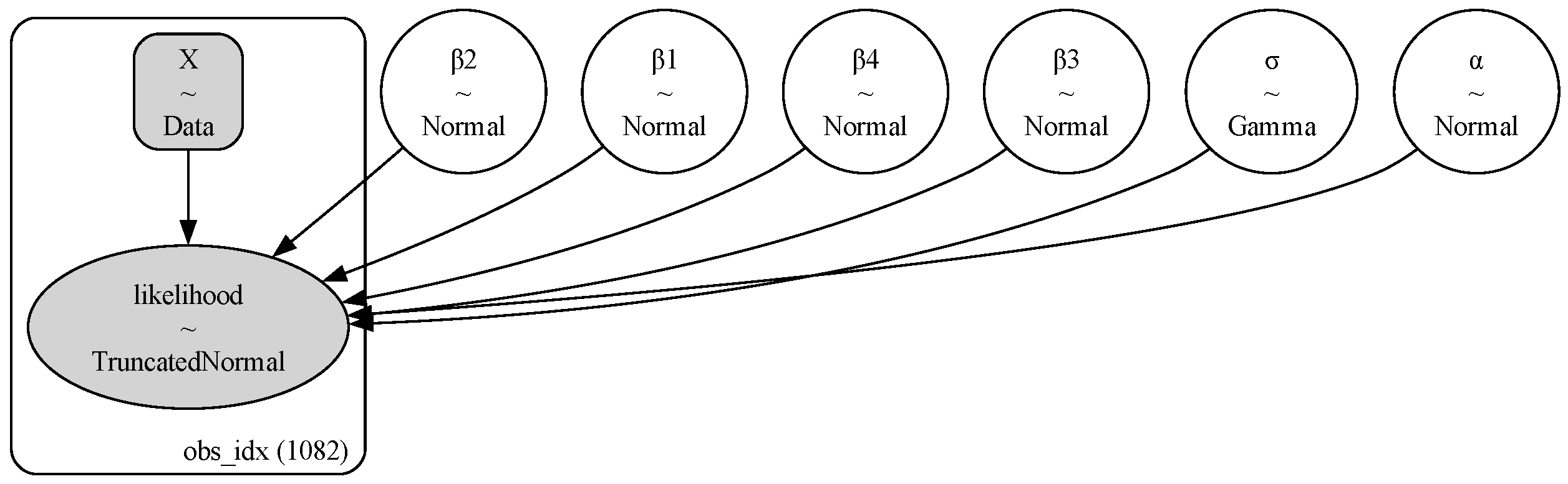
2.2.2. Model Structures and Priors

Model 1 uses a single-level polynomial structure with Gaussian priors on all regression coefficients and a Gamma prior on the shared dispersion parameter $\sigma$. Model 2 introduces a hierarchical structure with group-specific slopes and intercepts based on the dominant MBR numerator band. Unlike the 4th-order polynomial used in Model 1, this model uses a simple linear form and shares information across groups through partial pooling. This added structure is expected to capture spectral variability more effectively and yield improved calibration. Model 5 adds heteroscedasticity by modeling $log\left({\sigma }_i\right)$ as a linear function of log(MBR), with group-specific slopes and intercepts.

All group-level parameters were given Normal priors centered at zero, and hyper-prior standard deviations followed Exponential(1) distributions to allow regularization via partial pooling. Prior predictive checks were performed for all models to ensure reasonable behavior before fitting.

Figure 1 shows the structure of Model 1 as a directed acyclic graph (DAG). DAGs for Models 2 and 5 are provided in the Supplementary Material.

The next section presents results for Models 1, 2, and 5. Extended analyses and diagnostics for all models, including Models 3 and 4, are provided in the Supplementary Materials.

3. Results

3.1. Model Performance Overview

Three models were fit to the data, each extending the previous in structural complexity. Model 1, a Bayesian analogue of OCx-style 4^th order polynomial regression, served as a baseline. Model 2 introduced group-specific structure via hierarchical partial pooling by dominant MBR numerator band. Model 5 extended Model 2 by introducing heteroscedasticity, allowing the dispersion parameter to vary with log(MBR) across groups.

3.2. Model Evaluation: Prior Predictive, Posterior Predictive, and LOO-PIT

Standard evaluation metrics such as $R^2$ or RMSE assess how closely point predictions match observed data. However, these are not appropriate for complete Bayesian model evaluation. These models yield full posterior distributions rather than single-value estimates. Moreover the goal is to approximate the data generation process, not to model data. In this context, predictive accuracy must be judged not only by central tendency but also by how well the model represents uncertainty.

To that end, I evaluate each model using prior and posterior predictive checks and LOO-PIT diagnostics, which respectively assess in-sample fit and out-of-sample calibration. These diagnostics are presented below for Models 1, 2, and 5, beginning with Model 1.

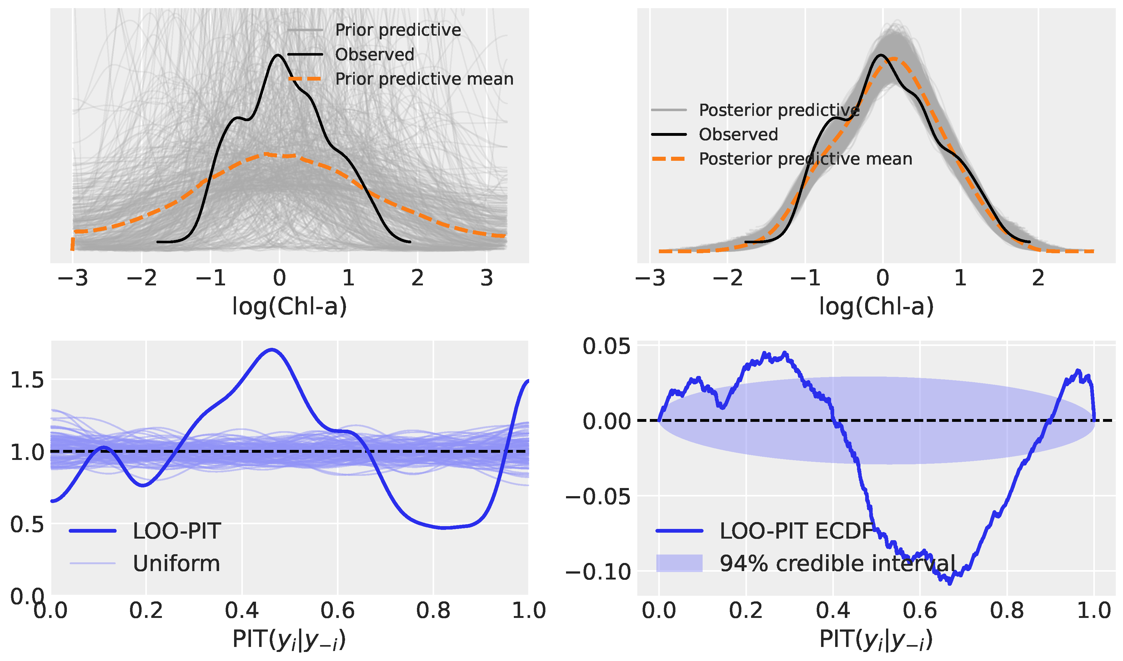
3.2.1. Model 1: Polynomial Regression

The top two panels in Figure 2 display kernel density estimates (KDEs) comparing simulated and observed distributions of log-transformed chlorophyll-a. KDEs provide smoothed estimates of probability density, used to assess how well the model reproduces observed distributions.

The top-left panel shows the prior predictive distribution. Simulated draws from the model under the prior (gray lines) span a wide range of values, as expected given the weakly informative priors. The mean of these simulations (orange dashed line) is diffuse and relatively flat, indicating that the prior allows the model to generate a wide range of plausible outcomes. The observed data KDE (black line) does not influence the prior predictive draws, as the model has not yet been trained on the data; it is included here solely to facilitate comparison with the posterior predictive check in the top-right panel.

The top-right panel compares the posterior predictive distribution to the same observed KDE. The black line represents the empirical distribution of the data, estimated from the NOMAD dataset. It is unimodal, with a dominant peak near log(Chl) = 0 (i.e., 1 mg m⁻³), typical of mesotrophic or moderately productive coastal waters. A secondary shoulder appears near log(Chl) ≈ -0.5, corresponding to lower chlorophyll concentrations (0.3 mg m⁻³ and below) associated with oligotrophic oceanic regions. This structure indicates that the dataset includes a range of ecological regimes, with a skew toward oceanic conditions.

Posterior predictive draws (gray lines) cluster tightly around the observed KDE and differ markedly from the diffuse prior predictive draws, suggesting that the model has learned meaningfully from the data. The posterior predictive mean (orange dashed line) successfully captures the overall support and central tendency of the observed distribution. However, it underestimates the height of the primary mode, and assigns excess probability mass to the shoulders, yielding a flattened peak. This suggests that while the model captures the broad structure of the data, it produces overdispersed predictions, with intervals that are too wide relative to the concentration of observations.

The bottom two panels assess model calibration using leave-one-out probability integral transform (LOO-PIT) diagnostics. Two complementary views are shown: the left panel presents the density of LOO-PIT values via a kernel density estimate (KDE), while the right panel shows the cumulative deviation of those values from the ideal uniform distribution. The KDE is sensitive to local concentration of probability mass—such as over- or underdispersion—while the ECDF-minus-uniform plot emphasizes systematic calibration drift across the distribution. Together, they provide a more complete picture of model uncertainty than either view alone.

The KDE panel (bottom-left) shows the LOO-PIT density (black line) compared against 500 KDEs of values drawn from a uniform distribution (thin blue lines). A horizontal dashed line at $y=1$ denotes the target density for a calibrated model. The observed KDE exhibits a distinct U-shape, with density elevated in the tails and suppressed in the center. This pattern confirms that the model is likely to be overdispersed in out-of-sample prediction: its predictive intervals are too wide, placing too little mass near the typical observations and too much in the extremes.

The bottom-right panel displays the ECDF difference plot, created by subtracting the expected theoretical CDF values (the identity function in [0,1] for standard uniformity) from the observed ECDF values. A horizontal dashed line at $y=0$ references a lack of difference. The shaded band shows a 94% credible interval for this difference under ideal conditions, based on repeated uniform draws. The curve for Model 1 deviates below the reference line in the central quantiles and rises above it in the tails, confirming the pattern seen in the KDE panel. Together, these diagnostics show that while Model 1 captures the central trend of the data, its posterior predictive distributions are too diffuse.

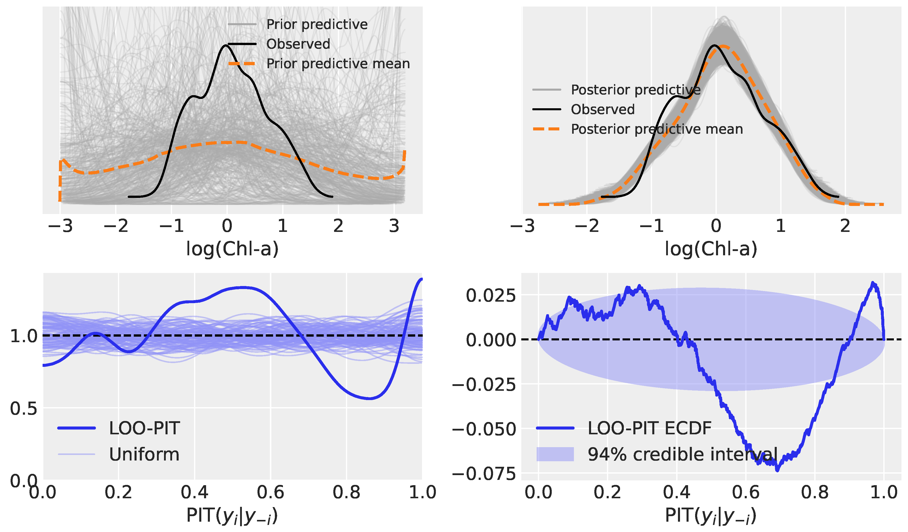
3.2.2. Model 2: Hierarchical Linear Regression

Figure 3 shows the model evaluation panels for Model 2. The prior predictive simulations (top-left) are broader than in Model 1, reflecting the additional flexibility introduced by the hierarchical structure. The prior predictive mean is diffuse, consistent with weakly informative priors to allow for a wide range of generative behaviors.

The posterior predictive check (top-right) shows a notable improvement over Model 1. Posterior draws cluster tightly around the observed KDE, especially near the primary mode. This reflects the effect of partial pooling across MBR groups, which concentrates predictions around dominant patterns in the data. However, the model fails to fully capture the secondary shoulder near $\log \left(\mathrm{Chl}\right)\approx -0.5$, suggesting that some variation remains unaccounted for — possibly due to shrinkage of uncertainty toward the group mean.

As with Model 1, LOO-PIT diagnostics assess out-of-sample calibration. The KDE reveals local deviations from calibration, while the ECDF-minus-uniform plot captures cumulative miscalibration trends. Here, the LOO-PIT diagnostics (bottom row) further support the improved performance. The KDE panel (bottom-left) shows smaller deviations from the uniform reference (dashed line at $y=1$) compared to Model 1. The y-axis range here is narrower—approximately 0.5 to 1.3—indicating that the magnitude of miscalibration is significantly reduced. Similarly, the ECDF-minus-uniform plot (bottom-right) shows deviations that remain well within the 94% credible interval, with a y-axis span of just ±0.025. These compressed ranges reflect a more calibrated model. Mild signs of overdispersion persist—visible as a small negative dip in the central quantiles—but overall, Model 2 represents a substantial improvement in both fit and uncertainty calibration relative to the baseline.

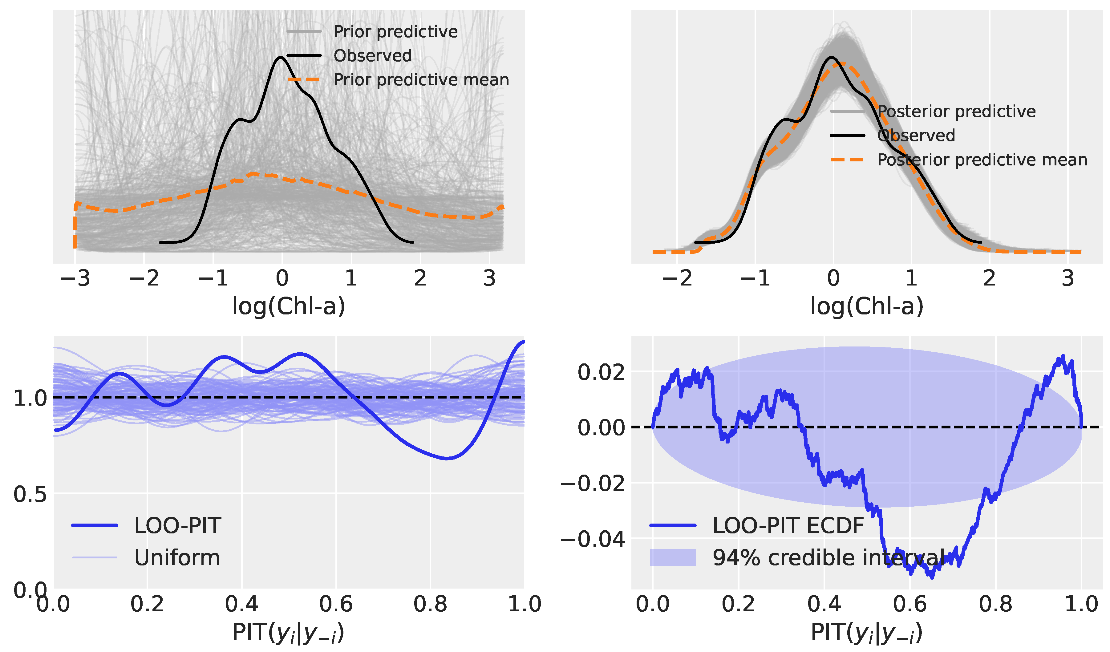
3.2.3. Model 5: Heteroscedastic Hierarchical Linear Regression

Model 5 extends the hierarchical structure of Model 2 by allowing the likelihood variance $\sigma$ to vary linearly with log(MBR), using group-specific intercepts and slopes. This accommodates heteroscedasticity across spectral groups and better reflects the variance structure of the data. By explicitly modeling the dispersion, the model is expected to improve both fit and calibration, particularly in the tails of the predictive distribution.

Figure 4 presents the four-panel evaluation for Model 5. The prior predictive simulations (top-left) are the most diffuse of any model—expected, given the added flexibility in both the mean and variance components. The prior predictive mean (orange dashed line) is nearly flat. As before, the observed KDE (black line) is included only for visual comparison. The posterior predictive check (top-right) shows excellent agreement between the posterior draws and the observed KDE. The model captures both the main mode near $\log \left(\mathrm{Chl}\right)=0$ and the secondary shoulder near -0.5—something neither Model 1 nor 2 accomplished. The predictive mean aligns closely with the observed distribution, and the vertical spread among draws reflects uncertainty in both the mean and variance terms.

For Model 5 the bottom-left LOO-PIT panel shows a nearly flat density centered around the ideal reference line at $y=1$ , with minor undulations well within the light blue band representing draws from the uniform distribution. The vertical range is now the tightest of all three models and indicates minimal deviation from ideal calibration. The ECDF deviance (bottom-right panel) shows similarly tight behavior. The LOO-PIT curve remains entirely within the 94% credible interval and deviates by no more than ±0.02 from the reference line at $y=0$. Together, these diagnostics suggest that Model 5 is the best calibrated and most accurate of all models developed in this study.

3.3. Predictive Coverage

Posterior predictive intervals represent a core strength of Bayesian modeling: the ability to express uncertainty in probabilistic terms. A 94% highest density interval (HDI) reflects a direct statement about the distribution of predicted outcomes:

“Given a specific input, there is a 94% probability that the outcome lies within this interval, conditioned on the model and the data.”

This stands in contrast to frequentist confidence intervals or classical machine learning point predictions, which provide no such probabilistic guarantee. Instead of merely reporting central tendencies or summary error metrics, Bayesian predictive intervals communicate how confident the model is about each individual prediction.

Figure 5, Figure 6 and Figure 7 visualize this by overlaying 94% HDI on scatter plots of observed log-transformed chlorophyll-a concentrations. Shaded ribbons represent the predicted HDI at each value of log(MBR), stratified by MBR numerator group. If a model represents the data-generating process well, the HDI should envelop the bulk of the observations, adjusting their width to reflect changes in uncertainty across the covariate space.

This kind of distribution-aware predictive structure is essential in scientific contexts like ocean color remote sensing, where quantifying uncertainty is as important as making accurate predictions.

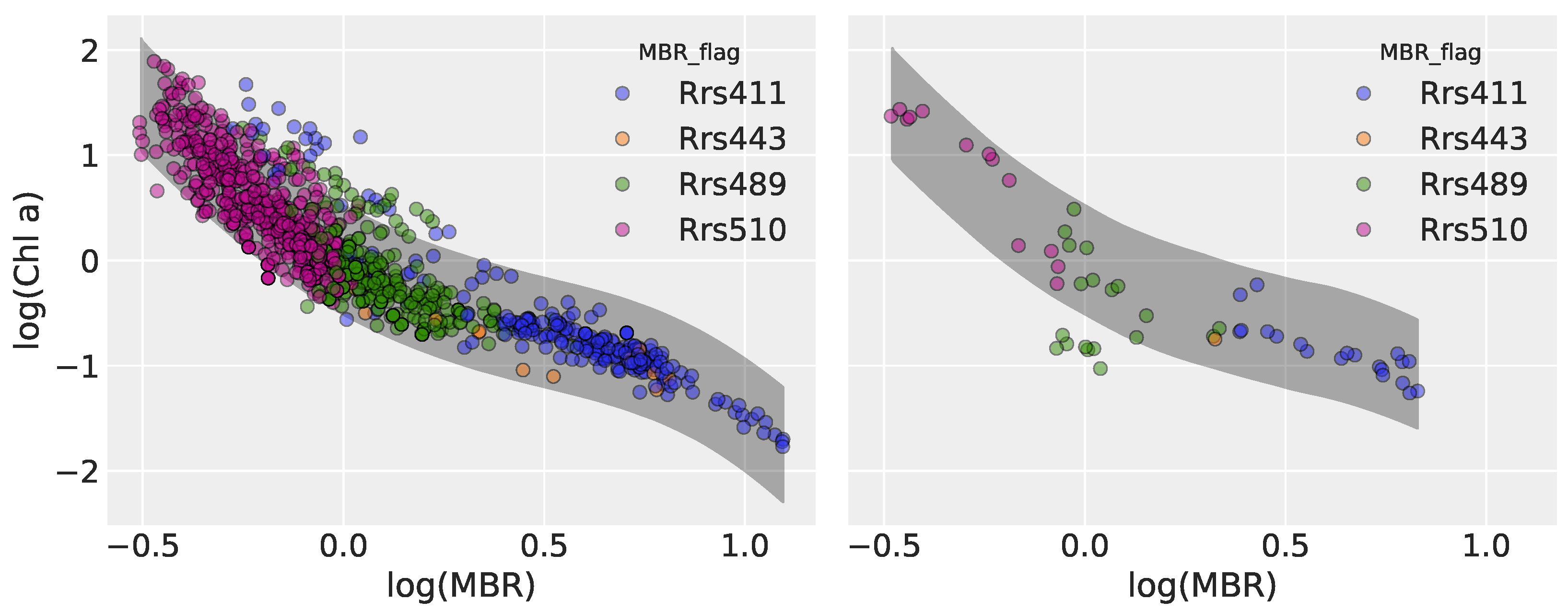
3.3.1. Model 1

Figure 5 shows the 94% posterior predictive intervals from Model 1 overlaid on the observed log-transformed chlorophyll-a values, stratified by dominant MBR numerator band. Because this model uses a constant dispersion term ($\sigma$), the predictive intervals maintain a uniform width across log(MBR), regardless of local data density or group-specific trends.

In the in-sample (NOMAD) panel, the HDI bands roughly follow the central trend of the data but ignore group-specific patterns. Some groups are captured in the middle of the log(MBR) range, but coverage deteriorates in the tails, where intervals are either too wide or too narrow depending on the group.

In the out-of-sample (SeaBASS) panel, the model often fails to cover held-out observations, particularly at low and high values of log(MBR). A cluster of six Rrs(489) group observations falls below the 94% HDI band.

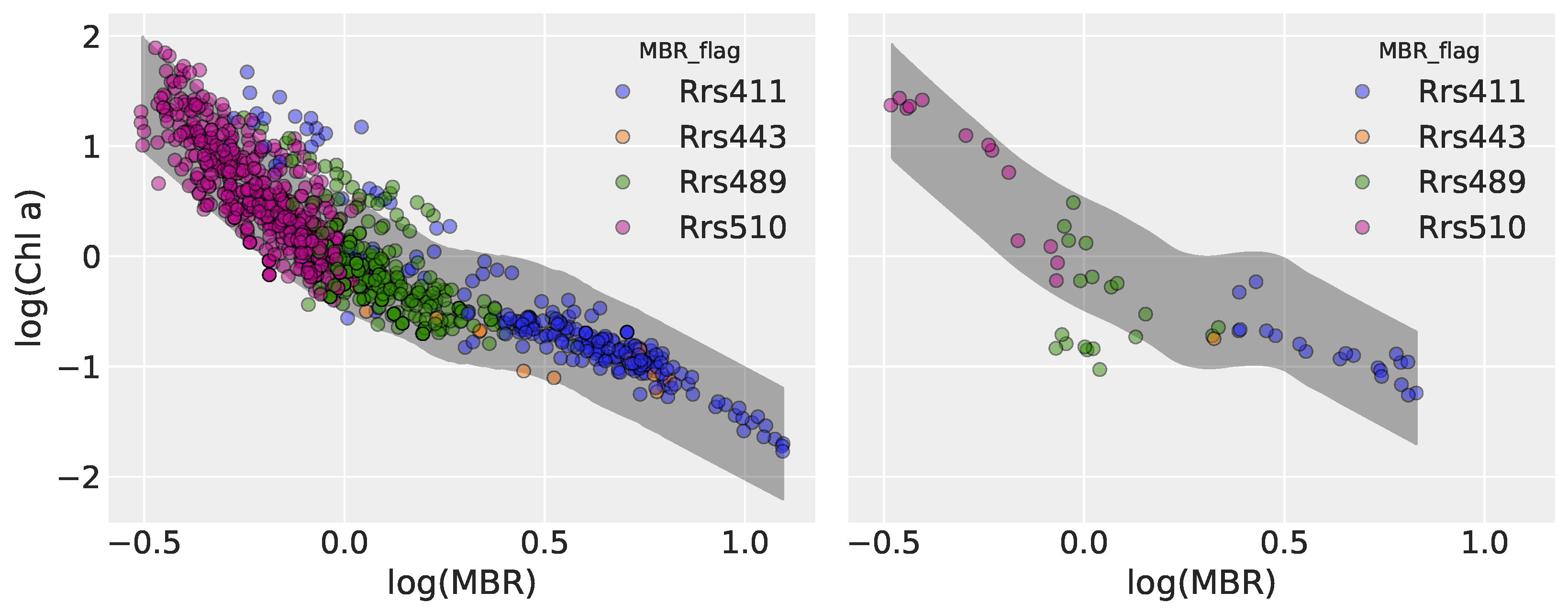
3.3.2. Model 2

Figure 6 shows predictive coverage plots for Model 2, which introduces group-specific linear fits via a hierarchical structure. This partial pooling allows the model to share information across MBR numerator groups while still learning distinct intercepts and slopes for each.

In the in-sample coverage, the HDI bands now reflect different mean relationships across groups. This better matches the stratified nature of the data and corrects for the uniformity of the polynomial fit in Model 1. However, the interval width remains constant within each group, as the model still uses a shared, homoskedastic dispersion term. As a result, although the predicted means improve, the HDI bands still fail to capture group-specific differences in variance.

In the SeaBASS panel, the model shows improved group-wise trend fitting, but the same Rrs(489) cluster remains outside the HDI range, as in Model 1.

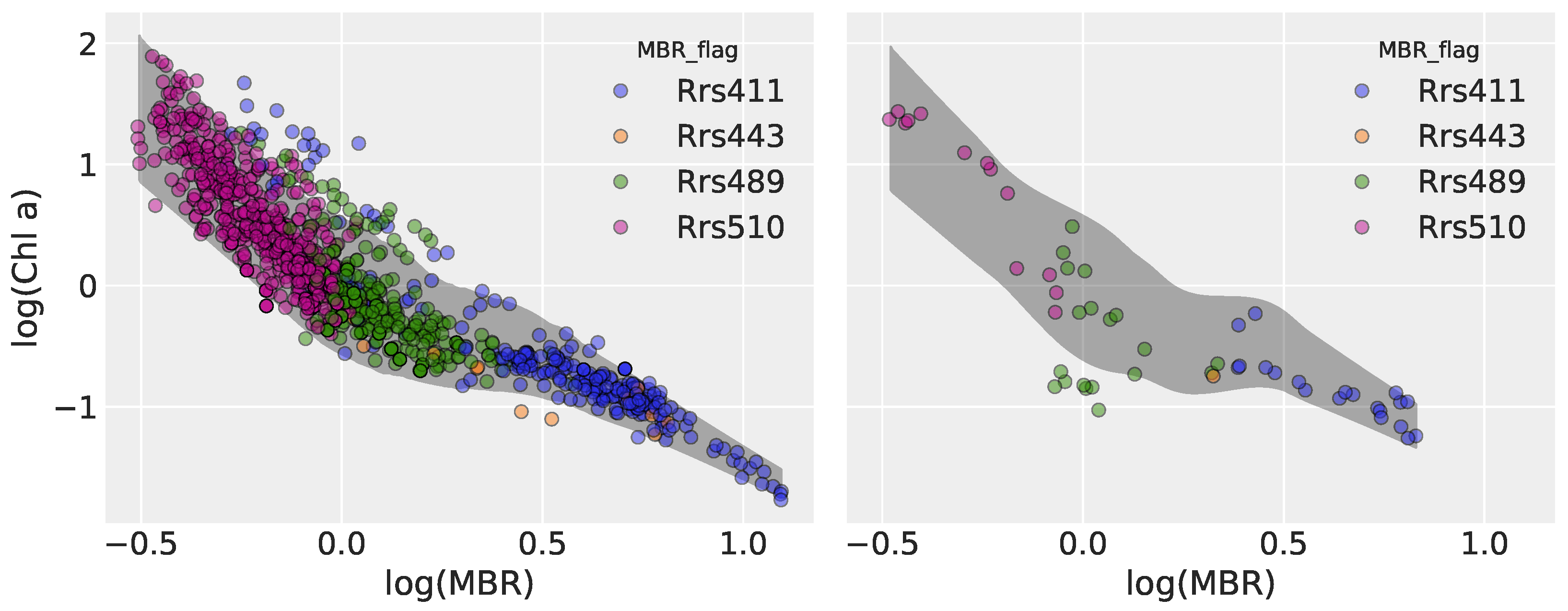
3.3.3. Model 5

Figure 7 shows the predictive coverage for Model 5, which retains the group-specific linear structure of Model 2 and introduces heteroscedasticity by modeling log($\sigma$) as a linear function of log(MBR), with group-specific intercepts and slopes. This structure allows the posterior predictive intervals to vary in both shape and width across the predictor space and between groups.

In the NOMAD dataset (left panel), the HDI bands closely follow the observed spread for most groups and values of log(MBR), suggesting that the model has captured both the mean trends and variance structures. However, two points belonging to the Rrs(443) group fall below the lower edge of the 94% HDI, indicating that the model slightly overestimates chlorophyll-a for these observations. While localized, these deviations highlight that even overall better calibrated models may still fail to capture rare configurations within a group.

In the SeaBASS dataset (right panel), Model 5 shows overall strong alignment between predictive intervals and held-out observations. The HDI bands vary in shape and width across log(MBR) and MBR groups, indicating that the model has captured key aspects of input-dependent variance. Most groups show good coverage across the covariate range.

However, as with Models 1 and 2, a cluster of six observations in the Rrs(489) group consistently falls below the 94% HDI band. The shape of the HDI does not adjust to encompass these points, suggesting a consistent mismatch between predicted and observed values for this subset of the test data.

Overall, each increase in model complexity yielded clear improvements in predictive performance. Model 2 corrected the uniform mean structure of Model 1 by incorporating group-specific fits, though its constant-width intervals failed to capture variance differences. Model 5 extended this framework with heteroscedasticity, allowing both mean and variance to vary across groups, and achieved the best overall predictive coverage. Nonetheless, localized mismatches—such as the persistent Rrs(489) cluster—remained, underscoring the limits of even the most flexible model considered here.

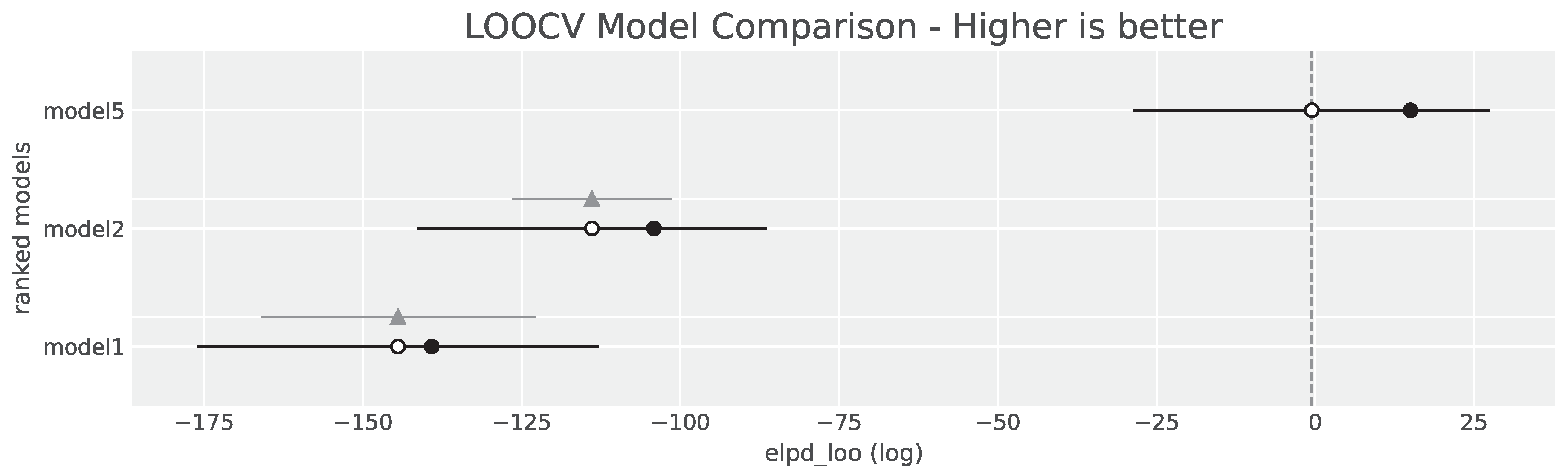
3.4. Model Comparison

PSIS-LOO results are summarized in Table 2 and visualized in Figure 8. Among the three models evaluated, Model 5 achieved the highest expected log predictive density (ELPD_LOO), indicating the best expected out-of-sample predictive performance. Model 2 ranked second, with an ELPD difference of 113.39 relative to Model 5, while Model 1 ranked third with an ELPD difference of 143.94. Model complexity is represented by the effective number of parameters ($p_{\mathrm{loo}}$), which quantifies the model’s flexibility as estimated from the posterior distribution. This measure is derived from the variance in the pointwise log-likelihood and reflects the degree to which the model adapts to the observed data. Across the three models, $p_{\mathrm{LOO}}$ increased from 5.32 in Model 1 to 15.55 in Model 5. Model 5 also had the highest model weight (0.96), indicating strong preference under the PSIS-LOO criterion.

Overall, increasing model complexity was associated with improvements in calibration and predictive performance on aggregate diagnostics, while predictive coverage revealed a small number of localized deviations that persist across models; a cluster belonging to the Rrs(489) group of the out-of-sample data.

4. Discussion

4.1. Summary of Findings

This study demonstrates the application of a complete Bayesian workflow to a foundational ocean color chlorophyll-a retrieval problem. Building from a Bayesian analogue of the OCx-style polynomial regression, I progressively increased model complexity by introducing hierarchical structure across maximum band ratio (MBR) groups (Model 2) and subsequently allowing heteroscedasticity via group-specific variance models (Model 5). Across all evaluation metrics—prior and posterior predictive checks, LOO-PIT calibration diagnostics, predictive coverage, and PSIS-LOO model comparison—each successive model displayed measurable improvements in calibration and predictive accuracy. Model 5, the most complex in the series, achieved the highest expected log predictive density and the most consistent calibration across both training and held-out data.

While overall calibration improved with model complexity, localized deviations remained. In particular, a cluster of six $\mathrm{Rrs}\left(489\right)$ points from the SeaBASS dataset fell below the 94% highest density interval (HDI) across all models, and two $\mathrm{Rrs}\left(443\right)$ points in NOMAD moved outside the HDI in Model 5 despite being covered in simpler models. These exceptions highlight the need for targeted model extensions to fully capture structured predictive mismatches.

4.2. Comparison with Classical and Machine Learning Approaches

Unlike traditional chlorophyll-a retrieval algorithms or classical machine learning regressors, the Bayesian models presented here yield full posterior distributions over parameters and predictions. This framework enables direct probabilistic statements about prediction intervals—e.g., “given the data and model, there is a 94% probability that the true value lies within this interval”—that are unavailable in frequentist point-estimation frameworks.

Evaluation metrics such as $R^2$, RMSE, or MAE, commonly used in both classical regression and ocean color algorithm validation [15], measure only point-prediction accuracy. They neither leverage the full posterior distribution nor account for model complexity. By contrast, Pareto-smoothed importance sampling leave-one-out cross-validation (PSIS-LOO) evaluates predictive performance using the entire posterior and adjusts for model complexity via the effective number of parameters ($p_{\mathrm{LOO}}$). This complexity penalty reduces the risk of overfitting and allows fairer comparison between models of differing flexibility, similar in spirit to but more robust than information criteria such as AIC.

Classical machine learning regression models, including ensembles such as random forests or boosting methods, can flexibly fit nonlinear relationships but typically discard uncertainty unless specifically extended (e.g., through ensembles, dropout, or Bayesian variants). In contrast, Bayesian models natively quantify both parameter and predictive uncertainty, providing calibrated probability statements rather than only central predictions or heuristic confidence estimates.

4.3. Sources of Predictive Mismatch

Inspection of predictive coverage plots revealed several persistent patterns of mismatch. Most notably, a group of six $\mathrm{Rrs}\left(489\right)$ points in the SeaBASS dataset consistently fell below the lower bound of the 94% HDI for all models. This indicates a systematic bias for this subset that is not explained by the current grouping structure. In the NOMAD dataset, two $\mathrm{Rrs}\left(443\right)$ points fell below the HDI only in Model 5, suggesting that increased complexity can occasionally overfit certain relationships, leading to localized loss of coverage. Such patterns imply that the current grouping by dominant MBR numerator, while capturing important structure, omits additional sources of variance, likely tied to sensor-specific or environmental factors.

4.4. Future Directions

The patterns of predictive mismatch identified here point toward several avenues for extending the present modeling framework.

First, the hierarchical structure could be expanded to include additional grouping variables—notably satellite sensor type—while also allowing heteroscedasticity to vary across these new dimensions. Such an approach would help capture systematic offsets in the reflectance–chlorophyll relationship arising from differences in spectral response functions, radiometric calibration, or atmospheric correction methodology. Crossed or nested random effects could enable simultaneous partial pooling across MBR groups and sensor categories, while variance terms could flexibly adapt to subsets of the data that exhibit systematically different levels of uncertainty.

Second, incorporating the full interband covariance structure offers a promising path to improved predictions. By treating the set of relevant spectral bands as a multivariate predictor, the model could exploit correlations among reflectances to resolve cases where univariate MBR-based predictors are insufficient. This could be implemented either through a multivariate regression framework or via direct modeling of the joint distribution of spectral inputs.

Together, these extensions would enhance the model’s ability to represent both the central tendency and the uncertainty of chlorophyll-a predictions, reducing systematic mismatches and further aligning predictive coverage with the underlying data-generating process.

4.5. Concluding Remarks

By recasting a foundational chlorophyll-a retrieval problem within a fully Bayesian framework, this study illustrates the value of a complete workflow that integrates prior predictive checks, posterior predictive diagnostics, calibration assessment via LOO-PIT, and complexity-adjusted model comparison using PSIS-LOO. The results show that accounting for both group-level structure and heteroscedasticity can substantially improve predictive calibration and the representation of uncertainty. At the same time, persistent localized mismatches highlight opportunities for targeted model extensions, particularly through the inclusion of additional grouping variables and the exploitation of spectral covariance. Together, these refinements point toward more reliable and interpretable chlorophyll-a products from satellite ocean color data, supporting the broader goal of uncertainty-aware remote sensing for marine ecosystem monitoring. An additional advantage of the Bayesian approach is that existing posteriors can be updated as new data become available, ensuring that models remain current as observing systems and in-situ matchups continue to grow.

References

- O’Reilly, J.E.; Maritorena, S.; Mitchell, B.G.; Siegel, D.A.; Carder, K.L.; Garver, S.A.; Kahru, M.; McClain, C. Ocean color chlorophyll algorithms for SeaWiFS. Journal of Geophysical Research: Oceans 1998, 103, 24937–24953. [CrossRef]
- O’Reilly, J.E.; Maritorena, S.; Siegel, D.A.; O’Brien, M.C.; Toole, D.; Mitchell, B.G.; Kahru, M.; Chavez, F.P.; Strutton, P.; Cota, G.F.; et al. Ocean color chlorophyll a algorithms for SeaWiFS, OC2, and OC4: Version 4. SeaWiFS postlaunch calibration and validation analyses, Part 2000, 3, 9–23.
- Hu, C.; Lee, Z.; Franz, B. Chlorophyll aalgorithms for oligotrophic oceans: A novel approach based on three-band reflectance difference. Journal of Geophysical Research: Oceans 2012, 117. [CrossRef]
- O’Reilly, J.E.; Werdell, P.J. Chlorophyll algorithms for ocean color sensors - OC4, OC5 & OC6. Remote Sensing of Environment 2019, 229, 32–47. [CrossRef]
- Jaynes, E.; Bretthorst, G. Probability Theory: The Logic of Science; Cambridge University Press, 2003.
- Scheemaekere, X.D.; Szafarz, A. The Inference Fallacy From Bernoulli to Kolmogorov, 2011. CEB Working Paper N° 11/006, February 2011.
- Clayton, A. Bernoulli’s Fallacy: Statistical Illogic and the Crisis of Modern Science; Columbia University Press, 2022.
- Baker, M. 1,500 scientists lift the lid on reproducibility. Nature 2016, 533, 452–454. [CrossRef]
- Cobey, K.D.; Ebrahimzadeh, S.; Page, M.J.; Thibault, R.T.; Nguyen, P.Y.; Abu-Dalfa, F.; Moher, D. Biomedical researchers’ perspectives on the reproducibility of research. PLoS biology 2024, 22, e3002870.
- Gal, Y. Uncertainty in Deep Learning. PhD thesis, University of Cambridge, 2016.
- Ghahramani, Z. Probabilistic machine learning and artificial intelligence. Nature 2015, 521, 452–459.
- Werther, M.; Burggraaff, O. Dive Into the Unknown: Embracing Uncertainty to Advance Aquatic Remote Sensing. Journal of Remote Sensing 2023, 3, 0070. [CrossRef]
- Bishop, C.M. Pattern Recognition and Machine Learning; Springer, 2006.
- Gruber, C.; Schenk, P.O.; Schierholz, M.; Kreuter, F.; Kauermann, G. Sources of Uncertainty in Supervised Machine Learning – A Statisticians’ View, 2025, [arXiv:stat.ML/2305.16703].
- Seegers, B.N.; Stumpf, R.P.; Schaeffer, B.A.; Loftin, K.A.; Werdell, P.J. Performance metrics for the assessment of satellite data products: an ocean color case study. Opt. Express 2018, 26, 7404–7422. [CrossRef]
- Frouin, R.; Pelletier, B. Bayesian methodology for inverting satellite ocean-color data. Remote Sensing of Environment 2015, pp. 332–360. [CrossRef]
- Shi, Y.; Zhou, X.; Yang, X.; Shi, L.; Ma, S. Merging Satellite Ocean Color Data With Bayesian Maximum Entropy Method. IEEE Journal of Selected Topics in Applied Earth Observations and Remote Sensing 2015, 8, 3294–3304. [CrossRef]
- Craig, S.E.; Karaköylü, E.M. Bayesian Models for Deriving Biogeochemical Information from Satellite Ocean Color. EarthArXiv 2019. [CrossRef]
- Werther, M.; Odermatt, D.; Simis, S.G.H.; Gurlin, D.; Lehmann, M.K.; Kutser, T.; Gupana, R.; Varley, A.; Hunter, P.D.; Tyler, A.N.; et al. A Bayesian approach for remote sensing of chlorophyll-a and associated retrieval uncertainty in oligotrophic and mesotrophic lakes. Remote Sensing of Environment 2022, 283, 113295. [CrossRef]
- Werther, M.; Burggraaff, O.; Gurlin, D.; Saranathan, A.M.; Balasubramanian, S.V.; Giardino, C.; Braga, F.; Bresciani, M.; Pellegrino, A.; Pinardi, M.; et al. On the generalization ability of probabilistic neural networks for hyperspectral remote sensing of absorption properties across optically complex waters. Remote Sensing of Environment 2025, 328, 114820. [CrossRef]
- Erickson, Z.K.; McKinna, L.I.W.; Werdell, P.J.; Cetinić, I. Bayesian approach to a generalized inherent optical property model. Optics Express 2023, 31, 22790 – 22801. [CrossRef]
- Gelman, A.; Vehtari, A.; Simpson, D.; Margossian, C.C.; Carpenter, B.; Yao, Y.; Kennedy, L.; Gabry, J.; Bürkner, P.C.; Modrák, M. Bayesian Workflow, 2020, [arXiv:stat.ME/2011.01808].
- Wolkovich, E.; Davies, T.J.; Pearse, W.D.; Betancourt, M. A four-step Bayesian workflow for improving ecological science, 2024, [arXiv:q-bio.QM/2408.02603].
- JCGM. Evaluation of Measurement Data – Guide to the Expression of Uncertainty in Measurement. Technical Report JCGM 100:2008, Joint Committee for Guides in Metrology (JCGM), Sèvres, France, 2008. GUM 1995 with minor corrections.
- Tilstone, G.; Mélin, F.; Jackson, T.; Valente, A.; Bailey, S.; Moore, T.; Kahru, M.; Boss, E.; Mitchell, B.G.; Wang, M.; et al. Uncertainties in Ocean Colour Remote Sensing. Technical Report Report 18, International Ocean Colour Coordinating Group (IOCCG), Dartmouth, Canada, 2020. IOCCG Report Series, 124 pp.
- Werdell, P.; Bailey, S. An improved bio-optical data set for ocean color algorithm development and satellite data product validation. Remote Sensing of Environment 2005, 98, 122–140.
- Abril-Pla, O.; Andreani, V.; Carroll, C.; Dong, L.; Fonnesbeck, C.J.; Kochurov, M.; Kumar, R.; Lao, J.; Luhmann, C.C.; Martin, O.A.; et al. PyMC: a modern, and comprehensive probabilistic programming framework in Python. PeerJ Computer Science 2023, 9, e1516. [CrossRef]
- Homan, M.D.; Gelman, A. The No-U-turn sampler: adaptively setting path lengths in Hamiltonian Monte Carlo. J. Mach. Learn. Res. 2014, 15, 1593–1623.
- McElreath, R. Statistical Rethinking: A Bayesian Course with Examples in R and Stan, 2 ed.; CRC Press, 2020.
- Säilynoja, T.; Bürkner, P.C.; Vehtari, A. Graphical test for discrete uniformity and its applications in goodness-of-fit evaluation and multiple sample comparison. Statistics and Computing 2022, 32. [CrossRef]
- Nguyen, A.B.; Bonici, M.; McGee, G.; Percival, W.J. LOO-PIT: A sensitive posterior test. Journal of Cosmology and Astroparticle Physics 2025, 2025, 008. [CrossRef]
- Vehtari, A.; Simpson, D.; Gelman, A.; Yao, Y.; Gabry, J. Pareto Smoothed Importance Sampling, 2024, [arXiv:stat.CO/1507.02646].
- Vehtari, A.; Gelman, A.; Gabry, J. Practical Bayesian model evaluation using leave-one-out cross-validation and WAIC. Statistics and Computing 2016, 27, 1413–1432. [CrossRef]