Submitted:
27 August 2025
Posted:
28 August 2025
You are already at the latest version
Abstract
Frequent channel migrations of the Yellow River coupled with increasing human disturbances have been driven significant land cover changes in the Yellow River Delta (YRD) over time. Accurate estimation of aboveground biomass (AGB) and clarification of the impact of land cover changes on AGB are crucial for monitoring vegetation dynamics and supporting ecological management. However, field-based biomass samples are often time-consuming and labor-intensive, and the quantity and quality of such samples greatly affects the accuracy of AGB estimation. This study developed a robust AGB estimation framework for the YRD by synthesizing 4,717 field-measured samples from published scientific literature and integrating two critical ecological indicators: leaf aera index (LAI) and length of growing season (LGS). A random forest (RF) model was employed to estimate AGB for the YRD from 2001 to 2022, achieving high accuracy (R² = 0.74). The results revealed a continuous spatial expansion of AGB over the past two decades, with higher biomass consistently observed in western cropland and along the Yellow River, whereas lower biomass levels were concentrated in areas south of the Yellow River. AGB followed a fluctuating upward trend, reaching a minimum of 204.07 g/m² in 2007, peaking at 230.79 g/m² in 2016, and stabilizing thereafter. Spatially, western areas showed positive trends, with an average annual increase of approximately 10 g/m², whereas central and coastal zones exhibited localized declines of around 5 g/m². Among the changes in land cover, cropland and wetlands changes were the main contributors to AGB increases, accounting for 54.2% and 52.67%, respectively. In contrast, grassland change exhibited limited or even suppressive effects, contributing −6.87% to the AGB change. Wetlands showed the greatest volatility in the interaction between area change and biomass density change, which is the most uncertain factor in the dynamic change of AGB.
Keywords:
aboveground biomass
; herbaceous
; Yellow River Delta
; spatiotemporal dynamics
; remote sensing mapping
1. Introduction
Herbaceous vegetation, dominant in grassland, wetlands, and cropland system, contributes significantly to biodiversity, soil stabilization, and nutrient cycling [1]. These plants are vital in carbon sequestration processes, acting as short-term carbon sinks and influencing local microclimates [2]. Understanding the distribution, productivity, and ecological functions of herbaceous plants is therefore critical for sustainable land management, biodiversity conservation, and climate change mitigation. Among the various ecological attributes of herbaceous vegetation, aboveground biomass (AGB) is a key biophysical indicator representing vegetation productivity, ecosystem functioning, and carbon sequestration potential [3]. AGB refers to the total mass of living plant material above the soil surface and is essential for assessing vegetation health, land degradation, and carbon dynamics under changing climatic conditions [4]. However, traditional methods for obtaining AGB are time-consuming and labor-intensive, highlighting the need for more efficient and scalable approaches to AGB estimation.
Satellite remote sensing has emerged as the preferred approach for large-scale herbaceous AGB monitoring, offering repeated, spatially continuous, and cost-effective observations [5]. A commonly used approach for AGB estimation involves establishing empirical models that correlate field-measured AGB with spectral bands and vegetation indices (VIs) derived from remote sensing imagery [6]. While this method is straightforward, intuitive, and computationally simple, it often fails to fully exploit the rich spectral information contained in multispectral or hyperspectral data [7]. With advancements in remote sensing technologies, a variety of vegetation-related ecological indicators, such as leaf area index (LAI) and length of growing season (LGS), have become available. LAI is one of the important parameters for monitoring crop growth status, a concept closely related to photosynthesis, respiration, transpiration, and a series of environmental interaction processes such as carbon cycle and precipitation interception. Moreover, LAI is an effective index for diagnosing crop growth, estimating biomass, and predicting yield [8,9,10]. LGS represents the period from the onset of vegetation growth to maturity, which is a critical phase for carbon fixation and is closely associated with biomass accumulation. Moreover, LGS reflects local climatic conditions. Seasonal variations in climate factors such as precipitation can alter vegetation phenology, which in turn affects terrestrial carbon cycle [11,12]. These indicators effectively capture the growth status of vegetation and hold great potential for improving the accuracy of biomass estimation models [13,14,15].
Compared with empirical models for AGB estimation, machine learning (ML) algorithms have demonstrated superior performance due to their strong capabilities in handling high-dimensional data, capturing complex nonlinear relationships, and automating feature learning processes [13]. Among various ML algorithms, the random forest (RF) algorithm has become one of the most widely used and consistently effective methods in remote sensing-based AGB estimation[16,17,18]. RF is an ensemble learning method that constructs multiple decision trees and aggregates their predictions, which greatly enhances model stability and reduces the risk of overfitting [19]. In addition, it is capable of handling large volumes of heterogeneous data and capturing complex nonlinear interactions among variables[20]. Existing studies demonstrate that RF often outperforms other algorithms in terms of model accuracy and robustness, making it a preferred choice for vegetation biomass mapping [21].
However, the accuracy of AGB estimation based on ML algorithms is highly influenced by the availability of sufficient and reliable field-measured biomass samples. In addition, Large-scale field sampling is often constrained by limited resources, high costs, and logistical challenges, especially in remote or ecologically sensitive areas [22].Fortunately, numerous studies have focused on biomass monitoring, and many of them contain ample field sampling data reported in peer-reviewed publications [23,24,25]. These openly accessible studies provide a valuable source of field data, including detailed measurements, sampling dates, and geographic locations, making it feasible to compile a robust ground-truth dataset. Therefore, we propose extracting biomass sample data through literature review to address the insufficient sampling issue in AGB estimation and spatiotemporal mapping.
The Yellow River Delta (YRD), located in eastern China, serves as an ideal case study for herbaceous AGB estimation. As one of the youngest and most dynamic coastal wetland ecosystems in the world, the YRD features vast expanses of artificial croplands, natural grasslands, and restored wetlands [26]. The region plays a crucial ecological role in biodiversity conservation, shoreline stabilization, and carbon storage. However, over the past few decades, the YRD has experienced increasing ecological pressures from climate change, hydrological disruptions, and human activities, resulting in vegetation degradation and frequent land cover conversions [27]. In this context, the accurate estimation of herbaceous AGB is not only essential for monitoring vegetation productivity and restoration outcomes, but also critical for assessing regional carbon stocks, evaluating grassland quality, and guiding sustainable land-use practices in deltaic environments.
Accordingly, this study aims to develop an efficient, scalable, and accurate framework for estimating herbaceous AGB in the YRD. The primary objectives are to (1) construct a robust AGB estimation model by incorporating field data from literature and integrating two critical ecological indicators: leaf area index (LAI) and length of growing season (LGS); (2) analyze the spatiotemporal dynamics of AGB over the past two decades; and (3) investigate the effects of land cover changes on biomass variability. The findings are expected to support long-term ecological monitoring, improve our understanding of vegetation dynamics, and provide scientific references for wetland conservation and regional ecosystem management.
2. Materials
2.1. Study Area
The Yellow River Delta (YRD), located in northeastern Shandong Province, China (118°07′–119°10′E, 36°55′–38°12′N), covers approximately 5,934 km². With a sub-humid continental monsoon climate, the region experiences annual precipitation of 530–630 mm (mainly from May to September) and high evapotranspiration (700–2400 mm), resulting in saline soils that constrain tree growth [27]. The terrain is low and gently undulating (1–2 m above sea level), shaped by frequent channel migrations of the Yellow River and characterized by micro-topographic features such as levees, depressions, and slopes. Due to the harsh soil and hydrological conditions, the area is dominated by salt-tolerant herbaceous vegetation [28].
2.2. Field Data
This study extracted field-measured aboveground biomass (AGB) data from published scientific literature. A literature search was conducted on the Web of Science (WOS) using the topic keywords “biomass” and “grassland or shrub or cropland”. To improve efficiency and ensure data relevance, the results were sorted by relevance. A total of 7,970 publications related to biomass were initially identified, covering the period from 2010 to 2022. Each article was manually reviewed, and biomass information, along with the corresponding sampling time and geographic coordinates, was extracted from figures and tables. The AGB measurements recorded in the selected studies followed broadly consistent protocols: selecting vegetation plots of appropriate size, harvesting the aboveground parts of plants, oven-drying the samples to obtain dry biomass weight, and recording accurate geographic coordinates and sampling dates [29]. Only biomass data that explicitly described scientifically sound field sampling procedures were considered. To ensure spatiotemporal accuracy, sampling dates were required to be specified at least to the month, and spatial coordinates were required to have a precision of at least 30″. Since the collected biomass data were reported in various units, all measurements were standardized to g/m². For records providing only the month and a coordinate range, the midpoint of the given range was used. Although the process of extracting data from literature represents a substantial effort, it offers greater efficiency and flexibility compared with field sampling, allowing the compilation of large datasets in a relatively short time.
In the data preprocessing stage, obvious erroneous records, such as those located outside terrestrial areas, were manually removed. Since most samples were collected within specific study sties or experimental plots, additional filtering was necessary to exclude points lacking broader representativeness. To this end, Local Moran’s I was applied to assess spatial autocorrelation [30].by comparing the attribute value of each point with the mean of its neighboring points, spatial outliers were identified and removed. In addition, to remove noise and improve data quality, the interquartile range (IQR) method was employed to detect and eliminate outliers. Duplicate records were also identified and removed to ensure that the dataset consisted of independent, high-quality observations suitable for regression analysis. After excluding inconsistent or unreliable entries, as well as clearly erroneous entries, a total of 4,717 valid sampling points were retained. As the original biomass distribution exhibited strong left skewness, a logarithmic transformation was applied to normalize the data (Figure 1).
2.3. Remote Sensing Data
2.3.1. Reflectance and Vegetation Index
The reflectance data were derived from the Landsat satellite series and accessed via the Google Earth Engine (GEE) platform. In this study, we utilized atmospherically corrected surface reflectance data from Landsat 5 Thematic Mapper (TM), Landsat 7 Enhanced Thematic Mapper Plus (ETM+), and Landsat 8 Operational Land Imager (OLI) spanning the period 2001–2022. The Landsat series provide a 30-meter spatial resolution with a 16-day revisit cycle, offering an optimal balance between spatial detail and temporal frequency for monitoring vegetation dynamics across large areas. GEE provides Landsat surface reflectance products (Level-2), generated after radiometric calibration and atmospheric correction [31]. As for Atmospheric correction, Landsat 5 TM and 7 ETM+ use LEDAPS based on the 6S radiative transfer model [32,33], and Landsat 8 OLI applies LaSRC, which relies on MODTRAN with enhanced aerosol inversion and BRDF adjustments [34,35]. According to the different advantages of each VI in reflecting vegetation growth, various VIs such as Normalized Difference Vegetation Index (NDVI), Ratio Vegetation Index (RVI), Enhanced Vegetation Index (EVI), Two-band Enhanced Vegetation Index (EVI2), Difference Vegetation Index (DVI), Soil-Adjusted Vegetation Index (SAVI), Optimized Soil-Adjusted Vegetation Index (OSAVI), Modified Soil-Adjusted Vegetation Index (MSAVI), and Normalized Difference Phenology Index (NDPI) were calculated from Landsat surface reflectance products through GEE platform [36,37] (Table 1).
2.3.2. Land Cover Data
Frequent land use and land cover changes in the YRD, driven by both natural processes and intensive human activities, have significantly affected AGB estimation in the region. The land cover data were obtained from the Global Land Cover with Fine Classification System at 30m (GLC_FCS30), provided by the National Center for Basic Geographic Information [38]. This dataset offers high-resolution (30 m × 30 m) global land cover classification.
2.3.3. Other Auxiliary Data
To enhance the accuracy of biomass estimation and capture environmental and vegetation-related information, two critical ecological indicators were integrated into the estimation. To ensure the consistent and reliable acquisition of ecological indicators, the relatively mature Moderate Resolution Imaging Spectroradiometer (MODIS) products were selected for this study. The MODIS MOD15A2H product version 061 was used to obtain leaf area index (LAI) data, which provides 8-day composites and effectively characterizes canopy structure and vegetation density. In addition, seasonal dynamics of vegetation growth were described using the MODIS MCD12Q2 product version 061, which offers key temporal indicators such as start-of-season (SOS), end-of-season (EOS). These phenological metrics reflect interannual variability in vegetation activity and are closely linked to biomass accumulation. The 500-meter resolution MODIS products were resampled to 30 meters using the bilinear interpolation to align with the spatial resolution of Landsat imagery. Besides, topographic information was derived from the Shuttle Radar Topography Mission (SRTM) digital elevation model (USGS/SRTMGL1_003), which provides 30 meters resolution elevation data. From this dataset, slope and aspect were calculated to represent terrain-related environmental gradients that may influence vegetation distribution and productivity across the study area.
3. Methods
3.1. Herbaceous Vegetation Extraction
Multi-year land cover data were analyzed to characterize the spatial-temporal distribution patterns of herbaceous vegetation and improve the accuracy of herbaceous biomass estimation. The original 35 land cover types from GLC_FCS30 were reclassified into three overarching categories: grassland, cropland, and wetlands, to facilitate the construction of a vegetation-specific spatial mask (Figure 2). Specifically, land cover types such as natural grasslands, sparse herbaceous vegetation, and lichens and mosses were aggregated into the grassland category. Herbaceous cover cropland, rainfed cropland and irrigated cropland were assigned to the cropland category. Wetlands-related classes, including swamp, marsh, flooded flat, salt marsh, and tidal flat, were consolidated under the wetlands category (Table 2). This reclassification strategy streamlined land cover information, enabling more targeted analysis of herbaceous biomass dynamics across distinct vegetation types. Furthermore, we quantified the areal changes of each land cover category from 2000 to 2022 to support the analysis of biomass variation drivers.
3.2. Herbaceous AGB Estimation
The random forest (RF) model from machine learning was employed to construct the AGB estimation model for herbaceous vegetation. This model is selected for the ability to be insensitive to the collinearity between model input variables. To enhance the estimation accuracy of herbaceous AGB, we prioritized the incorporation of LAI and LGS, which were calculated by SOS and EOS. LAI is a widely recognized biophysical parameter that directly correlates with canopy photosynthetic potential, transpiration, and carbon assimilation. LGS reflects the duration of active vegetative growth during a given year and is strongly associated with biomass accumulation over time. A longer growing season typically allows for greater carbon fixation and biomass formation, particularly in herbaceous ecosystems where growth is highly seasonal. Therefore, a total of 18 predictor variables were used as model inputs, grouped into four categories: spectral variables, vegetation index (VI) variables, topographic variables, and ecological variables (Table 3).
Spatiotemporal matching was performed between field-measured AGB data and satellite images to construct the training dataset for model development. For each sample, spatial matching was performed by minimizing the Euclidean distance between the geographic coordinates of the pixel center and those of the sample location. To ensure temporal consistency, satellite parameters such as spectral reflectance, VIs, and LAI were matched using the average values derived from a 15-day window centered around the actual field measurement time of each sample. As for LGS, only annual values were available. Based on the constructed AGB estimation model, we estimated AGB in the YRD from 2001 to 2022. For each year, pixels with biomass values exceeding the 95th percentile were identified as representing the annual biomass, from which a dataset of annual AGB for 2001-2022 was generated.
To assess the modeling performance and evaluate the advantages of the RF algorithm in AGB estimation, we conducted comparative experiments using Support Vector Machine (SVM) and Artificial Neural Network (ANN) models, which have also been reported to perform well in biomass estimation [39,40]. Model performance was evaluated using standard regression metrics, including the coefficient of determination (R²; Equation (1)), root mean square error (RMSE; Equation (2)) and mean relative estimate error (REE; Equation (3)) and precise (Equation (4)). They are defined as:
where and are the predicted AGB and measured AGB of the th plot respectively; is the average of the measured AGB, and is the total number of plots.
3.3. Trend Analysis
The Sen’s Slope estimator was used to evaluate the temporal trends of AGB with the Mann–Kendall (MK) test to assess its statistical significance. Sen’s Slope provides a robust estimate of trend direction and magnitude, while the MK test, as a non-parametric method, determines whether the trend is statistically significant without assuming a specific data distribution [41,42]. A positive slope indicates an increasing trend in AGB, and a significant MK test result confirms the reliability of the observed trend.
3.4. Driving Forces Detection
The Structural Decomposition Analysis (SDA) framework was employed to quantify the relative contribution of different land cover drivers to AGB changes. SDA is a decomposition method used to assess the effect of certain driving forces on indicator changes [43]. Using this method, we decomposed the AGB changes of cropland, grassland and wetlands into three components: area effect, density effect, and interaction effect.
Area effect calculated using Equation (5) reflects AGB changes due to shifts in land cover area, holding AGB density constant; density effect calculated using Equation (6)captures changes attributable to variations in AGB density within stable land covers; and interaction effect quantifies synergistic effects where area and density changes co-occur shown in Equation (7).
where is baseline biomass density at times , and is land cover areas at times .
By applying this method, we can attribute biomass changes of each land cover type to specific driving factors, offering important data support for subsequent ecological and environmental management strategies.
4. Results
4.1. Accuracy Assessment of AGB Modeling
The accuracy evaluation results of the three AGB estimation models are presented in Table 4. The RF model demonstrated the best performance, with a precise of 88.07%, RMSE of 77.13 g/m², and R² of 0.74. In comparison, the SVM model achieved an accuracy of 80.63%, RMSE of 137.33 g/m², and R² of 0.67. The ANN model showed a precise of 85.96%, RMSE of 224.75 g/m², and R² of 0.55. These results clearly indicate that the RF model outperformed the SVM and ANN models across all evaluation metrics. Therefore, the RF model was selected as the optimal regression model for estimating herbaceous AGB in this study.
Further analysis of predictor importance revealed that LAI and LGS ranked among the top 5 and top 7 most influential variables, respectively (Figure 3). Notably, both ecological variables outperformed all VIs in terms of importance scores. This underscores the significant contribution of incorporating LAI and LGS to improving the accuracy and robustness of the AGB estimation model.
4.2. Spatial Distribution of AGB in the YRD
Considering the frequent land cover conversions in the YRD and to illustrate the spatial variability of AGB over multiple years, the spatial distribution of AGB in selected benchmark years were showed: 2001 (a), 2005 (b), 2010 (c), 2015 (d), and 2020 (e), along with the multi-year average AGB (f) (Figure 4). The results reveal a continuous expansion in the spatial extent of AGB from 2001 to 2020. Apparently, cropland showed higher AGB values, and a general upward trend in biomass levels was observed over time. In particular, the western agricultural zones of the delta reached the highest biomass levels by 2020. While the southern coastal zones near the sea showed relatively lower AGB, likely due to soil salinization and vegetation degradation.
4.3. Interannual Variation of AGB
Figure 5 shows the annual average AGB from 2001 to 2022. Overall, AGB exhibited a fluctuating upward trend. From 2001 to 2007, AGB remained at a relatively low level and slightly declined, reaching its lowest point 204.07 g/m² in 2007. Subsequently, from 2008 to 2012, biomass increased steadily, peaking in 2012 at 221.97 g/m². After a temporary decline in 2013–2015, a notable surge occurred in 2016, reaching a maximum of 230.79 g/m². From 2016 onward, AGB remained stable, fluctuating between 215–225 g/m², indicating a sustained high productivity in the region.
Figure 6 illustrates the Sen’s Slope of herbaceous AGB over the study period. AGB in most areas showed a trend of steady change, especially in the western cropland, which exhibited continuous AGB improvements, with an average of about 10 g/m² per year. In contrast, the northeast coastal and central regions showed negative growth, indicating partial degradation of AGB. In addition, strong AGB reductions occurred in the southern coastal areas, suggesting that the area may be anthropogenically developed or destroyed.
The Mann–Kendall trend significance (Figure 7) shows that a significant increase in AGB was observed along the main branches of the Yellow River and in intensive cropland areas in the west, while significant declines were primarily concentrated in the central and coastal regions, possibly due to soil salinization, wetlands degradation, or anthropogenic disturbances.
Overall, the spatial distribution of herbaceous AGB has gradually expanded over the two decades, with notable improvement in the western agricultural zones. However, degradation in specific coastal and central areas highlights the need for targeted ecological restoration and land management strategies.
4.4. Effects of Land Cover Changes on AGB
The contributions of different land cover types to AGB changes from 2001 to 2022 were shown in Figure 8. Over the 22-year period, cropland and wetlands were the main positive contributors to biomass increase, with cropland contributing 54.2% and wetlands contributing 52.67%, while grassland, contributing -6.87%, had limited and often negative impacts on AGB dynamics. Wetlands exhibited consistently positive and significant contributions throughout the study period, highlighting their dominant role in enhancing biomass. However, the magnitude of their contribution gradually declined in recent years. Cropland contributions showed pronounced interannual variability, remaining relatively low during the early 2000s, followed by a marked increase after 2010, with prominent peaks during 2011–2012 and 2015–2016. The contribution from cropland has since stabilized with a gradual upward trend. In contrast, grassland had a greater influence between 2001 and 2005, including both positive and negative effects. However, their overall impact diminished over time, and in later years, they exhibited a slight negative contribution to biomass change. Overall, wetlands and cropland served as the major positive drivers of AGB accumulation, while grasslands played a relatively minor and occasionally suppressive role.
Figure 9 illustrates the influence of different land cover types on AGB changes from 2001 to 2022, including area effects, density effects, and interaction effects. During 2001–2005, cropland contributed positively to AGB mainly through area expansion, but declines in productivity led to negative density effects. Additionally, the interaction effect was negative, suggesting that the expansion of low-quality land failed to enhance ecological performance and instead hindered biomass accumulation. In 2016–2017 and 2021–2022, both area and density effects for cropland were negative, while the interaction effect turned positive, which may be attributed to the abandonment of low-productivity lands or the contraction of degraded regions. These results highlight the importance of improving ecological quality, rather than relying solely on spatial expansion to boost biomass. Grassland exhibited relatively minor fluctuations across all three effects, with a notable decrease in area during the early years. In contrast, wetlands showed significant interannual variation in area, density, and interaction effects, reflecting their high ecological sensitivity.
Overall, cropland exerted a relatively stable influence on AGB dynamics, grassland variations remained within a controllable range, while wetlands due to their complex ecological characteristics played an unstable and uncertain role in biomass regulation, representing a major source of instability in AGB change.
5. Discussion
5.1. Advantages and Limitations of Literature-Derived Data
In this study, we developed an AGB estimation model using 4,717 samples derived from published literature, achieving a R² of 0.74, which demonstrates a strong ability to estimate AGB. We also compared the performance of RF model with other machine learning algorithms, and the results demonstrated its distinct advantage in AGB estimation, which is consistent with findings from previous studies [5,44]. Despite rigorous data screening and processing to ensure sampling consistency and accuracy, variations in sampling methods, temporal resolution, and spatial precision still limit the applicability of literature-derived datasets for high-resolution analyses. Furthermore, many studies lack truly random sampling and often collect data in experimental plots or grazing areas [45,46]. To improve representativeness, we primarily extracted field measurements from control groups during data complication.
Nevertheless, literature-derived data provide access to a large number of field measurements collected across diverse regions and time periods, significantly increasing the number of samples. With the rapid development of data-driven approaches and computational power, efficiently obtaining large and reliable datasets has become increasingly important. This study demonstrates a practical strategy for assembling large-scale biomass datasets from published literature. Future research efforts could focus on employing advanced data processing, integrating region-specific modeling strategies, and prioritizing locally acquired field data to improve model calibration and overall robustness.
5.2. Effectiveness of LAI and LGS in AGB Estimation
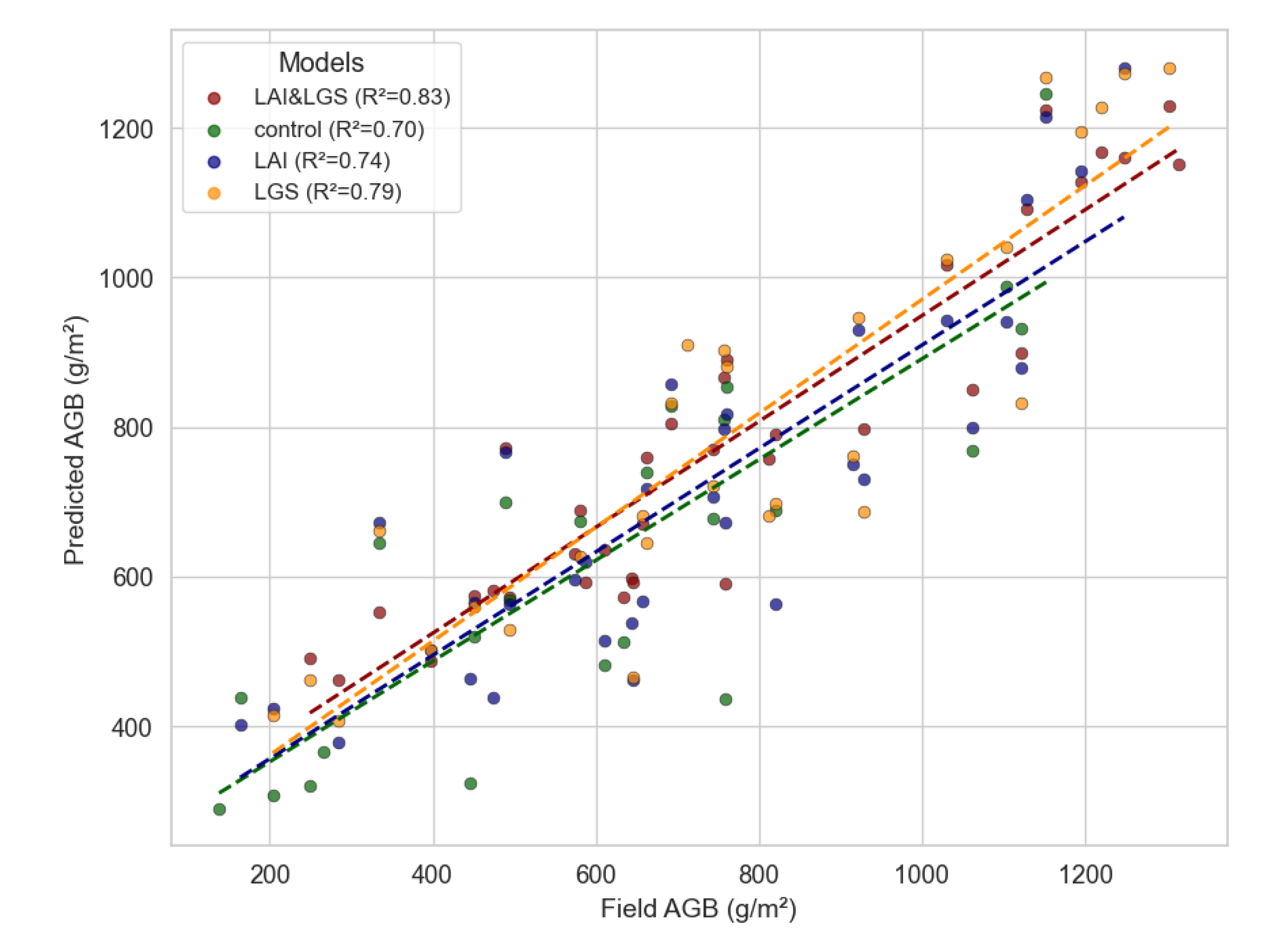
Variable importance analysis in the RF model indicated that both LGS and LAI play an important role in enhancing model performance. To further investigate their effectiveness to AGB estimation, we re-developed the models by sequentially removing these two variables. For a more pronounced comparison, 78 representative sampling sites within the study area were selected for this analysis. By taking the results from model without LAI and LGS as baseline, the incorporation of LAI and LGS individually led to improvements in model accuracy of 5.7% and 12.9%, respectively. The inclusion of LAI effectively mitigated the overestimation observed in high-biomass regions, resulting in a more stable and reliable model. This finding confirms that both variables contribute to improving AGB estimation, which is consistent with previous studies [47,48,49]. Notably, LGS exerted a stronger influence than LAI, which aligns with ecological theory, as the length of the growing season directly relates to the amount of carbon fixed by vegetation. Previous studies have reported that the influence of LGS on biomass is significant in warm regions [12]. The YRD, being a temperate semi-humid area, confirms that phenology has a notable impact on the accuracy of AGB estimation. The current estimation did not include climatic factors such as drought, which has been identified as critical drivers of biomass variability through their influence on water and heat availability [50]. Future studies should investigate the interactions between multiple environments variables and biomass accumulation, with particular attention to plant carbon fixation processes, to further improve the accuracy of AGB estimation.
Figure 10.
Model performance under different scenarios of LAI and LGS inclusion.
5.3. Drivers of AGB Variation in the YRD
The YRD is predominantly covered by herbaceous vegetation and has experienced frequent land cover changes over the past decades. In this study, we focused on the dynamics of cropland, grassland, and wetlands, in order to evaluate their contributions to biomass changes and assess the ecological status of the region. Over the past twenty years, cropland, accounting for 58% of the area has remained relatively stable, whereas grassland, accounting for only 1% and wetlands, which cover 41% of the region, have fluctuated considerably and exhibited an overall declining trend (Figure 11a). For cropland, although its area has remained relatively stable, its total AGB has consistently stayed around or even exceeded 600,000 g C over the years. Moreover, the mean AGB has shown an overall increasing trend over the past two decades, with a slight decline in the most recent five years. This indicates that cropland biomass density has played a dominant role in driving cropland overall AGB variation (Figure 11b). For grassland, both its area and total AGB exhibited a similar declining trend. Although the AGB per unit area has increased, the limited overall area restricts its potential to rapidly restore carbon sequestration capacity through quality improvements alone. Therefore, maintaining grassland area from further encroachment should be a key priority (Figure 11c). For wetlands, the total AGB has generally declined over the past two decades in line with the reduction in wetland area. However, in the past five years, the continuous increase in AGB per unit area has led to a stabilization or even a slight increase in total AGB. Although wetlands have historically been the primary driver of biomass fluctuations in the region, recent environmental protection policies have shown positive effects, resulting in a gradual stabilization of AGB variability associated with wetlands (Figure 11d). These findings suggest that ecological conservation efforts should not only aim to maintain wetland area but also focus on improving wetland quality. The observed area fluctuations and AGB changes also reflect substantial governmental efforts to protect the YRD environment. Previous studies have shown that since 2005, the implementation of twelve water diversion and sediment regulation policies has gradually enhanced freshwater resources in the delta, reducing landscape fragmentation [27]. To achieve a sustainable balance between human development and ecological conservation, future policies should not only prioritize land cover restoration but also implement comprehensive measures to enhance vegetation quality.
6. Conclusions
In this study, we collected 4,717 herbaceous aboveground biomass (AGB) samples through literature-based data synthesizing. By incorporation of leaf area index (LAI) and length of growing season (LGS), along with reflectance, vegetation indices (VIs) and topographic variables, we developed a robust AGB estimation model using the random forest (RF) algorithm. This model was applied to estimate AGB across the Yellow River Delta (YRD) from 2001 to 2022. Subsequently, we analyzed the spatiotemporal dynamics of AGB over the past 22 years and assessed the influence of different land cover types on biomass changes.
The main findings are as follows: (1) The RF model incorporating LAI and LGS outperformed other machine learning algorithms, achieving high estimation accuracy with an R² of 0.74. (2) During 2001 to 2022, the higher biomass was consistently observed in croplands, particularly in the western region, while lower values were concentrated in areas south of the Yellow River, especially in coastal zones. (3) AGB exhibited a fluctuating upward trend from 204.07 g/m² to at 230.79 g/m² during 2007 to 2015. Since 2016, AGB has remained relatively stable, fluctuating between 215 g/m² and 225 g/m², indicating sustained productivity across the region. (4) AGB increased markedly along the main branches of the Yellow River and in intensively cultivated croplands, while coastal zones showed significant declines. (5) Cropland and wetlands were the primary positive drivers of AGB accumulation, with croplands showing stable contributions while wetlands introduced high variability; grasslands had modest and occasionally suppressed effect, collectively shaping the spatial heterogeneity of AGB dynamics.
Overall, this study highlights the importance of integrating ecological variables, which substantially enhance the effectiveness and reliability of AGB estimation in herbaceous-dominated landscapes. The observed spatial expansion and increasing trend of AGB over the past two decades reflect the evolving vegetation productivity in the YRD. However, the heterogeneous responses among different land cover types, especially the instability observed in wetland areas, underscore the complex and sensitive nature of deltaic ecosystems. These findings not only provide a scientific basis for large-scale biomass monitoring and ecological assessment but also offer valuable guidance for land use management and wetland conservation in coastal regions.
Author Contributions
Conceptualization, S.Z. and W.S.; methodology, S.Z., W.S. and N.H.; validation, W.S.; formal analysis, S.Z.; investigation, Y.Z.; resources, L.W.; data curation, C.L. and Y.L.; writing—original draft preparation, S.Z.; writing—review and editing, S.Z., W.S., F.T. and N.H.; visualization, S.Z.; supervision, L.W.; project administration, W.S.; funding acquisition, W.S. and L.W. All authors have read and agreed to the published version of the manuscript.
Funding
This research was funded by the Science & Technology Fundamental Resources Investigation Program under Grant No. 2022FY100302, and the National Natural Science Foundation of China–Geological Joint Fund under Grant No. U2244230.
Data Availability Statement
The original contributions presented in the study are included in the article; further inquires can be directed to the corresponding author.
Conflicts of Interest
The authors declare no conflicts of interest.
References
- Tilman, D.; Wedin, D.; Knops, J. Productivity and Sustainability Influenced by Biodiversity in Grassland Ecosystems. Nature 1996, 379, 718–720. [Google Scholar] [CrossRef]
- Dai, X.; Yang, G.; Liu, D.; Wan, R. Vegetation Carbon Sequestration Mapping in Herbaceous Wetlands by Using a MODIS EVI Time-Series Data Set: A Case in Poyang Lake Wetland, China. Remote Sensing 2020, 12, 3000. [Google Scholar] [CrossRef]
- Chave, J.; Réjou-Méchain, M.; Búrquez, A.; Chidumayo, E.; Colgan, M.S.; Delitti, W.B.C.; Duque, A.; Eid, T.; Fearnside, P.M.; Goodman, R.C.; et al. Improved Allometric Models to Estimate the Aboveground Biomass of Tropical Trees. [CrossRef]
- Zhou, R.; Yang, C.; Li, E.; Cai, X.; Wang, X. Aboveground Biomass Estimation of Wetland Vegetation at the Species Level Using Unoccupied Aerial Vehicle RGB Imagery. Front. Plant Sci. 2023, 14. [Google Scholar] [CrossRef]
- Yang, D.; Yang, Z.; Wen, Q.; Ma, L.; Guo, J.; Chen, A.; Zhang, M.; Xing, X.; Yuan, Y.; Lan, X.; et al. Dynamic Monitoring of Aboveground Biomass in Inner Mongolia Grasslands over the Past 23 Years Using GEE and Analysis of Its Driving Forces. Journal of Environmental Management 2024, 354, 120415. [Google Scholar] [CrossRef]
- Jianlong, L.; Liang, T.; Quangong, C. Estimating Grassland Yields Using Remote Sensing and GIS Technologies in China. New Zealand Journal of Agricultural Research - N Z J AGR RES 1998, 41, 31–38. [Google Scholar] [CrossRef]
- Morais, T.G.; Teixeira, R.F.M.; Figueiredo, M.; Domingos, T. The Use of Machine Learning Methods to Estimate Aboveground Biomass of Grasslands: A Review. Ecological Indicators 2021, 130, 108081. [Google Scholar] [CrossRef]
- Boussetta, S.; Balsamo, G.; Beljaars, A.; Kral, T.; Jarlan, L. Impact of a Satellite-Derived Leaf Area Index Monthly Climatology in a Global Numerical Weather Prediction Model. International Journal of Remote Sensing 2013, 34, 3520–3542. [Google Scholar] [CrossRef]
- Fang, H.; Baret, F.; Plummer, S.; Schaepman-Strub, G. An Overview of Global Leaf Area Index (LAI): Methods, Products, Validation, and Applications. Reviews of Geophysics 2019, 57, 739–799. [Google Scholar] [CrossRef]
- Yuan, W.; Meng, Y.; Li, Y.; Ji, Z.; Kong, Q.; Gao, R.; Su, Z. Research on Rice Leaf Area Index Estimation Based on Fusion of Texture and Spectral Information. Computers and Electronics in Agriculture 2023, 211, 108016. [Google Scholar] [CrossRef]
- Tian, J.; Luo, X.; Xu, H.; Green, J.K.; Tang, H.; Wu, J.; Piao, S. Slower Changes in Vegetation Phenology than Precipitation Seasonality in the Dry Tropics. Global Change Biology 2024, 30, e17134. [Google Scholar] [CrossRef]
- MacDougall, A.S.; Esch, E.; Chen, Q.; Carroll, O.; Bonner, C.; Ohlert, T.; Siewert, M.; Sulik, J.; Schweiger, A.K.; Borer, E.T.; et al. Widening Global Variability in Grassland Biomass since the 1980s. Nat Ecol Evol 2024, 8, 1877–1888. [Google Scholar] [CrossRef]
- Morais, T.G.; Teixeira, R.F.M.; Figueiredo, M.; Domingos, T. The Use of Machine Learning Methods to Estimate Aboveground Biomass of Grasslands: A Review. Ecological Indicators 2021, 130, 108081. [Google Scholar] [CrossRef]
- Li, H.; Liu, K.; Yang, B.; Wang, S.; Meng, Y.; Wang, D.; Liu, X.; Li, L.; Li, D.; Bo, Y.; et al. Continuous Monitoring of Grassland AGB during the Growing Season through Integrated Remote Sensing: A Hybrid Inversion Framework. International Journal of Digital Earth 2024, 17. [Google Scholar] [CrossRef]
- Wang, J.; Xiao, X.; Bajgain, R.; Starks, P.; Steiner, J.; Doughty, R.B.; Chang, Q. Estimating Leaf Area Index and Aboveground Biomass of Grazing Pastures Using Sentinel-1, Sentinel-2 and Landsat Images. ISPRS Journal of Photogrammetry and Remote Sensing 2019, 154, 189–201. [Google Scholar] [CrossRef]
- Wang, S.; Tuya, H.; Zhang, S.; Zhao, X.; Liu, Z.; Li, R.; Lin, X. Random Forest Method for Analysis of Remote Sensing Inversion of Aboveground Biomass and Grazing Intensity of Grasslands in Inner Mongolia, China. International Journal of Remote Sensing 2023, 44, 2867–2884. [Google Scholar] [CrossRef]
- Zeng, C.; Wu, J.; Zhang, X. Effects of Grazing on Above- vs. Below-Ground Biomass Allocation of Alpine Grasslands on the Northern Tibetan Plateau. PLOS ONE 2015, 10, e0135173. [Google Scholar] [CrossRef]
- Using the Random Forest Model and Validated MODIS with the Field Spectrometer Measurement Promote the Accuracy of Estimating Aboveground Biomass and Coverage of Alpine Grasslands on the Qinghai-Tibetan Plateau. Ecological Indicators 2020, 112, 106114. [CrossRef]
- Breiman, L. Random Forests. Machine Learning 2001, 45, 5–32. [Google Scholar] [CrossRef]
- Li, H.; Li, F.; Xiao, J.; Chen, J.; Lin, K.; Bao, G.; Liu, A.; Wei, G. A Machine Learning Scheme for Estimating Fine-Resolution Grassland Aboveground Biomass over China with Sentinel-1/2 Satellite Images. Remote Sensing of Environment 2024, 311, 114317. [Google Scholar] [CrossRef]
- Wu, J.; Li, Y.; Li, N.; Shi, P. Development of an Asset Value Map for Disaster Risk Assessment in China by Spatial Disaggregation Using Ancillary Remote Sensing Data. Risk Analysis 2018, 38, 17–30. [Google Scholar] [CrossRef]
- Zhang, C.; Zhao, L.; Zhang, H.; Chen, M.; Fang, R.; Yao, Y.; Zhang, Q.; Wang, Q. Spatial-Temporal Characteristics of Carbon Emissions from Land Use Change in Yellow River Delta Region, China. Ecological Indicators 2022, 136, 108623. [Google Scholar] [CrossRef]
- Hall Cushman, J.; Waller, J.C.; Hoak, D.R. Shrubs as Ecosystem Engineers in a Coastal Dune: Influences on Plant Populations, Communities and Ecosystems: Shrubs as Mediators of a Coastal Dune. Journal of Vegetation Science 2010, 21, 821–831. [Google Scholar] [CrossRef]
- Ma, W.; Fang, J.; Yang, Y.; Mohammat, A. Biomass Carbon Stocks and Their Changes in Northern China’s Grasslands during 1982–2006. Sci. China Life Sci. 2010, 53, 841–850. [Google Scholar] [CrossRef]
- Fu, W.; Huang, M.; Horton, R. Soil Carbon Dioxide (CO2) Efflux of Two Shrubs in Response to Plant Density in the Northern Loess Plateau of China. African Journal of Biotechnology 2010, 9, 6916–6926. [Google Scholar]
- The Effect of Land Use and Land Cover on Soil Carbon Storage in the Yellow River Delta, China: Implications for Wetland Restoration and Adaptive Management. Journal of Environmental Management 2024, 367, 122097. [CrossRef]
- Zhang, X.; Wang, G.; Xue, B.; Zhang, M.; Tan, Z. Dynamic Landscapes and the Driving Forces in the Yellow River Delta Wetland Region in the Past Four Decades. Science of The Total Environment 2021, 787, 147644. [Google Scholar] [CrossRef] [PubMed]
- Xu, Z.; Li, R.; Dou, W.; Wen, H.; Yu, S.; Wang, P.; Ning, L.; Duan, J.; Wang, J. Plant Diversity Response to Environmental Factors in Yellow River Delta, China. Land 2024, 13, 264. [Google Scholar] [CrossRef]
- Xu, T.; Wang, F.; Shi, Z.; Xie, L.; Yao, X. Dynamic Estimation of Rice Aboveground Biomass Based on Spectral and Spatial Information Extracted from Hyperspectral Remote Sensing Images at Different Combinations of Growth Stages. ISPRS Journal of Photogrammetry and Remote Sensing 2023, 202, 169–183. [Google Scholar] [CrossRef]
- Anselin, L. Local Indicators of Spatial Association—LISA. Geographical Analysis 1995, 27, 93–115. [Google Scholar] [CrossRef]
- Summary of Current Radiometric Calibration Coefficients for Landsat MSS, TM, ETM+, and EO-1 ALI Sensors. Remote Sensing of Environment 2009, 113, 893–903. [CrossRef]
- Vermote, E.F.; Tanre, D.; Deuze, J.L.; Herman, M.; Morcette, J.-J. Second Simulation of the Satellite Signal in the Solar Spectrum, 6S: An Overview. IEEE Transactions on Geoscience and Remote Sensing 1997, 35, 675–686. [Google Scholar] [CrossRef]
- Masek, J.G.; Vermote, E.F.; Saleous, N.E.; Wolfe, R.; Hall, F.G.; Huemmrich, K.F.; Gao, F.; Kutler, J.; Lim, T.-K. A Landsat Surface Reflectance Dataset for North America, 1990-2000. IEEE Geoscience and Remote Sensing Letters 2006, 3, 68–72. [Google Scholar] [CrossRef]
- Skakun, S.; Vermote, E.F.; Roger, J.-C.; Justice, C.O.; Masek, J.G. Validation of the LaSRC Cloud Detection Algorithm for Landsat 8 Images. IEEE Journal of Selected Topics in Applied Earth Observations and Remote Sensing 2019, 12, 2439–2446. [Google Scholar] [CrossRef]
- Berk, A.; Conforti, P.; Kennett, R.; Perkins, T.; Hawes, F.; van den Bosch, J. MODTRAN® 6: A Major Upgrade of the MODTRAN® Radiative Transfer Code. In Proceedings of the 2014 6th Workshop on Hyperspectral Image and Signal Processing: Evolution in Remote Sensing (WHISPERS); June 2014; pp. 1–4. [Google Scholar]
- Wang, C.; Chen, J.; Wu, J.; Tang, Y.; Shi, P.; Black, T.A.; Zhu, K. A Snow-Free Vegetation Index for Improved Monitoring of Vegetation Spring Green-up Date in Deciduous Ecosystems. Remote Sensing of Environment 2017, 196, 1–12. [Google Scholar] [CrossRef]
- Baret, F.; Jacquemoud, S.; Hanocq, J.F. The Soil Line Concept in Remote Sensing. Remote Sensing Reviews 1993, 7, 65–82. [Google Scholar] [CrossRef]
- Zhang, X.; Liu, L.; Chen, X.; Gao, Y.; Xie, S.; Mi, J. GLC_FCS30: Global Land-Cover Product with Fine Classification System at 30 m Using Time-Series Landsat Imagery. Earth System Science Data 2021, 13, 2753–2776. [Google Scholar] [CrossRef]
- Ali, I.; Cawkwell, F.; Dwyer, E.; Green, S. Modeling Managed Grassland Biomass Estimation by Using Multitemporal Remote Sensing Data—A Machine Learning Approach. IEEE Journal of Selected Topics in Applied Earth Observations and Remote Sensing 2016, 10, 3254–3264. [Google Scholar] [CrossRef]
- Clevers, J.G.P.W.; van der Heijden, G.W.A.M.; Verzakov, S.; Schaepman, M.E. Estimating Grassland Biomass Using SVM Band Shaving of Hyperspectral Data. Photogrammetric Engineering & Remote Sensing 2007, 73, 1141–1148. [Google Scholar] [CrossRef]
- Fensholt, R.; Rasmussen, K.; Nielsen, T.T.; Mbow, C. Evaluation of Earth Observation Based Long Term Vegetation Trends — Intercomparing NDVI Time Series Trend Analysis Consistency of Sahel from AVHRR GIMMS, Terra MODIS and SPOT VGT Data. Remote Sensing of Environment 2009, 113, 1886–1898. [Google Scholar] [CrossRef]
- Yue, S.; Wang, C. The Mann-Kendall Test Modified by Effective Sample Size to Detect Trend in Serially Correlated Hydrological Series. Water Resources Management 2004, 18, 201–218. [Google Scholar] [CrossRef]
- Su, B.; Ang, B.W. Structural Decomposition Analysis Applied to Energy and Emissions: Some Methodological Developments. Energy Economics 2012, 34, 177–188. [Google Scholar] [CrossRef]
- Estimation of Biomass in Wheat Using Random Forest Regression Algorithm and Remote Sensing Data. The Crop Journal 2016, 4, 212–219. [CrossRef]
- Gough, L.; Moore, J.C.; Shaver, G.R.; Simpson, R.T.; Johnson, D.R. Above- and Belowground Responses of Arctic Tundra Ecosystems to Altered Soil Nutrients and Mammalian Herbivory. Ecology 2012, 93, 1683–1694. [Google Scholar] [CrossRef]
- Rigueiro-Rodríguez, A.; Mouhbi, R.; Santiago-Freijanes, J.J.; González-Hernández, M.D.P.; Mosquera-Losada, M.R. Horse Grazing Systems: Understory Biomass and Plant Biodiversity of a Pinus Radiata Stand. Sci. agric. (Piracicaba, Braz.) 2012, 69, 38–46. [Google Scholar] [CrossRef]
- Dusseux, P.; Hubert-Moy, L.; Corpetti, T.; Vertès, F. Evaluation of SPOT Imagery for the Estimation of Grassland Biomass. International Journal of Applied Earth Observation and Geoinformation 2015, 38, 72–77. [Google Scholar] [CrossRef]
- Xie, J.; Wang, C.; Ma, D.; Chen, R.; Xie, Q.; Xu, B.; Zhao, W.; Yin, G. Generating Spatiotemporally Continuous Grassland Aboveground Biomass on the Tibetan Plateau Through PROSAIL Model Inversion on Google Earth Engine. IEEE Transactions on Geoscience and Remote Sensing 2022, 60, 1–10. [Google Scholar] [CrossRef]
- Diverse and Divergent Influences of Phenology on Herbaceous Aboveground Biomass across the Tibetan Plateau Alpine Grasslands. Ecological Indicators 2021, 121, 107036. [CrossRef]
- Spatiotemporal Analysis of AGB and BGB in China: Responses to Climate Change under SSP Scenarios. Geoscience Frontiers 2025, 16, 102038. [CrossRef]
Figure 1.
Raw biomass distribution and log-Transformed distribution. The log-transformed AGB values are dimensionless because the logarithmic transformation removes units.
Figure 1.
Raw biomass distribution and log-Transformed distribution. The log-transformed AGB values are dimensionless because the logarithmic transformation removes units.
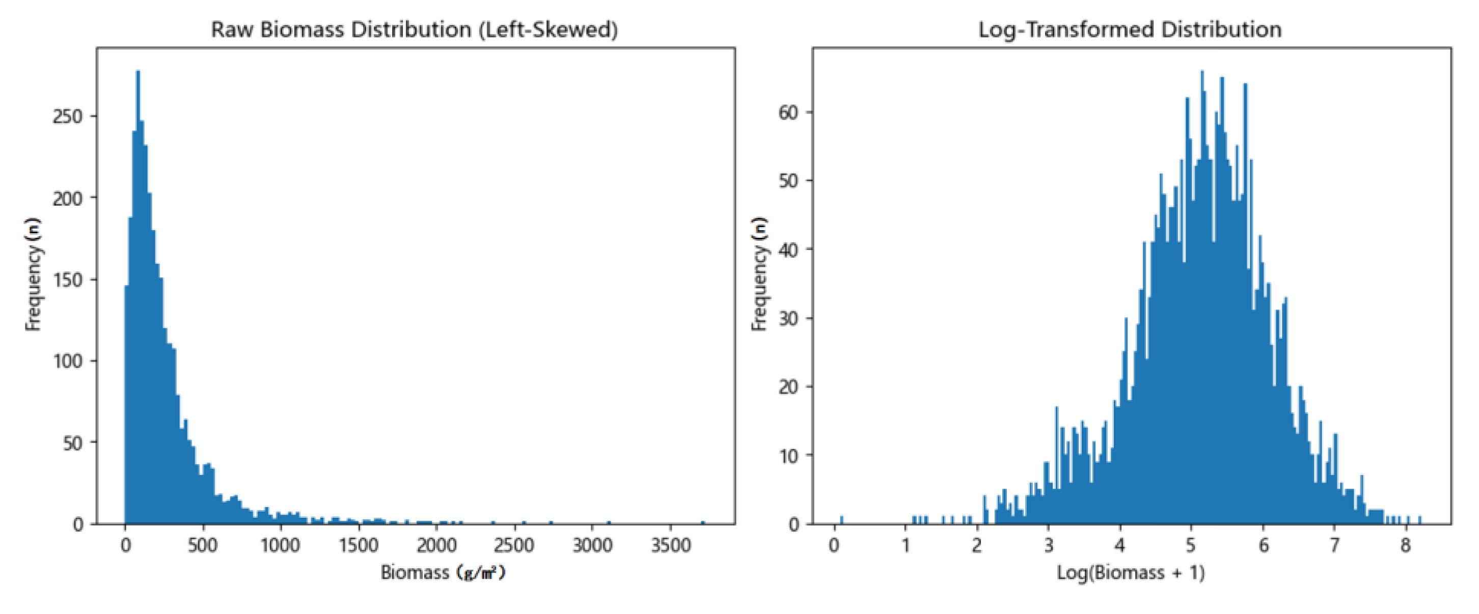
Figure 2.
Land cover of YRD in 2020.
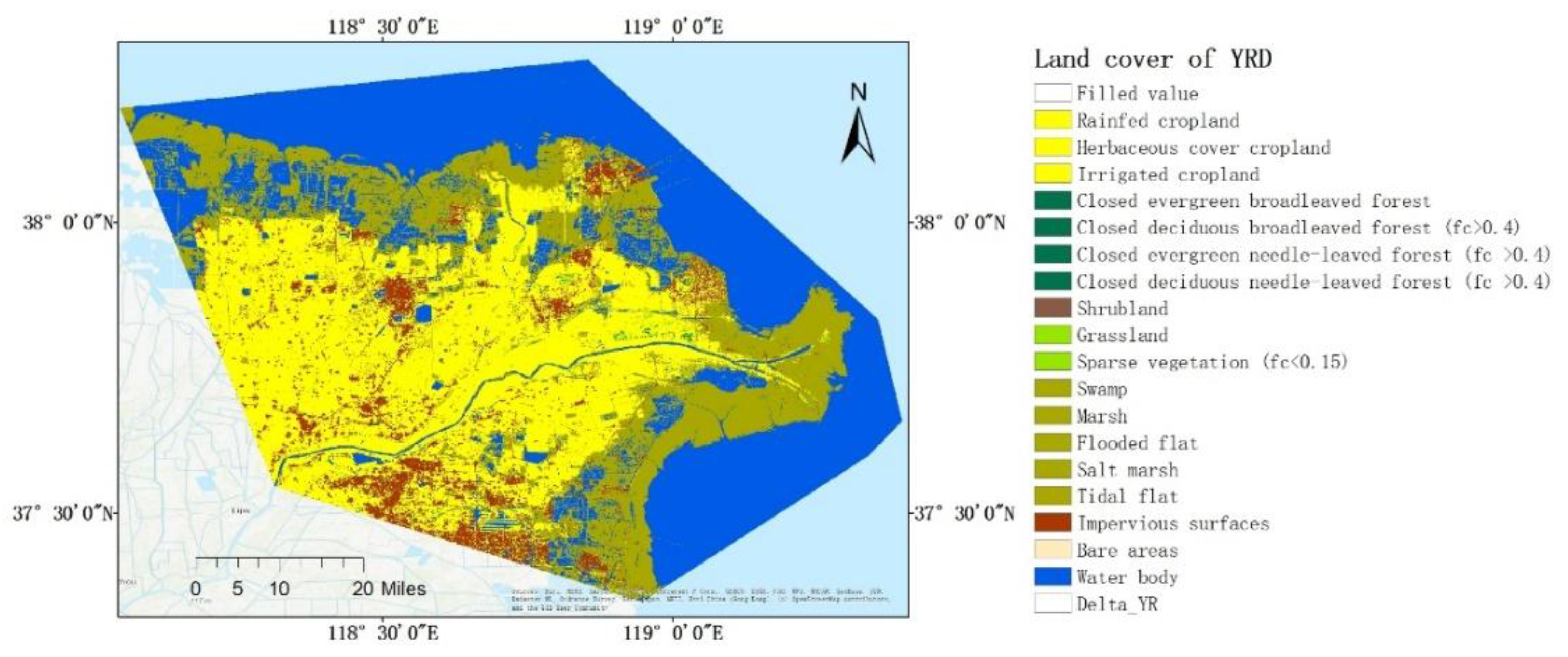
Figure 3.
Variables importance of RF model.
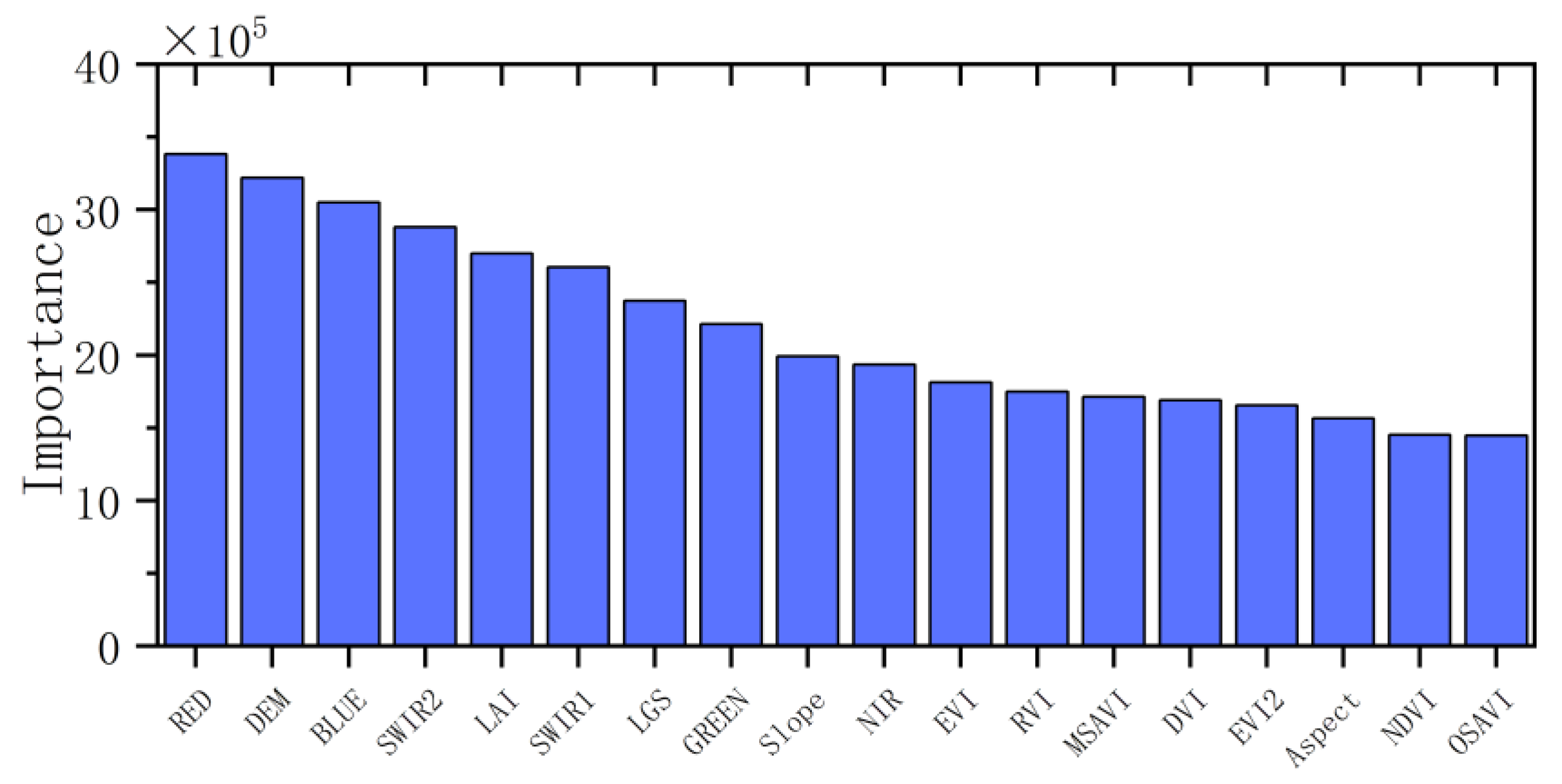
Figure 4.
Spatial distribution of herbaceous AGB in YRD from 2001 to 2020. (a) AGB in 2001. (b) AGB in 2005. (c) AGB in 2010. (d) AGB in 2015. (e) AGB in 2020. (f) Multi-year average AGB.
Figure 4.
Spatial distribution of herbaceous AGB in YRD from 2001 to 2020. (a) AGB in 2001. (b) AGB in 2005. (c) AGB in 2010. (d) AGB in 2015. (e) AGB in 2020. (f) Multi-year average AGB.
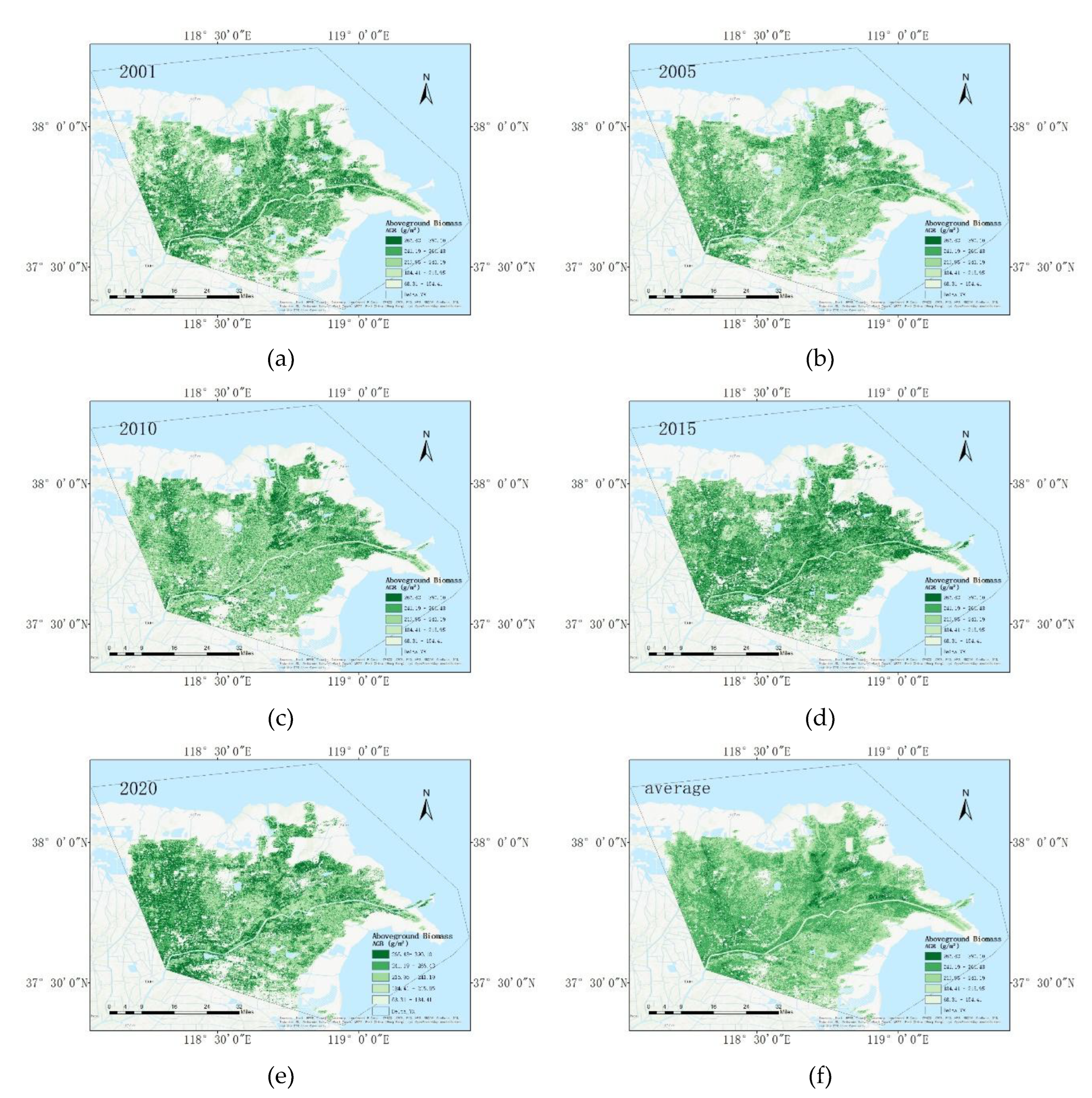
Figure 5.
Annual average AGB in the YRD from 2001 to 2022.
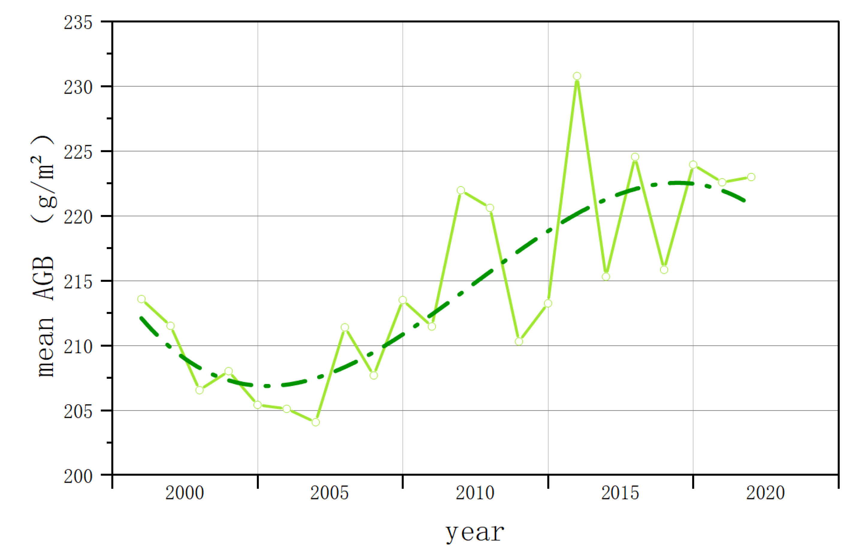
Figure 6.
The spatial distribution of the annual maximum AGB change trend in YRD (2001-2022).
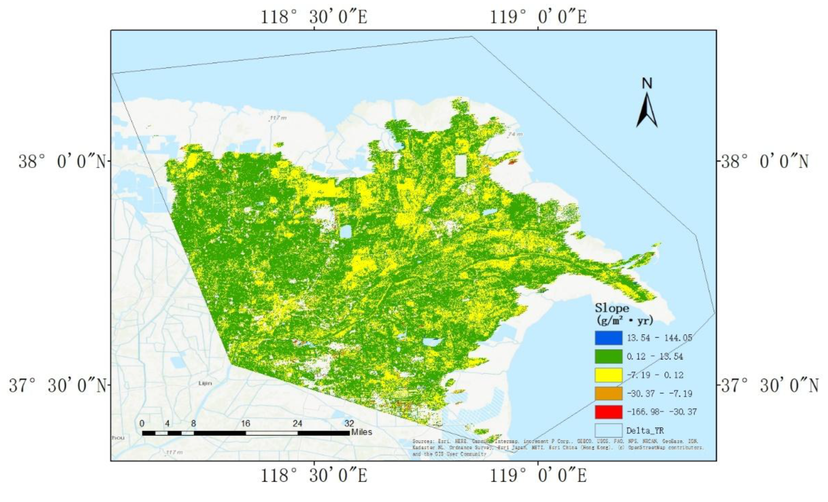
Figure 7.
The trend significance of AGB changes in YRD (2001-2022).
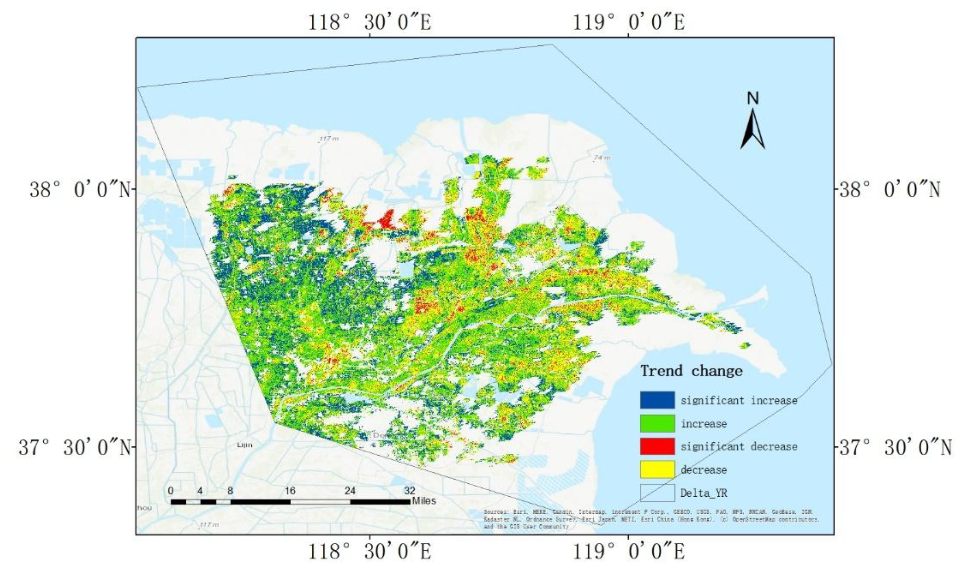
Figure 8.
Contributions of land cover to AGB changes in YRD (2001-2022). Higher values indicate higher contributions to AGB changes, positive values represent contributions to AGB increases, and negative values represent contributions to AGB reduction.
Figure 8.
Contributions of land cover to AGB changes in YRD (2001-2022). Higher values indicate higher contributions to AGB changes, positive values represent contributions to AGB increases, and negative values represent contributions to AGB reduction.
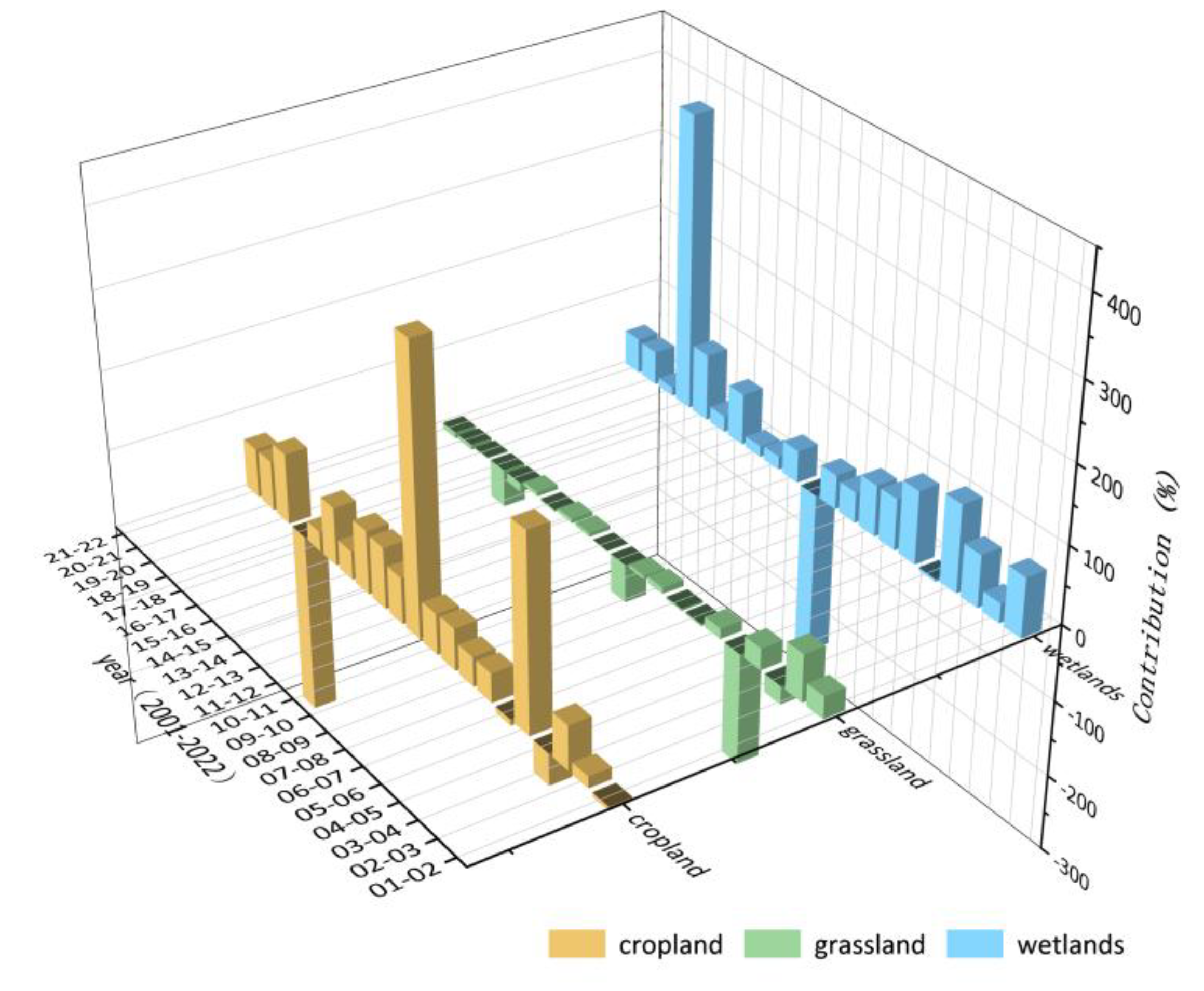
Figure 9.
Area, density and interaction effect of land cover types on AGB changes in YRD (2001-2022). Area effect refers to the influence of changes in land cover area on AGB changes; density effect refers to the influence of changes in AGB density on AGB changes; and interaction effect refers to the combined impact of area and density changes acting together on AGB changes.
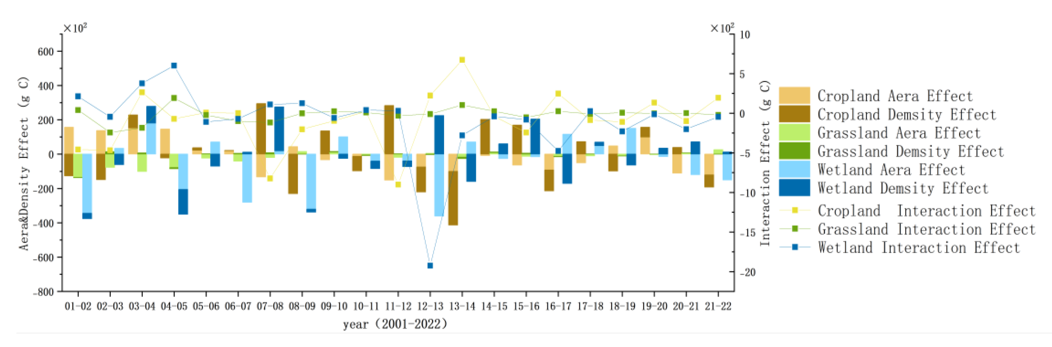
Figure 11.
Land cover area and AGB changes in the YRD from 2001 to 2022. (a). Land cover area changes. (b). Cropland AGB changes. (c). Grassland AGB changes. (d). Wetlands AGB changes.
Figure 11.
Land cover area and AGB changes in the YRD from 2001 to 2022. (a). Land cover area changes. (b). Cropland AGB changes. (c). Grassland AGB changes. (d). Wetlands AGB changes.
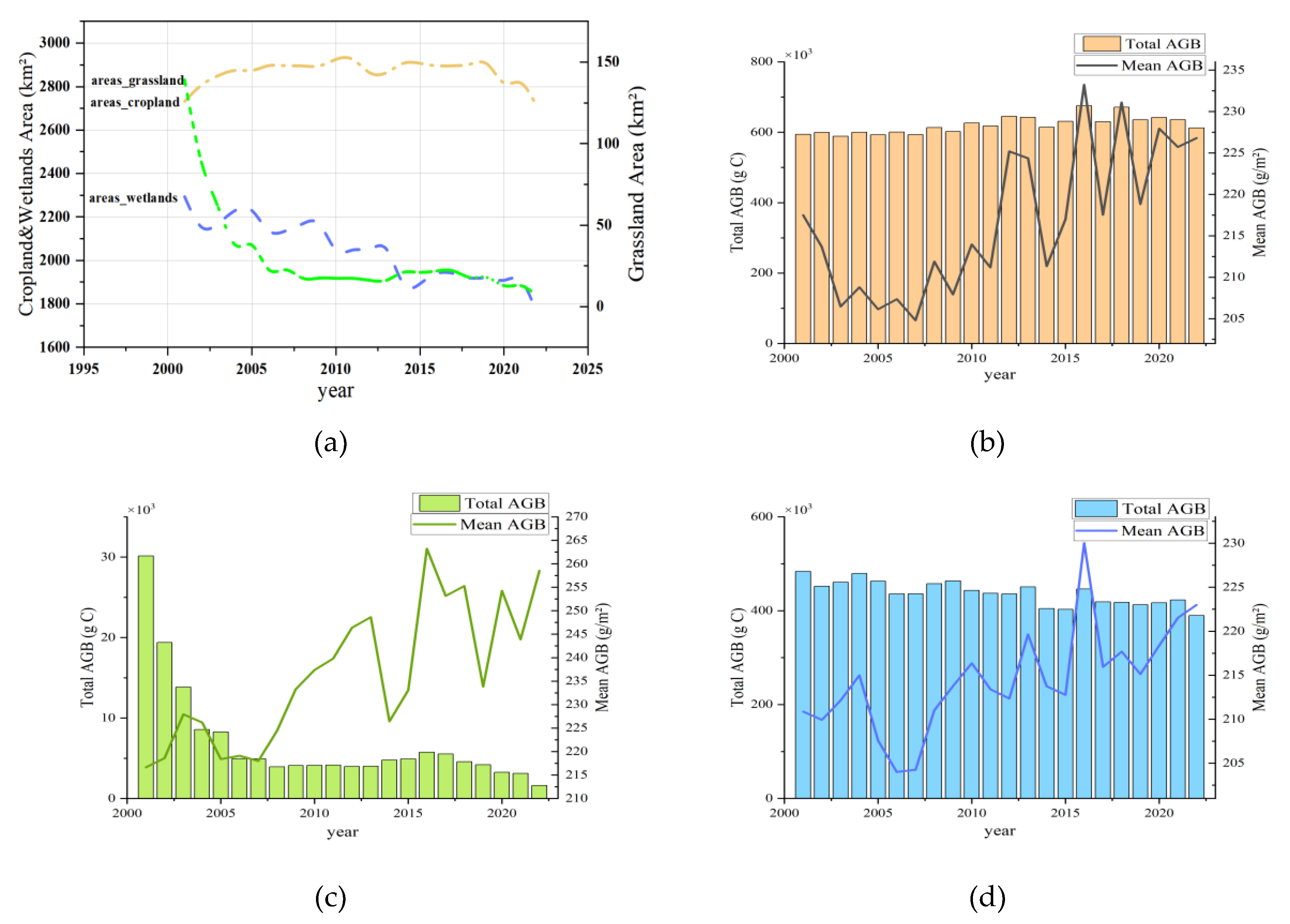

Table 1.
AGB estimated VIs and formula.
| VIs | Formula |
| RVI | |
| EVI | |
| DVI | |
| NDVI | |
| NDPI | |
| MSAVI | |
| OSAVI |
Table 2.
Reclassified land cover.
| Reclassified Land Cover | GLC-FCS30 |
| Cropland | Herbaceous cover cropland, Rainfed cropland, Irrigated cropland; |
| Grassland | Grassland, Lichens and mosses, Sparse herbaceous (fc<0.15); |
| Wetlands | Swamp, Marsh, Flooded flat, Salt marsh, Tidal flat; |
Table 3.
Feature categories and variables.
| Feature categories | Variables |
| spectral variables | BLUE, GREEN, RED, NIR, SWIR1, SWIR2; |
| vegetation indices | NDVI, EVI, EVI2, RVI, DVI, OSAVI, MSAVI; |
| topographic variables | Elevation, Slope, Aspect; |
| ecological variables | LAI, LGS; |
Table 4.
Accuracy assessment of three models.
| Model | R² | RMSE(g/m²) | Precision (%) |
| RF | 0.74 | 77.13 | 88.07% |
| SVM | 0.67 | 137.33 | 80.63% |
| ANN | 0.55 | 224.75 | 85.96% |
Disclaimer/Publisher’s Note: The statements, opinions and data contained in all publications are solely those of the individual author(s) and contributor(s) and not of MDPI and/or the editor(s). MDPI and/or the editor(s) disclaim responsibility for any injury to people or property resulting from any ideas, methods, instructions or products referred to in the content. |
© 2025 by the authors. Licensee MDPI, Basel, Switzerland. This article is an open access article distributed under the terms and conditions of the Creative Commons Attribution (CC BY) license (http://creativecommons.org/licenses/by/4.0/).
Copyright: This open access article is published under a Creative Commons CC BY 4.0 license, which permit the free download, distribution, and reuse, provided that the author and preprint are cited in any reuse.


