
Submitted:
21 August 2025
Posted:
26 August 2025
You are already at the latest version
Abstract
In this study, thermal properties (thermal diffusivity, thermal conductivity, damping depth, thermal effusivity, heat wave velocity, heat wave length and heat heat flux) were calculated using various classical (amplitude, arctangent, logarithmic, phase) and improved (point) models in winter, spring, summer and fall in alkaline and non-alkaline soil. For this purpose, temperature sensors were placed at different depths (0, 5, 10, 15, 20, 40 cm) on non-alkaline and alkaline lands, and temperature data were collected from the sensors for 365 days. The study showed that (i) the thermal properties of both soils vary depending on the seasons of the year, and (ii) the thermal properties (thermal conductivity, thermal conductivity coefficient, thermal conductivity, attenuation depth, thermal conductivity coefficient, speed and length of the heat wave) were lower in alkaline soil. The result coul be used for consideration of climate change mitigationin in similar semi-arid zone.
Keywords:
Soil
; thermal diffusivity
; thermal conductivity
; alkalinity
; modelling
; seasons
; improved method
1. Introduction
In soil formation, climate, topography, parent material and organisms outstand as effective factors. Soil salinity or alkalinity, which is caused by the effects of climate,topography and anthropogenic factors, is one of the important problems of arid-semi-arid regions and has negative effects on soil health [1,2].
Soil temperature, in the context of climate change may affect soil functioning and quality, which is one of the important factors of climate, is effective on physical (soil thermal properties, water flow etc.), chemical (mineralization, nutrients etc.) and biological (microbial activity, microbial community etc.) properties of soils [3,4,5]. Soil thermal properties are closely related to moisture content, temperature, bulk density, organic matter, salt content and porosity [5]. Some researchers have determined that in non-sodic soils, as the salt content of the soils increases, the thermal diffusivity decreases. In sodic soils sSodicity (ESP), which refers to the presence of excessive sodium ions (Na⁺) in the soil exchange complex, can significantly alter soil structure and behavior, which in turn influences how heat or water are stored and transferred through the soil[1,6,7,8].
Noborio & McInnes (1993) [8] reported that the apparent thermal conductivity of soils decreases as the salt concentration increases. Abu-Hamdeh & Reeder (2000) [9,10] also detected that an increase in the amount of added salts, at a given moisture content, decreased thermal conductivity. Morozova [11] determined that the thermal conductivity increased with the increase of KCl. Tikhonravova [12,13] revealed that the thermaldiffusivity depends not only on the salt content but also on the moisture content.
Relevant research has shown that the field studies cost money, labor, time, etc. in determining the thermal properties of the soils. This shows that laboratory measurements under controlled conditions and in shorter periods are common [14,15,16,17,18].
Although the effects of salts on thermal properties of soils have been studied, these studies were carried out under controlled conditions in the laboratory and may not reflect the field conditions, particularly for sodic or alkline soils[]`. In field conditions, it is important to calculate thermal properties with long-term temperature measurements ot the main thermal properties of soils such as volumetric heat capacity (Cv), thermal diffusivity (κ), thermal conductivity (λ), damping depth (d), thermal effusivity (e), heat wave velocity (υ), heat wave length (Λ) and heat flow (q).
The determination of these parameters is important in shaping the thermal regimes of soils. In this work, classical (amplitude, arctangent, logarithmic, and phase) methods are first used to determine the thermal conductivity coefficient [19,20,21,22,23,24,25,26,27,28,29,30,31]. Subsequently, a new "point" method was developed by our team [32,33,34,35,36,37,38], which, unlike classical approaches, also incorporates the amplitude of daily surface soil temperature (Ta)—a critical parameter that significantly influences thermal diffusivity in soils. Moreover, the proposed method accounts for the depth of the soil profile (i.e., z = L). Notably, in this approach, the thermal diffusivity parameter can be calculated at any investigation point (zi) within the soil profile. Selecting the most suitable predictive model is essential for the effective monitoring and management of soil thermal dynamics. Accurate models provide deeper insight into soil temperature fluctuations, which directly influence key processes such as irrigation scheduling, crop development, nutrient cycling, and microbial activity. Reliable predictions of soil thermal properties are particularly valuable for informed decision-making in areas such as precision agriculture, land reclamation, and environmental monitoring. Consequently, evaluating and selecting models based on their accuracy and performance under real field conditions is critical to promoting long-term sustainability and efficient resource use. [3-5, 9, 10, fm32-38].
he objectives of this study were: (i) to calculate thermal diffusivity (κ) using both classical methods and the new "point" method developed by our team, and to identify the most accurate method for the study area; (ii) to determine key thermal properties of the soil—namely volumetric heat capacity (Cv), thermal diffusivity (κ), thermal conductivity (λ), damping depth (d), thermal effusivity (e), heat wave velocity (υ), heat wavelength (Λ), and heat flow (Q)—across different seasons; and (iii) to investigate the effect of soil alkalinity on these thermal properties.
2. Mathematical formulation of the problem
The propagation of heat waves in soil represents one of the earliest applications of Fourier's theory of heat conduction [19] to the study of natural phenomena. Numerous theoretical and experimental studies have since been conducted—both in the field and under laboratory conditions—using measured soil temperature data and various heat transfer models to determine the thermal properties of soils. In most of these studies, analytical solutions were derived based on the unrealistic boundary condition T(z→∞,t)=T0T(z \rightarrow \infty, t) = T_0T(z→∞,t)=T0, assuming a constant temperature at an infinite soil depth. Algorithms developed from these solutions have been widely used to estimate the thermal diffusivity parameter.
In contrast, the present study employs analytical solutions that are based on more realistic boundary conditions: this study uses analytical solutions obtained for the boundary conditions ∂T(z=L, t)/∂z=0 at finite (i.e.: z=L) depth and ∂T(∞, t)/∂z=0 at indefinite (i.e.: z→∞) depth, which reflects reality [35,36,37,38].
2.1. The equation of heat movement in soil by conduction
The differential equation that describes the heat movement occurring through conduction in a three-dimensional heterogeneous-isotropic porous medium is expressed as follows [23,24,26,27]:
where T(x,y,z, t) - is the soil temperature (K or °C) at point z (m) at time moment t (sec); ∂T/∂x, ∂T/∂y, ∂T/∂z - is the temperature change in the direction of the ox, oy and, oz axis; ∂T/∂t - is the temperature change in unit time; ρs - is the soil bulk density (kg m-3); cs is the specific heat capacity (J kg-1 °C-1); λx λy λz – is the component of the thermal conductivity of the soil in the x, y and z directions, respectively (Wm-1 °C-1); r - the source of heat inside the soil is (°C).
Experiments have shown that ∂ρs/∂T~0, ∂Cs/∂T~0, ∂λ/∂T~0 are correct for the important soil properties: density, volumetric heat capacity and thermal conductivity parameters when the temperature ranges from -50 ≤ T ≤ + 50 ºC [26, p. 13].
The general one-dimensional heat transfer equation for a homogeneous isotropic porous medium can be written as follows:
where T(z, t) - is the soil temperature (°C) at point z (m) at time moment t (sec); ∂T/∂z - is the temperature change in the direction of the oz axis; ∂T/∂t - is the temperature change in unit time; ρs - is the soil bulk density (kg m-3); cs is the specific heat capacity (J kg-1 °C-1); λz – is the component of the thermal conductivity of the soil in the z direction (Wm-1 °C-1); r - the source of heat inside the soil is (°C).
It is known that when modeling soil processes occurring in the soil-plant-atmosphere system, the main stages are identification (selection of equations describing these processes and boundary conditions) and realization implementation (solution of direct and inverse problems) of the model
Therefore, a systematic approach to analyzing the thermal regime of soil (depending on laboratory or field conditions) should sometimes involve simplification of the heat transfer equation and boundary conditions [36].
Essential simplification of equation (1) is possible for some problems if the coefficients of heat capacity, thermal conductivity and thermal diffusivity of soil are set constant
It is known that one-dimensional heat transfer in soil is described by the classical thermal conductivity equation, which has the form [19,20,21,22,23,24,25,26,27,28,29,30,31,32,33,34,35,36,37,38,39,40,41]:
where T(z, t) is the soil temperature (°C) at point z(m) at time t – time (hour, day, year); κ – thermal diffusivity of the soil (m2 s-1); λ – is the thermal conductivity of the soil (Wm-1 °C-1); Cv = ρs cs – volumetric heat capacity of the soil (J m-3 °C-1); ρs - is the soil bulk density (kg m-3); and cs - is the specific heat capacity (J kg-1 °C-1); L is soil depth (m) starting from which T(z, t) = const or ∂T(L, t)/∂z = 0.
There are a number of works [19,20,21,23,24,25] in which solutions of the heat conduction equation (2.3) under different boundary conditions are considered. In this work we will also consider equation (2.3). In order to determine the change in soil temperature under the influence of various environmental factors depending on a time and depth, equation (1) must be solved analytically or numerically. For this purpose, Equation (1) must be defined and supplemented with initial and boundary conditions that account for the various factors influencing temperature variations in soils.
2.3. Identification boundary-value conditions of the soil heat conduction equation
To solve Equation (2.3) analytically, it is necessary to define initial and boundary conditions that accurately reflect heat transfer within the soil. Depending on the nature of these conditions, three types of initial-boundary value problems can be distinguished.
2.3.1. Identification ınitial condition
It should be noted that, regardless of dimensionality, only one initial condition is required for the thermal conductivity problem because Equation (2.3) is first-order in time (it involves the first derivative of temperature with respect to time). To study the influence of boundary conditions on heat transfer modeling in soil, both initial and boundary conditions must be specified. The temperature distribution of the soil profile at the initial time is given by the following equation, which serves as the initial condition:
Here, φ(z) is the function expressing the distribution of temperature values in the [0, L] or [0,∞) region of the soil.
For modeling, the analytical expression of this function needs to be determined in advance. Some researchers define the function φ(z) as follows:
For convenience of solving the boundary value problem, the function φ(z) is sometimes approximated by a polynomial of degree n. Then the initial condition (2.4) will have the form:
Here an are the coefficients of the polynomial.
It is easy to see that the special case (2.6) for n = 0 corresponds to the uniform initial condition (2.5).
Since the temperature in the soil decreases with depth, the function φ(z) is sometimes approximated by a decreasing step function:
It is known that the influence of the initial condition practically does not affect the soil temperature distribution at the moment of observation.
If the moment of time we are interested in is sufficiently distant from the initial one, it makes sense to neglect the initial conditions, since their influence on the process with the passage of time weakens even more, especially in the case of periodic formulation of the problem. In the periodic formulation of the problem, the initial condition does not need to be given (the so-called “tasks without an initial conditions”) [23,24,25,26,35,36].
2.3.2. Identification of boundary conditions
The condition known as Boundary Condition 1, which expresses the temperature change at the soil surface, is written as a function of time in the following form:
where φ(t) is a function of the soil surface temperature; the analytical form of the function must be determined in advance.
Various empirical functions can be determined by the least squares method (LSM) to analytically express φ(t) based on daily, monthly, or annual soil surface temperature measurements.
As is known, the temperature of the earth has a distinct periodic character, both daily and annual. Sometimes there may be deviations from this periodic distribution.
For example, if the weather is cloudy, the periodicity of the measurement values of the thermal sensors used to determine the temperature values will be disturbed.
In these and similar meteorological (extreme wind, rain, etc.) conditions, periodicity will be disturbed in the distribution of temperature values measured by sensors on the soil surface at some moments of time.
To overcome this deficiency, it is appropriate to use a trigonometric polynomial to determine the analytical expression of the distribution of soil surface temperature values. That is, the first type of boundary condition on the soil surface will be as follows [23,24]:
where T0 is the average daily (or annual) temperature of the active soil surface (oC); Tj is the amplitude of the wave at the surface level for the jth harmonic (oC or K); j is the index of the harmonic in the series; m is the harmonic number; ω = 2π/τ0 is the angular daily (or annual) frequency; τo is the temperature wave period (days or years), for τ0=24 hours: ω = 7,27∙10-5 (rad/s); t – time; εj is the phase angle of the wave at the surface level for the jth harmonic (radians).
Sometimes condition (2.9) can be written in a more practical form:
Here, the parameters T0, Ta, Aj and Bj are calculated by the following formulas:
Where; T(0, ti) - is the temperature of the soil surface at time ti (oC); ti - is the time of observations, N - is the number of observations. The phase shifts (phase angle) εj and amplitude terms (Tj) are calculated with the coefficients Aj and Bj as follows:
The boundary conditions can be set at any depth of the profile, similar to the boundary condition at the soil surface.
The oscillation of the soil temperature wave becomes increasingly relaxed as depth increases, and after a certain depth z > L the temperature does not change.
Therefore, the boundary conditions are written in two forms that can express the situation where there is no heat source and transfer at the depth of the soil:
In most studies [19,20,21,22,23,24,25,26,27,28,29,30,31], the soil is usually considered as a semi-infinite region, and the lower boundary condition is set by considering the fact that the soil temperature at great depth is constant and equal to T0. In this case, a boundary condition of the 1st kind is set:
It should be especially emphasized that at infinity the temperature of the Earth: T(z→∞,t) cannot be known (since the radius of the Earth's sphere R≠∞ is not infinite, since R < 6.371 km).
Therefore, it is important to emphasize that in practical calculations it is not reasonable or possible to give the boundary condition at z→∞.
Moreover, the study shows that temperature fluctuations in the soil attenuate already at a depth of 0.5—1 m of soil [23].
Consequently, at a certain soil depth, one of the following conditions, known as boundary condition 2.type, more plausibly reflects reality:
or
2.4. Solution of the direct problem of thermal conductivity in soil
Given the initial and boundary conditions, different solutions can be proposed for the direct problem of heat transfer, i.e., the determination of the temperature dynamics at a specific depth.
In particular, of great practical interest are the problems of thermal conductivity in soils with periodically varying temper atures on the surface of soil.
Problem-1. First, let us consider the heat transfer problem for a semi-infinite homogeneous soil region, i.e. [0 ≤ z < ∞):
The solution of equation (2.16), with the initial (2.17) and boundary conditions (2.18)-(2.19), in dimensionless variables and parameters is as follows [33]:
where,
Фj (bj, у) is the amplitude of temperature fluctuations at the dimensionless depth y; αj (bj, у) is the phase angle of the wave at the surface level for the jth harmonic at dimensionless depth y (radians).
This problem was studied by Fourier; it was first used by Kelvin to determine the course of temperature in the soil of Edinburgh [23]:
As correctly noted in [33,35,38], when performing practical calculations, it is impossible to set as input data the values of soil temperature at infinity, since they are unknown. And it is impossible to measure it. Therefore, instead of T(z→∞, t) it is necessary to set the temperature at some depth L, starting from which at z > L the value T(z, t) = const or ∂T(L, t) / ∂z = 0. Thus, condition (2.15) (∂T(L, t) / ∂z = 0) is more consistent with the real conditions than boundary condition (2.14) (T(z→∞, t) = T0=const) [34]. Therefore, the following boundary value problem for equation (2.16) should also be considered.
Problem-2. Next, consider the boundary value problem for the thermal conductivity equation in a finite [0 ≤z ≤ L] homogeneous soil region in the following form:
The solution of the problem (2.16), (2.18) и (2.22) with dimensionless variables and parameters is as follows [33,34,36,38]:
Where and
- are the hyperbolic cosine and sine, respectively.
In the analytical methods developed for the determination of the parameters of the heat and mass transport models, it has been shown that the data at any depth z = zi of the soil profile are determined with statistically greater variation than the average data in the [0, L] layer of the soil. In other words, the average temperature of a certain soil layer (e.g. 0-20 or 0-40 cm layer), varies less than the temperature at a certain depth z = zi [39,40].
Therefore, the average values of soil layer temperature should be used to determine the thermal diffusivity coefficient from the data of field and laboratory experiments.
The use of average temperature values in determining the heat emission parameter is called the average integral method.
For this purpose, to determine the average temperature in the layer 0 ≤ z ≤ L, let us calculate the definite integral of the dimensionless solution (2.20) of equation (2.16) in the interval 0 ≤ y ≤ 1 with respect to the variable y.
Similarly, for the solution (2.23) with arbitrary harmonic m, the average temperature in the layer 0 ≤ z ≤ L can be determined as follows:
These solutions are widely used in soil science for two purposes: estimating temperature values in the soil profile and calculating thermal conductivity (k).
2.5. Solution of the inverse problem of thermal conductivity in soil
Most methods for determining the thermal diffusivity of soil are based on solving inverse problems of thermal conductivity, which are obtained under given boundary conditions. Depending on the boundary conditions, different methods are obtained.
A more detailed review of studies on the determination of the diffusion parameter in soils is given in many works [19,20,21,22,23,24,25,27,30,31,32,33,34,35,36,41,42,43,44,45,46,47,48,49].
This paper details methods for determining the thermal diffusivity using analytical solutions (2.20) and (2.23) found by second-order boundary conditions ∂T(z→∞, t)/∂z=0 and ∂T(z=L, t)/∂z=0.
Depending on the use of measured temperature values of the soil profile, these methods are divided into 3 classes: layered, point, and numerical (harmonic) methods.
These methods are based on using 1) temperature values at two different depths of the soil profile, e.g. z=zi and z=zi+1, 2) temperature values at a certain depth z=zi and 3) the value of the average temperature in the [0, L] layer of the soil.
2.5.1. a. layered methods
These methods are based on temperature measurements at two different soil profile depths z=zi and z=zi+1 and are called layerd methods. In addition, these layered (classical) methods will be denoted as M1, M2, M3, M4 algorithms.
2.5.1. b. Point methods
These methods are based on the use of measured temperature values at a certain depth z = zi of the soil profile and the amplitude (Ta) of the soil surface temperature wave and are called point methods [32,33,34,35,36,38]. In addition, these point (proposed) methods will be denoted as algorithms M5, M6, M7, M8.
2.5.1. c. Numerical (Harmonic) methods
The value of heat diffusion (κ) is selected iteratively in a way that minimizes the sum of the differences between the measured temperature values Tmes(zi, ti) at the desired depth zi and the temperature values Tcal (zi, ti) estimated according to solutions (2.20) or (2.23) [27,28,29,30,33]:
For example, the iteration can be continued until the condition is met. The sum of squares will be composed of 24 whole (r=0,1,2,…,24) or half-hour (r=0.5,1.5,…,23.5) differences between measured and calculated temperature.
The existing and proposed methods for calculating the thermal diffusivity parameter, developed respectively for the boundary conditions ∂T(∞, t)/∂z=0 and ∂T(z=L, t)/∂z=0, are given below.
The existing (Classical) methods for calculating the thermal diffusivity parameter derived from the boundary condition ∂T(z→∞, t)/∂z=0 are as follows
Classical methods. Below we present classical algorithms based on the solution of inverse problems of the heat transfer equation obtained for a semi-infinite homogeneous soil region under the boundary conditions ∂T(∞, t)/∂z=0 when the diurnal temperature variation at the soil surface is represented by one (M1, M4) and two (M2, M3) harmonics;
M2. Arctangent Method [22]:
M3. Logarithmic Method [20]:
M4. Phase Method [24]:
where τ0 in algorithms (2.30)– (2.33) is the period of the heat wave (for example, 24 hours for daily observations); Tmin (z) and Tmax (z) are minimum and maximum tem-perature values during measurements at depths z = zi and z = zi+1, respectively; Ti(z) and Ti+1(z) in algorithms (2.31) and (2.32) are the values of soil temperature at depths z = zi and z = zi+1, respectively, at time ti = iτ0/4 (i=1,2,3,4) (for this example, τ0 = 24 h and t1 = 6, t2 = 12, t3 = 18 and t4 = 24 h); εi is the initial phase of the soil temperature at depth zi in algorithm (2.33).
Improved methods. In contrast to the above algorithms, we continued to develop new methods that take into account the real process of heat exchange in the soil. For this purpose, we used the solution of the heat transfer equation, under the boundary conditions ∂T(z→∞, t)/∂z=0 and ∂T(z=L, t)/∂z=0, obtained for limited and semi-limited soil thickness. These methods are based on the use of measured temperature values at a certain depth z = zi of the soil profile and the amplitude (Ta) of the soil surface temperature wave and are called point methods [32,33,34,35,36,37,38].
Tthese point (proposed) methods will be denoted as algorithms M5, M6, M7, M8. The proposed methods for calculating the thermal diffusivity of soil are presented below.
The following methods (M5 and M6) are developed on the basis of a boundary condition of the second kind in the infinity z→∞, i.e. ∂T(z→∞, t)/∂z=0, when the diurnal temperature fluctuations at the soil surface is represented by one (m=1) (M5) and two (m=2) (M6) harmonics.
These methods, unlike the classical ones (М1-М4), include the amplitude of fluctuations (Ta) of the soil surface temperature
M5. Proposed Point method.
Algorithm including the amplitude of fluctuations (Ta) of the soil surface temperature and the logarithm (m=1)[36]:
where; T(zi, tj) in the algorithm (2.34) are the soil temperature values at the depth z=zi, at the time at the time moment tj=j·τ0 / 4 (j=1,2,3,4) (for τ0 = 24 h and t1=6, t2=12, t3=18 and t4=24 h).
M6. Proposed Point method.
Algorithm including the amplitude of fluctuations (Ta) of the soil surface temperature and the logarithm (m=2) [36,38]:
where; T(zi, tj) in the algorithm (2.35) are the soil temperature values at the depth z=zi, at the time at the time moment tj=j·τ0 / 8 (j=1,2,…,8) (for τ0 = 24 h and t1=3, t2=6, t3=9,…, t8=24 h).
The following methods (M7 and M8) are developed on the basis of the boundary condition of the second kind at a finite depth z=L, i.e. at ∂T(z=L, t)/∂z=0, when the daily temperature fluctuation at the soil surface is represented by one (m=1) (M7) and two (m=2) (M8) harmonics.
These methods, in addition to the amplitude of fluctuations (Ta) of the soil surface temperature, also take into account the depth of the soil profile (L).
M7. Proposed Point method.
Algorithm including the amplitude of fluctuations (Ta) of the soil surface temperature and also take into account the depth of the soil profile (L) (m=1) [36]:
where; T(zi, tj) in the algorithm (2.36) are the soil temperature values at the depth z=zi, at the time moment tj=j·τ0 / 4 (j=1,2,3,4) (for τ0 = 24 h and t1=6, t2=12, t3=18 and t4=24 h).
Using the amplitude of fluctuations (Ta) of the soil surface temperature and the temperature values T(zi,tj) measured at different moments of time (ti = 1, 2, 3 and 4) at a given depth z = zi (in the dimensionless notation 0 ≤ yi ≤ 1) of the soil layer [0, L], we first find the value of the left side of equation (2.36), i.e. . Then, the values of the expression on the right-hand side of equation (2.36) are calculated using different values of bi > 0 for each yi=zi/L.
Then the value of b* satisfying the condition is determined. Finally, using the found value of b*, the thermal diffusivity (κi) of soil at a given depth is calculated z=zi according to the following equation:
M8. Proposed Point method.
Algorithm including the amplitude of fluctuations (Ta) of the soil surface temperature and also take into account the depth of the soil profile (L) (m=2) [32,33,34]:
This method differs from M7 in that the number of harmonics on the soil surface is m=2. Also, after calculating the values of the left Mmesm=2 (b) and right Mcalm=2(b) sides of equation (2.38), the value of b*i is determined which satisfies the condition .
Finally, using the b* value, the value of the thermal diffusivity (κi) is calculated using the equation (2.37).
2.5.2. Calculation of Thermal Properties of Soil
2.5.2. a. Volumetric heat capacity
The volumetric heat capacity of the soil was calculated using the generally accepted formula [43,51,52]:
where, the Cm,s is the specific heat of the soil's solid part, J/(kg·oC); ρb is the soil bulk density, kg/m3; Cv,w is the volumetric heat capacity of the soil moisture equal to 4186.6 kJ/( m3 oC); Cw is the specific heat of water, J/(kg oC); ρw is the water density, kg/m3; θ is the volumetric moisture content (m3/m3); Cm, org and Cm, min are the specific heats of the organic and mineral components of the soil solid phase respectively, J/(kg oC); morg is the mass of soil organic matter, kg; m is the soil mass (kg); morg /m is the content of organic substance in soil, %.
2.5.2. b. Calculation of other thermal properties
Other thermophysical parameters such as thermal conductivity (λ), damping depth (d), thermal effusion (e), heat wave velocity (υ) and heat wave length (Λ), will be calculated using the following formulas, respectively [23,24,27,53,54]:
2.5.2. c. Calculation of heat flux in soil
Calculation of heat flux in soil is based on the use of values of known thermal properties. If these properties (volumetric heat capacity - Cv, diffusivity - κ and average daily soil surface temperature - T0, amplitudes - Ti and phase shifts - εi) are determined, it is possible to calculate the amount of heat and heat flux (J) passing through the soil surface and causing a certain temperature change.
The soil heat flux in a soil (J) at depth z and time t is given by the Fourier law of heat conduction can be expressed as [19,21,23,24,50]:
where J is the soil heat flux (Wm−2); λ is the thermal conductivity of the soil (Wm−1 K−1); T is the soil temperature (oC or K) and z is the depth from the soil surface (m); ∂T/∂z is the gradient of temperature. When referring to J at the soil surface (z=0), it is denoted G.
Existing methods for calculating heat flow based on the found solution for the boundary condition ∂T(z→∞, t)/∂z=0.
The heat flux into the soil q (z, t) is calculated by substituting the solution of equation (2.3) into equation (2.41). To calculate the heat flux from the soil surface to the depth, we first use the general solution (2.20) obtained for the boundary condition of the second kind, i.e. ∂T(z→∞, t)/∂z=0 in equation (2.41). It can be easily shown that the heat flux into the soil at any depth z=h and time t is of the form [23,24]:
Proposed methods for calculating heat flow based on the found solution for the boundary condition ∂T(z=L, t)/∂z=0.
2.5.3. Comparison of Methods, Models assessment
To determine the values of the parameters of empirical models (type (2.10)), as well as to compare the measured Tmes(zi,tj) and calculated Tcal(zi,tj) temperature values of the studied soils using formulas (2.20) and (2.23) for one and two harmonics, various criteria are used, which are given below [54,55,56]:
1. Pearson’s Correlation Coefficient (r):
2. Nash–Sutcliffe efficiency coefficient (NSE) [56].
This formula can be applied for linear regression and original data on any model.
3. Adjusted coefficient of determination or adjusted R-squared (R2adj)
4. Root mean squared error (RMSE):
5. Normalized root mean square error (NRMSE),
6. Mean absolute percentage error (MAPE):
7. Mean absolute error (MAE),
8. The bias is used as a measure for a systematic underlying mismatch between the observed and predicted temperature values of soils
9. Agreement index or Willmott’s index of agreement (D):
10. Theil's forecast accuracy coefficient:
11. Akaike information criterion:
In equations (2.46)-(2.53), the following notation is adopted: Ti represents the observed values of the dependent variable; represents the estimated values of the dependent variable; represents the average of the observed values; n represents the number of data points; p represents the number of estimable parameters in the approximating model, including the intercept term, where p<n; R2represents the coefficient of determination; ESS represents the sum of squared errors and is given by .
In our study, the computation of model parameters is carried out using the implementation of the Levenberg-Marquardt method in the STATISTICA-7 software package.
3. Materials and Methods
3.1. Study area
The experiment was established at Iğdır University Agricultural Research and Application Center. The climate is hot in summer and mild in winter in the region. According to Koppen-Geiger climate classification, the climate is Bsh (Hot semi-arid climates).
The mean, maximum, and minimum temperature values from 1941 to 2021 were 12.2, 42, and -30.3 °C, respectively.
The highest precipitation is in May and the lowest is in August. While the annual average precipitation is 254.2 mm, the evaporation is 1,094.9 mm [57]. The soil of the region were calcareous alluvial material which were formed as a result of floods of the Aras River. The horizons of the soil profile include Ap (0–35 cm), AB (35–55 cm), B (55–96 cm), BC (96–170 cm) in the region. According to the WRB system, the soil is a Calcaric Pantofluvic Fluvisol (Loamic, Aric, and Densic) [58]. The soil physical and chemical properties are shown in Table 1.
Temperature sensors (Elitech RC-4) were used in the study. The sensors were placed at different depths (0, 5, 10, 15, 20, 40 cm) for both alkaline and non-alkaline soil. They were programmed to collect temperature data hourly and data were received via computer. The sensors collected data for a year to determine the seasonal changes in soil thermal properties of both non-alkaline and alkaline soils.
A basic diagram of the sensor’s installation position is shown in Figure 1.
3.2. Soil analysis
For determining soil properties, disturbed and undisturbed soil samples were collected from both non alkaline and alkaline soils with three replicates. Besides, disturbed soil samples were collected to determine soil moisture content for each season from both non alkaline and alkaline soils with three replicates. Soil texture, soil organic carbon, pH and electrical conductivity were determined in disturbed soil samples while soil bulk density was determined in undisturbed soil samples [50,59,60,61,62,63]. Exchangeable sodium percentage (ESP) was calculated according to Shahid et al. [64].
3.3. Calculation of thermal properties of soil
Thermal properties of the soils: volumetric heat capacity (Cv), thermal diffusivity (κ), thermal conductivity (λ), attenuation depth (d), thermal effusion (e), heat wave velocity (u), and length heat wave (Λ) were calculated using the above-described formulas (2.30)-(2.40).
3.3.1. Volumetric heat capacity
For determining volumetric heat capacity of the soil; specific heat capacity, bulk density and soil moisture content were calculated with the Eq. (2.39):
where Cm,s is the specific heat capacity of the soil solid phase, J/(kg °C); ρb is the soil bulk density, kg/m3; Cv,w is the volumetric heat capacity of soil moisture, equals to 4186.6 kJ/(m3 С); θ is the volumetric moisture content, m3/m3; Cm.org and Cm.min are the specific heat capacities of organic and mineral components of the soil solid phase, respectively, J/(kg °C); morg is the mass of soil organic matter, kg; m is the soil mass, kg; and morg/m is the organic matter content in the soil, %.
3.3.2. Calculation of thermal diffusivity of soil
The determination of thermal diffusivity coefficient of the soil has been discussed in many experimental and theoretical works [19,21,23,24,26,27,40].
Thermal diffusivity will be determined first by existing (classical) layerd methods using formulas (2.30)-(2.33) and then by the proposed point methods using formulas (2.34)-(2.38). These methods are developed based on the boundary condition ∂T(z→∞, t)/∂z=0 and ∂T(x=L, t)/∂z=0.
3.3.3. Calculation of other thermal properties
Other thermophysical parameters such as thermal conductivity (λ), damping depth (d), thermal effusion (e), heat wave velocity (υ) and heat wave length (Λ) will be calculated using using formulas (2.40).
3.3.4. Heat Flux
Using the formula (2.42) found for the boundary condition ∂T(z→∞, t)/∂z=0, for m=1 and m=2, to calculate the heat flux q1(z=0,t) on the soil surface (z=0) at time t, we have [23,24]:
Similarly, using the formula (2.43)-(2.44) found for the boundary condition ∂T(z=L, t)/∂z=0 for m=1 and m=2, to calculate the heat flux q2(z=0,t) on the soil surface (z=0) at time t, we have:
3.3.5. Calculation of parameters of the soil surface
Daily average temperature of the soil surface (T0), amplitude (Ta), phase (ε) were calculated from the Eqs (2.11) and (2.12).
3.4. Comparison of Methods
The performance of the classical-layer (M1-M4) and proposed (M5-M8) methods will be evaluated using the most common model selection criteria described above by formulas (2.45)-(2.52). These criteria will also be used in determining the soil surface parameters, i.e. T0, T1, T2, ε1 and ε2.
4. Results and Discussion
The different soil temperature values were observed in non-alkaline and alkaline soil. Figure 2a – 2b show the mean temperature value of the seasons. Figures show that, the highest soil temperatures in the investigated soil depths and seasons were determined in alkaline soils. While it was measured as 17.59 °C in alkaline soils at 5 cm soil depth in spring, it is 15.91 °C in non-alkaline soils. This can be explained with the higher bulk density and higher volumetric heat capacity in alkaline soils.
As a matter of fact, soil temperature increases with the increase in particle contact as a result of the decrease in air-filled pores between soil particles due to the increased bulk density and the combination of solid particles. In addition, soil alkalinity causes soil aggregates to break down and micro aggregates to increase [65].
4.1. Calculations of the parameters of the soil surface zone
To determine the parameters of the active soil surface (T0, Ti and εi) and their statistical approximation indices, we adopted one and two harmonics in condition (2.9).
Based on the results of temperature measurements for z = 0, i.e. T (z = 0, ti), the parameters of the distribution of the surface temperature of the studied soils were determined using the least squares method.
At the same time, six metrics were used by formulas (2.46)-(2.48), (2.53)-(2.55) i.e: R2, R2adj, D, UI, σ, AICc.
Table 2 and Table 3 gives results of calculation of the parameters (T0, Ti, and εi), and also statistical characteristics of approximation between Tmes (0, ti)– the measurement initial data, and Tcal (0, ti) – the calculatin data computed from formula (2.9) at m = 1 and m = 2 for non-alkaline and alkaline soils.
As can be seen from Table 2 and Table 3 the introduction of the second harmonic makes it possible to determine with high accuracy the parameters of the temperature distribution on the soil surface. It was determined that the average temperature (T0), amplitude (Ta), phase (ε) of the soil surface were higher in alkaline soils in all seasons (Table 3). Daily average temperature of the soil surface (T0), amplitude (Ta), phase (ε) were calculated from the Eqs (2.11) and (2.12). The results of these calculations are given in Table 4.
| Nonalkaline soils | Alkaline soils | ||||||||
| Winter | Spring | Summer | Autumn | Winter | Spring | Summer | Autumn | ||
| To | 1.8643 | 12.9127 | 24.5478 | 15.0455 | To | 2,4052 | 14,8979 | 28,9658 | 17,3838 |
| Ta1 | 1.0327 | 3.4375 | 5.4270 | 3.9363 | Ta2 | 4,4773 | 7,9065 | 14,6342 | 13,1626 |
| ε1 | 1.8468 | 2.1760 | 2.3607 | 2.2011 | ε2 | 2,3250 | 2,5422 | 2,5776 | 2,6118 |
| Cv | 1878.49 | 2126.30 | 1596.04 | 1746.15 | Cv | 2014.11 | 2349.05 | 1637.30 | 1846.64 |
4.2. Soil Thermal Properties
Thermal properties of the soil (volumetric heat capacity, thermal diffusivity, thermal conductivity, damping depth, thermal effusivity, heat wave velocity, and heat wave length) changing depending on the season, soil and calculation models (М1-М8), are given in Table 5 and Table 6.
The calculations of these parameters are described in more detail below.
4.2.1. Volumetric heat capacity
The calculated values of the volumetric heat capacity of soils are given in Table 5 and Table 6. As can be seen, the volumetric heat capacity of soils varied depending on the soil and the time of year.
For example, the values of specifi heats of the organic and mineral components of the soils under study are equal to Cm,org = 1925.928 J kg-1 °C-1 or 0.46 cal g-1 oC and Cm,min = 753.624 J kg-1 °C-1 or 0.18 cal g-1 oC respectively.
Based on results of the analyses of soil properties at the experimental site for layer 0.1–0.2 m, the mean bulk density of (nonalkaline) soil ρb was 1023.3 kg m-3, the content of organic substance, to morg/m = 1.62 % and volumetric moisture content, to θ = 0.1521 m3m-3(tabl.1)
Next, using the formulas for calculating Cv and considering that for the 0.1-0.2 m layer of our soil θ = 0.1521 m3m-3, Cms = 0.772615 kJ/(kg oC), and the specific volumetric heat capacity of water Cv,w = 4186.8 kJ/(m oC), we calculate the value of volumetric heat capacity for the 0.1-0.2 m layer of non-alkaline soil as follows:
Similarly, the values of volumetric heat capacity of non-alkaline soil can be easily calculated for all soil layers and for all seasons.
For alkaline soil, ρb was 1125.6 kg m-3, organic matter content was morg/m = 1,24%, and volumetric moisture content was θ = 0.1628 m3 m-3.(tabl.1)
To give an example, the value of specific heat capacity (Cms) for a 0,1–0,2 m layer of solid part of non-alkaline soil calculated by formula (2) would be as follows:
Next, using the formulas for calculating Cv and considering that for the 0.1-0.2 m layer of our soil θ = 0.1628 m3m-3, Cms = 0.768161 kJ/(kg oC), and the specific volumetric heat capacity of water Cv,w = 4186.8 kJ/(m oC), we calculate the value of volumetric heat capacity for the 0.1-0.2 m layer of non-alkaline soil as follows:
Calculations of Cv values for non-alkaline and alkaline soils for all seasons and for all soil layers, are given in Table 5 and 6.
4.2.2. Thermal Diffusivity (κ)
The values of the thermal diffusivity parameter of the studied soils, for all season were calculated using the formulas (2.30)-(2.38) and are given in Table 5 and Table 6.
The estimated values of thermal diffusion calculated using classical (М1-М4) and proposed (М5-М8) methods show that there are significant deviations between them.
All the considered thermal properties varied depending on the time of year, the models used and the soils (Table 3-4). Tong et al. [44] also reported that the thermal diffusivity differed according to seasons.
Considering the differences between soils, higher thermal diffusivity was observed in non-alkaline soils, with the exception of the values calculated by methods M1-M4.
These values may be due to low values of the average daily soil surface temperature (To), the amplitude of fluctuations (Ta) of the soil surface temperature, the phase shift (ε) and the volumetric heat capacity in non-alkaline soils (Table 2 and Table 3) or Table 4.
When the thermal diffusivity results of the soils are examined, there are quite high values in the classical models (Table 5).
However, more moderate results were obtained in the proposed models
For example, the thermal diffusivity values calculated by the amplitude method (М1) were 7.2882х10-6 m s-1 in winter, 92.768х10-6 m s-1 in spring, 209.4553х10-6 m s-1 in summer and 35.4889х10-6 m s-1 in autumn in alkaline soil.
Whereas, the thermal diffusivity values calculated by the (M8) method were 0.2371х10-6 m s-1 in winter, 0.3214x10⁻⁶ m s-1 in spring, 0.1935x10⁻⁶ m s-1 in summer and 0.1413x10⁻⁶ m s-1 in autumn in alkaline soil.
This deviation shows that classical models are incorrect due to theoretical assumptions in setting boundary conditions at depth, i.e. x=L.
Consequently, the parameters of the soil’s active surface (T0, Ta, and ε), also affects soil thermal diffusion.
The results of the thermal diffusivity values calculated by methods 1-4 differ greatly depending on the time of year. This indicates the mathematical incompatibility of these methods. In contrast, the κ-values calculated by the improved method do not differ significantly.
The results of our studies (Table 5 and Table 6) showed that the thermal properties (temperature, thermal conductivity, etc.) of soils decreased with increasing salt content at a given water content are consistent with the findings [8].
Also, unlike the others, the improved method in addition to the amplitude of fluctuations (Ta) of the soil surface temper-ature, also take into account the depth of the soil profile (L), which are important parameters.
4.2.3. Thermal conductivity (λ)
The values of the thermal conductivity parameter of the studied soils were calculated using the formula λ=κCv and varied depending on the model, season and soil (Table 5 and Table 6).
As in the case of thermal diffusivity, calculations by classical methods (M1-M4) give a scatter of values of the thermal conductivity parameter λ
When assessing the difference between soils, higher values of thermal conductivity calculated using the proposed methods (M5-M8) were observed in non-alkaline soils for all seasons.
Guo et al [66] also reported that the thermal conductivity of the upper soil layers did not increase with a higher solid ratio in the solonchak and solonetz, as the salts in the upper layers contributed to a lower thermal conductivity. Besides some researchers determined that the effects of salts in soil on thermal conductivity varied with different water contents [67,68]. At medium water content, thermal conductivity decreased to varying degrees in different saline soils.
4.2.4. Damping depth (d)
The values of the damping depth of the soil temperature were calculated using the formula (2.40), i.e. d=√τ0κ/π and varied depending on the models (M1-M8) used to calculate the κ parameter, as well as the season and soil (Table 5-6).
When analyzing the results of temperature measurements in both soils, it is evident that at depths z ≤ 15 cm, temperature waves attenuate (Fig. 1 and Fig. 2).
The estimated values of damping depth calculated using classical (М1-М4) and proposed (М5-М8) methods show that there are significant deviations between them.
For example, the damping depth values calculated by the amplitude method (М1) were 44.77 cm in winter, 159.73 cm in spring, 240.01 cm in summer and 31.52 cm in autumn in alkaline soil.
This situation is similar for the other methods (M2, M3 and M4). Excessive deviations between the obtained values reduce the reliability of these methods. These results are not consistent with measured temperatures in alkaline soils (Figure 2)
The damping depth (d) calculated using the values of k obtained by formulas (2.30-2.33) turned out to be greater than 10 cm, i.e. z >10
However, the damping depths (d) according calculated using the thermal diffusivity (κ) values obtained from formulas (2.34)–(2.38), was calculated as ~ 15 cm on average all seasons for non-alkaline soil (Table 5).
For alkaline soil, the results of calculations using to the point methods (formulas (2.34)–(2.38)) showed that the damping depths were approximately equal to 8 cm on average for all seasons (Table 6).
For alkaline soil, the results of calculations using to the point methods (formulas (2.34)–(2.38)) showed that the damping depths were approximately equal to 8 cm on av-erage for all seasons (Table 6).
These findings agree with the observed data. In line with these findings, it is seen that the most adaquate model for this study is the point methods.
4.2.5. Thermal effusivity (e)
The values of the thermal effusivity parameter of the studied soils were calculated using the formula e=Cv√κ and varied depending on the models (M1-M8) used to calculate the κ parameter, season and soil (Table 5-6).
The estimated values of thermal effusion calculated using classical (М1-М4) and proposed (М5-М8) methods show that there are significant deviations between them.
For example, the thermal effusivity values calculated by the amplitude method (М1) were 5437.41 W·h0.5∙m-2∙ oC-1 in winter, 22625.17 W·h0.5∙m-2∙ oC-1 in spring, 23695.88 W·h0.5∙m-2∙ oC-1 in summer and 11000.88 W·h0.5∙m-2∙ oC-1 in autumn in alkaline soil.
This situation is similar for the other methods (M2, M3 and M4). Excessive deviations between the obtained values reduce the reliability of these methods.
In the point method (M8), according to the seasons; 980.67 W·h0.5∙m-2∙ oC-1 in winter, 1331.69 W·h0.5∙m-2∙ oC-1 in spring, 720.16 W·h0.5∙m-2∙ oC-1 in summer and 698.66 W·h0.5∙m-2∙ oC-1 in autumn in alkaline soil (Table 4). A similar situation is observed in non-alkaline soils; 1630.40 W·h0.5∙m-2∙ oC-1 in winter, 2096.83 W·h0.5∙m-2∙ oC-1 in spring, 1676.63 W·h0.5∙m-2∙ oC-1 in summer and 1547.45 W·h0.5∙m-2∙ oC-1 in autumn.
The highest thermal effusivity values were observed in non-alkaline soils. These results can be explained by the fact that the thermal diffusivity, which is a factor of the heat absorption, is higher in these models.
4.2.6. Heat wave velocity (ϑ)
The values of the heat wave propagation velocity were calculated using the formula (2.40), i.e. ϑ=2√πκ/τ0 [23,52] and varied depending on the models (M1-M8) used to calcu-late the κ parameter, as well as the season and soil (Table 5-6).
Using the proposed method (model M8), the heat wave velocity values it was found as 1.0467 m s-1 in winter, 1.1893 m s-1 in spring, 1.2669 m s-1 in summer and 1.0688 m s-1 in autumn in non-alkaline soil; 0.5872 m s-1 in winter, 0.6837 m s-1 in spring, 0.5305 m s-1in summer and 0.4563 m s-1 in autumn in alkaline soil.
As can be understood from the text the heat wave velocity was higher in non-alkaline soil for all seasons. The maximum heat wave velocity was in summer at non-alkaline soil
4.2.7. Heat wave lenght (Λ )
The value of the heat wave length is the distance traveled by the heat wave per unit of time.
The values of the heat wave lenght calculated using the formula Ʌ=2πd and varied depending on the models (M1-M8) used to calcu-late the κ parameter, as well as the season and soil (Table 5-6) [53].
The heat wave lenght was detected as 0.9 m in winter, 1.03 m in spring, 1.09 m in summer and 0.92 m in autumn in non-alkaline soil; 0.5 m in winter, 0.59 m in spring, 0.45 m in summer and 0.39 m in autumn in alkaline soil.
It was concluded that the lenght between the two waves in non alkaline was much more than in alkaline soil.
The difference can be explained by the higher thermal diffusivity of non-alkaline soils.
The difference can be explained by the higher thermal diffusivity and the lower soil temperature attenuation depths of non-alkaline soils.
Soil thermal properties (κ, λ, d, e, ….) different in each model used.
4.3. Assessment of soil thermal diffusivity models
The measured (Tmes) and predicted temperature values (Tcal) (using solutions (2.20) and (2.23) for one and two harmonics) were compared to evaluate the effectiveness.eight methods (M1-M8).
To do this, we set up a linear regression equation, i.o. Times (zi,tj) =a+bt call(zi,tj), between measured and estimated value of studied soil temperature for all four season.
The effectiveness of the eight methods (M1-M8) was assessed using on the basis of two criteria: the Pearson correlation coefficient (r) and the The Root Mean Square Error (RMSE, σ), are described by the equations (2.45) and (2.48). The calculation results are presented in Table 7 and Table 8.
The analysis of the calculation results (see Table 7 and Table 8) showed that basically the proposed point method (M8) (formula 2.38) is the most efficient model as it gives more accurate predictions in soil layers x= 5, 10 and 15 cm for T(z,t) for both soils in all seasons than the other algorithms.
4.4. Heat flux (q)
According to tables 7 and 8, it was determined that the proposed method M8 is a more adequate model.
Therefore, the values of thermal diffusivity found according to the proposed method M8 were taken into account when calculating the heat flux from the soil surface.
Using the thermal diffusivity values (Table 5 and Table 6) calculated using the proposed point method (M8), the heat flux q on the surface (z = 0) of the soil at time t in both (alkaline and non-alkaline) soils was calculated.
These values varied depending on the season and soils (Figure 5). In non-alkaline soils, the highest values of heat flux was 21.29 W·m-2 at 14 o'clock in winter, 80.12 W m-2 at 12 o'clock in spring, 106.86 W m-2 at 12 o'clock in summer, and 76.08 W m-2 at 13 in autumn has been determined. The highest heat flux in non-alkaline soils was observed in summer (Figure 5).
Maximum heat flux was 58.48 W·m-2 at 12 o'clock in winter, 128.90 W·m-2 at 11 o'clock in spring, 130.35 W·m-2 at 11 o'clock in summer, and 121.09 W·m-2 at 11 o'clock in autumn. The highest heat flux was observed in summer (Figure 5).
The highest values of heat flow were observed in alkaline soils for all seasons. These values can be explained by the higher amplitude (Ta), phase shift (ε) and volumetric heat capacity of soils (Cv), which are included in the corresponding formulas (3.2) - (3.7) and are the main factors influencing the heat flux of soils (tables 2 and 3 or table 4).
5. Conclusions
In the study, the thermal properties of different soils (alkaline and non-alkaline) were investigated using various classical (amplitude, arctangent, logarithmic and phase) and proposed point methods in different seasons from 01.11.2019 to 30.10.2020.
All the considered thermal properties varied depending on the time of year, the models used and the soils (Table 3-4).
Considering the differences between soils, higher thermal diffusivity was observed in non-alkaline soils, with the exception of the values calculated by methods M1-M4.
The M8 model proved to be the best among the eight models in estimating soil temperature values due to the strong correlation between calculated and measured values.
For example, the correlation value (r) at a depth of z=5 cm in non-alkaline soil was, respectively, r=0.9838 in winter, 0.9956 in spring, 0.9944 in summer, and 0.9952 in autumn.
Whereas for alkaline soil at a depth of z = 5 cm, respectively, we have: r=0.9726 in winter, 0.9540 in spring, 0.9903 in summer and 0.9954 in autumn
Accordingly, the following values were obtained for the root mean square error (RMSE, σ) at a depth of z=5 cm: 0.2494 oС in winter, 0.2488 oС in spring, 0.5228 oС in summer and 0.3279 oС in autumn in non-alkaline soil.
Whereas for alkaline soil at a depth of z = 5 cm, respectively, we have: σ=1.1284 in winter, 1.7239 in spring, 5.2323 in summer and 2.9487 in autumn in alkaline soil.
The calculation results showed that the proposed point method (M8) (formula 36) is the most effective model, because it gives more accurate predictions for soil temperature values T(z,t) than other algorithms for both soils in all seasons.
The proposed point method M8 is more informative and adequately reflects heat transfer in the soil, since it includes, in addition to the values of the soil profile temperature, also the amplitude of fluctuations (Ta) of the soil surface temperature as well as the depth of the soil profile (L), where there is no temperature gradient.
When comparing the attenuation depths that best reflect the attenuation of heat waves in soils, it was found that the best of the eight models used to calculate the soil thermal conductivity coefficient is the proposed M8 point method for both soils for the entire season.
The results of our studies (Table 4 and Table 5) showed that the thermal properties (thermal diffusivity, thermal conductivity, düşürüm depth, thermal effusivity, heat wave velocity, and heat wave length) of soils decreased with increasing salt content at a given water content are consistent with the findings of Noborio and McInnes (1993).
Author Contributions
Conceptualization, E.E., F. M R. M. and.A.M.; Methodology, R.M., E.E., and F. M.; Formal analysis, E.E. and F. M,.A.M; Investigation, E.E., F. M. and R. M.; Data curation, E.E. and F. M.; Writing—original draft preparation, R.M., E.E. and F. M.; Writing—review and editing, E.E., F. M, R.M.and A. M. All authors have read and agreed to the published version of the manuscript.
Funding
This research received no external funding.
Institutional Review Board Statement
Not applicable.
Informed Consent Statement
Not applicable.
Data Availability Statement
Not applicable.
Conflicts of Interest
The authors declare no conflict of interest.
References
- Barzegar, A.R.; Oades, J.M.; Rengasamy, P.; Giles, L. Effect of sodicity and salinity on disaggregation and tensile strength of an alfisol under different cropping systems. Soil Till. Res. 1994, 32, 4, 329–345. [Google Scholar] [CrossRef]
- Rengasamy, P. World salinization with emphasis on Australia. Journal of Experimental Botany. 2006, 57, 5, 1017–1023. [Google Scholar] [CrossRef]
- Buchan, G.D. Soil Temperature Regime. In Soil and Environmental Analysis, CRC Press, 2000, 551-606.
- Davidson, E.A.; Janssens, I.A. Temperature sensitivity of soil carbon decomposition and feedbacks to climate change. Nature. 2006, 440, 7081, 165–173. [Google Scholar] [CrossRef]
- Ochsner, T.E.; Horton, R.; Ren, T. A new perspective on soil thermal properties. Soil Sci. Soc. Am. J. 2001, 65, 6, 1641–1647. [Google Scholar] [CrossRef]
- Kelishadi, H. , Mosaddeghi, M. R., Ayoubi, S., Mamedov A.I. Effect of temperature on soil structural stability as characterized by High Energy Moisture Characteristic method. Catena 2018, 160, 290–304. [Google Scholar]
- Mazirov, M.A.; Makarychev, S.V. Thermophysical characterization of the altai and western tien shan soil cover. 2002.
- Noborio, K; McInnes, K.J. Thermal conductivity of salt-affected soils. Soil Sci. Soc. Am. J. 2136.
- Abu-Hamdeh, N.H.; Reeder, R.C. Soil thermal conductivity effects of density, moisture, salt concentration, and organic matter. Soil Sci. Soc. Am. J. 2000, 64, 4, 1285–1290. [Google Scholar] [CrossRef]
- Abu-Hamdeh, N. H.; Reeder, R. C.; Khdair, A. I.; Al-Jalil, H. F. Thermal conductivity of disturbed soils under laboratory conditions. Transactions of the ASAE (American Society of Agricultural Engineers), 2000. 43. [CrossRef]
- Morozova, N.S. Change in the thermophysical properties of saline soils caused by economic activities, Nauchno-Tekh. Byull. GGI, 1986, 308, 55–68. [Google Scholar]
- Tikhonravova, P.I. Assessment of thermophysical properties of soils in the trans-volga solonetzic complex. Pochvovedenie, 1991, 5, 50–61. [Google Scholar]
- Tikhonravova, P.I.; Khitrov N., B. Estimation of thermal conductivity in vertisols of the central ciscaucasus region. Eurasian Soil Sci. 2003, 36, 3, 353–351. [Google Scholar]
- Tikhonravova, P.I. Effect of the water content on the thermal diffusivity of clay loams with different degrees of salinization in the Transvolga Region. Eurasian Soil Sci. 2007, 40, 1, 47–50. [Google Scholar] [CrossRef]
- Bovesecchi, G.; Coppa, P.; Potenza, M. A numerical model to explain experimental results of effective thermal conductivity measurements on unsaturated soils. Int. J. Thermophys. 2017, 38, 5, 1–14. [Google Scholar] [CrossRef]
- Jia, G.S.; Tao, Z.Y.; Meng, X.Z.; Ma, C.F.; Chai, J.C.; Jin, L.W. Review of effective thermal conductivity models of rock-soil for geothermal energy applications. Geothermics. 2019, 77, 1–11. [Google Scholar] [CrossRef]
- Rahib, Y.; Sarh, B.; Chaoufi, J.; Bonnamy, S.; lorf, A. Physicochemical and thermal analysis of argan fruit residues (afrs) as a new local biomass for bioenergy production. J. Therm. Anal. Calorim. 2021, 145, 5, 2405–2416. [Google Scholar] [CrossRef]
- Zheng, Q.; Kaur, S.; Dames, C.; Prasher, R.S. Analysis and improvement of the hot disk transient plane source method for low thermal conductivity materials. Int. J. Heat Mass Transf. 2020, 151, 119331. [Google Scholar] [CrossRef]
- Fourier, J.B.J. Th´eorie analytique de la chaleur, Chez Firmin Didot, p`ere et fils. 1822, pp. 639.
- Kolmogorov, A.N. On the question of determining the coefficient of thermal diffusivity of the soil. Izv. Acad. Sci. USSR. Geogr. Geophys. 1950, 2, 14, 97–99. [Google Scholar]
- Chudnovsky, A. F. Physics of Heat Exchange in Soil, Gostekhizdat, 1948. 220 p, (in Russian).
- Kaganov, M.A.; Chudnovsky, A.F. On the determination of the termal conductivity of the soil. Izv. Acad. Sci. USSR. Geogr. 1953, 2, 183–191. [Google Scholar]
- Carslaw, H.S.; Jaeger, J.C. Conduction of Heat in Solids, Oxford University Press, Oxford, 1959. 510 p.
- Nerpin, S.V.; Chudnovskii, A.F. Physics of the Soil. In Israel Program for Scient. Translations; Keter Press: Jerusalem, Israel, 1967. [Google Scholar]
- Tikhonov, A. N.; Samarskii, A.A. Equations of Mathematical Physics, Nauka, Moscow, 1966, (in Russian). 724 p. 177-272.
- Chudnovsky, A. F. Thermophysics of Soils. M: Nauka, 1976. 352 p. (in Russian). pp. 12-24.
- Horton, R. Determination and use of Soil Thermal Properties near the Soil Surface. Ph.D., Dissertation, New Mexico State University, Las Cruces, New Mexico, USA. 1982. 132 p. https://www.proquest.com/docview/303249135?
- Horton, R.; Wierenga, P.J. Estimating the soil heat flux from observations of soil temperature near the surface. Soil Sci. Soc.Am. J. 1983, 47, 14–20. [Google Scholar] [CrossRef]
- Verhoef, A.; Van den Hurk, B. J.; Jacobs, J.M.; Heusinkveld, A.F.G. Thermal soil properties for a vineyard (EFEDA-I) and a savanna (HAPEX-Sahel) site, Agr. Forest Meteorol. 1996, 78, 1–18. [Google Scholar] [CrossRef]
- Horton, R.; Wierenga, P.J.; Nielsen, D.R. Evaluation of methods for determining the apparent thermal diffusivity of soil near the surface. Soil Sci. Soc. Am. J. 1983, 47, 1, 25–32. [Google Scholar] [CrossRef]
- Horton, R. Soil thermal diffusivity. In Methods of Soil Analysis: Part 4—Physical Methods; Soil Science Society of America Book, Series, Dane, J.H., Topp, G.C., Eds.; Soil Society of America: Madison, WI, USA, 2002; Volume 5, pp. 349–360. [Google Scholar]
- Mikail, R.; Hazar, E.; Farajzadeh, A.; Erdel, E.; Mikailsoy, F. A. Comparison of six methods used to evaluate apparent thermal diffusivity for soils (Iğdır Region, Eastern Turkey). Math. Analysis and Convex Optimization. 2021, 2, 1, 51–61. [Google Scholar] [CrossRef]
- Mikail, R. Determination of Soıl Thermal Propertıes of Igdır Plaın and Mathematıcal Modelıng. Ph.D., Dissertation, Igdir University, Igdır, Turkey, 2024, 193.
- Mikail, R.; Hazar, E.; Shein, E.; Mikailsoy, F. Determination of thermophysical parameters of the soil according to dynamic data on its temperature, Eurasian Soil Sci. 2024, 57, 2, 556-564. [CrossRef]
- Mikayilov, F.D. About one solution of the equation of heat conductivity in soil. int. conference on ‘The fifth scientific readings J.P. Bulashevicha. Deep structure. Geodynamics. Thermal field of the Earth. Interpretation of geophysical fields’. Scientific publications, pp. 319–323, (6 – 10 July, 2009, Yekaterinburg, Russia).
- Mikayilov, F.D.; Shein, E.V. Theoretical principles of experimental methods for determining the thermal diffusivity of soils. Eurasian Soil Science, 2010, 43, 5, 556–564. [Google Scholar] [CrossRef]
- Mikailsoy, F.D. On the ınfluence of boundary conditions in modeling heat transfer in soil, Journal of Engineering Physics and Thermophysics. 2017, 90, 67–79. [CrossRef]
- Mikayilov, F. D.; Shein, E.V. Boundary conditions for modeling the heat transfer in soil. Agrophysica, 1: 16(4); 7.
- Mikayilov, F.D. Determination of salt-transport model parameters for leaching of saturated superficially salted soils. Eurasian Soil Science, 2007, 40, 5, 544–554. [Google Scholar] [CrossRef]
- Mikailsoy, F. D.; Pachepsky, Y.A. Average concentration of soluble salts in leached soils inferred from the convective-dispersive equation. Irrigat. Science, 2010, 28, 5, 431–434. [Google Scholar] [CrossRef]
- de Vries, D.A. A nonstationary method for determining thermal conductivity of soil in situ. Soil Science, 73. [CrossRef]
- de Vries, D. A. The thermal conductivity of soil. Meded. Landbouwhogeschool, Wageningen, 1952, 52. 72 p.
- de Vries, D.A. Thermal Properties of Soils. In: van Wijk WR, editor. Physics of Plant Environment. Amsterdam: North-Holland Publishing Co. 1963, 210–235.
- Lettau, H. , Improved models of thermal diffusion in the soil. Trans. Amer. Geophys. Union, 1954, 35, 121–132. [Google Scholar] [CrossRef]
- Tong, B.; Xu, H.; Horton, R.; Bian, L.; Guo, J. Determination of long-term soil apparent thermal diffusivity using near-surface soil temperature on the Tibetan Plateau. Remote Sens. 2022, 14, 4238. [Google Scholar] [CrossRef]
- Arkhangelskaya, T.; Lukyashchenko, K. 2017. [CrossRef]
- Erdel, E.; Mikailsoy, F. Determination of thermophysical properties of fluvisols in eastern turkey using various models. Eurasian Soil Sc. 2022, 55, 11, 1568–1575. [Google Scholar] [CrossRef]
- Marinova, T.K. On determining the conductivity coefficient of the basic soils in Bulgaria. Bulgarian Journal of Meteorology & Hydrology, 1993, 4, 2, 65–69. [Google Scholar]
- Marinova, T. K.; Sharov, V. G.; Slavov, N.S. On the modeling of the soil temperature variations. Bulgarian Journal of Meteorology & Hydrology, 1990, 1, 44–47. [Google Scholar]
- Wierenga, P.J.; Nielsen, D,R. ; Hogan, R.M. Thermal properties of a soil based upon field and laboratory measurements. Soil Sci. Soc. Amer. Proc. 1969, 33, 354. [Google Scholar] [CrossRef]
- Shein, E.V. A Course in Soil Physics, Izd. MGU, Moscow, 2005. [in Russian]. 432 p.
- Juri, W.A.; Gardner, W.R.; Gardner, W.H. Soil Physics, John Wiley & Sons, Inc. New York, 1991, 328.
- Jordan, R.A.; Santos, R.C.; Freitas, R.L.; Motomiya, A.V.A.; Geisenhoff, L.O.; Sanches, A.C.; Avalo, H.; Mesquita, M.; Ferreira, M.B.; Silva, P.C.; Sanches, I.S.; Sanches, E.S.; Da Silva, J.L.B.; Da Silva, M.V. 2023; -16. [CrossRef]
- Smerdon, J. E.; Pollack, H. N.; Enz, J. W.; Lewis, M. J. Conduction-dominated heat transport of the annual temperature signal in soil, J. Geophys. Res. 2003; B9. [Google Scholar] [CrossRef]
- Tuşat, E.; Mikailsoy, F. An investigation of the criteria used to select the polynomial models employed in local GNSS/leveling geoid determination studies. Arabian Journal of Geosciences, 2018, 8, 24, 801. [Google Scholar] [CrossRef]
- Archontoulis, S.V. , Miguez, F.E. Nonlinear regression models and applications in agricultural research. Agron J. [CrossRef]
- Nash, J. E.; Sutcliffe, J. V. River flow forecasting through conceptual models part I-A discussion of principles. Journal of Hydrology. [CrossRef]
- Turkish State Meteorological Service. Available online: https://www.mgm.gov.tr/ (accessed on 2 November 2022).
- Simsek, U.; Shein, E.V.; Mikailsoy, F.; Bolotov, A.G.; Erdel, E. Subsoil compaction: the intensity of manifestation in silty clayey calcic pantofluvic fluvisols of the Iğdır Region (Eastern Turkey). Eurasian Soil Sc. 2019, 52, 296–299. [Google Scholar] [CrossRef]
- Walkley, A.; Black, I.A. An examination of the degtjareff method for determining soil organic matter, and a proposed modification of the chromic acid titration method. Soil Sci. 1934, 37, 1, 29–38. [Google Scholar] [CrossRef]
- Mc Lean, E.O. Soil pH and Lime Requirement. Methods oj Soil Analysis, Part 2. Chemical and Microbiological Properties (2nd Ed). Agronomy Monograph, 1982, 9, 199–224. [Google Scholar] [CrossRef]
- Rhoades, J.D. Soluble salts. Methods of Soil Analysis: Part 2. Amer. Soc. Of Agron. Inc., Publisher Madison, Wisconsin, 1983, 167-179.
- Nelson, D.W.; Sommers, L.E. , Total Carbon, Organic Carbon and Organic Matter. In A.L. Page et al. (ed.). Methods of Soil Analysis, Part 2. Chemical and Microbiological Properties. 2nd Edition. Agronomy, ASA and SSSA, Madison, WI. 1982, 539–579. [CrossRef]
- Blake, G.R. Bulk density, In: Black, C.A. (ed.), Methods of Soil Analysis. Part II, American Society of Agronomy. Madison, Wisconsin, 1965, 374–390.
- Shahid, S.A.; Abdelfattah, M.A.; Taha, F.K. (Eds.) . Developments in Soil Salinity Assessment and Reclamation: Innovative Thinking and Use of Marginal Soil and Water Resources in Irrigated Agriculture. Springer, Dordrecht, Netherlands, 2013.
- Erdel, E. Effects of salinity and alkalinity on soil enzyme activities in soil aggregates of different sizes. Eurasian Soil Sci. 2022, 55, 6, 759–765. [Google Scholar] [CrossRef]
- Guo, G.; Zhang, H.; Araya, K.; Jia, H.; Ohomiya, K.; _Matsuda, J. Improvement of salt-affected soils, part 4: heat transfer coefficient and thermal conductivity of salt-affected soils, Biosyst. Eng., 2007, 96, 4, 593-603. /: https. [CrossRef]
- Ju, Z.; Guo, K.; Liu, X. Modelling thermal conductivity on salt-affected soils and its modification. International Journal of Thermal Sciences, 2023, 185, 108071. [Google Scholar] [CrossRef]
- Ju, Z.; Lu, S.; Guo, K.; Liu, X. Changes in the thermal conductivity of soil with different salts. Journal of Soils and Sediments, 2023; 23, 3376–3383. [Google Scholar] [CrossRef]
Figure 1.
Vertical placement of sensors in the soil profile.
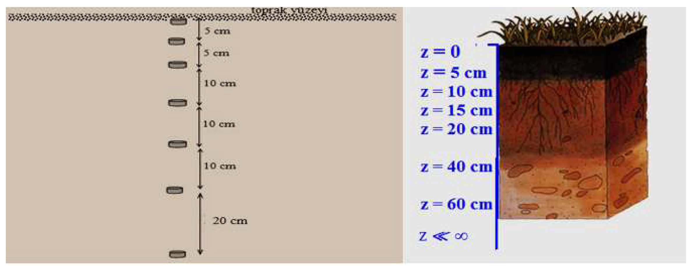
Figure 2.
a. The average soil temperature data during 01/12/2019- 30/11/2020 at non-alkaline soil (0C). b. The average soil temperature data during 01/12/2019- 30/11/2020 at alkaline soil (0C).
Figure 2.
a. The average soil temperature data during 01/12/2019- 30/11/2020 at non-alkaline soil (0C). b. The average soil temperature data during 01/12/2019- 30/11/2020 at alkaline soil (0C).
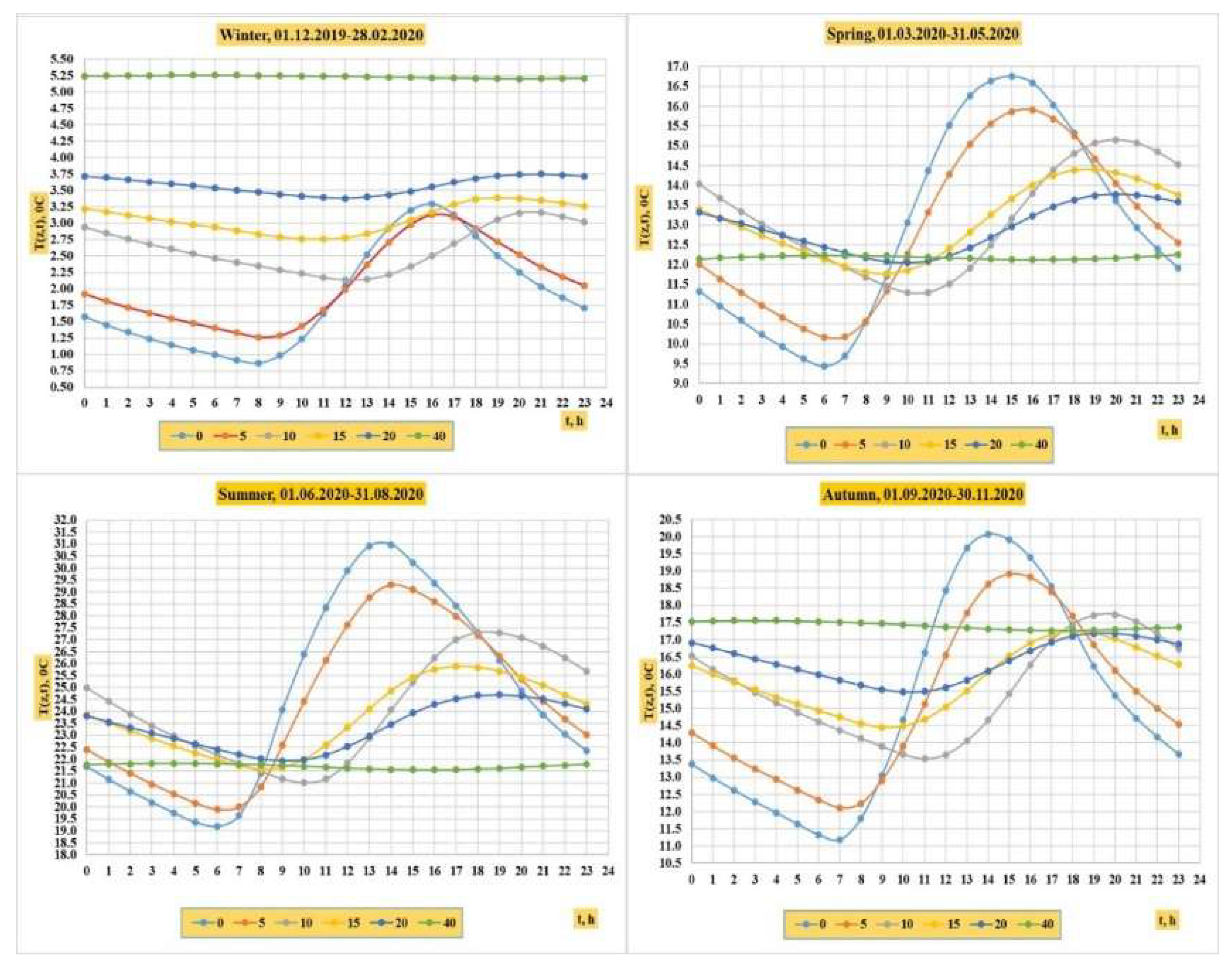
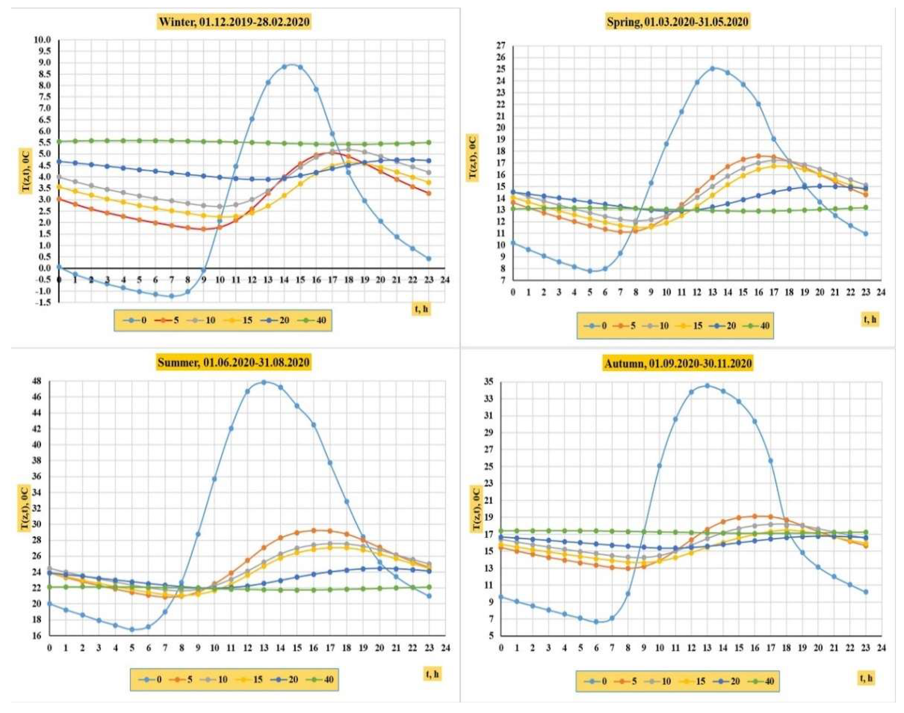
Figure 5.
Heat flux (W m-2) from the soil surface calculating according to proposed method (M8) at non- alkaline and alkaline soil.
Figure 5.
Heat flux (W m-2) from the soil surface calculating according to proposed method (M8) at non- alkaline and alkaline soil.
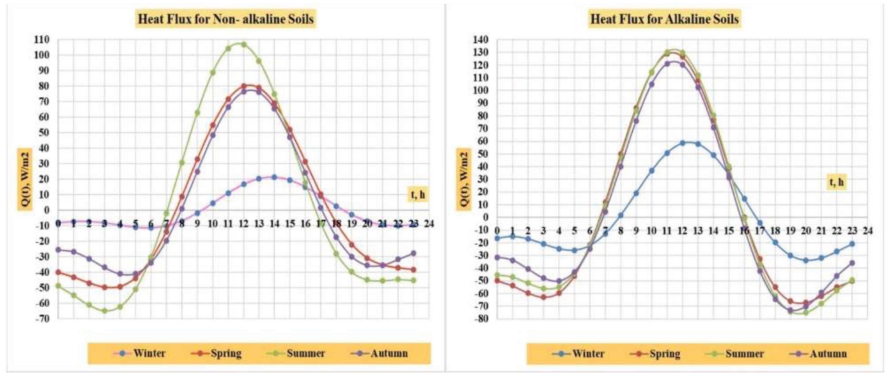

Table 1.
Some physical and chemical soil properties.
| Soil | Depth | Texture | ρb | θ | OM | pH | EC | ESP |
|---|---|---|---|---|---|---|---|---|
| cm | kg m-3 | m3 m-3 | % | 01:01 | dS m-1 | % | ||
| Non alkaline |
0-10 | CL | 974.3 | 0.1449 | 1.40 | 8.42 | 0.3877 | 3.2 |
| 10-20 | CL | 1023.3 | 0.1521 | 1.62 | 8.26 | 0.4126 | 3.4 | |
| 20-25 | L | 1105.4 | 0.1717 | 2.35 | 8.01 | 0.5417 | 3.1 | |
| 25-30 | SCL | 1245.7 | 0.1806 | 2.81 | 8.03 | 0.5524 | 3.5 | |
| 30-35 | SL | 1158.1 | 0.1907 | 3.07 | 8.05 | 0.5507 | 3.7 | |
| 35-40 | SL | 1216.5 | 0.1925 | 2.66 | 8.12 | 0.5121 | 3.6 | |
| 0-40 | 1120.6 | 0.1721 | 2.32 | 8.15 | 0.4929 | 3.4 | ||
| Alkaline | 0-10 | CL | 1072,7 | 0,1463 | 1,26 | 8,70 | 1,2724 | 17,9 |
| 10-20 | CL | 1125,6 | 0,1628 | 1,24 | 8,56 | 1,2320 | 17,6 | |
| 20-25 | L | 1194,0 | 0,1738 | 0,91 | 8,54 | 0,9842 | 18,2 | |
| 25-30 | SCL | 1247,8 | 0,1874 | 1,12 | 9,45 | 0,8252 | 17,9 | |
| 30-35 | SL | 1160,4 | 0,1945 | 1,08 | 9,50 | 0,6945 | 17,5 | |
| 35-40 | SL | 1218,0 | 0,1948 | 1,55 | 9,68 | 0,5429 | 17,6 | |
| 0-40 | 1169,7 | 0,1766 | 1,19 | 9,07 | 0,9252 | 17,8 |
CL: clay loam; L: loam; SCl: sandy clay loam; S: sandy loam; ρb: soil bulk density; θ: volumetric water content OM: soil organic matter; pH: soil pH; EC: soil electrical conductivity; ESP: exchangeable sodium percentage.
Table 2.
Parameters of the nonalkaline soils surfaces and model performance for all seasons.
| The number of harmonics in the equation (2.9) | |||||||||
|---|---|---|---|---|---|---|---|---|---|
| m = 1 | m = 2 | ||||||||
| Winter | Spring | Summer | Autumn | Winter | Spring | Summer | Autumn | ||
| n* | 24 | 24 | 24 | 24 | n | 24 | 24 | 24 | 24 |
| p | 3 | 3 | 3 | 3 | p | 5 | 5 | 5 | 5 |
| df | 21 | 21 | 21 | 21 | df | 19 | 19 | 19 | 19 |
| To | 1.8643 | 12.9127 | 24.5478 | 15.0455 | To | 1.8643 | 12.9127 | 24.5478 | 15.0455 |
| Ta1 | 1.0327 | 3.4375 | 5.4270 | 3.9363 | Ta1 | 0.3598 | 0.7946 | 1.5067 | 1.3964 |
| ε1 | 1.8468 | 2.1760 | 2.3607 | 2.2011 | ε1 | 4.5802 | -0.8483 | -0.4932 | -0.9846 |
| Statistical parameters of approximation | |||||||||
| R2 | 0.8862 | 0.9475 | 0.9227 | 0.8845 | R2 | 0.9938 | 0.9981 | 0.9938 | 0.9958 |
| R2adj | 0.8810 | 0.9451 | 0.9192 | 0.8792 | R2adj | 0.9935 | 0.9980 | 0.9935 | 0.9956 |
| D | 0.9951 | 0.9991 | 0.9990 | 0.9979 | D | 0.9984 | 0.9995 | 0.9984 | 0.9989 |
| UI | 0.0466 | 0.0362 | 0.0405 | 0.0560 | UI | 0.0152 | 0.0041 | 0.0063 | 0.0063 |
| RMSE | 0.28 | 0.61 | 1.19 | 1.08 | RMSE | 0.07 | 0.12 | 0.35 | 0.22 |
| AICc | -1.48 | 0.08 | 1.41 | 1.21 | AICc | -2.25 | -1.11 | 1.02 | 0.04 |
*n – number of observations, p – number of parameters, df – degree of freedom,.
Table 3.
Parameters of the alkaline soils surfaces and model performance for all seasons.
| The number of harmonics in the equation (2.9) | |||||||||
|---|---|---|---|---|---|---|---|---|---|
| m = 1 | m = 2 | ||||||||
| Winter | Spring | Summer | Autumn | Winter | Spring | Summer | Autumn | ||
| n* | 24 | 24 | 24 | 24 | n | 24 | 24 | 24 | 24 |
| p | 3 | 3 | 3 | 3 | p | 5 | 5 | 5 | 5 |
| df | 21 | 21 | 21 | 21 | df | 19 | 19 | 19 | 19 |
| To | 2,4052 | 14,8979 | 28,9658 | 17,3838 | To | 2,4052 | 14,8979 | 28,9658 | 17,3838 |
| Ta1 | 4,4773 | 7,9065 | 14,6342 | 13,1626 | Ta2 | 1,8615 | 2,5074 | 4,9455 | 5,3725 |
| ε1 | 2,3250 | 2,5422 | 2,5776 | 2,6118 | ε2 | -1,0822 | -0,4765 | -0,5980 | -0,6023 |
| Statistical parameters of approximation | |||||||||
| R2 | 0,8424 | 0,9068 | 0,8943 | 0,8428 | R2 | 0,9880 | 0,9980 | 0,9965 | 0,9846 |
| R2adj | 0,8352 | 0,9026 | 0,8895 | 0,8356 | R2adj | 0,9874 | 0,9979 | 0,9963 | 0,9839 |
| D | 0,9525 | 0,9938 | 0,9934 | 0,9801 | D | 0,9970 | 0,9995 | 0,9991 | 0,9961 |
| UI | 0,1922 | 0,0966 | 0,1068 | 0,1785 | UI | 0,0451 | 0,0081 | 0,0105 | 0,0311 |
| RMSE | 1,46 | 1,92 | 3,80 | 4,22 | RMSE | 0,43 | 0,29 | 0,73 | 1,39 |
| AICc | 1,83 | 2,37 | 3,74 | 3,95 | AICc | 1,39 | 0,64 | 2,47 | 3,76 |
Table 5.
Thermal properties of nonalkaline soils.
| Models | Harmoni | Season | 10-6 κ | λ | d | e | V·10-5 | Λ | Cv |
|---|---|---|---|---|---|---|---|---|---|
| m2s-1 | Wm-1 oC-1 | cm | Ws0.5m-2 oC-1 | m s-1 | m | kJ m-3 oC-1 | |||
| Layered methods with boundary conditions: ∂T(∞.t)/∂z =0 | |||||||||
| M1 | m=1 | Winter | 0.5376 | 1.0099 | 12.16 | 1377.35 | 0.8843 | 0.76 | 1878.49 |
| Spring | 0.6972 | 1.4824 | 13.85 | 1775.39 | 1.0070 | 0.87 | 2126.30 | ||
| Summer | 0.7422 | 1.1846 | 14.29 | 1375.01 | 1.0390 | 0.90 | 1596.04 | ||
| Autumn | 0.6066 | 1.0591 | 12.92 | 1359.94 | 0.9393 | 0.81 | 1746.15 | ||
| M2 | m=2 | Winter | 1.3235 | 2.4861 | 19.08 | 2161.05 | 1.3874 | 1.20 | 1878.49 |
| Spring | 0.8752 | 1.8610 | 15.51 | 1989.24 | 1.1283 | 0.98 | 2126.30 | ||
| Summer | 0.9287 | 1.4823 | 15.98 | 1538.12 | 1.1622 | 1.00 | 1596.04 | ||
| Autumn | 0.8807 | 1.5378 | 15.56 | 1638.65 | 1.1318 | 0.98 | 1746.15 | ||
| M3 | m=2 | Winter | 0.7050 | 1.3243 | 13.92 | 1577.22 | 1.0126 | 0.87 | 1878.49 |
| Spring | 0.7202 | 1.5313 | 14.07 | 1804.43 | 1.0234 | 0.89 | 2126.30 | ||
| Summer | 0.7643 | 1.2199 | 14.50 | 1395.33 | 1.0543 | 0.91 | 1596.04 | ||
| Autumn | 0.6693 | 1.1688 | 13.57 | 1428.57 | 0.9867 | 0.85 | 1746.15 | ||
| M4 | m=1 | Winter | 1.0292 | 1.9334 | 16.82 | 1905.73 | 1.2235 | 1.06 | 1878.49 |
| Spring | 0.7969 | 1.6945 | 14.80 | 1898.17 | 1.0766 | 0.93 | 2126.30 | ||
| Summer | 0.8174 | 1.3046 | 14.99 | 1442.97 | 1.0903 | 0.94 | 1596.04 | ||
| Autumn | 0.6211 | 1.0845 | 13.07 | 1376.13 | 0.9504 | 0.82 | 1746.15 | ||
| Point methodsmethods with boundary conditions: ∂T(∞.t)/∂z =0 | |||||||||
| M5 | m=1 | Winter | 0.7550 | 1.4183 | 14.41 | 1632.27 | 1.0479 | 0.91 | 1878.49 |
| Spring | 0.8756 | 1.8618 | 15.52 | 1989.67 | 1.1285 | 0.98 | 2126.30 | ||
| Summer | 0.9325 | 1.4882 | 16.01 | 1541.20 | 1.1646 | 1.01 | 1596.04 | ||
| Autumn | 0.6821 | 1.1911 | 13.70 | 1442.14 | 0.9960 | 0.86 | 1746.15 | ||
| Winter | 0.7164 | 1.3458 | 14.04 | 1590.02 | 1.0208 | 0.88 | 1878.49 | ||
| Μ6 | m=2 | Spring | 0.8843 | 1.8802 | 15.59 | 1999.48 | 1.1341 | 0.98 | 2126.30 |
| Summer | 1.0022 | 1.5996 | 16.60 | 1597.80 | 1.2073 | 1.04 | 1596.04 | ||
| Autumn | 0.7614 | 1.3295 | 14.47 | 1523.63 | 1.0523 | 0.91 | 1746.15 | ||
| Point methodsmethods with boundary conditions: ∂T(L. t)/∂z=0 | |||||||||
| Μ7 | m=1 | Winter | 0.8008 | 1.5042 | 14.84 | 1680.97 | 1.0792 | 0.93 | 1878.49 |
| Spring | 0.9584 | 2.0379 | 16.24 | 2081.65 | 1.1807 | 1.02 | 2126.30 | ||
| Summer | 1.0237 | 1.6339 | 16.78 | 1614.84 | 1.2202 | 1.05 | 1596.04 | ||
| Autumn | 0.6766 | 1.1815 | 13.64 | 1436.31 | 0.9920 | 0.86 | 1746.15 | ||
| Μ8 | m=2 | Winter | 0.7533 | 1.4151 | 14.39 | 1630.40 | 1.0467 | 0.90 | 1878.49 |
| Spring | 0.9725 | 2.0678 | 16.35 | 2096.83 | 1.1893 | 1.03 | 2126.30 | ||
| Summer | 1.1035 | 1.7613 | 17.42 | 1676.63 | 1.2669 | 1.09 | 1596.04 | ||
| Autumn | 0.7854 | 1.3714 | 14.70 | 1547.45 | 1.0688 | 0.92 | 1746.15 | ||
* M1 –Amplitude, M2 –Arctangent, M3 – Logarithm, M4 – Phase, M5–M8 – Improved methods.
Table 6.
Thermal properties of alkaline soils.
| Models | Harmoni | Season | 10-6 κ | λ | d | e | V·10-5 | Λ | Cv |
|---|---|---|---|---|---|---|---|---|---|
| m2s-1 | Wm-1 oC-1 | cm | Ws0.5m-2 oC-1 | m s-1 | m | kJ m-3 oC-1 | |||
| Layered methods with boundary conditions: ∂T(∞.t)/∂z =0 | |||||||||
| M1 | m=1 | Winter | 7.2882 | 14.6792 | 44.77 | 5437.41 | 3.2558 | 2.8130 | 2014.11 |
| Spring | 92.7680 | 217.9169 | 159.73 | 22625.17 | 3.2558 | 10.0360 | 2349.05 | ||
| Summer | 209.4553 | 342.9403 | 240.01 | 23695.88 | 17.4540 | 15.0802 | 1637.30 | ||
| Autumn | 35.4889 | 65.5351 | 98.79 | 11000.88 | 7.1845 | 6.2074 | 1846.64 | ||
| M2 | m=2 | Winter | 3.6121 | 7.2751 | 31.52 | 3827.91 | 2.2921 | 1.9803 | 2014.11 |
| Spring | 7.2158 | 16.9502 | 44.55 | 6310.06 | 2.2921 | 2.7990 | 2349.05 | ||
| Summer | 349.4319 | 572.1234 | 310.00 | 30606.13 | 22.5439 | 19.4779 | 1637.30 | ||
| Autumn | 3.4077 | 6.2928 | 30.61 | 3408.88 | 2.2263 | 1.9235 | 1846.64 | ||
| M3 | m=2 | Winter | 6.7248 | 13.5445 | 43.01 | 5223.03 | 3.1274 | 2.7021 | 2014.11 |
| Spring | 24.9110 | 58.5173 | 82.77 | 11724.34 | 3.1274 | 5.2006 | 2349.05 | ||
| Summer | 143.4528 | 234.8747 | 198.63 | 19610.19 | 14.4445 | 12.4801 | 1637.30 | ||
| Autumn | 9.9721 | 18.4148 | 52.37 | 5831.42 | 3.8084 | 3.2904 | 1846.64 | ||
| M4 | m=1 | Winter | 1.8315 | 3.6888 | 22.44 | 2725.74 | 1.6321 | 1.4101 | 2014.11 |
| Spring | 7.0423 | 16.5427 | 44.01 | 6233.75 | 1.6321 | 2.7651 | 2349.05 | ||
| Summer | 1399.3616 | 2291.1688 | 620.36 | 61248.03 | 45.1142 | 38.9786 | 1637.30 | ||
| Autumn | 1.7919 | 3.3090 | 22.20 | 2471.93 | 1.6144 | 1.3948 | 1846.64 | ||
| Point methodsmethods with boundary conditions: ∂T(∞.t)/∂z =0 | |||||||||
| M5 | m=1 | Winter | 0.2669 | 0.5376 | 8,57 | 1040.56 | 0.6231 | 0.5383 | 2014.11 |
| Spring | 0.3423 | 0.8041 | 9.70 | 1374.399 | 0.6231 | 0.6097 | 2349.05 | ||
| Summer | 0.2085 | 0.3414 | 7.57 | 747.62 | 0.5507 | 0.4758 | 1637.30 | ||
| Autumn | 0.1557 | 0.2876 | 6.54 | 728.77 | 0.4759 | 0.4112 | 1846.64 | ||
| Winter | 0.2572 | 0.5181 | 8.41 | 1021.49 | 0.6116 | 0.5285 | 2014.11 | ||
| Μ6 | m=2 | Spring | 0.3364 | 0.7903 | 9.62 | 1362.489 | 0.6116 | 0.6044 | 2349.05 |
| Summer | 0.2106 | 0.3448 | 7.61 | 751.36 | 0.5534 | 0.4782 | 1637.30 | ||
| Autumn | 0.1587 | 0.2931 | 6.61 | 735.75 | 0.4805 | 0.4152 | 1846.64 | ||
| Point methodsmethods with boundary conditions: ∂T(L. t)/∂z=0 | |||||||||
| Μ7 | m=1 | Winter | 0.2477 | 0.4988 | 8.25 | 1002.33 | 0.6002 | 0.5185 | 2014.11 |
| Spring | 0.3261 | 0.7661 | 9.47 | 1341.49 | 0.6887 | 0.5951 | 2349.05 | ||
| Summer | 0.1912 | 0.3130 | 7.25 | 715.85 | 0.5273 | 0.4556 | 1637.30 | ||
| Autumn | 0.1409 | 0.2601 | 6.22 | 693.09 | 0.4526 | 0.3911 | 1846.64 | ||
| Μ8 | m=2 | Winter | 0.2371 | 0.4775 | 8.07 | 980.67 | 0.5872 | 0.5073 | 2014.11 |
| Spring | 0.3214 | 0.7549 | 9.40 | 1331.69 | 0.6837 | 0.5907 | 2349.05 | ||
| Summer | 0.1935 | 0.3168 | 7.29 | 720.16 | 0.5305 | 0.4583 | 1637.30 | ||
| Autumn | 0.1431 | 0.2643 | 6.27 | 698.66 | 0.4563 | 0.3942 | 1846.64 | ||
Table 7.
Effectiveness of models (M1–M8) for predicting the temperature of non-alkaline soil at four depths z = 5, 10, and 15 cm during the year (from 01.12.2019 to 20.11.2020) for four seasons
Table 7.
Effectiveness of models (M1–M8) for predicting the temperature of non-alkaline soil at four depths z = 5, 10, and 15 cm during the year (from 01.12.2019 to 20.11.2020) for four seasons
| Depth | M1 | M2 | M3 | M4 | M5 | M6 | M7 | M8 | |
|---|---|---|---|---|---|---|---|---|---|
| z. m | Winter | ||||||||
| r | 0.05 | 0.9232 | 0.9445 | 0.9330 | 0.9385 | 0.9349 | 0.9711 | 0.9372 | 0.9838 |
| 0.10 | 0.8052 | 0.6155 | 0.7462 | 0.6990 | 0.7313 | 0.6292 | 0.7120 | 0.7096 | |
| 0.15 | 0.9581 | 0.9236 | 0.9679 | 0.9604 | 0.9668 | 0.8538 | 0.9646 | 0.9968 | |
| RMSE | 0.05 | 0.3360 | 0.3003 | 0.3200 | 0.3106 | 0.3168 | 0.2631 | 0.3136 | 0.2494 |
| 0.10 | 0.8321 | 0.8845 | 0.8450 | 0.8575 | 0.8487 | 0.8840 | 0.8523 | 0.8537 | |
| 0.15 | 1.2914 | 1.3009 | 1.2918 | 1.2937 | 1.2923 | 1.3087 | 1.2923 | 1.2907 | |
| z. m | Spring | ||||||||
| r | 0.05 | 0.9688 | 0.9735 | 0.9696 | 0.9718 | 0.9735 | 0.9880 | 0.9754 | 0.9956 |
| 0.10 | 0.7836 | 0.7355 | 0.7767 | 0.7552 | 0.7354 | 0.6672 | 0.7124 | 0.6944 | |
| 0.15 | 0.9855 | 0.9853 | 0.9863 | 0.9870 | 0.9853 | 0.9194 | 0.9829 | 0.9926 | |
| RMSE | 0.05 | 0.5680 | 0.5078 | 0.5584 | 0.5306 | 0.5077 | 0.3395 | 0.4885 | 0.2488 |
| 0.10 | 0.9277 | 1.0431 | 0.9436 | 0.9946 | 1.0433 | 1.2158 | 1.0874 | 1.1292 | |
| 0.15 | 0.2607 | 0.2529 | 0.2539 | 0.2445 | 0.2529 | 0.5037 | 0.2613 | 0.2257 | |
| z. m | Summer | ||||||||
| r | 0.05 | 0.9562 | 0.9608 | 0.9569 | 0.9584 | 0.9609 | 0.9867 | 0.9628 | 0.9944 |
| 0.10 | 0.8022 | 0.7591 | 0.7965 | 0.7836 | 0.7583 | 0.6704 | 0.7384 | 0.7097 | |
| 0.15 | 0.9731 | 0.9797 | 0.9747 | 0.9775 | 0.9797 | 0.9169 | 0.9794 | 0.9968 | |
| RMSE | 0.05 | 1.0992 | 1.0228 | 1.0879 | 1.0636 | 1.0216 | 0.6347 | 0.9981 | 0.5228 |
| 0.10 | 1.4630 | 1.6310 | 1.4840 | 1.5334 | 1.6341 | 2.0207 | 1.6962 | 1.8133 | |
| 0.15 | 0.9299 | 0.9086 | 0.9237 | 0.9133 | 0.9088 | 1.2002 | 0.9086 | 0.8647 | |
| z. m | Autumn | ||||||||
| r | 0.05 | 0.9411 | 0.9475 | 0.9433 | 0.9416 | 0.9437 | 0.9832 | 0.9439 | 0.9952 |
| 0.10 | 0.7739 | 0.6914 | 0.7519 | 0.7686 | 0.7477 | 0.6151 | 0.7430 | 0.6949 | |
| 0.15 | 0.9626 | 0.9647 | 0.9670 | 0.9640 | 0.9675 | 0.8578 | 0.9678 | 0.9982 | |
| RMSE | 0.05 | 0.8609 | 0.7911 | 0.8378 | 0.8550 | 0.8337 | 0.4593 | 0.8329 | 0.3279 |
| 0.10 | 1.1172 | 1.3245 | 1.1691 | 1.1294 | 1.1794 | 1.5869 | 1.1842 | 1.3093 | |
| 0.15 | 0.8934 | 0.9085 | 0.8888 | 0.8918 | 0.8886 | 1.1820 | 0.8876 | 0.8570 | |
Table 8.
Effectiveness of models (M1–M8) for predicting the temperature of alkaline soil at four depths z = 5, 10, and 15 cm during the year (from 01.12.2019 to 20.11.2020) for four seasons.
Table 8.
Effectiveness of models (M1–M8) for predicting the temperature of alkaline soil at four depths z = 5, 10, and 15 cm during the year (from 01.12.2019 to 20.11.2020) for four seasons.
| Depth | M1 | M2 | M3 | M4 | M5 | M6 | M7 | M8 | |
|---|---|---|---|---|---|---|---|---|---|
| z. m | Winter | ||||||||
| r | 0.05 | 0.7185 | 0.7470 | 0.7214 | 0.7832 | 0.9235 | 0.9068 | 0.9284 | 0.9726 |
| 0.10 | 0.5886 | 0.6567 | 0.5954 | 0.7403 | 0.9560 | 0.7924 | 0.9535 | 0.9912 | |
| 0.15 | 0.5883 | 0.6882 | 0.5986 | 0.8022 | 0.8346 | 0.5227 | 0.8020 | 0.8067 | |
| RMSE | 0.05 | 2.4549 | 2.2906 | 2.4384 | 2.0803 | 1.2065 | 1.5692 | 1.1705 | 1.1284 |
| 0.10 | 2.7519 | 2.5047 | 2.7263 | 2.2188 | 1.5476 | 1.9136 | 1.5437 | 1.5220 | |
| 0.15 | 2.2593 | 1.9043 | 2.2218 | 1.5191 | 1.0836 | 1.6181 | 1.1023 | 1.1018 | |
| z. m | Spring | ||||||||
| r | 0.05 | 0.6835 | 0.7376 | 0.7035 | 0.7385 | 0.9293 | 0.9132 | 0.9331 | 0.9540 |
| 0.10 | 0.5196 | 0.6465 | 0.5670 | 0.6486 | 0.9783 | 0.8614 | 0.9791 | 0.9994 | |
| 0.15 | 0.5014 | 0.6888 | 0.5728 | 0.6916 | 0.8939 | 0.6396 | 0.8801 | 0.8914 | |
| RMSE | 0.05 | 4.5860 | 4.0131 | 4.3748 | 4.0038 | 1.7992 | 2.2409 | 1.7480 | 1.7239 |
| 0.10 | 4.9233 | 3.8579 | 4.5224 | 3.8411 | 0.6147 | 1.5951 | 0.5871 | 0.4455 | |
| 0.15 | 4.8718 | 3.3972 | 4.3017 | 3.3750 | 1.3436 | 2.0376 | 1.3819 | 1.3620 | |
| z. m | Summer | ||||||||
| r | 0.05 | 0.6795 | 0.6762 | 0.6825 | 0.6705 | 0.9621 | 0.9254 | 0.9662 | 0.9903 |
| 0.10 | 0.5048 | 0.4969 | 0.5121 | 0.4832 | 0.9491 | 0.7310 | 0.9332 | 0.9510 | |
| 0.15 | 0.5192 | 0.5074 | 0.5300 | 0.4870 | 0.6040 | 0.2673 | 0.5335 | 0.5400 | |
| RMSE | 0.05 | 10.0685 | 10.1238 | 10.0178 | 10.2194 | 5.3090 | 6.1000 | 5.2119 | 5.2323 |
| 0.10 | 10.7883 | 10.8938 | 10.6919 | 11.0775 | 4.8664 | 5.8961 | 4.8587 | 4.8479 | |
| 0.15 | 10.8287 | 10.9800 | 10.6913 | 11.2458 | 5.6042 | 6.6876 | 5.6402 | 5.6379 | |
| z. m | Autumn | ||||||||
| r | 0.05 | 0.6486 | 0.7235 | 0.6794 | 0.7608 | 0.9502 | 0.9051 | 0.9537 | 0.9954 |
| 0.10 | 0.4343 | 0.6165 | 0.5100 | 0.7038 | 0.9178 | 0.6053 | 0.8909 | 0.9116 | |
| 0.15 | 0.3836 | 0.6590 | 0.5003 | 0.7802 | 0.5476 | 0.1492 | 0.4487 | 0.4559 | |
| RMSE | 0.05 | 8.3498 | 7.1940 | 7.8738 | 6.6146 | 3.0722 | 4.5734 | 2.9157 | 2.9487 |
| 0.10 | 8.5686 | 6.5279 | 7.7026 | 5.5862 | 1.6225 | 4.1208 | 1.5893 | 1.5858 | |
| 0.15 | 8.3795 | 5.6865 | 7.1937 | 4.5811 | 2.3271 | 4.6643 | 2.3667 | 2.3666 | |
Disclaimer/Publisher’s Note: The statements, opinions and data contained in all publications are solely those of the individual author(s) and contributor(s) and not of MDPI and/or the editor(s). MDPI and/or the editor(s) disclaim responsibility for any injury to people or property resulting from any ideas, methods, instructions or products referred to in the content. |
© 2025 by the authors. Licensee MDPI, Basel, Switzerland. This article is an open access article distributed under the terms and conditions of the Creative Commons Attribution (CC BY) license (http://creativecommons.org/licenses/by/4.0/).
Copyright: This open access article is published under a Creative Commons CC BY 4.0 license, which permit the free download, distribution, and reuse, provided that the author and preprint are cited in any reuse.


