Submitted:
25 August 2025
Posted:
26 August 2025
You are already at the latest version
Abstract
Sub-sea environments host rich biodiversity and resources, playing a crucial role in climate regulation while supporting human activities such as fishing, transport, and resource extraction. To maintain healthy underwater ecosystems and ensure sustainable operations, accurate mapping and monitoring are essential. Among available technologies, airborne LiDAR bathymetry (ALB) stands out for its ability to capture detailed subsea data, but handling the enormous datasets it generates remains a major challenge. In this study, we propose a novel preprocessing pipeline combined with deep learning models—Long Short-Term Memory (LSTM) and Bidirectional LSTM (BiLSTM)—to classify submerged environments using data from Fjøløy, Stavanger, Norway. LSTM achieved a higher classification accuracy (95.22%) compared to BiLSTM (94.85%). To further assess robustness, classification reliability was evaluated through confidence scores, offering insights into model dependability. The results demonstrate the potential of deep learning for ALB classification and provide practical value for mapping authorities and practitioners in producing reliable seabed maps and nautical charts.
Keywords:
airborne LiDAR bathymetry
; deep learning
; LSTM
; BiLSTM
; underwater
; classification
; seabed
; vegetation
; submerged environments
1. Introduction
Our planet is 71% covered by water, representing nearly three-quarters of the Earth’s surface [1]. These water bodies are essential for life, producing approximately 50% of the oxygen required by living organisms, absorbing 25% of global CO2 emissions and a significant portion of the heat associated with these emissions [2]. They play a vital role in the planet’s sustainable development [3]. At the same time, many human activities depend on oceans and seas, including resource extraction, fishing, and the transportation of goods and people [4]. However, these activities also impact the underwater ecosystem. Therefore, monitoring subsea environments is crucial in assessing the health of the underwater ecosystem while ensuring these operations remain sustainable. This can be achieved through accurate mapping of underwater landscapes [5].
In Norway, marine resources are the backbone of the nation’s economy. The oil and gas industry contributes 14% of the national GDP and 39% of export revenue, while the seafood sector accounts for 1.6% of GDP and 11% of exports [6]. Accurate mapping of Norway’s subsea environments is fundamental for maintaining economic stability and protecting the marine ecosystem. The Norwegian Mapping Authority (NMA)1 is responsible for these mapping efforts using advanced technologies and data-driven tools to provide reliable geospatial information [7].
In recent years, technological advancements have shown significant potential in the mapping of subsea environments, employing technologies such as Multi-Beam Echo Sounders (MBES) [8], satellite remote sensing [9], and Light Detection and Ranging (LiDAR) [10]. Among these, airborne LiDAR Bathymetry (ALB) stands out as one of the most promising techniques, capable of scanning submerged surfaces with high precision [11,12]. However, despite its potential, bathymetric LiDAR presents significant challenges. The technology generates massive volumes of data that demand extensive human intervention for processing. This makes the study of ALB data both time and resource-intensive, limiting its scalability and deployment in real-world applications [12,13,14].
Deep learning (DL) offers a transformative solution to address these challenges by enabling the analysis and classification of complex ALB data. At the core of DL, neural networks excel at identifying intricate patterns in marine ecosystems, achieving higher accuracy and reliability in subsea classification compared to traditional methods [15,16]. Despite this promising potential, previous studies by the authors [17] highlight that the application of DL for classifying ALB data remains unexplored compared to other research domains. This presents an opportunity to leverage DL’s capabilities to address the limitations of traditional techniques and advance underwater mapping efforts. Furthermore, DL can handle sequential data by focusing on specific methods that help models understand and retain important information over time. It can be retrieved using DL models such as the Long Short-Term Memory (LSTM) and Bidirectional Long Short-Term Memory (BiLSTM) network. These are popular deep-learning models for handling sequential data because they are designed to remember information over longer periods. LSTM models understand sequences with greater precision, balancing between remembering important details and focusing on what matters most in each step of the sequence [18].
Interestingly, despite the popularity of these models, to the authors’ knowledge, these DL models have yet to be deployed in combination with ALB data. The combined use of these DL models may provide potential benefits for the mapping authorities handling such big data. Importantly, this study also explores the reliability of classifying specific points in bathymetric LiDAR data, which plays a crucial role in ensuring accurate subsea mapping for seabed and vegetation. This reliability aspect is vital for enhancing safe navigability in maritime transportation and ensuring precise resource management in underwater environments. Hence, the objective of this work is to improve the ALB data classification of underwater environments through the application of two deep learning models: LSTM and BiLSTM. To achieve this, the following research questions will be answered:
- RQ1: Which deep learning model between LSTM and BiLSTM performs better in classifying subsea environments?
- RQ2: How reliable is the classification of a specific point in bathymetric LiDAR data for seabed and vegetation mapping?
A novel preprocessing technique is introduced to handle large-scale bathymetric LiDAR data, offering a reliable method for labeling and extracting meaningful information, thereby enhancing data analysis workflows. The deployment of advanced deep learning models, LSTM and BiLSTM, on bathymetric LiDAR data retrieved from a Norwegian test area ensures accurate classification into key categories, such as sea surface, vegetation, seabed, water, and noise. With this work, the authors aim to provide insights for researchers and practitioners dealing with bathymetric LiDAR data. The potential implications of this work for seabed mapping and maritime navigation are further elaborated in the discussion section.
2. Related Work
The authors of this research conducted a systematic literature review to examine previous scientific studies on the application of DL to bathymetric LiDAR data. The findings of this review are presented in [17]. This section highlights the key insights from these studies, as summarized in Table 1. The studies listed in the table have been adapted from [17].
In [19], the authors utilized data retrieved from the artificial reef Rosenort in the Baltic Sea to demonstrate the use of a multilayer perceptron (MLP) neural network with softmax activation for seabed object detection and classification. The network training incorporated both point cloud geometry properties and the full waveform. The results achieved nearly 100% accuracy in classifying the seabed and water surface, while seabed object location classification exceeded 80% accuracy. These findings significantly improved object detection performance compared to other well-known classification techniques. For data preprocessing, the authors applied Gaussian decomposition to the full waveform. The pre-processed dataset comprised 6198 vectors, with 80% used for training and 20% reserved for validation during the error back-propagation algorithm process.
In [20], the researchers modeled the seabed using data retrieved from the same location as [19]. Their study addressed the issue of data imbalance among three categories namely: water surface, bottom, and bottom objects. To mitigate this asymmetry, they proposed to use 53 Synthetic Minority Oversampling Technique (SMOTE) algorithms for generating synthetic data to balance the dataset. For classification, they employed a Multi-Layer Perceptron (MLP) neural network to process the point cloud data. Initially, to compare the result with the balanced data, first, they obtained the accuracy for the unbalanced data and data with downsampling which is 89.6% and 93.5%, respectively. With the balanced data, the accuracy achieved varied from 95.8% to 97.0%, depending on the oversampling algorithm used.
In [21], the authors highlighted the limitations of PointNet and its successor PointNet++ in handling a large-scale spatial scene with millions of possible points, despite their popularity in point cloud segmentation. When segmenting coastal zones, accurately identifying the small number of points at the interface between the seabed and the water surface is crucial. To address this challenge, the study introduced a voxel sampling pre-processing (VSP) approach for semantic segmentation of a large-scale airborne Lidar bathymetry (ALB) point cloud. The dataset, collected from coastal-urban scenes of Tampa Bay, Florida, USA, was segmented into two classes: water surface and seabed. The authors applied an adaptive sampling strategy, sampling sparse data at a higher rate and dense data at a lower rate to account for sensor characteristics. The LiDAR system’s broom laser pattern produces denser data in the center and sparser data at the edges, necessitating this differentiated approach. Additionally, they incorporated the superpoint graph (SPG) algorithm, a superpixel-based method for 3D point clouds, to create a downsampled version of the original dataset. By combining the VSP approach with SPG, the validation accuracy reached 72.45%.
In [22], the authors introduced a deep-learning model for classifying airborne LiDAR bathymetry (ALB) data, with applications in the ocean–land discrimination and waterline extraction. The study was conducted at a test location of Qinshan Island of Lianyungang City, Jiangsu Province, China. Their proposed approach named multichannel voting convolutional neural network (MVCNN), leveraged multichannel green laser waveforms. By utilizing both deep and shallow LiDAR channels, they collected multiple green laser waveforms, which were then fed into a multichannel input module. Each green channel waveform was processed using a one-dimensional (1-D) Convolutional Neural Network (CNN). To enhance classification performance, they introduced a multichannel voting module, which applied majority voting on the predicted categories from each 1-D CNN model. This approach achieved an accuracy of 99.41%. Further analysis indicated that increasing the number of laser channels could further improve classification accuracy.
In [9], the authors proposed a deep learning framework based on a 2D CNN for nearshore bathymetric inversion at three particular locations in the United States: Appalachian Bay (AB), Virgin Islands (VI), and Cat Island (CI). Their approach used ICESat-2 LiDAR and Sentinel-2 Imagery datasets. The framework, named “DL-NB”, leveraged the full use of the initial multi-spectral information from Sentinel-2, incorporating both each bathymetric point and its adjacent area during training. A critical aspect of the study involved accurately determining the sea level and seafloor. This was achieved using histogram statistics at each segment near the sea level, guided by two key rules: the point density near the sea level is higher closer to the surface, and the sea level is always positioned above the seafloor. The RMSE of the DL-NB varied across locations, achieving 1.01 m in AB, 1.80 m in VI, and 0.28 m in CI. To assess the portability of the DL-NB framework, the authors conducted cross-validation between different study areas where the model performed poorly, which can be concluded that the diversity of environmental factors may limit the portability.
In [23], the authors conducted a classification study using bathymetric data from the Baltic Sea location as [19,20], approximately 25 km north of the city of Rostock. The classification was divided into two parts, one was the classification of the entire point cloud, and another was the classification of the points excluding the points belonging to the water surface. Both classifications were performed using a Random Forest (RF) classifier, despite challenges such as low transparency of the water, low salinity, and small waves. To extract full waveform-based features, they applied the Gaussian function, considering parameters such as amplitude, echo width, number of the next echo, quantity of return for a single impulse, and normalized number of echoes, obtained by dividing the echo number by the total number of echoes in the full waveform of a current point. The RF model was trained with a total of 6,198 points for the full dataset and 3,469 points after excluding water surface points. The coefficient of determination (R2) was used as a key performance metric, comparing predicted and observed class values. The model achieved coefficient of determination was 0.99 for the full dataset, while the second dataset’s coefficient was 0.92. The classification accuracy was 100% for the water surface, 99.9% for the seabed, and 60% for objects. Additionally, they compared RF with a support vector machine (SVM). While RF outperformed SVM, the latter misclassified nine more object points than RF, demonstrating RF’s superior accuracy.
In [24], the authors conducted their study on the Asahi River in Japan, which was severely flooded in early July 2018. The flood was exacerbated by riparian vegetation, including dense woody and bamboo forests, which contributed to record water levels. As a result, the authors focused on estimating the flow resistance characteristics attributed to this vegetation in their flood model. Their work explored an RGBnl-based transfer learning approach for land cover classification (LCC) in riparian environments, incorporating both ALB-based voxel laser points (n) and vegetation heights (l). The results demonstrated strong performance from both the RGB-based and RGBnl-based approaches. The RGB-based method achieved an overall accuracy of 0.89 and a macro F1 score of 0.84, while the RGBnl-based method had an overall accuracy of 0.88 and a macro F1 score of 0.84. Although the RGBnl-based technique utilized both vegetation height data (l) and voxel-based laser points (n) from ALB, it did not substantially improve the accuracy of LCC mapping compared to the RGB-based method. Overall, the authors recommended the use of the unmanned aerial vehicle (UAV)-borne LiDAR-derived data, with higher point density and high spatial resolution aerial pictures, for future studies, citing recent advancements in remotely sensed technology.
In [10], the authors proposed a novel approach for evaluating the effectiveness of Airborne LiDAR Bathymetry in automatically classifying and mapping the seafloor, using a case study location along the Polish coast of the Southern Baltic. They identified nine classes of natural bedforms and three classes of anthropogenic structures, employing Geographic Object-Based Image Analysis and machine learning-supervised classifiers. This method achieved an impressive overall accuracy of 94%. The study incorporated various feature selection methods, including the rejection of cross-correlated features, the Boruta algorithm, and embedded feature selection algorithms in supervised classification. The aim was to determine the minimum optimal number of features for the best-performing classification model. This was achieved by adjusting the number of active variables to either the square root of all variables or the natural logarithm of all ground-truth control points. The classification process employed K-Nearest Neighbour (KNN), Support Vector Machines (SVM), Classification and Regression Trees (CART), and Random Forest (RF). Of these four classifiers, RF delivered the highest classification performance, while the SVM performed the worst across most of the study sites.
In [25], the authors introduced an innovative method for seafloor bottom characterization using Airborne Lidar Bathymetry (ALB) waveform features, applied to data from the western Gulf of Maine, USA. The goal was to distinguish between various types of seabed compositions, including sand, rock, fine sand, and coarse sand, through a novel waveform processing technique known as bottom return residual analysis. The ALB waveform data was processed to extract key features related to bottom morphology. A total of 11 waveform features were derived, including Bottom-return amplitude, Bottom-return pulse width, Residual amplitude, and Residual pulse width. These features were then used to characterize seafloor types and facilitate a two-step supervised classification process using a Support Vector Machine (SVM) algorithm. The results showed promising results in classifying the seafloor types: Sand vs. Rock classification achieved a high 96% overall accuracy, whereas Fine Sand vs. Coarse Sand classification achieved an 86% overall accuracy. The classification results were further validated with ground-truth data, demonstrating the strong potential of ALB waveform data for accurate bottom characterization.
2.1. Research Gap
Despite progress in bathymetric data classification using LiDAR, key research gaps remain. A major gap is the limited exploration of advanced waveform features beyond amplitude, pulse width, and time delay. More sophisticated characteristics, such as signal energy and rise/fall times, could enhance classification accuracy, but their potential remains unexplored. Deep learning approaches also have limitations. While MLPs and CNNs have shown promise, there is little research on advanced architectures or hybrid models that combine deep learning with traditional techniques. These could improve classification by better capturing underwater spatial complexities.
Another gap is the unexplored role of full waveform data in classification accuracy. While some studies examine Gaussian decomposition, the incremental benefits of using the entire waveform remain unclear, especially for distinguishing between seabed types and vegetation. Additionally, it is unknown whether full waveform data benefits all classes equally or only specific scenarios.
Point-level classification reliability is also poorly addressed. Studies report high overall accuracy but lack detailed error analysis, particularly in overlapping seabed-vegetation regions or noisy environments. Environmental factors like water clarity and turbidity further complicate classification but are rarely accounted for in-depth.
Addressing these gaps could significantly enhance bathymetric classification accuracy, reliability, and scalability, particularly for seabed and vegetation mapping.
3. Research Methodology
This section presents an overview of the methodological approach taken in this study. Figure 1 illustrates our proposed approach. This approach contains several steps. The first step involves Section 3.1, followed by Section 3.2 and then Section 3.3. Lastly, we describe the design and implementation of Section 3.4.
3.1. Data Collection
In this research, two datasets were used. These two datasets were extracted from one large dataset, which was collected on the same day by the Norwegian Mapping Authority using the subcontractor Field Geospatial AS2 and given to the authors of this research. Both of these datasets were generated from the Fjøløy area, located in Stavanger municipality of Rogaland county. The geographic area of Fjøløy is composed of fjords and diverse marine environments [26]. For this reason, this test area served as an ideal testbed for underwater classification studies. The map of the test area is shown in Figure 2, where the first dataset, named as Dataset 1 is marked in a blue rectangle and the second dataset, named Dataset 2, is marked in a red rectangle.
3.2. Dataset Preparation and Merging
The laser data is stored in three distinct data files: Trajectory, Project, and Waveform [27]. These files were subsequently merged using a Terrasolid3 software platform to produce multiple text files. After the merging, there were 6379 text files in Dataset 1, and 4428 text files in Dataset 2, depicting one file for each laser return.
The excerpt of a text file from Dataset 1 (named waveform_303371215_085609_only.txt) is illustrated in Figure 3 and the content of the excerpt is described below:
- Point: The first three values represent the Cartesian coordinates of the reflecting point, that is, east, north, and height.
- Scanner: This means the next three values in line 2 describe the position of the scanner during the data capture, specifying its coordinates as (X, Y, Z).
- Intensity: The strength of the laser return for the given point (for this waveform, the value was 301).
- Time (absolute GPS time, unit: sec): The timestamp of the data captured is denoted here.
- Channel 1 Count: The count is 960, which indicates the number of returns detected for Channel 1.
- Sample Length: It represents the time difference between the captured sample points.
- Point: Represents the elapsed time (in seconds) from the first recorded intensity sample to the returning point in the waveform.
- Vector Information: The three values (lines 8-10) represent the directional components (X, Y, Z) associated with the return vector.
- Channel 1 Samples: The final section lists a series of numeric values representing the intensities of the samples from Channel 1. In the collected dataset, each file has 960 Samples of intensity values.
The intensity values from this text file are presented in graphical form, as shown in Figure 4. Here, the X-axis represents the sample number (960 samples for each waveform), while the Y-axis represents the captured intensity values. In Figure 4, there are three visible peaks, which correspond to three key features depicted by the laser: the first peak indicates the sea surface, the second represents vegetation, and the final peak denotes the seabed. The identification of these peaks was confirmed upon discussion with the domain experts.
3.3. Novel Data Preprocessing Approach
The next step is the preprocessing of the text files from both datasets. The data described in the previous Section 3.2 must be adequately processed to train the deep learning models. To successfully do that, we have developed a novel preprocessing method that consists of several steps. The steps include: extraction of metadata from each text file (Section 3.3.1), filtering noise from the 960 intensity values of individual waveforms (Section 3.3.2), data labeling (Section 3.3.3) where each of the intensity values within a waveform gets a distinct class. These steps can be listed as follows:
- Extraction of Metadata: In the first step, we began with reading each text file to extract and store the relevant information from lines 1-10 for further processing.
- Laser intensity value identification: Next, we retrieved all the intensity values, starting from lines 12-971.
- Filtering of laser intensity value: Then the initial noise values were discarded.
- Categorization of intensity values: Next, we categorized the rest of the values into five distinct classes: Noise, Sea, surface, Water, Vegetation, Seabed.
- Creation of Final CSV File: Finally, a CSV file was generated against each text file with the necessary information.
3.3.1. Metadata Extraction
Each text file began with metadata about the sensor and location (as shown in Figure 3), followed by 960 samples of intensity values. In the initial step of preprocessing, essential information from the metadata of each file was stored. To do so, first, the Returning_point was calculated using Equation (1) and stored along with the following values: Sample Length, Point, X-Coordinate, Y-Coordinate, Z-Coordinate, Returning_Point. For each file, a new value, named Returning_Point can be calculated using two information, point and sample_length. The formula stands as:
3.3.2. Noise Filtering
Removing noise is essential to enhance the quality of the analysis [28]. As each text file contained 960 samples of intensity values, the initial points before the sea surface and the points after the seabed were considered noise, upon discussion with the industry expert. Keeping this in mind, the first 100 and the last 560 values were identified as noise (highlighted with red boxes in Figure 5) and subsequently removed, keeping only the samples in the range of 101 to 400. This resulted in 300 intensity values instead of 960 values for each waveform.
3.3.3. Data Labeling
In this step, the 300 intensity values were analyzed from each text file and labels were assigned to each value based on their classes. This was done to ensure that each intensity value was correctly categorized, providing a clear structure for further analysis and making it easier to differentiate between the regions and elements in a waveform.
The process began with visually examining the pattern within the intensity values to identify significant peaks. Among these, the top three peaks were picked to represent the key classes: sea surface, vegetation, and seabed. Once these primary classes were established, the remaining values were categorized into either the water class or the noise class.
A dynamic prominence threshold was set based on 10% of the maximum sample value to ensure this peak detection was adaptive. If no peaks were found initially, the prominence was reduced to 5%, and the highest peak detection was retried. In addition to peak detection, the method highlighted the top three highest peaks by marking them with a yellow “x” for emphasis. For each peak, a region of points around the peak was marked for further analysis. The region was defined by indices surrounding the peak using the strategy below and can be seen in Figure 6:
- For the first peak (sea surface), a slightly wider region was considered (from 10 samples before to 5 samples after the peak, a total of 16 samples).
- For subsequent peaks (vegetation and seabed), the region was narrowed (5 samples before and 5 after, a total of 11 samples).
Figure 6.
Marked Regions in the text file waveform_303371215_085609_only.txt from Dataset 1.
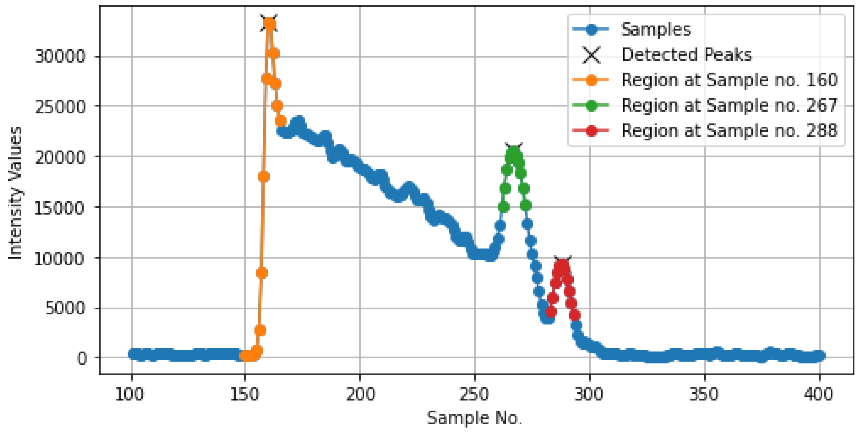
In Figure 6, based on the chosen text file, the first region (marked in orange) represents the sea surface, the second region (marked in green) is denoted as vegetation, and the third region (marked in red) is considered as the seabed. These marked regions and their intensity values were then stored and sorted for further analysis.
In this study, the classes were considered as shown below:
- Noise (Class 0)
- Sea surface (Class 1)
- Water (Class 2)
- Vegetation (Class 3)
- Seabed (Class 4)
Depending on the number of regions found, we assigned the classes as follows:
- When there were only 3 regions, the assigned classes were 1 (sea surface), 3 (vegetation), and 4 (seabed).
- When there were two regions, the assigned classes were 1 (sea surface) and 4 (Seabed), indicating no presence of vegetation.
- Lastly, upon finding four regions, the assigned classes are (1, 3, 3, 4), indicating two regions of vegetation between the sea surface and seabed.
As shown in Figure 6, the file ’waveform_303371215_ 085609_only. txt’ contains 3 distinct regions. The first region, spanning Sample_no 150-165, was defined as Class 1 (Sea Surface). The 2nd region, from Sample_no 262-272, was assigned as Class 3 (Vegetation). Finally, the 3rd region, covering Sample_no 283-293, was given as Class 4 (Seabed), as illustrated in Figure 7.
After defining the key classes (Sea surface, Vegetation, Seabed), the last step in the data preprocessing pipeline was to assign labels to the remaining intensity values. This step ensured that all intensity values in a waveform were properly classified, allowing for complete and consistent labeling of the entire 300 values from each text file. The rules to assign the remaining label were:
- The intensity values before the sea surface region and after the seabed region were assigned as class 0 (Noise).
- The intensity values between the sea surface region and the vegetation region were assigned as class 2 (Water).
- Similarly, the intensity values between the vegetation region and the seabed region were assigned as class 2 (Water).
Thus, all 300 intensity values from each waveform in the text files are classified and assigned their corresponding labels, and the individual text file is converted to CSV files alongside previously stored metadata. The distribution of these labels across classes is presented in Table 2.
3.3.4. Methodological Comparison with Existing Studies
To demonstrate the novelty of our preprocessing technique, we compared it with existing approaches that have been applied to bathymetric LiDAR data. Prior studies, such as [19,20,22], typically rely on Gaussian decomposition or manual feature extraction from point cloud representations. These methods use parameters like amplitude, echo width, and return number, and often require extensive human interpretation or simplification of the original waveform signal. In contrast, our approach processes the entire raw intensity waveform (960 samples) and applies adaptive peak detection for automatic labeling. We visualize and label each segment of the waveform based on detected peaks, supported by expert domain validation.
This methodology allows us to handle different waveform shapes and complexity levels while maintaining full signal fidelity—something that has not been adequately addressed in previous studies. Visual examples (e.g., Figure 8a–d) illustrate how our approach dynamically adapts to varying peak structures and classifies segments as sea surface, water, vegetation, seabed, or noise. Moreover, our labeling is confirmed by experts at the Norwegian Mapping Authority, which increases the credibility of our ground truth labels.
3.3.5. Feature Selection
After the data labeling steps (3.3.3), each CSV file stored a sequence of Samples (300 Intensity values) with their corresponding label, alongside the metadata stored for each file in the beginning. To improve model efficiency and eliminate redundancy, a Correlation-based Feature Selection (CFS) approach was applied. The rationale behind CFS was to identify a subset of features that:
- Have high correlation with the target variable (‘Class_Label’): Ensuring that the selected features contribute meaningful information to classification.
- Have low correlation with each other: Preventing redundancy and reducing noise in the model.
The CFS algorithm first computed the correlation between each feature and ‘Class_Label’ to determine its relevance. Next, it analyzed the intercorrelation between features to eliminate redundant information. Based on this approach, only the ‘Samples’ column was selected as the primary feature, as it demonstrated strong predictive power while minimizing redundancy from spatial coordinates and other metadata. This selection was later validated by industry experts, confirming its effectiveness in improving classification accuracy. Thus, the ‘Samples’ (intensity values) from each file were treated as an ‘X’ label (feature), and the ‘Class_Label’ was treated as a ‘Y’ label (target).
3.3.6. Data Normalization
To ensure stable training and improve model efficiency, Standardization (Z-score normalization) was applied to the ‘Samples’ using StandardScaler4. This transformation centered the data to zero mean and unit variance, preventing features with larger magnitudes from dominating the learning process. Standardization is particularly beneficial for deep learning models like LSTM, as it helps maintain stable gradient updates, reduces the risk of exploding or vanishing gradients, and accelerates convergence. Unlike Min-Max scaling, StandardScaler is more robust to outliers, making it well-suited for intensity-based bathymetric LiDAR classification.
3.3.7. One-Hot Encoding
The class label ‘Y’ needed to be in a format suitable for multi-class classification. Since the dataset contains five different classes, the labels were converted to a one-hot encoded format using the ‘to_categorical’ function. One-hot encoding transformed each label into a binary vector, where the index corresponding to the actual class was set to 1, and all other indices were set to 0. This transformation was necessary because the final output layer of the model was designed to predict class probabilities across multiple categories.
3.3.8. Splitting Data into Training, Validation, and Testing Datasets
To prepare the data for model training, 60% of the data from each dataset was allocated for training, while the remaining 20% was set aside for testing and 20% for validation purposes, ensuring effective model evaluation during training.
3.4. Model Architecture
This study employs deep learning architectures to perform multi-class classification of preprocessed Airborne LiDAR Bathymetry (ALB) waveform data into five distinct classes: sea surface, vegetation, seabed, water, and noise.
Among various neural network models, those capable of processing sequential data are particularly well-suited to modeling waveform signals, which are inherently ordered time series. One such architecture is the Long Short-Term Memory (LSTM) network. As a specialized form of Recurrent Neural Network (RNN), LSTM is designed to address the limitations of traditional RNNs, particularly the vanishing gradient problem, which hinders learning long-range dependencies in sequential data. LSTM achieves this by incorporating memory cells and three gating mechanisms—input, forget, and output gates—that regulate the flow of information through time steps. These components allow the network to selectively retain or discard information, enabling robust learning over long sequences [18,29].
LSTM has been widely applied in domains such as natural language processing, speech recognition, machine translation, and time series forecasting due to its ability to model contextual information with high temporal fidelity [30]. In this study, it is leveraged to capture waveform patterns within ALB data, where each waveform comprises 960 intensity samples representing light return strength at varying depths.
To enhance sequence comprehension further, a Bidirectional Long Short-Term Memory (BiLSTM) model is also employed. Unlike the unidirectional LSTM, which processes sequences in a single temporal direction (either past-to-future or vice versa), BiLSTM processes input sequences in both forward and backward directions. This dual-path approach allows the network to incorporate both preceding and succeeding contextual cues when making predictions, a property especially valuable in ALB data, where return signals from different surfaces (e.g., vegetation and seabed) may overlap or occur at varying depths [31,32].
While BiLSTM offers a more comprehensive contextual understanding, it comes at the cost of higher computational complexity and training time due to its dual-layered architecture. In contrast, the simpler LSTM architecture is computationally more efficient and faster to train, although it lacks access to future context during sequence processing. The comparative advantages of each model type are evaluated in this study through classification performance on the collected datasets [33].
3.4.1. LSTM Model Architecture
To multi-classify the processed ALB data into five distinct classes, the first model used was Long Short-Term Memory (LSTM). It was utilized for processing sequential input data with 300 time steps, each containing a single feature. The architecture begins with an LSTM layer of 128 units, followed by a 50% Dropout layer to mitigate overfitting. A subsequent LSTM layer with 64 units further reduces dimensionality while preserving sequence information, followed by another Dropout layer. The sequence is then transformed by a TimeDistributed Dense layer with 64 units and ReLU activation, accompanied by a final Dropout layer. The model concludes with a TimeDistributed Dense layer employing a softmax activation function, yielding per-time-step class probabilities across five categories and this is depicted in Figure 9a.
3.4.2. BiLSTM Model Architecture
The second employed model was Bidirectional Long Short-Term Memory (BiLSTM). It is designed to capture both past and future contextual information from sequential data. The input layer processed sequences of 300 time steps, each containing one feature. The first Bidirectional LSTM layer, with 128 units, encoded the sequence in both forward and backward directions, producing a concatenated output of 256 features per time step. A 50% Dropout layer is used to prevent overfitting. The second Bidirectional LSTM layer, with 64 units, further refined temporal patterns while maintaining bidirectional processing. Another Dropout layer was added to enhance model generalization. Finally, a TimeDistributed Dense layer with 5 softmax-activated units provided a per-time-step probability distribution for classification across the target classes, and this is depicted in Figure 9b. This hierarchical architecture enabled the model to learn both low-level and high-level temporal representations effectively.
While this study focuses on LSTM and BiLSTM due to their proven effectiveness in sequential data modeling, we acknowledge that alternative architectures such as GRUs, 1D CNNs with attention, and Transformer encoders have also shown strong potential in waveform-based classification tasks. For instance, [22] used a CNN-based MVCNN model on ALB waveforms, achieving 99.41% accuracy, while [9] employed a Transformer-like CNN structure for nearshore bathymetry prediction.
BiLSTM was included in our evaluation to investigate whether bidirectional temporal context could help resolve ambiguities in overlapping waveform regions (e.g., submerged vegetation). However, we recognize that the causal nature of time-of-flight laser echoes typically limits the need for backward recurrence. Our results show that LSTM outperforms BiLSTM, supporting this intuition.
A more extensive ablation study comparing LSTM, GRU, CNN+Attention, and Transformer architectures remains an important direction for future work. Such a comparison would allow for a clearer understanding of the trade-offs in accuracy, generalization, and computational efficiency when classifying ALB waveform data.
3.5. Experimental Setup and Hyperparameter Tuning
To optimize model performance across both datasets, a systematic hyperparameter tuning strategy was employed, tailored separately for the LSTM and BiLSTM architectures. The goal was to balance learning efficiency, model generalization, and training stability, while also addressing inherent challenges such as class imbalance and sequence variability.
Both models were trained using the Adam optimizer [34], known for its adaptive learning rate and computational efficiency in sparse gradient problems. The categorical cross-entropy loss function was used to guide the optimization process, given its suitability for multi-class classification tasks involving one-hot encoded labels. Models were trained for a maximum of 100 epochs, a choice informed by initial convergence analysis: training curves indicated that both models typically reached stable accuracy and loss levels well within this range, avoiding overfitting or premature termination.
LSTM Configuration: The LSTM model architecture was optimized with a batch size of 32. Initial trials explored batch sizes of 16, 32, and 64. While smaller batch sizes tended to overfit faster and larger sizes slowed convergence, a batch size of 32 provided the best trade-off between learning stability and gradient update frequency. The model included a dropout layer with a rate of 0.5 to mitigate overfitting, especially due to the sequential nature of the waveform input. A total of 64 LSTM units were used based on empirical testing, with no substantial gain observed for higher values.
BiLSTM Configuration: Due to the increased complexity and bidirectional nature of BiLSTM, a batch size of 16 was selected. This smaller batch size was beneficial for ensuring gradient stability and convergence, particularly when processing both forward and backward sequences simultaneously. Additionally, class imbalance—especially underrepresentation of vegetation and seabed classes (labels 3 and 4)—posed a significant challenge. To address this, dynamic class weights were computed based on the frequency distribution of the training labels. These weights were incorporated into the model’s loss function, ensuring that minority classes contributed more prominently during training. Table 3 presents the calculated weights applied to each class.
Model Comparison: While both LSTM and BiLSTM share core architectural principles, the differences in processing direction, batch size, and class imbalance treatment had a notable impact on performance. Table 4 summarizes these distinctions, highlighting key design choices, such as the use of weighted loss for BiLSTM and unweighted loss for LSTM, and architectural differences that influence training behavior and computational complexity.
This tuning strategy, combining empirical observation with performance-driven iteration, ensured that both models were optimally configured for handling the sequential nature of ALB waveform data and the classification of underwater features with high fidelity.
For transparency and reproducibility, the hyperparameters were tuned using a manual grid search strategy. Specifically, we evaluated learning rates (1e-3, 1e-4), batch sizes (16, 32, 64), and dropout rates (0.3, 0.5), selecting the best combination based on validation accuracy and F1-score. Both models were trained using the Adam optimizer for a maximum of 100 epochs, with early stopping (patience = 10) applied to prevent overfitting. A fixed random seed (42) was used across all experiments to ensure reproducibility. All computations were performed on a personal computer equipped with an Intel(R) Iris(R) Xe integrated GPU, 16GB RAM, and Windows 11. Training and evaluation were conducted using CPU-based processing over a total wall-clock budget of approximately 48 hours. The best-performing configurations are summarized in Table 4.
3.6. Model Performance Metrics
Model performance is a measure of how well a model does the task it is intended to do. In the case of classification models, which have discrete outputs, performance metrics compare the predicted classes with the actual classes. It enables us to show the model’s error in different aspects and their contribution to predictions. [35,36]. This section elaborates on the traditional performance metrics that can help justify how well the deep learning model is performing based on the test dataset. The performance of the final models was assessed using key evaluation metrics, including the confusion matrix, accuracy, precision, recall, and F1-score, to offer a comprehensive analysis of their classification capabilities.
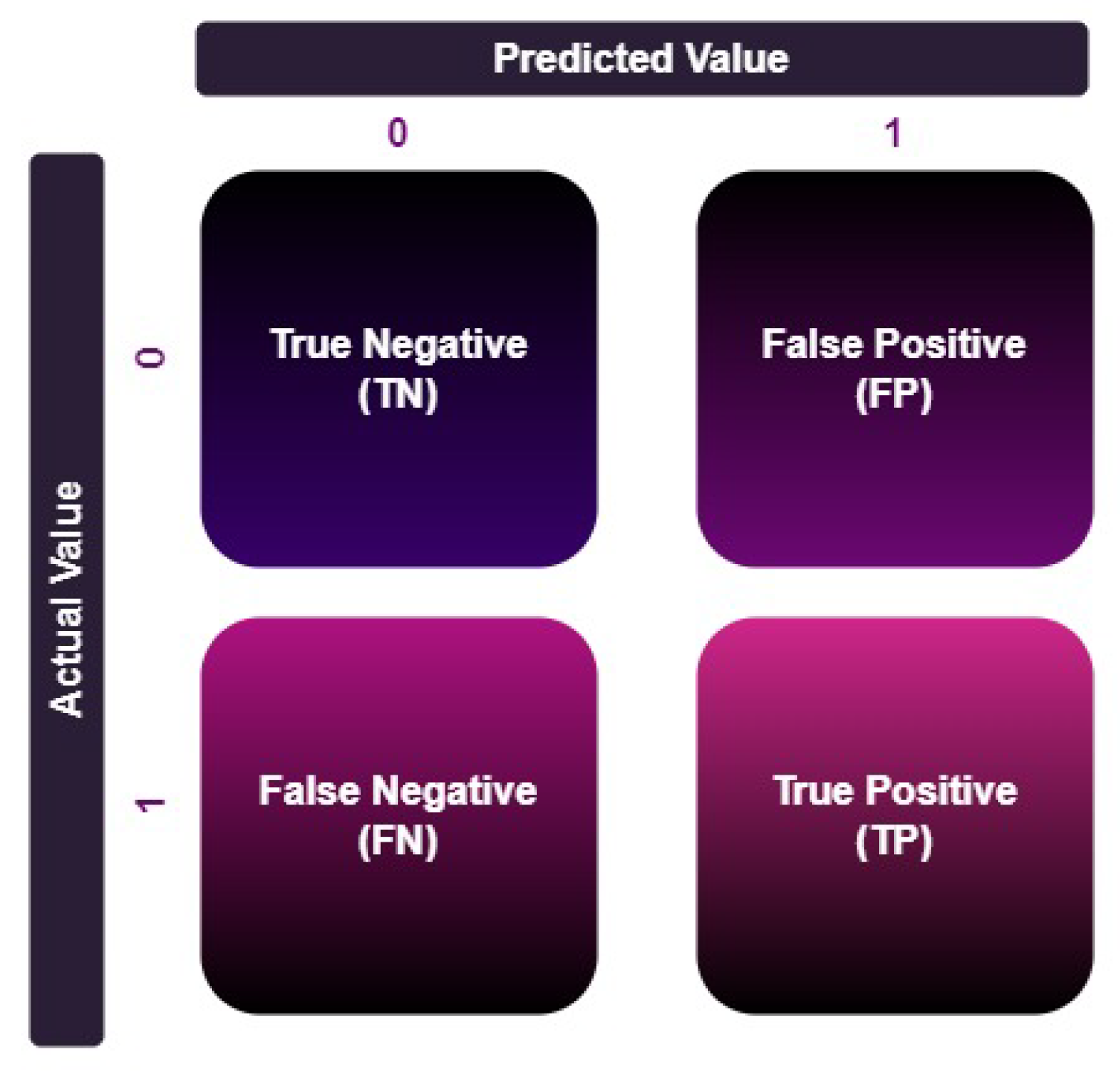
As the classification tasks predict discrete classes, evaluating the correctness of these predictions requires the breakdown of the outcomes. These outcomes are represented as [37]:
- True Positives (TP): Positive cases that are correctly predicted.
- True Negatives (TN): Negative cases that are correctly predicted.
- False Positives (FP): Negative cases that are incorrectly predicted as positive (also known as Type I error)
- False Negatives (FN): Positive cases that are incorrectly predicted as negative (also known as Type II error).
These basic building blocks help explain the different ways performance can be assessed in classification models. The Confusion Matrix is a valuable tool for organizing this information, showing how the model performs in predicting each class and laying the groundwork for calculating performance metrics like Precision, Recall, F1-Score, and Accuracy [35].
Figure 10.
Confusion Matrix.
3.6.1. Accuracy
3.6.2. Precision
Precision measures the proportion of true positives among all predicted positives. It reflects the model’s ability to avoid false positives. A low Precision score (<0.5) indicates a high number of false positives, which can be caused by imbalance or untuned model parameters. Precision is particularly important in applications where false positives are costly, such as in spam detection [35]. The following formula is used to calculate precision.
3.6.3. Recall
Recall measures the proportion of true positives among all actual positives. It is also known as sensitivity or true positive rate (TPR). It evaluates how well the model identifies all relevant instances of the positive class. It is important in scenarios where missing positive cases is more critical than incorrectly identifying negatives. A high Recall ensures that as many true positive cases as possible are identified. However, low Recall (<0.5) suggests that the model is missing many true positives [35,38]. The following formula is used to calculate recall.
3.6.4. F1-Score
The F1-score is a statistic that offers a balance between Precision and Recall, defined as the harmonic mean of these two variables. It is very helpful in imbalanced classification problems and other scenarios where minimizing false positives and false negatives is necessary. In many real-world scenarios, an F1-score is a more credible indicator than Accuracy because it shows that the model is performing well in both Precision and Recall [35,38]. The following formula is used to calculate the F1-Score.
3.6.5. Confusion Matrix
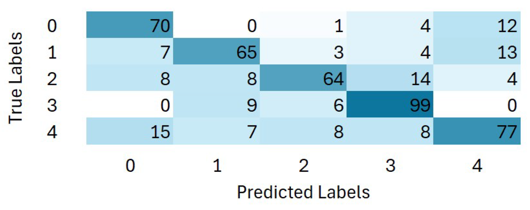
Figure 11 represents the confusion matrix, offering a structured representation of the multi-class classification models’ performance. In this study, the matrix encompasses five classes, each representing a distinct category within the datasets. This highlights a model’s performance by displaying the distribution of accurate and inaccurate predictions for every class. It allows for a detailed analysis of errors. This helps to identify which specific classes the model struggles with. The model’s weaknesses may come from false positives, false negatives, or a combination. The matrix, for instance, enables us to determine if a model consistently predicts one class over another or misclassified particular kinds of cases [35,38].
Figure 11.
Confusion Matrix of Multi-Class Classification.
4. Results
This section presents the results obtained from various experiments using both datasets. The results will be presented separately for each dataset. For each dataset, the results from the LSTM model will be presented first, followed by the results from the BiLSTM model.
4.1. Results on the Dataset 1
Two deep learning models, LSTM and BiLSTM, were employed to perform multi-class classification on airborne bathymetric waveform data. The results obtained from the LSTM model are presented in Figure 12a. As shown in the figure and Table 5, the LSTM model achieved an accuracy of 95.22%, with a macro average precision score of 0.8787, a recall score of 0.8594, and an F1-score of 0.8641. The weighted average precision score of 0.9533, recall score of 0.9522, and F1-score of 0.9518 for Dataset 1.
Figure 12.
The Obtained Accuracy Results and Confusion Matrix on Dataset 1.
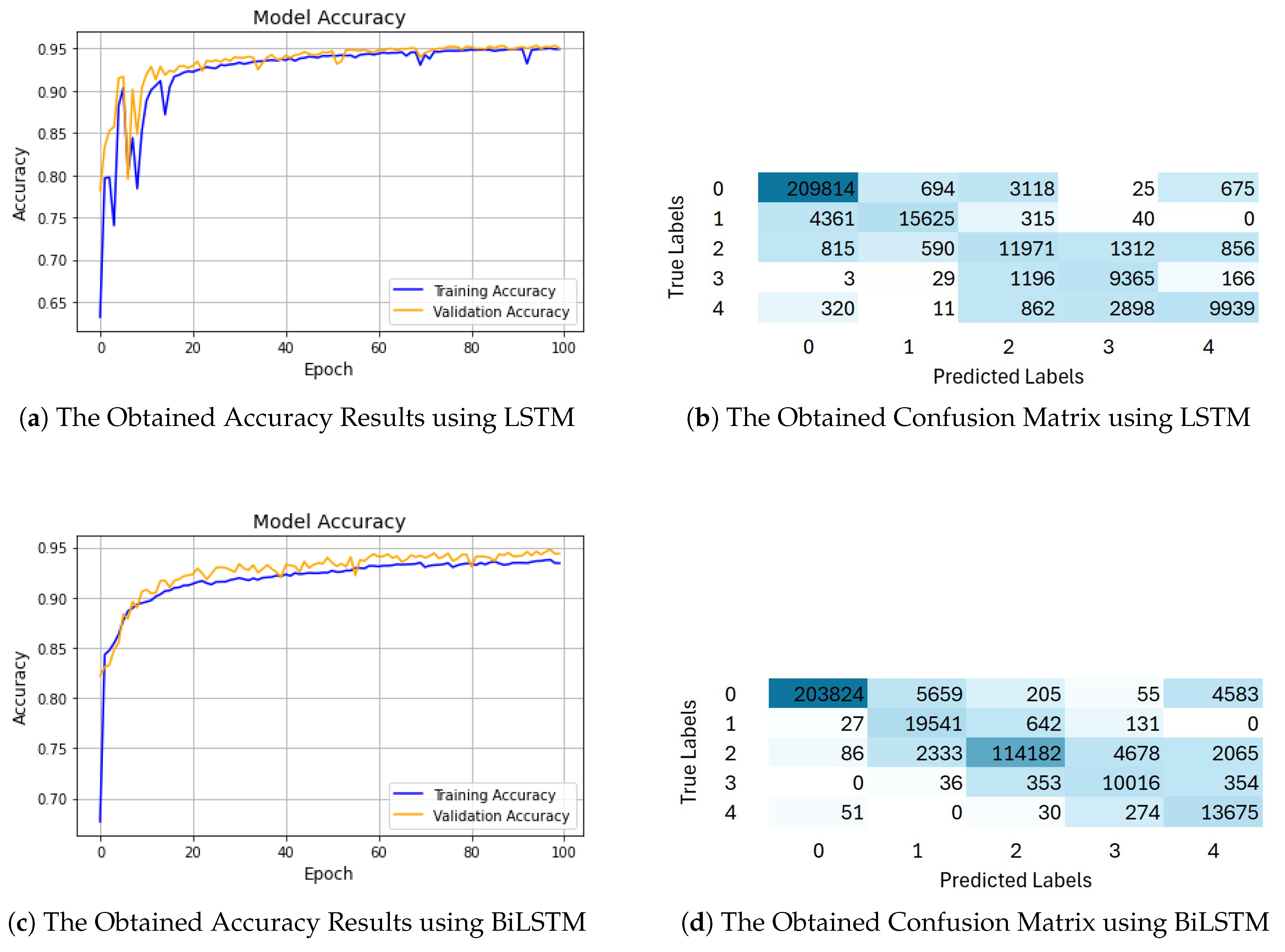
The confusion matrix analysis, illustrated in Figure 12b, demonstrates the performance of the LSTM model for each class. It highlights the dominance of the diagonal elements, indicating correct classifications, over the off-diagonal elements, which represent misclassifications. Notably, the model correctly classified 209,814 out of 214,326 instances of noise (class 1). However, 694 instances were misclassified as sea surface (class 1), 675 as seabed (class 4), and 3,118 as water (class 2). These misclassifications are minimal compared to the high number of correct predictions, showcasing the model’s robustness in filtering out noise.
For class 1 (Sea Surface), the model correctly classified 15,625 instances out of 20,341 instances. There were 4,361 instances of sea surface misclassified as noise (class 0), and 315 instances as water (class 2). The water class was classified with excellent accuracy, correctly identifying 119,771 out of 123,344 instances. However, 1,312 were misclassified as vegetation (class 3), and 856 were as seabed (class 4), indicating the challenge of distinguishing these features in shallow or turbulent regions where water, vegetation, and seabed characteristics can blend. For class 3 (Vegetation), the model accurately classified 9365 out of 10,759 instances, with 1,196 misclassified as water (class 2). For class 4 (Seabed), the model correctly classified 9,939 instances out of 14,030 instances, with 2,898 misclassified as vegetation (class 3). The overlap between seabed and vegetation is likely due to similarities in waveform profiles near the sea bottom, where vegetation is present.
The results obtained using the BiLSTM model are presented in Figure 12c. As shown in this figure and Table 5, the employed model demonstrates strong performance in the classification tasks, achieving an accuracy of 94.85%, with a macro average precision score of 0.8039, recall score of 0.9486 and F1-score of 0.8616. The weighted average precision score of 0.9587, recall score of 0.9437, and F1-score of 0.9478 on Dataset 1.
The confusion matrix analysis, depicted in Figure 12d, highlights both the strengths and weaknesses of the BiLSTM model. For class 0 (Noise), the model accurately classified 203,824 instances out of 214,326 instances. However, 5659 instances were misclassified as sea surface (class 1), and 4583 instances were incorrectly identified as seabed (class 4). These misclassifications can be attributed to the complexity of distinguishing noise from the actual sea surface and seabed features, especially in regions with mixed or unclear signals.
For class 1 (Sea Surface), the model correctly identified 19,541 out of 20,341 instances. It misclassified 642 instances as water (class 2), and 131 as vegetation (class 3). This misclassification of the sea surface as water could arise due to similar waveform patterns in shallow coastal regions, where the sea surface and water might blend. Similarly, the misclassification as vegetation is likely due to similar signal characteristics between the sea surface and areas with dense vegetation. For class 2 (Water), the model accurately classified 114,182 out of 123,344 water instances. Despite this, 4,678 instances were misclassified as vegetation (class 3), and 2333 as sea surface (class 1). These misclassifications could be due to overlapping characteristics of water and vegetation, especially in regions where vegetation is submerged or near the water surface, leading to confusion between the two classes. For class 3 (Vegetation), the model correctly classified 10,016 out of 20759 as vegetation. However, it misclassified 353 instances as water (class 2), and 354 as seabed (class 4). These misclassifications may be due to the presence of submerged vegetation that shares similar waveform profiles with water or seabed features. Finally, for class 4 (Seabed), the model correctly classified 13,675 instances out of 14,030, with 274 instances misclassified as vegetation (class 3). This misclassification likely results from the overlapping characteristics of the seabed and vegetation, especially in regions where the seabed contains vegetation-like features, such as seagrasses or algae, which could have confused the model.
4.2. Results on the Dataset 2
The results obtained from the LSTM model on Dataset 2 are shown in Figure 13a. As illustrated in this figure and Table 5, the LSTM model achieved an accuracy of 94.85% with a macro average precision score of 0.7011, a recall score of 0.6885, and an F1-score of 0.6945. The obtained weighted average precision score of 0.9446, the recall score of 0.9485, and the F1-score of 0.9464.
Figure 13.
The Obtained Accuracy Results and Confusion Matrix on Dataset 2.
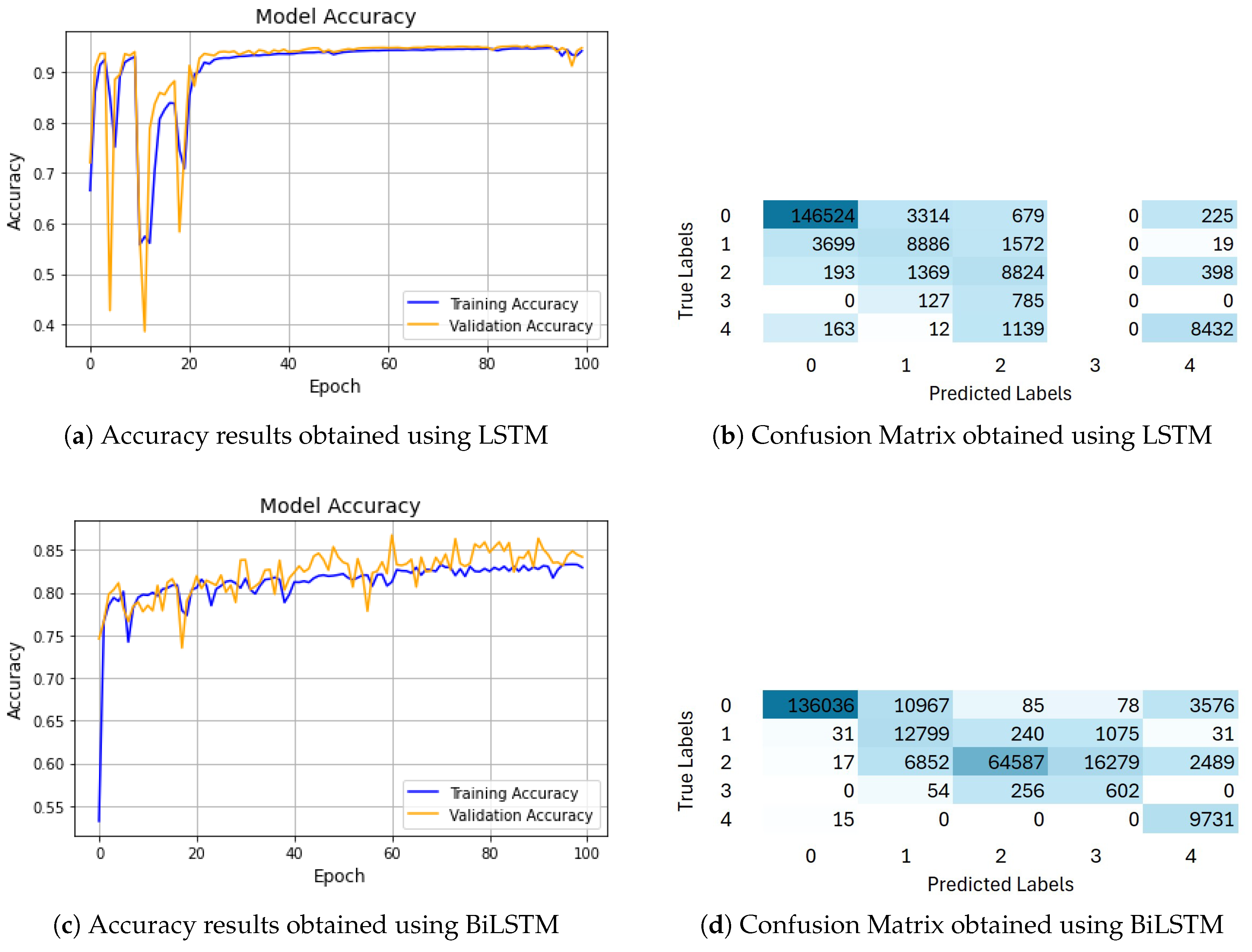
The obtained Confusion Matrix analysis is depicted in Figure 13b. From this figure, it can be observed that for class 0 (Noise), the model correctly classified 146,524 instances out of 150,742. However, 3,314 instances were misclassified as Class 1, 679 instances as Class 2, and 225 as Class 4. For class 1 (Sea Surface), the model accurately classified 8886 out of 14,176 instances. Misclassifications included 3,699 instances as Class 0, 1,572 instances as Class 2, and 19 as Class 4. For class 2 (Water), the model correctly classified 88,264 out of 90,224 instances. Nonetheless, 1,369 instances were misclassified as Class 1, 193 instances as Class 0, and 398 instances as Class 4. For class 3 (Vegetation), the model faced challenges, correctly classifying 0 out of 912 instances. The remaining 785 instances were misclassified into Class 2, and 127 instances as Class 1. Finally, for class 4 (Seabed), the model correctly classified 8,432 out of 9,746 instances. However, 1,139 instances were misclassified as Class 2, 163 instances as Class 0, and 12 as Class 1. These misclassifications can be attributed to overlapping features between the classes, particularly in instances where the characteristics of noise, sea surface, and water classes are similar. Furthermore, the model struggled to classify vegetation (Class 3) due to the ambiguity between vegetation and water, especially in shallow or turbulent regions, as well as the complexity of distinguishing between seabed and vegetation in certain waveform profiles near the seabed.
When applying the BiLSTM model to Dataset 2, the results obtained are presented in Figure 13c. From this figure and Table 5, it can be observed that the model achieved an accuracy of 84.18%, with a macro average: precision score of 0.6112, recall score of 0.8359, and F1-score of 0.635. The weighted average for the model’s performance was: precision score of 0.9482, recall score of 0.8418, and F1-score of 0.8787 on Dataset 2.
The confusion matrix analysis (see Figure 13d) highlights both the strengths and weaknesses of the BiLSTM model. For class 0 (Noise), the model correctly classified 136,036 instances out of 150,742, but 10,967 instances were misclassified as Class 1, and 3,576 instances as Class 4. For class 1 (Sea Surface), the model correctly classified 12,799 out of 14176, while 1,075 were misclassified as Class 3, and 240 instances as Class 2. For class 2 (Water), the model accurately classified 64,587 out of 90,224 instances, with 16,279 instances misclassified as Class 3, and 6,852 as Class 1. In Class 3 (Vegetation), the model correctly classified 602 out of 912 instances, but 256 were misclassified as Class 2, and 54 as Class 1. Finally, for class 4 (Seabed), the model performed well, correctly classifying 9,731 out of 9,746 instances, with only minimal misclassification.
These aforementioned misclassifications can be attributed to several factors. The confusion between noise and other classes (Class 1 and Class 4) may stem from the similar characteristics in certain waveform profiles. In addition, the misclassification of water and vegetation could be due to their overlapping features, especially in shallow or vegetated areas, which makes it difficult for the model to distinguish them accurately. Furthermore, the model faced challenges in classifying vegetation correctly, likely due to its mixed signal characteristics with water and seabed classes, particularly in regions where vegetation growth blends with water or seabed features.
4.3. Results on Reliability Analysis Using Confidence Scores
To assess the reliability of classification for each sample, a confidence score was calculated for each predicted class. This score indicates the level of certainty associated with classifying a specific sample in a waveform, addressing Research Question 2 (2). For illustration, the confidence score of a specific waveform from Dataset 1 is discussed here. The results for both models are presented in Figure 14 and Figure 15. These figures provide insights into the reliability of classification for each sample, helping to understand how confidently each specific point was classified.
Figure 14.
The Confidence Score for a specific file using LSTM from Dataset 1.
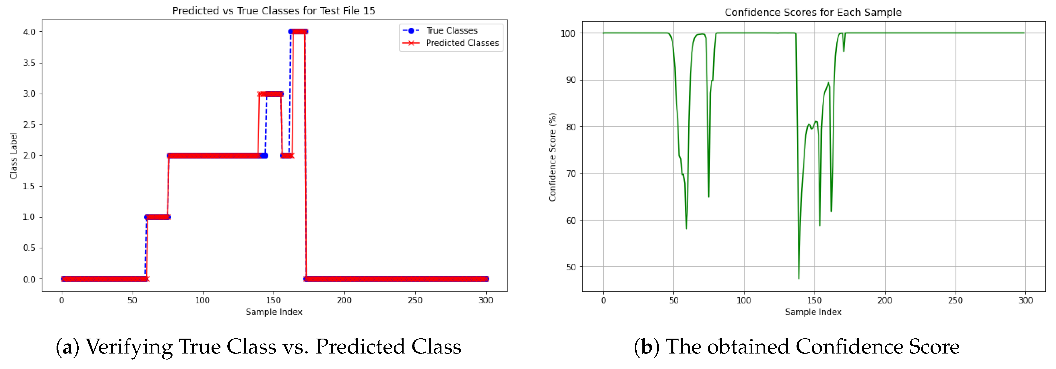
Figure 15.
The Confidence Score for a specific file using BiLSTM from Dataset 1.
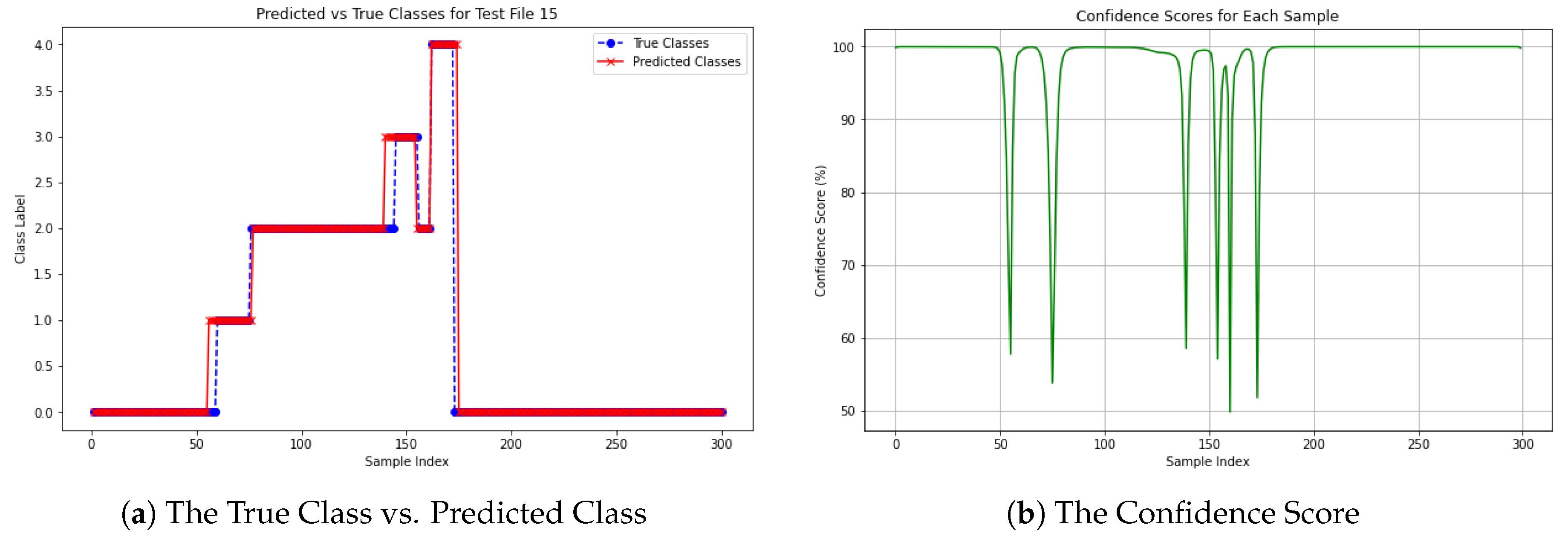
Figure 14a shows the comparison between the True Vs Predicted Class labels for each of the 300 samples. The true class labels are represented by blue dots, while the predicted class labels are shown as red markers. In general, the predicted classes align well with the true classes, as evidenced by the overlapping points throughout most of the graph. However, deviations between the predicted and true classes were observed around sample indices 130-160, which corresponded to dips in the confidence score chart shown in Figure 14b. Overall, the model performed effectively on this waveform, with most predictions matching the true labels, except for the misclassified instances between indices 130-160, where the confidence scores were notably lower.
Figure 15a displays the comparison between the True Vs Predicted Class labels from the same waveform from Dataset 1, obtained using the BiLSTM model. The graph demonstrates that, in most sections, the predicted classes closely align with the true classes, showing minimal divergence and suggesting strong model performance. However, noticeable deviations can be observed between sample indices 130 to 140, where the true and predicted classes differ. For a clearer visualization, the confidence score for the 300 samples in this file is shown in Figure 15b.
From the analysis, it can be concluded that both models experience significant confidence dips on certain samples, with minimum scores around 47% (LSTM) and 50% (BiLSTM). While their overall performance is similar, BiLSTM shows a slight edge in consistency during these dips, likely due to its bidirectional structure, which captures context from both directions. Although there is no definitive answer to this research question, the confidence score provides a probabilistic measure of the model’s certainty for each classification. This is particularly important for tasks that require precise seabed and vegetation mapping.
5. Discussion
This study proposed a novel approach for classifying Airborne LiDAR Bathymetry (ALB) waveform data using deep learning models, specifically Long Short-Term Memory (LSTM) and Bidirectional LSTM (BiLSTM) networks. By processing the full waveform sequence (960 intensity samples) as input, the method avoids the need for handcrafted features, Gaussian decomposition, or point cloud geometry. Instead, it applies a peak detection-based preprocessing pipeline and sequence modeling to classify each waveform into five distinct classes: sea surface, water, vegetation, seabed, and noise.
While BiLSTM models are designed to capture both past and future temporal dependencies, their applicability to airborne bathymetric LiDAR waveform data is not straightforward. ALB waveforms are generated by time-of-flight laser signals, which are inherently unidirectional in nature—each return represents a causal sequence of interactions from sea surface to seabed. Including BiLSTM in this study aimed to investigate whether backward recurrence could help disambiguate overlapping or noisy waveform segments, particularly in complex cases like submerged vegetation.
However, the results indicate that LSTM consistently outperformed BiLSTM on both datasets. This suggests that the added complexity and bidirectional processing did not provide meaningful advantages for this specific data type. Instead, it may have introduced unnecessary computation and confusion in scenarios where future context is not physically meaningful. These findings reinforce the appropriateness of using unidirectional models for time-of-flight data and highlight the importance of aligning model architecture with signal properties.
Misclassification between the water and vegetation classes was observed in both models. This is likely due to overlapping waveform signatures that occur when submerged vegetation mimics the intensity return characteristics of shallow water. These overlaps make it difficult for models to distinguish between the two classes based solely on sequence information. To mitigate this challenge, future research could explore data balancing techniques such as Synthetic Minority Over-sampling Technique (SMOTE) or data augmentation to strengthen the model’s ability to learn from underrepresented waveform patterns. Such approaches have been shown to improve minority class detection in previous LiDAR classification studies [20].
A key strength of this study lies in its expert-validated ground truthing process. The labeling of waveforms was conducted in collaboration with domain experts at the Norwegian Mapping Authority. Waveforms were visually examined and categorized into seabed, vegetation, and sea surface classes based on intensity peak structure and expert knowledge. This expert-informed labeling was used to train the deep learning models and evaluate their predictions through precision, recall, F1-score, and confusion matrix analysis. Although cross-validation was not applied due to the structured nature of the dataset and expert-defined splits, the evaluation metrics and visual analysis offer robust support for the reliability of the results.
Another factor affecting model performance, particularly in the second dataset, was the imbalance in class distribution, most notably the limited number of vegetation-labeled waveforms. The second dataset contained significantly fewer vegetation samples compared to the first, resulting in the underrepresentation of this class during training. This lack of training data led to reduced model exposure to vegetation-specific waveform patterns, which likely contributed to the drop in classification accuracy for that class. As deep learning models are heavily dependent on diverse and balanced training data to learn generalizable features, the vegetation class suffered from reduced precision and recall in the second dataset. This observation highlights the importance of dataset balance and suggests that future work should include synthetic oversampling, such as SMOTE, or additional data collection to ensure consistent representation across all classes.
When comparing our results to existing literature, our approach stands out for its simplicity and scalability. Prior studies have used Multi-Layer Perceptrons (MLP), PointNet, or Convolutional Neural Networks (CNN) for classification tasks, but often depended on spatial context, handcrafted features, or additional geometric parameters to boost performance. In contrast, our method relies solely on full waveform sequences and does not require spatial neighborhood information or manual feature extraction. As shown in Table 1, this streamlined approach not only reduces preprocessing overhead but also achieves strong classification results using raw ALB signals.
Environmental factors, such as water turbidity, depth, and wave motion, are known to significantly influence the quality and structure of LiDAR waveforms. For instance, high turbidity can attenuate the green laser signal, reducing penetration depth and blurring peak intensities, while shallow waters with surface motion can cause waveform distortion. These effects likely contributed to the model’s performance variability, especially the lower accuracy for the vegetation class in Dataset 2, which had fewer samples and potentially more environmental variability. Although this study did not explicitly incorporate environmental metadata due to limited availability, we recognize that modeling these conditions is essential for improving generalizability. Future work could stratify model performance by depth or turbidity bins, or use correlation plots to link prediction confidence with environmental conditions. Additionally, integrating auxiliary sensor metadata—such as scan angle, bottom reflectance, or return waveform shape—could help the model disambiguate class boundaries in environmentally complex regions. Adaptive preprocessing or feature engineering informed by environmental context may also reduce misclassification in overlapping waveform regions.
In summary, this study contributes a novel, expert-informed full waveform classification pipeline using deep learning, validates its effectiveness through comparative experiments, and offers practical insights for improving ALB-based subsea mapping. The proposed method not only fills a gap in the literature by directly using full waveform data but also sets the stage for more scalable, robust, and cost-effective solutions in the field of marine geospatial analysis.
6. Conclusions and Future Work
Airborne bathymetric LiDAR (ALB) has emerged as a transformative technology for underwater mapping, especially in shallow water and transitional zones where traditional methods like Multibeam Echosounders (MBES) face limitations. ALB’s ability to measure depths up to 30 meters and efficiently capture detailed subsea features makes it a critical tool for modern seabed mapping. However, the vast volume and complexity of ALB data pose significant challenges for real-time processing and accurate classification. This study investigated the effectiveness of deep learning models, specifically LSTM and BiLSTM, in classifying ALB data into five classes, such as sea surface, seabed, vegetation, water, and noise.
The LSTM model proved to be the superior choice for classifying airborne bathymetric LiDAR (ALB) waveforms, achieving 95.22% accuracy on Dataset 1 and 94.85% on Dataset 2, outperforming BiLSTM, which dropped to 84.18% on Dataset 2. This higher accuracy ensures a more reliable classification of seabed, vegetation, and water surfaces, which is critical for safe navigation.
LSTM also demonstrated better precision (87.87% vs. 80.39% on Dataset 1, 70.11% vs. 61.12% on Dataset 2), meaning fewer false detections that could mislead navigation systems. While BiLSTM had a slightly higher recall on Dataset 1 (94.86%), it struggled on Dataset 2, where LSTM maintained a more balanced recall (85.94% on Dataset 1, 68.85% on Dataset 2).
Given its higher accuracy, better precision, and balanced recall, LSTM is the preferred model for maritime navigation. It ensures fewer false detections while reliably identifying key underwater features, making it a more dependable solution for safe and efficient seabed mapping.
Despite these promising results, challenges remain. The models exhibited sensitivity to noise, misclassification of overlapping classes, and high computational demands, particularly in BiLSTM. Future research could explore hybrid models integrating LSTM/BiLSTM with attention mechanisms or spectral data to refine classification performance further. Transformer-based architectures also present a promising avenue for capturing complex temporal and spatial relationships in ALB data.
To advance the integration of ALB into modern seabed mapping workflows, future work should focus on enhancing real-time processing capabilities and improving uncertainty quantification through probabilistic modeling or ensemble learning approaches. These advancements will not only increase the reliability of predictions but also build greater confidence in ALB-based products, supporting safer navigation and more effective marine ecosystem management. Addressing these challenges will solidify deep learning-based ALB classification as a pivotal tool in next-generation underwater mapping solutions.
The suggested approach does not specifically take environmental parameters like water depth, turbidity, or surface wave motion into consideration, yet it shows good classification performance on ALB waveform data. The quality of LiDAR returns can be greatly impacted by these factors. High amounts of turbidity, for instance, can attenuate or scatter the green laser signal, decreasing penetration and changing the shape of the waveform. Similarly, especially in shallow waters, wave-induced surface motion may cause noise or distort the return signal, which could result in incorrect classification. Future research could address these environmental factors by using sensor-specific metadata like scan angle and return intensity, or auxiliary data like tide levels and water clarity indexes.
Author Contributions
Conceptualization, N.T., H.G, V.M. and I.O.; methodology, N.T., H.G, V.M. and I.O.; software, N.T; validation, N.T., V.M. and I.O.; formal analysis, N.T; investigation, N.T; data curation, N.T; writing—original draft preparation, N.T; writing—review and editing, N.T., H.G, V.M. and I.O.; visualization, N.T.; supervision, H.G, V.M. and I.O. All authors have read and agreed to the published version of the manuscript.
Funding
This research received no external funding.
Institutional Review Board Statement
Not applicable.
Data Availability Statement
The dataset used in this study, alongside the necessary scripts for model training, can be found in this GitHub repository: Classification of Bathymetric Data 2024.
Acknowledgments
The authors thank the Norwegian Mapping Authority for its support in providing resources and access to data, which have been instrumental in advancing this research. This study is the result of a 60-ECTS master’s thesis in Computer Science at the Department of Science and Industry Systems, Faculty of Technology, Natural Sciences and Maritime Sciences, University of South-Eastern Norway (USN), Kongsberg, Norway.
Conflicts of Interest
The authors declare no conflicts of interest.
Abbreviations
The following abbreviations are used in this manuscript:
| ALB | Airborne LiDAR Bathymetry |
| ALS | Airborne Laser Scanning |
| BiLSTM | Bidirectional Long Short-Term Memory |
| CNN | Convolutional Neural Network |
| DL | Deep Learning |
| LiDAR | Light Detection and Ranging |
| LSTM | Long Short-Term Memory |
| MBES | Multi-Beam Echo Sounders |
| MLP | Multi-Layer Perceptron |
| NMA | Norwegian Mapping Authority |
| RF | Random Forest |
| RNN | Recurrent Neural Network |
| SMOTE | Synthetic Minority Oversampling Technique |
| SVM | Support Vector Machine |
References
- UNESCO Ocean Literacy. The List of the Oceans with data and statistics about surface area, volume, and average depth, 2022. Available online: https://oceanliteracy.unesco.org/ocean/ (accessed on 9 December 2024).
- IFAW. How climate change impacts the ocean, 2024. Available online: https://www.ifaw.org/international/journal/climate-change-impact-ocean (accessed on 27 December 2024).
- United Nations. Transforming our world: The 2030 Agenda for Sustainable Development, 2015. Available online: https://sdgs.un.org/2030agenda (accessed on 12 January 2025).
- World Ocean Review. Transport over the seas, 2024. Available online: https://worldoceanreview.com/en/wor-7/transport-over-the-seas/ (accessed on 27 September 2024).
- American Scientist. An Ocean of Reasons to Map the Seafloor, 2023. Available online: https://www.americanscientist.org/article/an-ocean-of-reasons-to-map-the-seafloor (accessed on 4 September 2024).
- Thorsnes, T.; Misund, O.A.; Smelror, M. Seabed mapping in Norwegian waters: Programmes, technologies and future advances. 499, 99–118. Publisher: The Geological Society of London. [CrossRef]
- Kartverket. Om Kartverket, 2023. Available online: https://kartverket.no/om-kartverket (accessed on 6 September 2023).
- Daniel, S.; Dupont, V. Investigating Fully Convulutional Network To Semantic Labelling Of Bathymetric Point Cloud. V-2-2020, 657–663. Conference Name: XXIV ISPRS Congress, Commission II (Volume V-2-2020) - 2020 edition Publisher: Copernicus GmbH. [CrossRef]
- Zhong, J.; Sun, J.; Lai, Z.; Song, Y. Nearshore Bathymetry from ICESat-2 LiDAR and Sentinel-2 Imagery Datasets Using Deep Learning Approach. 14, 4229. Number: 17 Publisher: Multidisciplinary Digital Publishing Institute. [CrossRef]
- Janowski, L.; Wroblewski, R.; Rucinska, M.; Kubowicz-Grajewska, A.; Tysiac, P. Automatic classification and mapping of the seabed using airborne LiDAR bathymetry. 301, 106615. [CrossRef]
- Pricope, N.; Bashit, M.S. Emerging trends in topobathymetric LiDAR technology and mapping. 44, 7706–7731. [CrossRef]
- Szafarczyk, A.; Toś, C. The Use of Green Laser in LiDAR Bathymetry: State of the Art and Recent Advancements. 23, 292. Number: 1 Publisher: Multidisciplinary Digital Publishing Institute. [CrossRef]
- Dolan, M.; Buhl-Mortensen, P.; Thorsnes, T.; Buhl-Mortensen, L.; Bellec, V.; Bøe, R. Developing seabed nature-type maps offshore Norway: Initial results from the MAREANO programme. Norwegian Journal of Geology 2009, 89, 17–28. [Google Scholar]
- Leica Geosystems. Mapping underwater terrain with bathymetric LiDAR, 2024. Available online: https://leica-geosystems.com/case-studies/natural-resources/mapping-underwater-terrain-with-bathymetric-lidar (accessed on 4 September 2024).
- Li, Z.; Chen, B.; Wu, S.; Su, M.; Chen, J.M.; Xu, B. Deep learning for urban land use category classification: A review and experimental assessment. 311, 114290. [CrossRef]
- Saleh, A.; Sheaves, M.; Jerry, D.; Rahimi Azghadi, M. Applications of deep learning in fish habitat monitoring: A tutorial and survey. 238, 121841. [CrossRef]
- Tabassum, N.; Giudici, H.; Nunavath, V. Exploring the Combined use of Deep Learning and LiDAR Bathymetry Point-Clouds to Enhance Safe Navigability for Maritime Transportation: A Systematic Literature Review. In Proceedings of the 2024 Sixth International Conference on Intelligent Computing in Data Sciences (ICDS), 2024, pp. 1–5. [CrossRef]
- Restackio. Deep Learning Techniques for Sequential Data, 2024. Available online: https://www.restack.io/p/sequence-to-sequence-models-answer-deep-learning-techniques-sequential-data-cat-ai (accessed on 28 October 2024).
- Kogut, T.; Weistock, M.; Bakuła, K. Classification Of Data From Airborne LiDAR Bathymetry With Random Forest Algorithm based on Different Feature Vectors. XLII-2-W16, 143–148. Conference Name: Photogrammetric Image Analysis & Munich Remote Sensing Symposium: Joint ISPRS conference (Volume XLII-2/W16) - 18-20 September 2019, Munich, Germany Publisher: Copernicus GmbH. [CrossRef]
- Kogut, T.; Tomczak, A.; Słowik, A.; Oberski, T. Seabed Modelling by Means of Airborne Laser Bathymetry Data and Imbalanced Learning for Offshore Mapping. 22, 3121. Number: 9 Publisher: Multidisciplinary Digital Publishing Institute. [CrossRef]
- Roshandel, S.; Liu, W.; Wang, C.; Li, J. Semantic Segmentation of Coastal Zone on Airborne Lidar Bathymetry Point Clouds. 19, 1–5. Conference Name: IEEE Geoscience and Remote Sensing Letters. [CrossRef]
- Liang, G.; Zhao, X.; Zhao, J.; Zhou, F. MVCNN: A Deep Learning-Based Ocean–Land Waveform Classification Network for Single-Wavelength LiDAR Bathymetry. 16, 656–674. [CrossRef]
- Kogut, T.; Weistock, M. Classifying airborne bathymetry data using the Random Forest algorithm. 10, 874–882. [CrossRef]
- Pan, S.; Yoshida, K. Using Airborne Lidar Bathymetry Aided Transfer Learning Method in Riverine Land Cover Classification. Conference Name: 14th International Symposium on Ecohydraulics (2022, Nanjing).
- Eren, F.; Pe’eri, S.; Rzhanov, Y.; Ward, L. Bottom characterization by using airborne lidar bathymetry (ALB) waveform features obtained from bottom return residual analysis. 206, 260–274. [CrossRef]
- Wikipedia contributors. Fjøløy, 2023. Available online: https://en.wikipedia.org/w/index.php?title=Fj%C3%B8l%C3%B8y&oldid=1155343996 (accessed on 10 September 2024).
- Terrasolid. Waveform Processing, 2023. Available online: https://terrasolid.com/guides/tscan/introwaveformprocessing.html (accessed on 12 December 2023).
- Xiong, H.; Pandey, G.; Steinbach, M.; Kumar, V. Enhancing data analysis with noise removal. 18, 304–319. Conference Name: IEEE Transactions on Knowledge and Data Engineering. [CrossRef]
- Anishnama. Understanding LSTM: Architecture, Pros and Cons, and Implementation, 2023. Available online: https://medium.com/@anishnama20/understanding-lstm-architecture-pros-and-cons-and-implementation-3e0cca194094 (accessed on 29 September 2024).
- GeeksforGeeks. What is LSTM - Long Short Term Memory?, 2019. Available online: https://www.geeksforgeeks.org/deep-learning-introduction-to-long-short-term-memory/ (accessed on 29 September 2024).
- Anishnama. Understanding Bidirectional LSTM for Sequential Data Processing, 2023. Available online: https://medium.com/@anishnama20/understanding-bidirectional-lstm-for-sequential-data-processing-b83d6283befc (accessed on 30 October 2024).
- Saturn Cloud. Bidirectional LSTM, 2023. Available online: https://saturncloud.io/glossary/bidirectional-lstm/ (accessed on 30 October 2024).
- GeeksforGeeks. Difference Between a Bidirectional LSTM and an LSTM, 2024. Available online: https://www.geeksforgeeks.org/difference-between-a-bidirectional-lstm-and-an-lstm/ (accessed on 3 November 2024).
- Brownlee, J. Gentle Introduction to the Adam Optimization Algorithm for Deep Learning, 2017. Available online: https://www.machinelearningmastery.com/adam-optimization-algorithm-for-deep-learning/ (accessed on 3 November 2024).
- Bajaj, A. Performance Metrics in Machine Learning, 2022. Available online: https://neptune.ai/blog/performance-metrics-in-machine-learning-complete-guide (accessed on 3 October 2024).
- Fiddler, AI. Fiddler AI. What is model performance evaluation, 2024. Available online: https://www.fiddler.ai/model-evaluation-in-model-monitoring/what-is-model-performance-evaluation (accessed on 3 October 2024).
- Wei, D. Essential Math for Machine Learning: Confusion Matrix, Accuracy, Precision, Recall, F1-Score, 2024. Available online: https://medium.com/@weidagang/demystifying-precision-and-recall-in-machine-learning-6f756a4c54ac (accessed on 4 October 2024).
- Deval Shah. Top Performance Metrics in Machine Learning: A Comprehensive Guide, 2023. Available online: https://www.v7labs.com/blog/performance-metrics-in-machine-learning (accessed on 3 October 2024).
| 1 | |
| 2 | |
| 3 | |
| 4 |
Figure 1.
Research Framework adopted in this study.
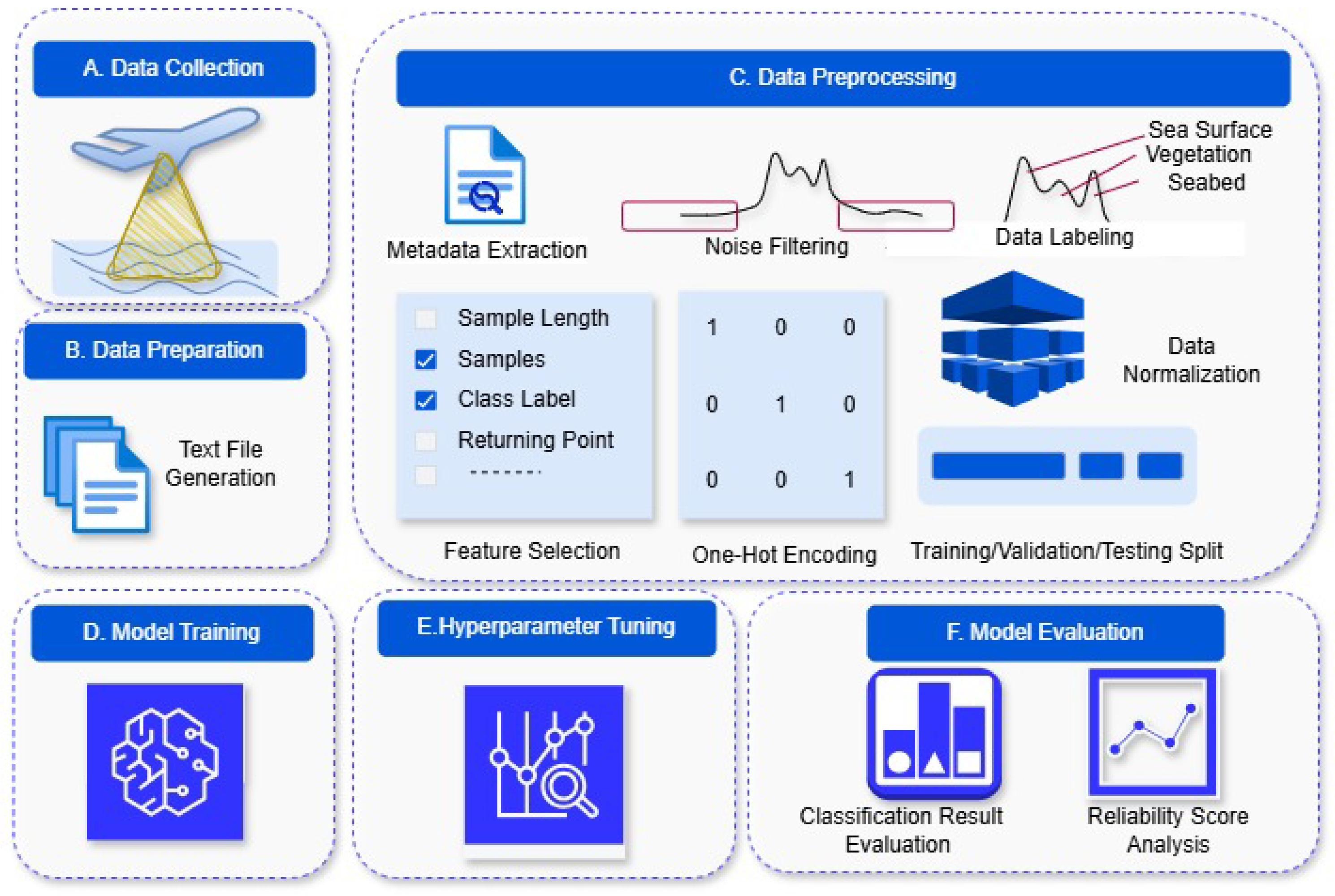
Figure 2.
Data collection Location: Fjøløy Island in Stavanger, Norway.
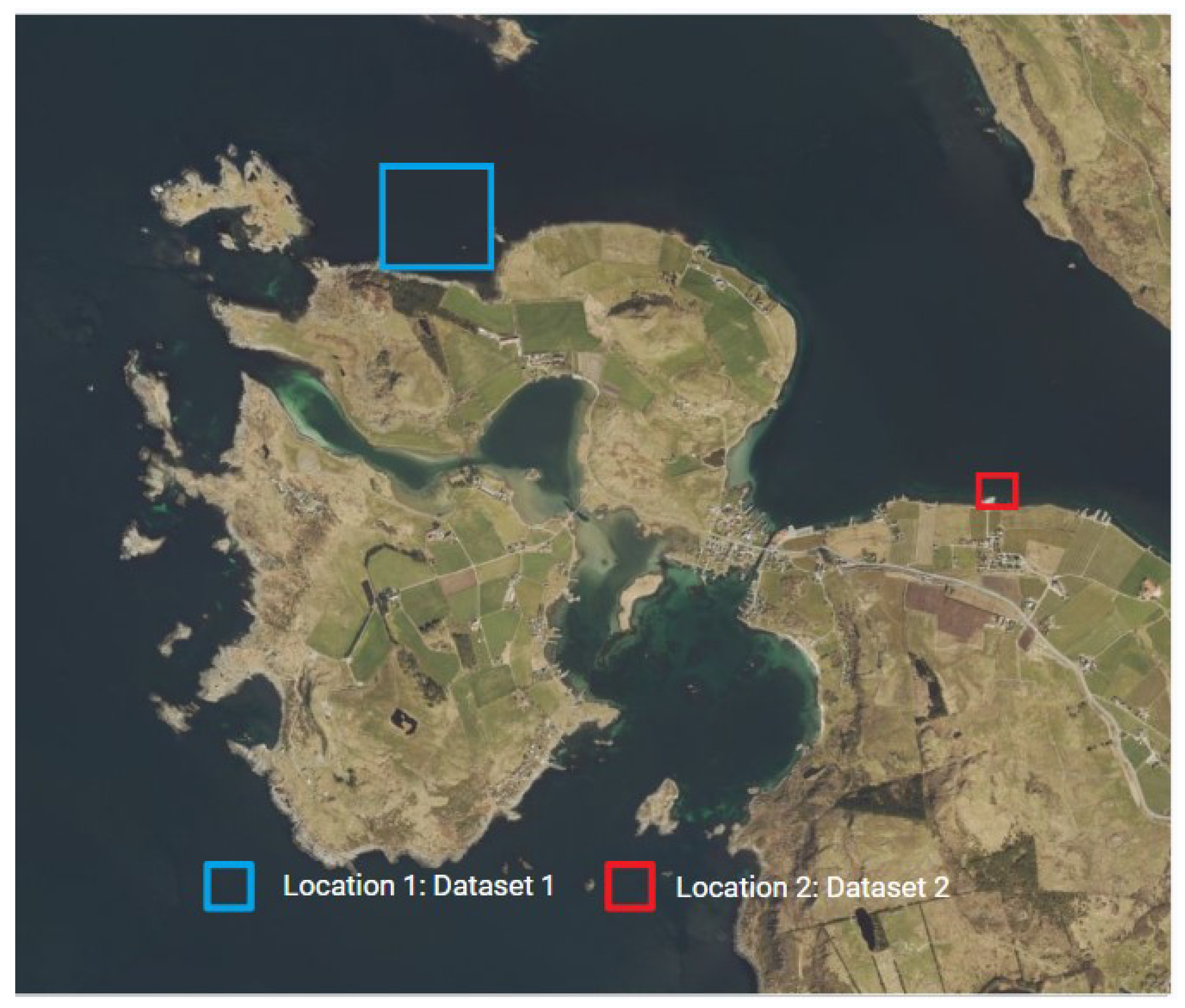
Figure 3.
Preview of a text file from Dataset 1.
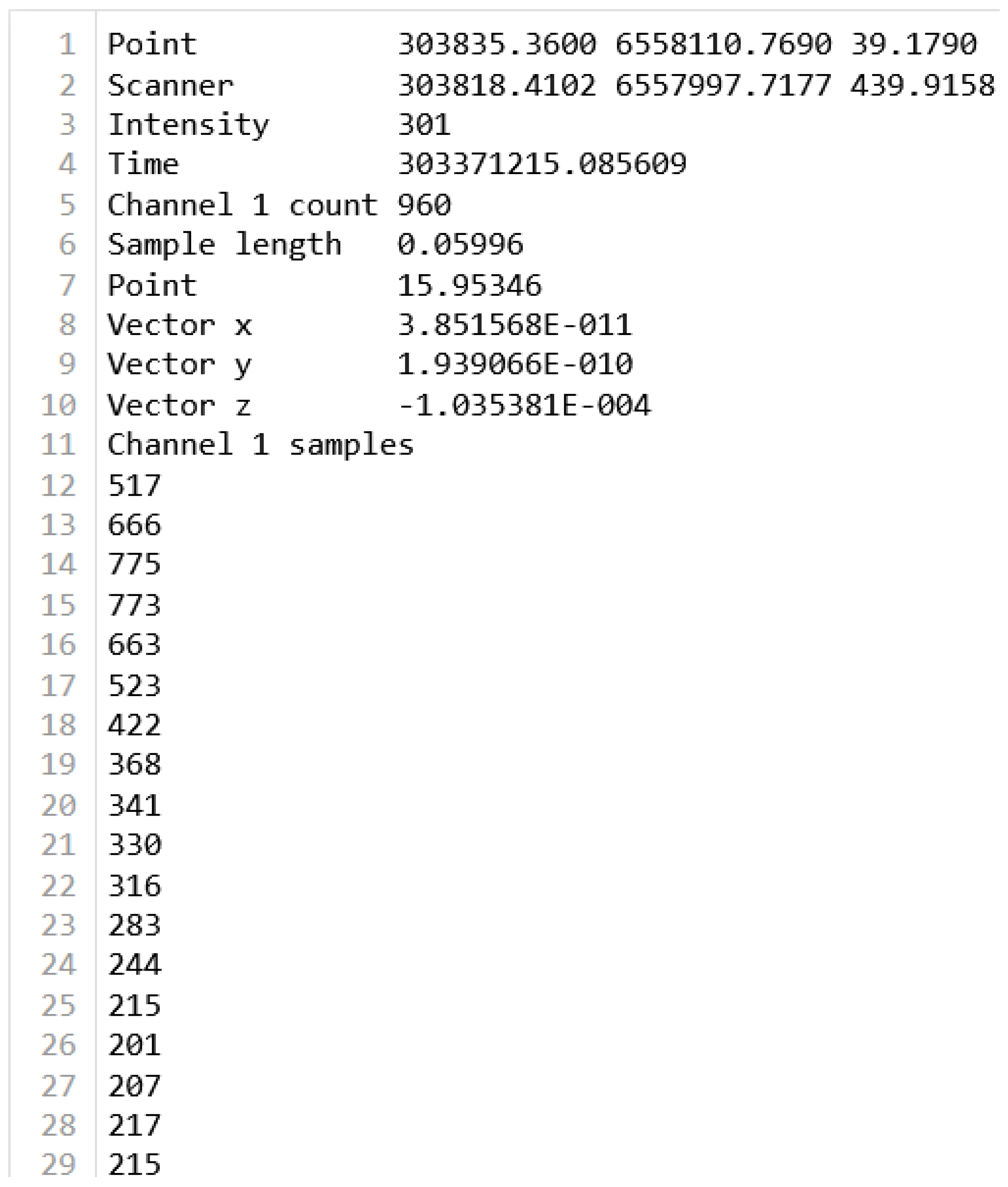
Figure 4.
Marked Peaks in a waveform.
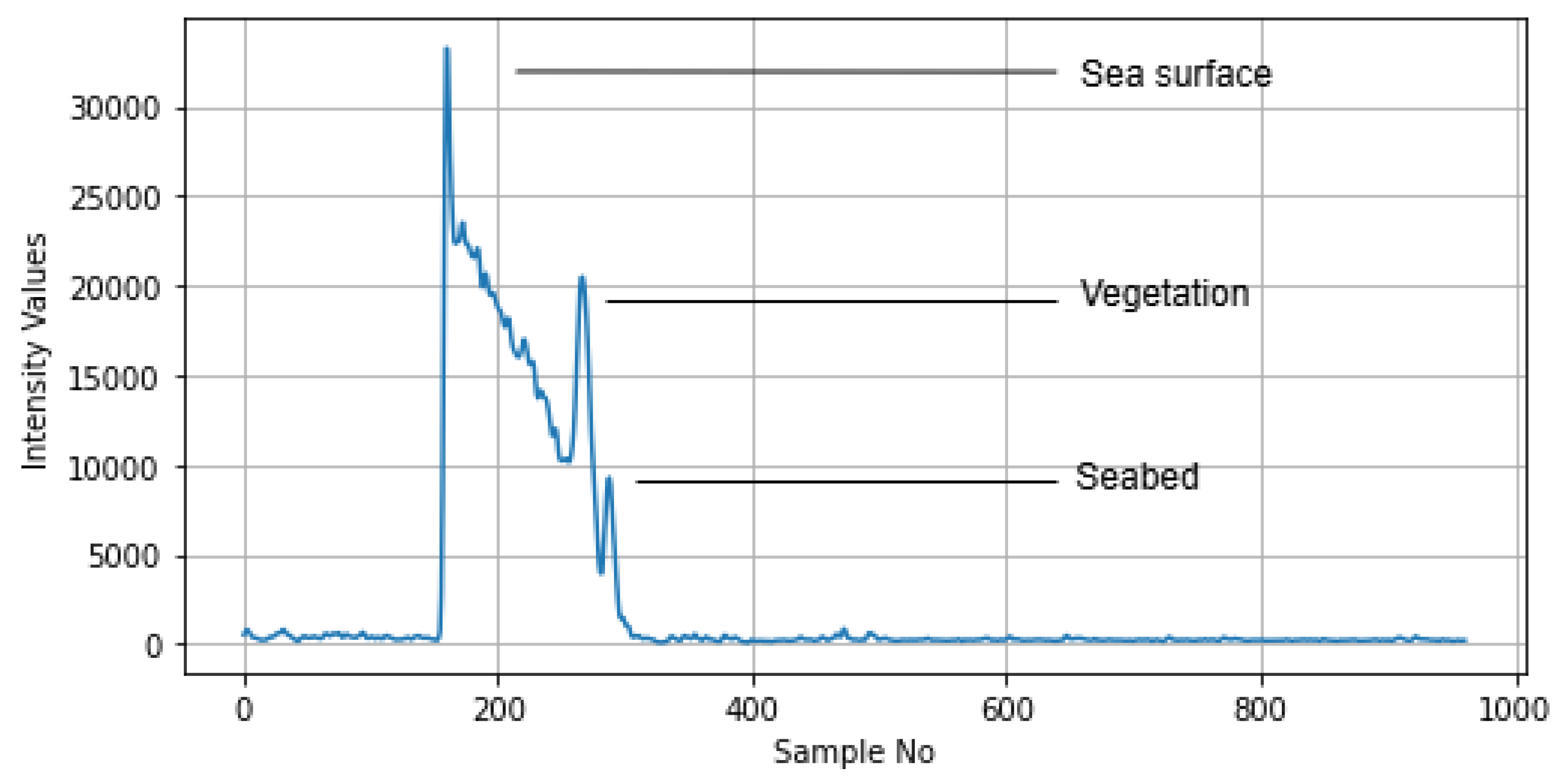
Figure 5.
Noise Filtering: The Intensity Values at the beginning (Sample_no 1-100) and at the end (Sample_no 401-960) are marked as Noise (see marked red lines).
Figure 5.
Noise Filtering: The Intensity Values at the beginning (Sample_no 1-100) and at the end (Sample_no 401-960) are marked as Noise (see marked red lines).
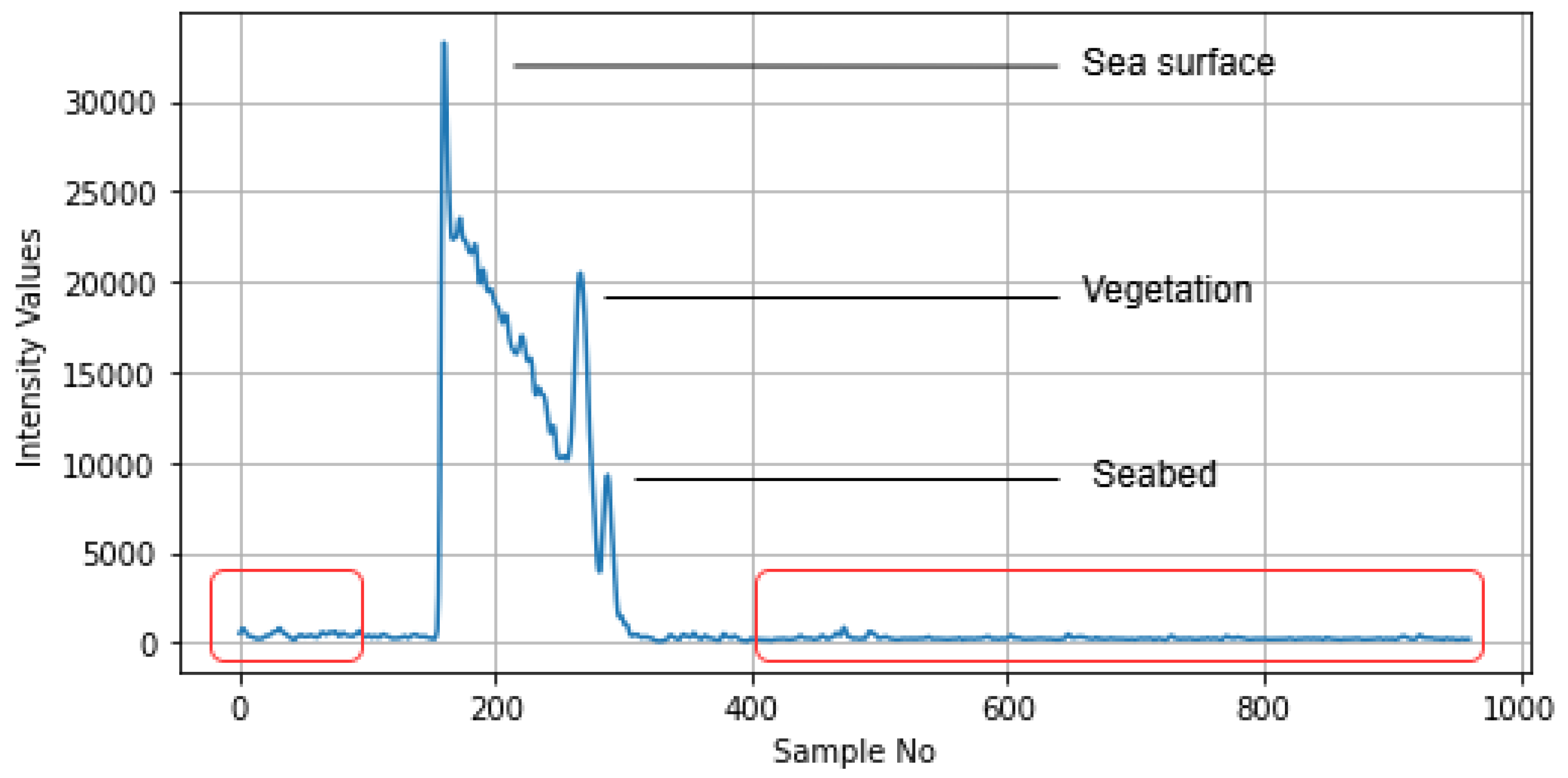
Figure 7.
Labeled classes.
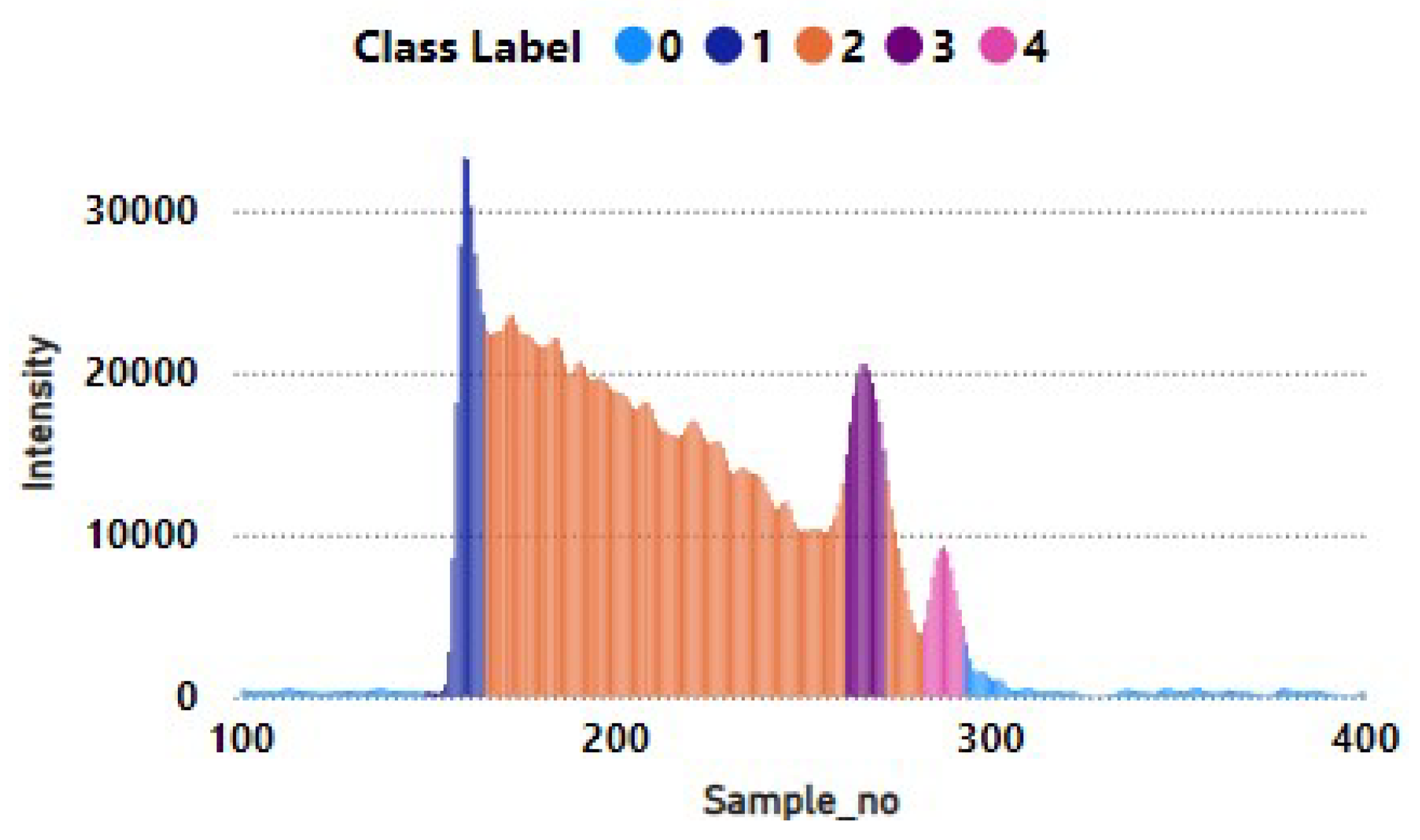
Figure 8.
Examples of labeled ALB waveforms showing detected peaks and class regions (sea surface, vegetation, and seabed).
Figure 8.
Examples of labeled ALB waveforms showing detected peaks and class regions (sea surface, vegetation, and seabed).
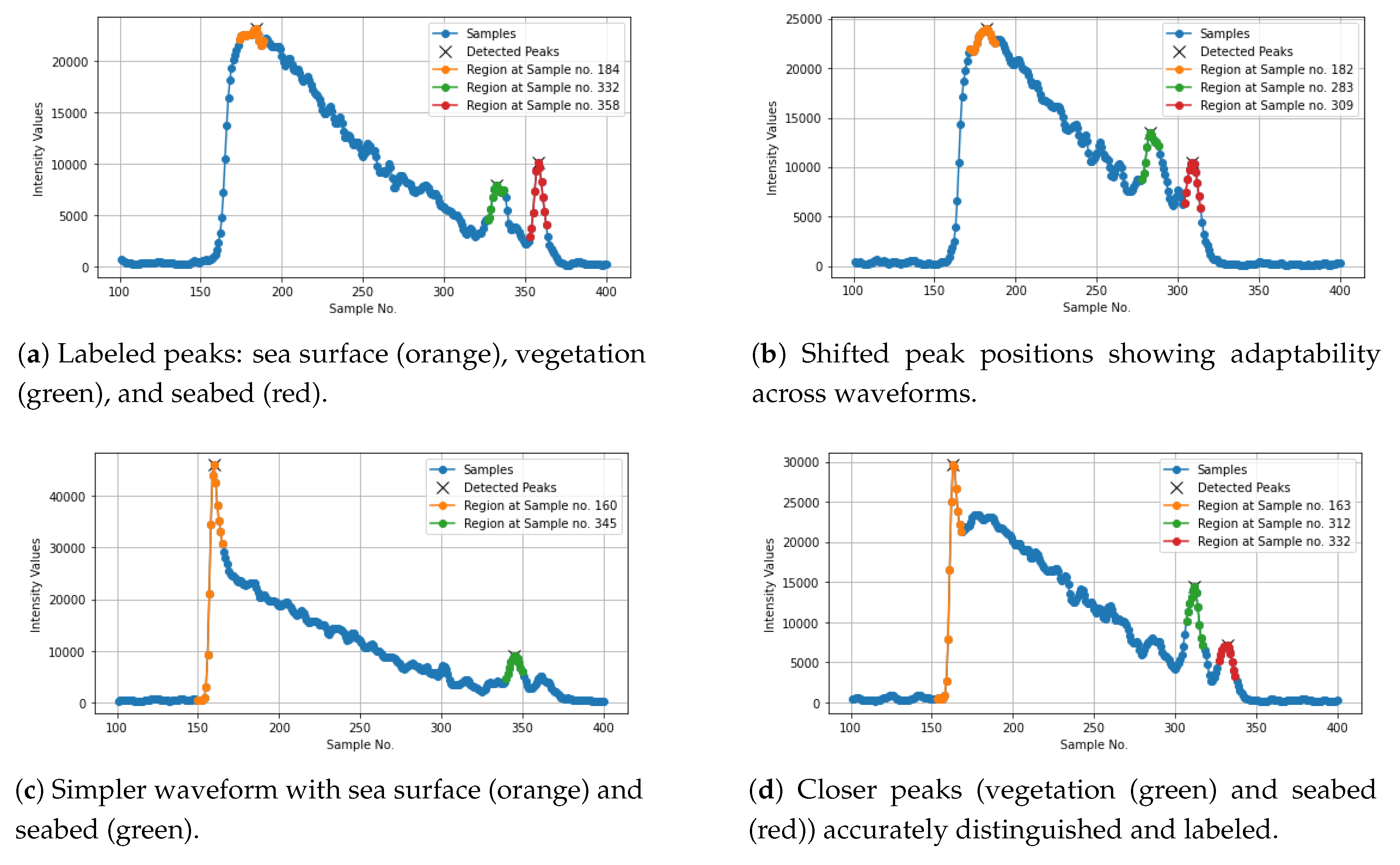
Figure 9.
The employed LSTM and BiLSTM Architectures.
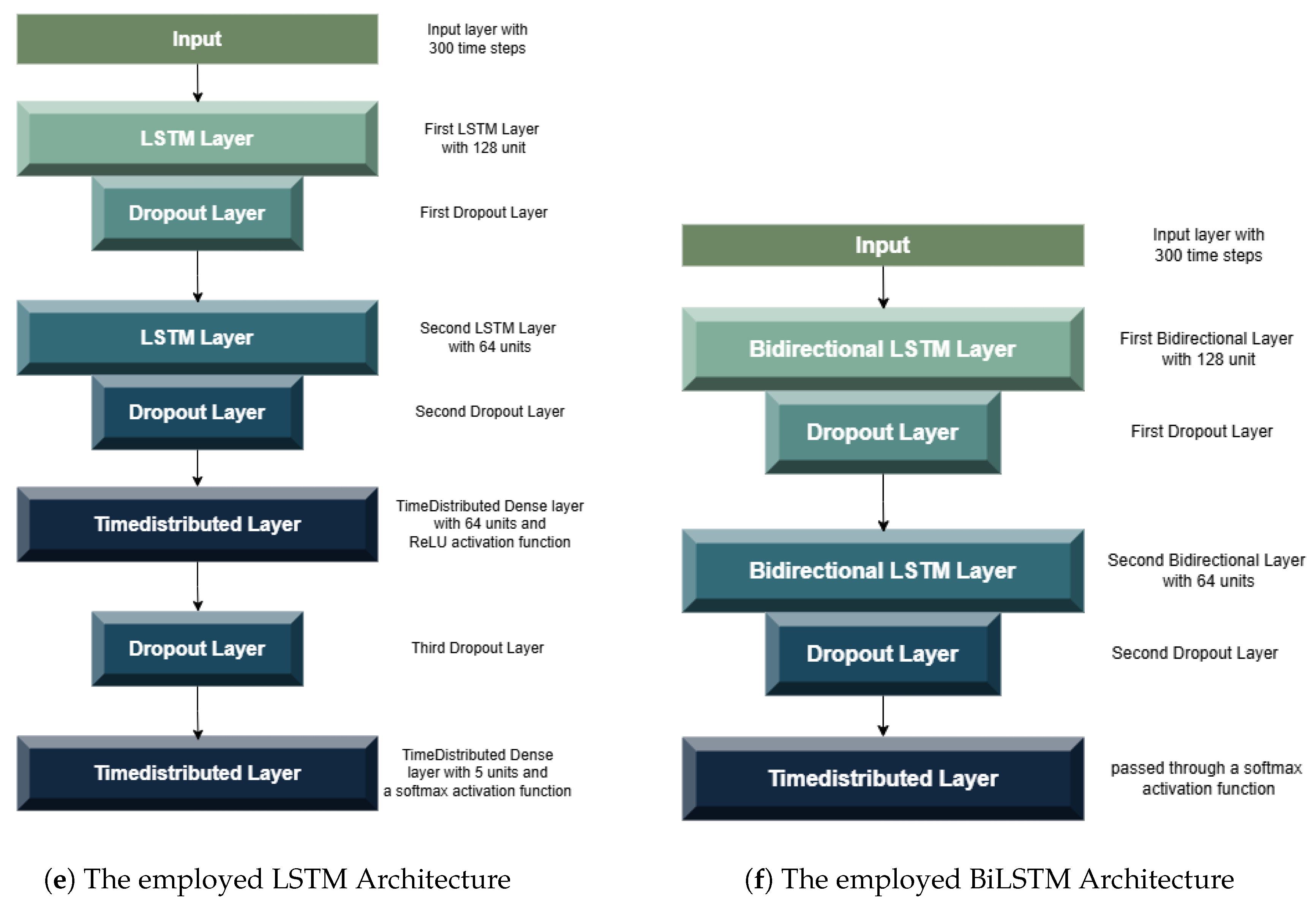

Table 1.
A Comparison of Our Work with the Existing Literature, modified from [17].
Table 1.
A Comparison of Our Work with the Existing Literature, modified from [17].
| Citations | Objective | Dataset/Location | Algorithm(s) | Obtained Results |
|---|---|---|---|---|
| [19] | Classification and detection of objects on the seabed |
The artificial reef Rosenort on the Baltic Sea. |
MLP | Accuracy: 92.07% |
| [20] | Improve seabed modeling and object detection |
The artificial reef Rosenort on the Baltic Sea. |
MLP | Accuracy: 97.0%, with LVQ SMOTE, 96%, with ROSE |
| [21] | Semantic segmentation of water surface and seabed |
Coastal-urban scenes of Tampa Bay, Florida, USA, |
SPG | Accuracy: 72.45% |
| [22] | Ocean–land waveform classification | Qinshan Island of Lianyungang City, Jiangsu Province, China |
MVCNN | Accuracy: 99.41% |
| [9] | Propose a deep learning frame work for nearshore bathymetry (DL-NB) |
Appalachian Bay (AB), Virgin Islands (VI), and Cat Island (CI) of the United States. |
2D CNN | RMSE was 1.01 m, 1.80 m and 0.28 m in AB, VI, and CI respectively |
| [23] | The classification of airborne laser bathymetry data to three classes (1) water surface, (2) seabed and (3) objects/obstacles. |
The artificial reef Rosenort on the Baltic Sea. |
RF | Accuracy: 100% water surface, 99.9% seabed and 60% objects. |
| [24] | Classify riverine land cover | Asahi River, Japan | Transfer Learning | Accuracy: 95% |
| [10] | Classification and mapping of the seafloor |
Polish coast, The Southern Baltic | KNN, SVM, RF |
Accuracy: varies from 75% to 91% |
| [25] | Bottom return residual analysis | The western Gulf of Maine, USA | SVM | Accuracy: 96% (sand and rock ) 86% (fine and coarse sand) |
| Our Work | Multi-class classification of underwater elements (Sea surface, Vegetation, Seabed, Water, Noise) |
Fjøløy island in Stavanger, Norway |
LSTM | Accuracy: Dataset 1: 95.22% Dataset 2: 94.85% |
| BiLSTM | Accuracy: Dataset 1: 94.37% Dataset 2: 84.18% |
Table 2.
Class Distribution among Two Datasets.
| Class | Class Name | Dataset 1 | Dataset 2 |
|---|---|---|---|
| 0 | Noise | 1,072,781 | 754,099 |
| 1 | Sea surface | 101,809 | 70,848 |
| 2 | Water | 615,134 | 450,087 |
| 3 | Vegetation | 53,863 | 4,658 |
| 4 | Seabed | 70,113 | 48,708 |
Table 3.
Computed Weights for the BiLSTM Model.
| Class_Label | Computed Weights | |
|---|---|---|
| Dataset 1 | Dateset 2 | |
| 0 | 0.3566 | 0.3522 |
| 1 | 3.7582 | 3.75 |
| 2 | 0.6225 | 0.5905 |
| 3 | 7.1032 | 56.7325 |
| 4 | 5.4594 | 5.4545 |
Table 4.
LSTM and BiLSTM Models’ Hyperparameter Tuning Setup.
| Feature | LSTM Model | BiLSTM Model |
|---|---|---|
| Model Type | Sequential LSTM | Bidirectional LSTM (BiLSTM) |
| Input Shape | (300, 1) | (300, 1) |
| First LSTM Layer | LSTM (128 units, return_sequences=True) | Bidirectional LSTM (128 units, return_sequences=True) |
| First Dropout Layer | Dropout (0.5) | Dropout (0.5) |
| Second LSTM Layer | LSTM (64 units, return_sequences=True) | Bidirectional LSTM (64 units, return_sequences=True) |
| Second Dropout Layer | Dropout (0.5) | Dropout (0.5) |
| Additional Layer | TimeDistributed Dense (64 units, ReLU activation) | N/A |
| Third Dropout Layer | Dropout (0.5) | N/A |
| Output Layer | TimeDistributed Dense (5 units, softmax) | TimeDistributed Dense (5 units, softmax) |
| Optimizer | Adam | Adam |
| Learning Rate | 1.00E-03 | 1.00E-04 |
| Loss Function | Categorical cross-entropy | Categorical cross-entropy |
| Metrics | Accuracy | Accuracy |
| Batch Size | 32 | 16 |
| Epochs | 100 | 100 |
| class Imbalance Handling | N/A | Sample weights used based on computed class weights |
Table 5.
The obtained results on both datasets.
| Dataset 1 | Dataset 2 | ||||
|---|---|---|---|---|---|
| LSTM | BiLSTM | LSTM | BiLSTM | ||
| Accuracy | 95.22% | 94.37% | 94.85% | 84.18% | |
| Macro Average | Precision | 0.8787 | 0.8039 | 0.7011 | 0.6112 |
| Recall | 0.8594 | 0.9486 | 0.6885 | 0.8359 | |
| F1-Score | 0.8641 | 0.8616 | 0.6945 | 0.635 | |
| Weighted Average | Precision | 0.9533 | 0.9587 | 0.9446 | 0.9482 |
| Recall | 0.9522 | 0.9437 | 0.9485 | 0.8418 | |
| F1-Score | 0.9518 | 0.9478 | 0.9464 | 0.8787 | |
Disclaimer/Publisher’s Note: The statements, opinions and data contained in all publications are solely those of the individual author(s) and contributor(s) and not of MDPI and/or the editor(s). MDPI and/or the editor(s) disclaim responsibility for any injury to people or property resulting from any ideas, methods, instructions or products referred to in the content. |
© 2025 by the authors. Licensee MDPI, Basel, Switzerland. This article is an open access article distributed under the terms and conditions of the Creative Commons Attribution (CC BY) license (https://creativecommons.org/licenses/by/4.0/).
Copyright: This open access article is published under a Creative Commons CC BY 4.0 license, which permit the free download, distribution, and reuse, provided that the author and preprint are cited in any reuse.


