
Submitted:
21 August 2025
Posted:
21 August 2025
You are already at the latest version
Abstract
The aim of the present paper is to develop further a theory on the flow of linguistic variables making a sentence, namely, the transformation: (a) characters into words; (b) words into word intervals; (c) word intervals into sentences. The relationship between two linguistic variables is studied as a communication channel whose performance is determined by the slope of their regression line and by their correlation coefficient. The theory is applicable to any field/specialty in which a linear relationship holds between two variables. The signal–to–noise ratio Γ is a figure of merit of a channel being deterministic, i.e. a channel in which the scattering of the data around the regression line is negligible. The larger Γ is, the more the channel is deterministic. In conclusion, humans have invented codes whose sequences of symbols making words cannot vary very much for indicating single physical or mental objects of their experience (larger Γ). On the contrary, a large variability (smaller Γ) is achieved by introducing interpunctions to make word intervals, and word intervals to make sentences to communicate concepts.
Keywords:
Balto−Slavic languages
; communication channels
; language processing
; Germanic languages
; Greek
; Latin
; New Testament
; Romance languages
; short−term memory
; translation
; Uralic languages
1. Introducing an Equivalent Input–Output Model of the Short–Term Memory
Humans can communicate and extract meaning both from spoken and written language. Whereas the sensory processing pathways for listening and reading are distinct, listeners and readers appear to extract very similar information about the meaning of a narrative story – heard or read – because the brain assimilates a written text like the corresponding spoken/heard text [1]. In the following, therefore, we consider the processing of reading or writing a text – a writer is also a reader of his/her own text – due to the same brain activity. In other words, the human brain represents semantic information in a modal form, independently of input modality.
How the human brain analyzes the parts of a sentence (parsing) and describes their syntactic roles is still a major question in cognitive neuroscience. In References [2,3], we proposed that a sentence is elaborated by the short–term memory (STM) with two independent processing units in series (equivalent surface processors), with similar size. The clues for conjecturing this input–output model emerged by considering many novels belonging to the Italian and English literatures. In Reference [3], we showed that there are no significant mathematical/statistical differences between the two literary corpora, according to the so–called surface deep–language parameters, suitably defined.
The model conjectures that the mathematical structure of alphabetical languages – digital codes created by the human mind for communication – seems to be deeply rooted in humans, independently of the particular language used or historical epoch. The complex and inaccessible mental process lying beneath communication – still largely unknown – can be studied by looking at the input–output functioning revealed by the structure of alphabetical languages.
The first processor is linked to the number of words between two contiguous interpunctions, variable indicated by – termed word interval (Appendix A lists the mathematical symbols used in the present article) – approximately ranging in Miller’s law range [4,5,6,7,8,9,10,11,12,13,14,15,16,17,18,19,20,21,22,23,24,25,26,27,28,29,30]. The second processor is linked to the number of’s contained in a sentence, referred to as the extended short–term memory (E–STM), ranging approximately from 1 to 6. These two units can process sentences containing approximately a number of words from to, values that can be converted into time by assuming a reading speed. This conversion gives seconds for a fast–reading reader [14], and seconds for a reader of novels, values well supported by experiments [15,16,17,18,19,20,21,22,23,24,25,26,27,28,29,30].
The E–STM must not be confused with the intermediate memory [31,32]. It is not modelled by studying neuronal activity, but by studying only the surface aspects of human communication due, of course, to neuronal activity, such as words and interpunctions, whose effects writers and readers experience since the invention of writing. In other words, the model proposed in References [2,3] describes the “input–output” characteristics of the STM. In Reference [33], we further developed the theory by including an equivalent first processor that memorizes syllables and characters to produce a word.
In conclusion, in References [2,3,33] we have proposed an input–output model of the STM, made of three equivalent linear processors in series, which independently process: (1) syllables and characters to make a word, (2) words and interpunctions to make a word interval; (3) word intervals to make a sentence. This is a simple, but a useful approach because the multiple brain process regarding speech/texts is not yet fully understood but characters, words and interpunctions – these latter are needed to distinguish word intervals and sentences – can be easily studied [34,35,36].
In other words, the model conjectures that the mathematical structure of alphabetical languages is deeply rooted in humans, independently of the particular language used or historical epoch. The complex and inaccessible mental process lying beneath communication – still largely unknown – is revealed by looking at the input–output functioning built–in in alphabetical languages of any historical epoch.
The literature on the STM and its various aspects is immense and multidisciplinary – we have recalled above only few references – but nobody – as far as we know – has considered the connections we found and discussed in References [2,3,33]. Our modelling of the STM processing by three units in series is new.
A sentence conveys meaning, of course, therefore the theory we have developed might be one of the necessary starting points to arrive at the Information Theory that will finally include meaning.
Today, many scholars are trying to arrive at a “semantic communication” theory or “semantic information” theory, but the results are still, in our opinion, in their infancy [37,38,39,40,41,42,43,44,45]. These theories, as those concerning the STM, have not considered the main “ingredients” of our theory, namely the number of characters per word , and , parameters that anybody understands and can calculate in any alphabetical language [34,35,36], as a starting point for including meaning, still a very open issue.
Aim of the present paper is twofold: (a) to further develop the theory proposed in Reference [2,3,33], and (b) apply it to the flow of linguistic variables making a sentence. This “signal” flow is built–in in the model proposed in Reference [33], namely, the transformation of: (a) characters into words; (b) words into word intervals; (c) word intervals into sentences, according to Figure 1. Since the connection between these linguistic variables is described by regression lines [34,35,36], in the present article we analyze experimental scatterplots between these variables
The article is ideally divided in two parts. In the first part – from Section 2 to Section 4 – we recall and further develop the theory of linear channels [2,3,33]; in the second part – from Section 5 to Section 8 – we apply it to a significant database of literary texts.
The database of literary texts considered is a large set of the New Testament (NT) books, namely the Gospels according to Matthew, Mark, Luke, John, the Book of Acts, the Epistle to the Romans, and the Apocalypse – 155 chapters in total, according to the traditional subdivision of these texts. We have considered the original Greek texts and their translation to Latin and to 35 modern languages, texts partially studied in Reference [35]. Notice that in this paper, “translation” is indistinguishable from “language” because we deal only with one translation per language.
We consider the NT books and their modern translations for two reasons: (a) they tell the same story, therefore it is meaningful to compare the translations in different languages; (b) they use common words – not the words of scientific/academic disciplines – therefore, they can give some clues on how most humans communicate.
After this introductory section, Section 2 presents the theory of linear regression lines and associated communication channels; Section 3 presents the connection of single linear channels; Section 4 proposes and discusses the theory of series connection of single channels affected by noise; Section 5 reports an exploratory data analysis of the NT texts; Section 6 reports findings concerning single channels, Section 7 concerning series connection of channels and Section 8 concerning cross channels; finally Section 9 summarizes the main findings and indicates future studies.
2. Theory of Linear Regression Lines and Associated Communication Channels
In this section, we recall and further expand the general theory stochastic variables linearly connected, originally developed for linguistic channels [35,36] but applicable to any other field/specialty in which a linear relationship holds between two variables.
Let (independent variable) and (dependent variable) linked by the line:
Notice that Eq. (1) models a deterministic relationship through the slope and the intercept . Since in most scatterplots between linguistic variables , in the following we assume
However, notice that if , the theory can be fully applied by defining a new dependent variable .
In general, the relationship between and is not deterministic, i.e., given by Eq. (1), but stochastic (random). Eq. (1) models, in fact, two variables perfectly correlated – correlation coefficient – characterized by a multiplicative “bias” In general, however, these conditions do not hold, therefore Eq. (1) can be written as:
In Eq. (3) is an additive Gaussian stochastic variable with zero mean value [34,35,36], therefore Eq. (3) models a noisy linear channel. Notice that must not be confused with an intercept .
Figure 2 shows the flow chart describing Eq. (1) and Eq. (3) with a system/channel representation. The black box indicated with represents the deterministic channel, i.e. Eq. (1); the black box indicated with represents the parallel channel due to the scattering of around the regression line. The additive noise is a Gaussian stochastic variable with zero mean that makes the linear channel partially stochastic, namely “noisy”.
Now, let us consider:
- a)
- The variance of the difference between the values calculated with Eq. (1) and those calculated with (45° line) at given value, as the “regression noise” power [35]. This “noise” is due to the multiplicative bias between the two variables.
- b)
- The variance of the difference between the values not lying on Eq. (1) (), and those lying on it (), as the “correlation noise” power [35]. This “noise” is due to the spread of around the line given by Eq. (1), modelled by .
- c)
- Let and be the variances of and.
In case (a), we get the difference therefore the variance (or power) of the values lying on the regression line, regression noise, is given by:
Now, we define the regression noise−to−signal power ratio (NSR), as:
In case (b), the fraction of the variance due to the values of not lying on the regression line (correlation noise power,) is given by [46]:
The parameter is called the coefficient of determination and it is proportional to the variance of explained by the regression line [46]. However, this variance is correlated with the slope because the fraction of the variance due to the regression line, namely , is related to according to [46]:
Figure 3 shows the flow chart of variances.
Therefore, inserting Eq. (7) in Eq. (6), we get the correlation NSR, :
Now, since the two noise sources are disjoint, the total NSR of the channel shown in Figure 2, Figure 3 is given by:
Therefore, depends only on the two parameters and of the regression line:
Finally, the signal−to−noise ratio (SNR) is given by:
In decibel:
Of course, we expect that no channel can yield and , therefore . In empirical scatterplots, very likely, .
In conclusion, the slope measures the multiplicative “bias” of the dependent variable compared to the independent variable in the deterministic channel; the correlation coefficient measures how “precise” the linear best fit is.
Finally, notice the more direct and insightful analysis that can be achieved by using the NSR instead of the more common SNR because, in Eq. (9), the single channel NSRs simply add together. This makes easy to study, for example, which addend determines , and thus , while this is by far less easy with Eq. (11). Moreover, this choice leads also to a useful graphical representation of Eq. (10) that can guides analysis and design [11], as shown in Section 8.
In the next sections, we apply the theory of linear channel modeling to specific cases.
3. Connection of Single Linear Channels
We first study how the output variable of channel relates to the output variable of another similar channel for the same input . This channel is termed “cross channel” and it is fundamental in studying language translation [35]. Secondly, we study how the output of a deterministic channel, modelled by Eq. (1), relates to the output of its stochastic version, Eq. (3).
3.1. Cross Channels
Let us consider a scatterplot and a scatterplot in which the independent variable and the dependent variable are linked by linear regression lines:
As discussed in Section 2, Eqs. (13)(14) do not give the full relationship between the two variables because they link only conditional average values, measured by the slopes and in the deterministic channels. According to Eq. (3), we can write more general linear relationships by considering the scattering of the data, always present in experiments, modelled by additive Gaussian zero–mean noise sources and .
Now, we can develop a series of interesting investigations on these equations. By eliminating we can compare the dependent variable of Eq. (16) to the dependent variable of Eq. (15) for . In doing so, we can find the regression line and the correlation coefficient of the new scatterplot linking to without the availability of the scatterplot itself.
By eliminating between Eq.(15) and Eq. (16), we get:
Compared to the new independent variable , the slope of the regression line is given by:
Because the two Gaussian noise sources are independent and additive, the total noise is given by:
Figure 4 shows the flow chart describing the cross–channel.
Now, from Eq. (18), of the new channel is:
The unknown correlation coefficient between and is given by [35]:
Therefore, of the new channel is:
In conclusion, in the new channel connecting to we can determine the slope and the correlation coefficient of the scatterplot between and for the same value of the independent variable . Now, the availability of this scatterplot is experimentally very rare because it is unlikely to find values of and for exactly the same value of , therefore cross channels can reveal relationships very difficult to discover experimentally.
In the next sections, we further developed the theory of linear channels, originally established in Reference [35] for cross channels.
3.2. Stochastic Versus Deterministic Channel
We compare a deterministic channel with a stochastic channel derived from channel by adding noise. In other words, we start from the regression line given by Eq. (1) and then add noise due to the correlation coefficient . Therefore, from the theory of stochastic channels discussed in Section 3.1, we get:
In conclusion, in transforming a deterministic channel into a stochastic channel only the correlation noise is present, therefore the SNR is given by:
Eq. (29) coincides with the ratio between the variance explained by the regression line (proportional to the coefficient of determination ) and the variance due to the scattering (correlation noise), proportional to [46].
So far, we have considered single channels. In the next section, we consider the series connection of single channels to determine the SNR of the overall channel.
4. Series Connection of Single Channels Affected by Correlation Noise
In this section, we consider a channel made of series of single channels. We consider this case because it can be found in many specialties, and because in Section 7 we apply it to specific linguistic channels.
Figure 5 shows the flow chart of three single channels in series These channels can be characterized as done in Section 3.2, i.e., only with the correlation noise, therefore, the overall channel is compared to the deterministic channel in which:
From Figure 5, it is evident that the output noise of a preceding channel produces additive noise at the output of the next channel in series. The purpose of this section is to calculate at the output of the series of channels.
Theorem. The NSR of linear channels in series, each characterized by the correlation noise–to–signal ratio , is given by:
Proof. Let the three linear relationships of the isolated channels of Figure 5 (i.e., before connecting them in series) given by:
Let , , the variances (power) of the variables, and let , the variances (power) of the Gaussian zero–mean noise , , , then the NSRs of the isolated channels are given by:
When the first two blocks are connected in series, the input to the second block must include also the output noise of the first block, therefore from Eqs. (31)(33) we get the modified output variable :
In eq. (37), is the output “signal” and is the output noise, therefore, the NSR at the output of the second block is:
Now, for three channels in series, it is sufficient to consider given by Eq. (38) as the input NSR to the third single channel to obtain the final NSR and prove Eq.(30):
Finally, notice that of Eq. (30) is proportional to the mean :
In other words, the series channel averages the single.
In conclusion, Eqs. (30) – (40) allow studying channels made by the series of several single channels affected by correlation noise by simply adding their single NSRs.
In the next sections, we apply the theory to linguistic channels suitably defined, after exploring the database on the NT mentioned in Section 1.
5. Exploratory Data Analysis
In this second part, we explore the linear relationships between characters, words, interpunctions and sentences, according to the flow chart shown in Figure xx, of the New Testament books considered (Matthew, Mark, Luke, John, Acts, Epistle to the Romans, Apocalypse). This is the database of our experimental analysis and application of the theory of linear channels discussed in the previous sections.
Table 1 lists language of translation and language family, with total number of characters (, words (, sentences () and interpunctions ().
Figure 6 shows the scatterplots in the original Greek texts between: (a) characters and words; (b) words and interpunctions; (c) interpunctions and sentences; (d) characters and sentences. Figure 7 shows these scatterplots in the English translation. Appendix B shows example of scatterplots in other languages. Table 2 reports slope and correlation coefficient of the indicated scatterplots (155 samples for each scatterplot) for each translation, namely the input parameters of our theory on communication channels. The differences between languages are due to the large “domestication” of the original Greek texts discussed in Reference [47].
The four scatterplots define fundamental linear channels and they are connected with important linguistic parameters, previously studied [34,35,36], namely:
- a)
- The number of characters per word, , given by the ratio between characters (abscissa) and words (ordinate) in Figure 6(a).
- b)
- The number of words between two successive interpunctions, – called the word interval – given by the ratio between interpunctions (abscissa) and words (ordinate) in Figure 6(b).
- c)
- The number of word intervals in sentences, , given by the ratio between sentences (abscissa) and interpunctions (interpunctions) in Figure 6(c).
Figure 6(d) shows the scatterplot between characters and sentences, which will be discussed in Section 7.
In the next section, we study the cannels corresponding to these scatterplots.
Figure 8 shows the probability distributions of the correlation coefficient and the coefficient of determination , for the scatterplots: words versus characters (green line); interpunctions versus words (cyan); sentences versus interpunctions (magenta). The black line refers to the scatterplot sentences versus characters; the red line refers to the series channel considered in Section 7, which links characters to sentences.
On correlation coefficients – and consequently, on the coefficient of determination, which determines the SNR – we notice the following remarkable findings:
- a)
- In any language, the largest correlation coefficient is found in the scatterplot between characters and words. The communication digital codes invented by humans show remarkable strict relationships between digital symbols (characters) and their sequences (words) to indicate items of their experience, material or immaterial. Languages do not differ from each other very much being in the range (Armenian, Cebuano) and being, overall .
- b)
- The smallest correlation coefficient is found in the scatterplot between characters and sentences, overall . This relationship must be, of course, the most unpredictable and variable because the many digital symbols that make a sentence can create an extremely large number of combinations, each delivering a different concept.
- c)
- The correlation coefficient (and also the coefficient of determination decreases as characters combine to create words, as words combine to create word intervals and as word intervals combine to create sentences.
The path just mentioned in item c) describes an increasing creativity and variety of meaning, other than that of the deterministic channel.
The characters–to–words channel shows the smallest , therefore, this channel is the nearest to be purely deterministic. It does not tend to be typical of a particular text/writer but more of a language because a writer has very little freedom in using words of very different length [34], if we exclude specialized words belonging to scientific and academic disciplines.
On the contrary, the channels words–to–interpunctions and the interpunctions–to–sentences are less deterministic, a writer can exercise his/her creativity of expression more freely, therefore these channels depend more on writer/text than on language. Finally, the big “jump” from characters to sentences gives the greatest freedom.
In conclusion, humans have invented codes whose sequences of symbols making words cannot variate very much for indicating single physical or mental objects of their experience. To communicate concepts, on the contrary, a large variability can be achieved by introducing interpunctions to form word intervals and word intervals to form sentences, the final depositary of human basic concepts.
Figure 9 shows the probability distributions of the slope . The black line (only partially visible because it is superposed to the red line) refers to the scatterplot sentences versus characters; the red line refers to the series channel that connects sentences to characters, discussed in Section 7.
On slopes, we notice the following important findings:
- a)
- The slope of the scatterplot between interpunctions and sentences (magenta line) is the largest in any language– overall – and determines the number of word intervals, contained in a sentence in its deterministic channel.
- b)
- The slope of the scatterplot between interpunctions and words (cyan line) determines the length of the word interval, , in its deterministic channel.
- c)
- The slope of the scatterplot between words and characters (green line) determines the number of characters per word, , in its deterministic channel. As discussed below, this channel is the most “universal” channel because, from language to language varies little, compared to other linguistic variables.
- d)
As reiterated above, the slopes describe deterministic channels. As discussed in Section 6, a deterministic channel is not “deterministic” for what concerns the number of concepts, because the same number of sentences can communicate different meanings by just changing words and interpunctions. What is “deterministic” is the size of the ensemble.
In the next section, we model single linguistic channels, i.e. channels not yet connected in series from the linear relationships shown above.
6. Single Linguistic Channels
In this section, we apply the theory developed in Section 3.2 to the scatterplots of Section 5, therefore, to the following single channels:
- (a)
- Characters–to–Words.
- (b)
- Words–to–Interpunctions.
- (c)
- Interpunctions–to–Sentences.
These single channels are modelled like in Figure 2, Figure 3, they are affected only by the regression noise. is obtained from Eq. (29) and drawn in Figure 10. Table 3 reports mean and standard deviation of in each channel.
- a)
- Languages show different due to the large degree of domestication of the original Greek texts [47].
- b)
- decreases steadily in this order: characters–to–words, words–to–interpunctions, interpunctions–to–sentences. A decreasing says, relatively, how much a channel is less deterministic.
- c)
- Words–to–interpunction and interpunctions–to–sentences have close values, therefore they show similar deterministic channels.
- d)
- Most languages have greater than that in Greek. This agrees with the finding that in modern translations of the Greek texts domestication prevails over foreignization [47].
- e)
- Finally, we can consider as a figure of merit of a linguistic channel being deterministic: the larger is, the more the channel is deterministic.
Figure 11 shows histograms (37 samples) of for each channel. The probability density function of can be modelled with a Gaussian model (therefore, is a lognormal stochastic variable) with mean and standard deviation reported in Table 3. Figure 12 shows the probability functions of which show, again, differences and similarities of the channels.
In conclusion, the large of the characters–to–words channel, in any language, indicates that the transformation of characters into words is the most deterministic.
7. Series Connection of Linguistic Channels Affected by Correlation Noise
Let us connect the three single channels to obtain the series channel shown in Figure 5 and apply the theory of Section 4. We first show the results concerning the theory of series channel, and then we compare the single channel characters–to–sentences to that obtained with the series of single channels.
Figure 13(a) shows the single NSRs and the series NSRs in linear units for each language; Figure 13(b) shows the corresponding (dB), partially already reported in Figure 10. We can notice that in the sum indicated in Eq.(30), the NSR of the characters–to–words channel is negligible compared to the other two NSRs. For example, in English (language no. 10), therefore against . In general, so that the characters–to–words channel can be ignored, to a first approximation, because it is about of the other two addends in Eq. (30).
For the characters–to–words channel, Figure 14(a) shows the slope calculated from the scatterplot between characters and sentences (Table 2) and the slope given by Eq. (30). The agreement is excellent, in practice the two values coincide (correlation coefficient 0.9998). Figure 14(b) shows scatterplot between the correlation coefficient calculated from the scatterplot between characters and sentences (Table 2) and that calculated by solving Eq. (29) for after calculating from Eq. (39). In this case, the two values are poorly correlated (correlation coefficient 0.3929). Finally, notice the difference between the probability of calculated by solving Eq. (29) for – red line in Figure 12 – and that calculated from the available scatterplots and regression line (Table 2), black line. The smoother red curve models more accurately the relationship between characters and sentences than the available scatterplot shown in Figure 6(d), because is proportional to the mean value of the single channels, see Eq. (40).
In conclusion, calculated in a series channel linking two variables is more reliable than that calculated from a single channel/scatterplot between the two variables.
In the next section, we apply the theory of cross–channels of Section 3.1.
8. Cross Channels: Language Translations
In cross channels we study how the output variable of channel relates to the output variable of another similar channel for the same input , therefore we apply the theory of Section 3.1. In this new channel, we can determine the slope and the correlation coefficient of the scatterplot between and for the same value of the independent variable , therefore cross channels can reveal relationships more difficult to discover experimentally.
From the database of the NT texts and the scatterplots of Figure 6, we can study at least three cross channels:
- a)
- The words–to–words channel, by eliminating characters, therefore the number of words are compared for the same number of characters.
- b)
- The interpunctions–to–interpunctions channel, by eliminating words, therefore, the number of words intervals are compared for the same number of words.
- c)
- The sentences–to–sentences channel, by eliminating interpunctions, therefore, the number of sentences are compared for the same number of word intervals.
Now, since these channels connect one independent variable in one language to the same (dependent) variable in another language, they describe very important linguistic channels, namely translation channels and they can be studied from this particular perspective. Therefore, cross channels in alphabetical texts describe the mathematics/statistics of translation, as we first studied in Reference [35].
Figure 15 shows the slope and the correlation coefficient by assuming Greek as language , namely the reference language, for the three cross channels We can notice the following:
- a)
- For most languages, in any cross channel, therefore most modern languages tend to use more words – for the same number of characters –; more word intervals –for the same number of words – and more sentences – for the same number of word intervals – than Greek. In other words, the corresponding deterministic channel (the channel characterized a multiplicative slope) is significantly biased compared to the original Greek texts.
- b)
- The correlation coefficient is always very near unity. Therefore the scattering of the data around the regression line is similar in all the three cross channels.
Figure 16 shows the findings assuming English as reference language. In this case, we consider the “translation” from English into the other languages [35]. Clear differences are noticeable:
- a)
- Words–to–words channel: for most languages . The multiplicative bias is small, language tend to use the same number of words of English. This was not the case for Greek. The correlation coefficient is practically unity for all languages. In other words, modern language tend to use the same number of words English, for the same number of characters, therefore domestication of the alleged translation of English to the other languages is moderate, compared to Greek or Latin (see languages 1 and 2 in Figure 16(a)).
- b)
- Interpunctions–to–interpunctions channel: the multiplicative bias is strong, as in is Greek, therefore, the deterministic cross channels are different from language to language. The correlation coefficient is more scattered than in Figure 15, and different from language to language. Curiously, in the channel English–to–Greek, , no bias The correlation coefficient is similar to that of the sentences–to–sentences channel.
- c)
- Sentences–to–sentences: for most languages, is similar to that of the interpunctions–to–interpunctions channel.
Since similar diagrams can be shown when other modern languages are considered as the independent language – not shown for brevity – we can conclude that the translation from Greek to modern languages show a high degree of domestication, due especially to the multiplicative bias, namely to the deterministic channels not to the stochastic part of the channel. In conclusion, the translation from a modern language into another modern language is mainly done through deterministic channels. Therefore, the SNR is mainly determined by .
This conclusion is visually evident in the scatterplot between and shown in Figure 17, where a constant value of traces an arch of circle [34]. It is clear that , in other words, in the three cross channels, is dominated by , in agreement with what shown in Figure 15, Figure 16.
Finally, Figure 18 shows mean value and standard deviation of in the three channels, by assuming the language indicated in abscissa as independent language/translation.
Notice that, overall, the probability distribution of can be modelled as Gaussian with mean value and standard deviation reported in Table 4 (for its calculation see Appendix C). Notice that cross channels have larger than the series channels (Table 3), because “translation” between two modern languages use mostly deterministic channels.
Figure 19 shows, as example, the modelling of the words–to–words overall channel.
Now, we conjecture the characteristics of the three channels for an indistinct human being, by merging all values, as done with words in Figure 19.
Figure xx shows the Gaussian probability density functions and their probability distributions of the overall in the three channels calculated with the values of Table 4. These distributions refer, therefore, to channels in which all languages merge in a single digital code. In other words, we might consider these probability distributions as “universal”, typical of humans using plain text.
From Figure 18, Figure 19 and Figure 20 and Table 4, it clearly emerges the following “universal” characteristics.
- a)
- The words–to–words channel is distinguished from the other two channels, with larger . This channel is the most deterministic.
- b)
- The interpunctions–to–interpunctions and sentences–to–sentences channels are very similar both in mean value and standard deviation of , therefore indicating a similar freedom in creating variations with respect to their deterministic channels.
9. Summary and Conclusions
How the human brain analyzes the parts of a sentence (parsing) and describes their syntactic roles is still a major question in cognitive neuroscience. In References [2,3,33], we proposed that a sentence is elaborated by the short–term memory with three independent processing units in series: (1) syllables and characters to make a word, (2) words and interpunctions to make a word interval; (3) word intervals to make a sentence.
This approach is simple but useful, because the multiple processing of the brain regarding speech/text is not yet fully understood but characters, words and interpunctions – these latter needed to distinguish word intervals and sentences – can be easily studied in any alphabetical language and epoch. Our conjecture, therefore, is that we can find clues on the performance of the mind, at a high cognitive level, by studying the most abstract human invention, namely the alphabetical texts.
The aim of the present paper was to further develop and complete the theory proposed in Reference [2,3,33], and then apply it to the flow of linguistic variables making a sentence, namely, the transformation of: (a) characters into words; (b) words into word intervals; (c) word intervals into sentences. Since the connection between these linguistic variables is described by regression lines, we have analyzed experimental scatterplots between the variables.
In the first part of the article, we have recalled and further developed the theory of linear channels, which models stochastic variables linearly connected. The theory is applicable to any field/specialty in which a linear relationship holds between two variables.
We have first studied how the output variable of channel relates to the output variable of another similar channel for the same input . These channels can be termed as “cross channels” and are fundamental in studying language translation.
Secondly, we have studied how the output of a deterministic channel relates to the output of its noisy version. A deterministic channel is not “deterministic” for what concerns the number of concepts, because, for example, the same number of sentences can communicate different meanings by just changing words and interpunctions. What is “deterministic” is the size of the ensemble.
Then, we have studied a channel made of series of single channels and have established that its noise–to–signal ratio is proportional to the average of the single channel noise–to–signal ratios.
In the second part of the article, we have explored, experimentally, the linear relationships between characters, words, interpunctions and sentences, in a large set of the New Testament books. We have considered the original Greek texts and their translation to Latin and to 35 modern languages because, in any language, they tell the same story, therefore it is meaningful to compare their translations. Moreover, they use common words, therefore, they can give some clues on how most humans communicate.
The characters–to–words channel is the nearest to be purely deterministic. It does not tend to be typical of a particular text/writer but more of a language because a writer has very little freedom in using words of very different length.
On the contrary, the channels words–to–interpunctions and the interpunctions–to–sentences are less deterministic, they depend more on writer/text than on language.
The signal–to–noise ratio is as a figure of merit of the deterministic channel. The larger is, the more the channel is deterministic.
In conclusion, humans have invented codes whose sequences of symbols making words cannot variate very much for indicating single physical or mental objects of their experience. On the contrary, to communicate concepts, a large variability is achieved by introducing interpunctions to make word intervals and word intervals to make sentences, the final depositary of human basic concepts. Future work should be devoted to non–alphabetical laguages.
Funding
This research received no external funding
Institutional Review Board Statement
Not applicable.
Informed Consent Statement
Not applicable
Data Availability Statement
Data are contained within the article.
Acknowledgments
Conflicts of Interest
The author declares no conflicts of interest.
Appendix A. List of mathematical symbols
| Symbol | Definition |
| Slope of regression line | |
| Slope in cross channel | |
| Correlation Coefficient in cross channel | |
| Number of characters per chapter | |
| Number of words per chapter | |
| Number of sentences per chapter | |
| Number of interpunctions per chapter | |
| Correlation coefficient of linear variables | |
| Coefficient of determination | |
| Standard deviation | |
| Variance | |
| Characters per word | |
| Word interval | |
| Word intervals per sentence | |
| Regression noise power | |
| Correlation noise power | |
| Regression noise−to−signal power ratio | |
| Correlation noise−to−signal power ratio | |
| Words per sentence | |
| Signal–to–noise ratio (linear) | |
| Signal–to–noise ratio (dB) | |
| Mean value |
Appendix B: Scatterplots in Different Languages
Figure A1.
Scatterplots in the French translation between: (a) characters and words; (b) words and interpunctions; (c) interpunctions and sentences; (d) between characters and sentences.
Figure A1.
Scatterplots in the French translation between: (a) characters and words; (b) words and interpunctions; (c) interpunctions and sentences; (d) between characters and sentences.
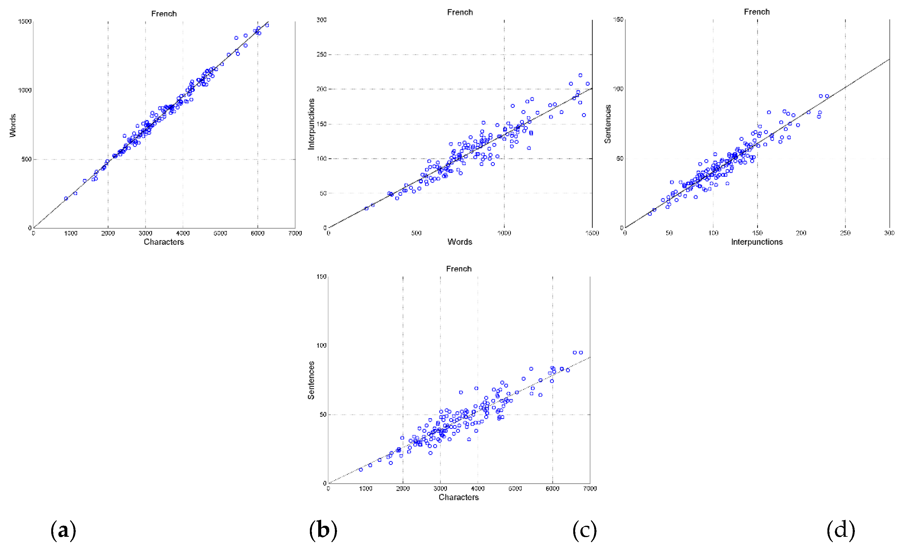
Figure A2.
Scatterplots in the Italian translation between: (a) characters and words; (b) words and interpunctions; (c) interpunctions and sentences; (d) between characters and sentences.
Figure A2.
Scatterplots in the Italian translation between: (a) characters and words; (b) words and interpunctions; (c) interpunctions and sentences; (d) between characters and sentences.
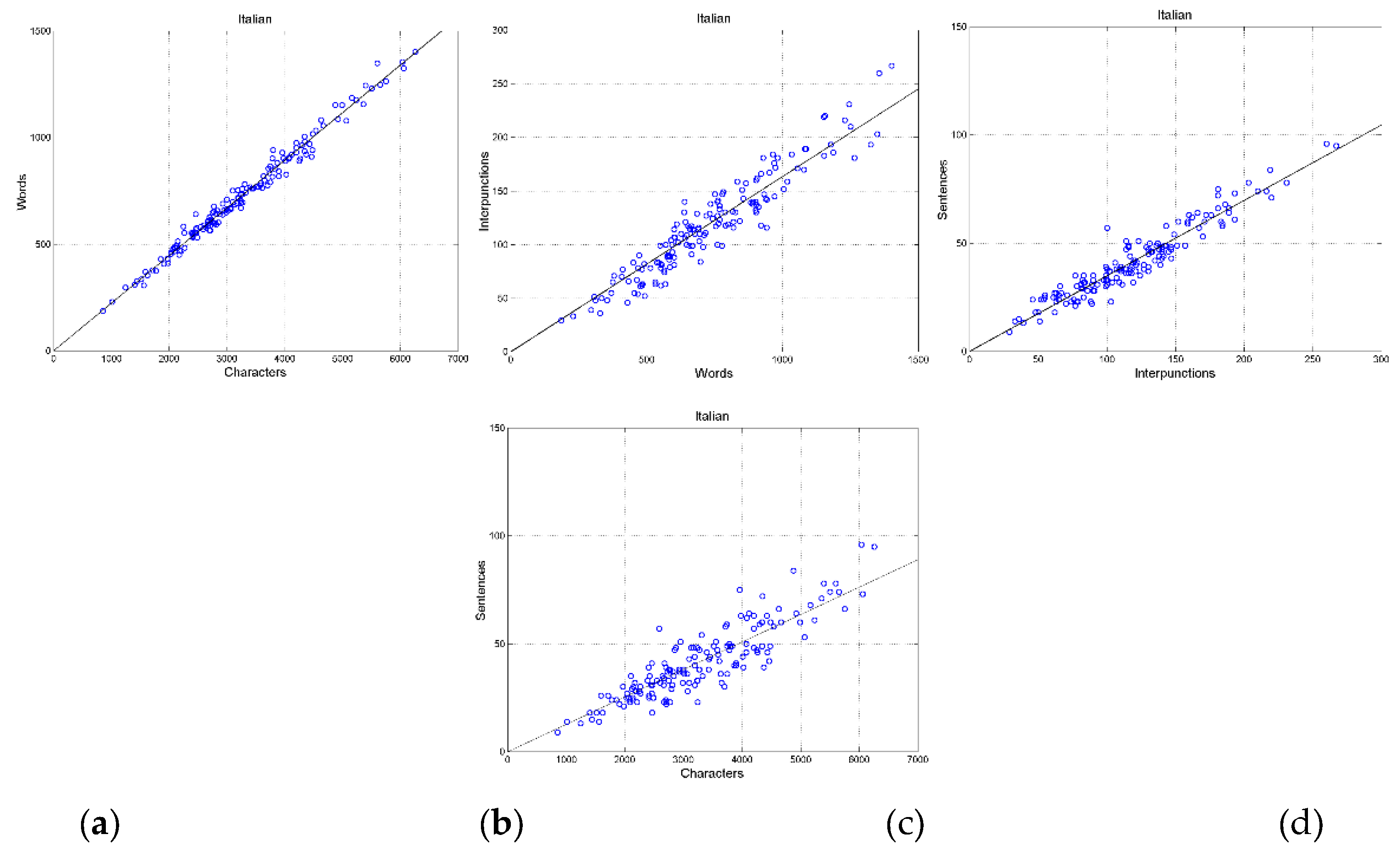
Figure A3.
Scatterplots in the Portuguese translation between: (a) characters and words; (b) words and interpunctions; (c) interpunctions and sentences; (d) between characters and sentences.
Figure A3.
Scatterplots in the Portuguese translation between: (a) characters and words; (b) words and interpunctions; (c) interpunctions and sentences; (d) between characters and sentences.
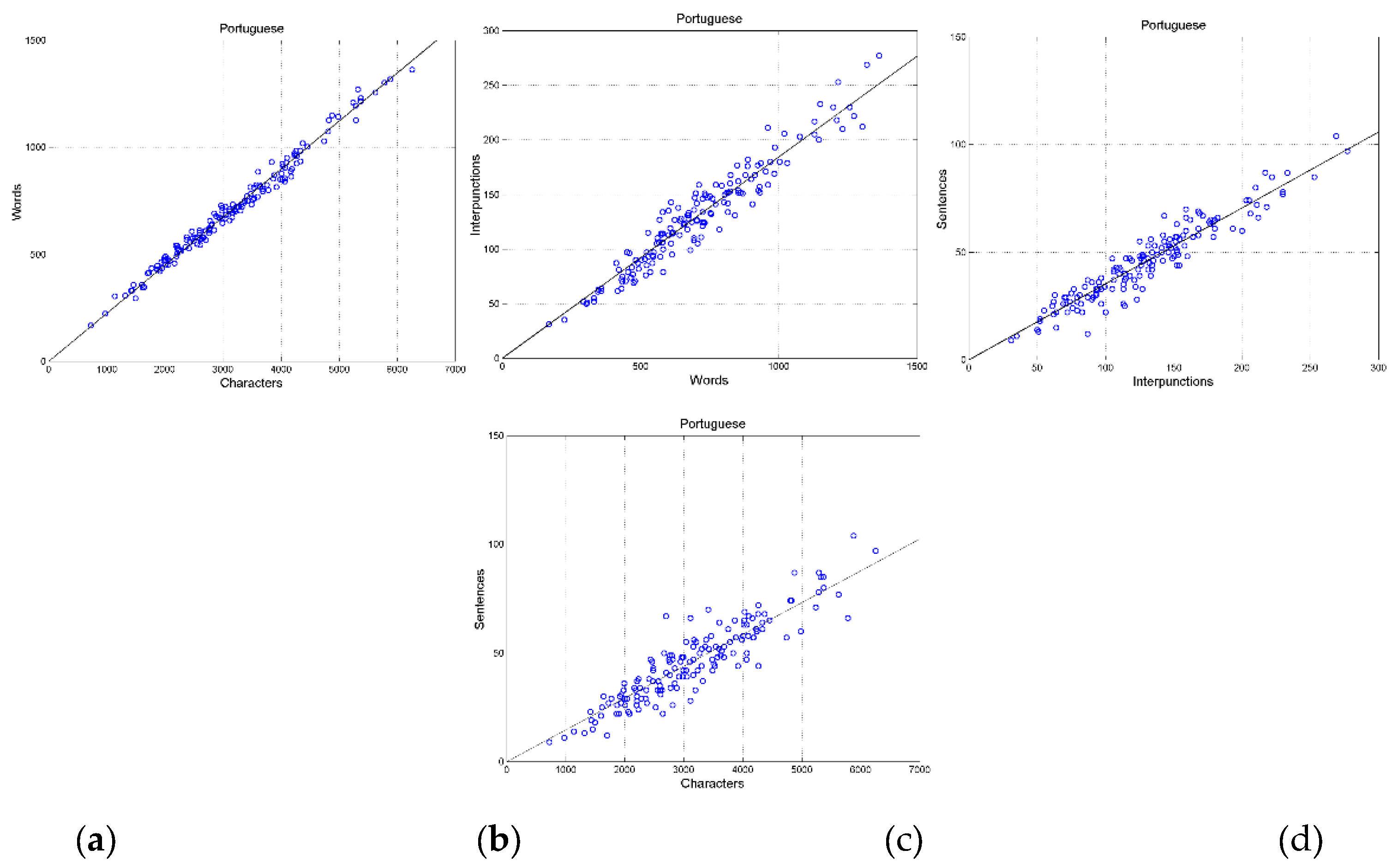
Figure A4.
Scatterplots in the Spanish translation between: (a) characters and words; (b) words and interpunctions; (c) interpunctions and sentences; (d) between characters and sentences.
Figure A4.
Scatterplots in the Spanish translation between: (a) characters and words; (b) words and interpunctions; (c) interpunctions and sentences; (d) between characters and sentences.
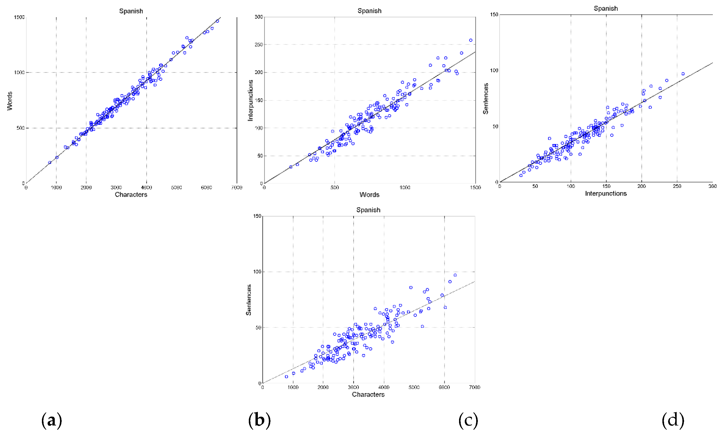
Figure A5.
Scatterplots in the German translation between: (a) characters and words; (b) words and interpunctions; (c) interpunctions and sentences; (d) between characters and sentences.
Figure A5.
Scatterplots in the German translation between: (a) characters and words; (b) words and interpunctions; (c) interpunctions and sentences; (d) between characters and sentences.
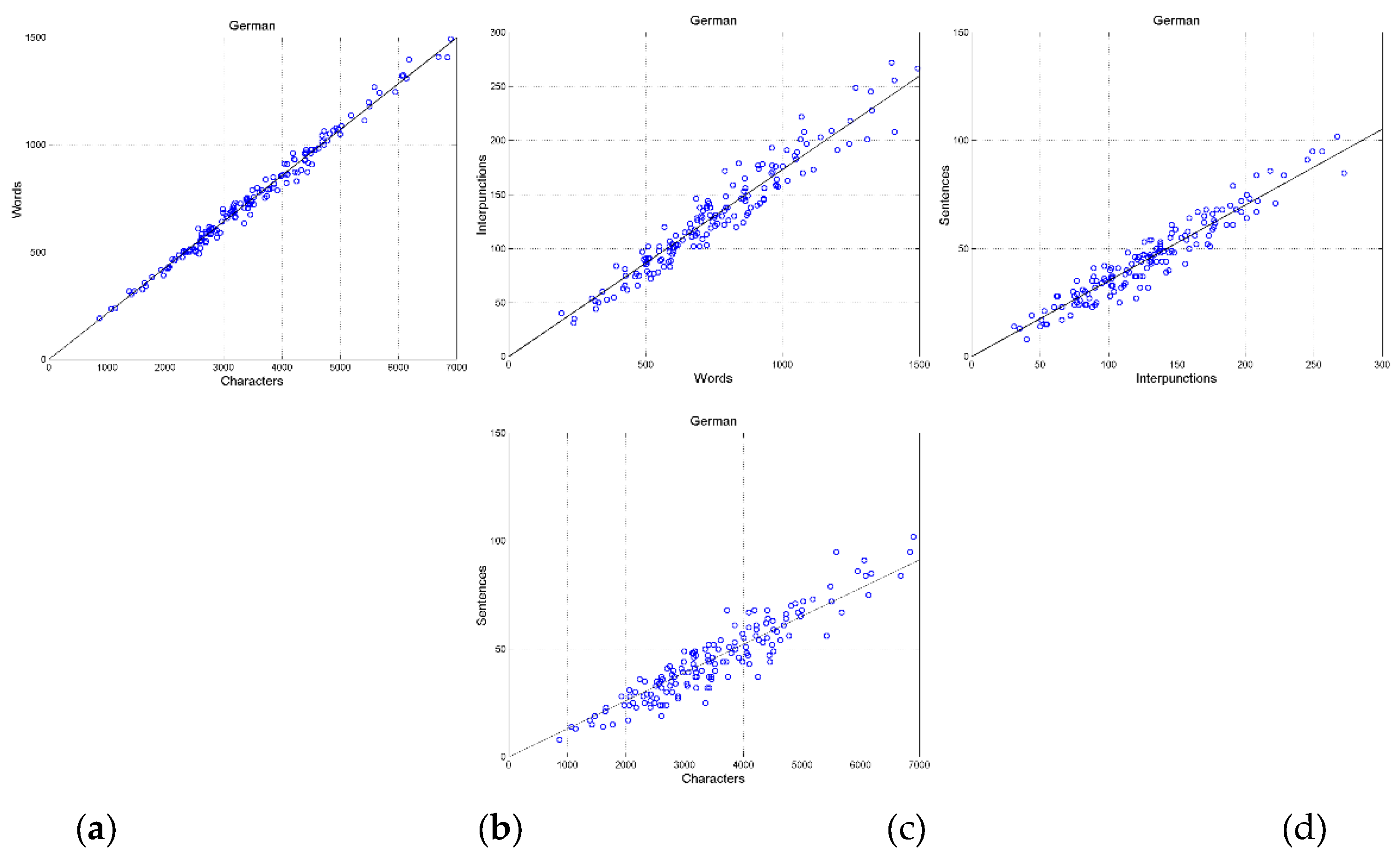
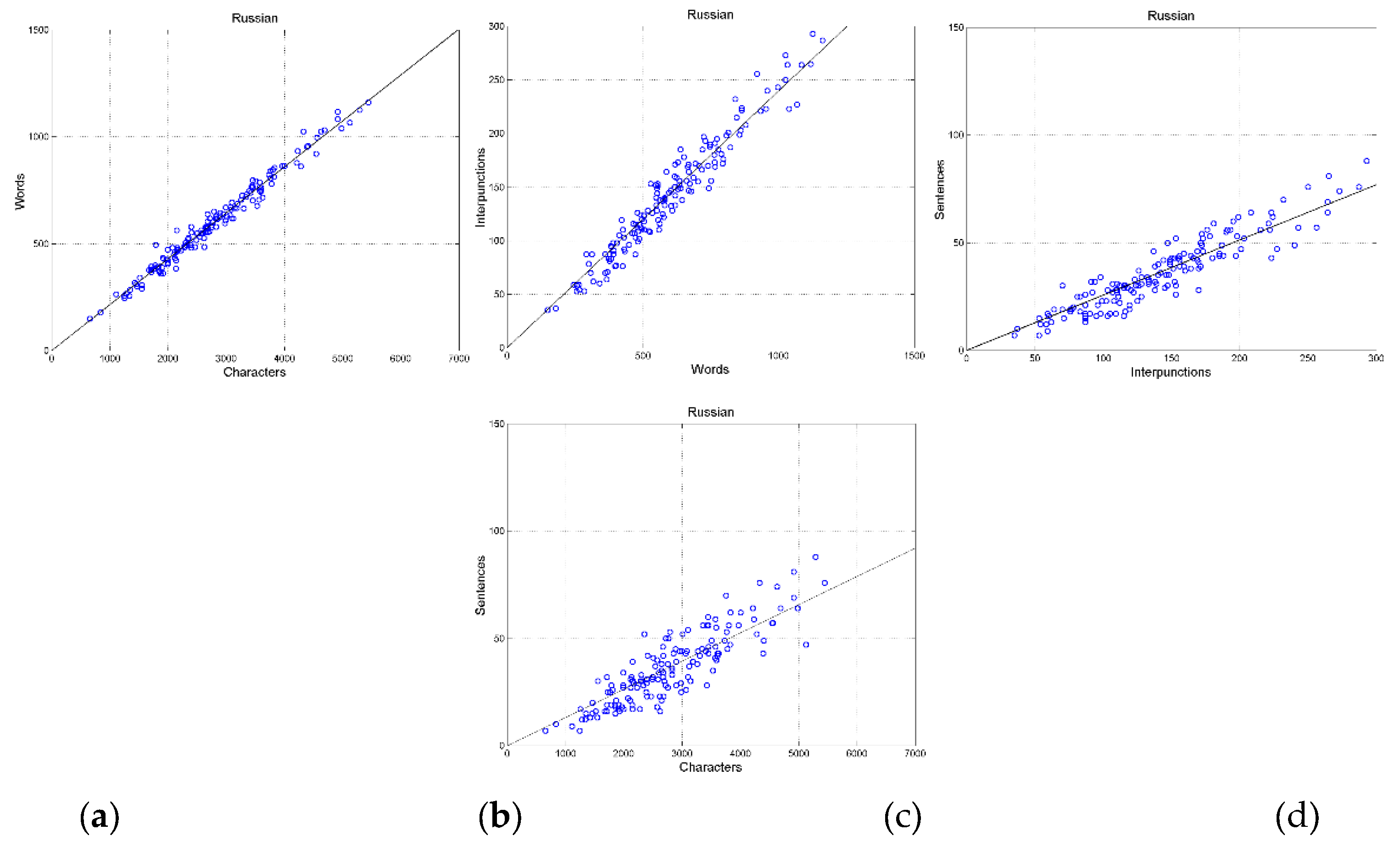
Figure A6.
Scatterplots in the Russian translation between: (a) characters and words; (b) words and interpunctions; (c) interpunctions and sentences; (d) between characters and sentences.
Figure A6.
Scatterplots in the Russian translation between: (a) characters and words; (b) words and interpunctions; (c) interpunctions and sentences; (d) between characters and sentences.
Appendix C
Let and be the (conditional) mean value and standard deviation of samples belonging to set , out of sets of the ensemble, e.g. the values shown in Figure xx. From statistical theory [86–88], the unconditional mean (ensemble mean) is given by the mean of means:
The unconditional variance (ensemble variance) ( is the unconditional standard deviation) is given:
From Eqs. (A1)–A(3), we get the overall values reported in Table 4.
References
- Deniz, F.; Nunez–Elizalde, A.O.; Huth, A.G.; Gallant Jack, L. The Representation of Semantic Information Across Human Cerebral Cortex During Listening Versus Reading Is Invariant to Stimulus Modality. J. Neuroscience 2019, 39, 7722–7736. [Google Scholar] [CrossRef]
- Matricciani, E. A Mathematical Structure Underlying Sentences and Its Connection with Short–Term Memory. AppliedMath 2024, 4, 120–142. [Google Scholar] [CrossRef]
- Matricciani, E. Is Short–Term Memory Made of Two Processing Units? Clues from Italian and English Literatures down Several Centuries. Information 2024, 15, 6. [Google Scholar] [CrossRef]
- Miller, G.A. The Magical Number Seven, Plus or Minus Two. Some Limits on Our Capacity for Processing Information. Psychological Review 1955, 343–352. [Google Scholar]
- Crowder, R.G. Short–term memory: Where do we stand? Memory & Cognition 1993, 21, 142–145. [Google Scholar] [CrossRef]
- Lisman, J.E.; Idiart, M.A.P. Storage of 7 ± 2 Short–Term Memories in Oscillatory Subcycles. Science 1995, 267, 1512–1515. [Google Scholar] [CrossRef] [PubMed]
- Cowan, N. ; The magical number 4 in short−term memory: A reconsideration of mental storage capacity. Behavioral and Brain Sciences 2000, 24, 87–114. [Google Scholar] [CrossRef]
- Bachelder, B.L. The Magical Number 7 ± 2: Span Theory on Capacity Limitations. Behavioral and Brain Sciences 2001, 24, 116–117. [Google Scholar] [CrossRef]
- Saaty, T.L.; Ozdemir, M.S. Why the Magic Number Seven Plus or Minus Two. Mathematical and Computer Modelling 2003, 38, 233–244. [Google Scholar] [CrossRef]
- Burgess, N.; Hitch, G.J. A revised model of short–term memory and long–term learning of verbal sequences. J. Mem. Lang. 2006, 55, 627–652. [Google Scholar] [CrossRef]
- Richardson, J.T.E. Measures of short–term memory: A historical review. Cortex 2007, 43, 635–650. [Google Scholar] [CrossRef] [PubMed]
- Mathy, F.; Feldman, J. What’s magic about magic numbers? Chunking and data compression in short−term memory. Cognition 2012, 122, 346–362. [Google Scholar] [CrossRef] [PubMed]
- Gignac, G.E. The Magical Numbers 7 and 4 Are Resistant to the Flynn Effect: No Evidence for Increases in Forward or Backward Recall across 85 Years of Data. Intelligence 2015, 48, 85–95. [Google Scholar] [CrossRef]
- Trauzettel−Klosinski, S.; Dietz, K. Standardized Assessment of Reading Performance: The New International Reading Speed Texts IreST. Investig. Opthalmology Vis. Sci. 2012, 53, 5452–5461. [Google Scholar] [CrossRef]
- Melton, A.W. Implications of Short–Term Memory for a General Theory of Memory. Journal of Verbal Learning and Verbal Behavior 1963, 2, 1–21. [Google Scholar] [CrossRef]
- Atkinson, R.C.; Shiffrin, R.M. The Control of Short–Term Memory. Scientific American 1971, 225, 82–91. [Google Scholar] [CrossRef]
- Murdock, B.B. Short–Term Memory. Psychology of Learning and Motivation 1972, 5, 67–127. [Google Scholar]
- Baddeley, A.D.; Thomson, N.; Buchanan, M. Word Length and the Structure of Short−Term Memory. Journal of Verbal Learning and Verbal Behavior 1975, 14, 575–589. [Google Scholar] [CrossRef]
- Case, R.; Midian Kurland, D.; Goldberg, J. Operational efficiency and the growth of short–term memory span. Journal of Experimental Child Psychology 1982, 33, 386–404. [Google Scholar] [CrossRef]
- Grondin, S. A temporal account of the limited processing capacity. Behavioral and Brain Sciences 2000, 24, 122–123. [Google Scholar] [CrossRef]
- Pothos, E.M.; Joula, P. Linguistic structure and short−term memory. Behavioral and Brain Sciences 2000, 138–139. [Google Scholar]
- Conway, A.R.A.; Cowan, N.; Michael, F.; Bunting, M.F.; Therriaulta, D.J.; Minkoff, S.R.B. A latent variable analysis of working memory capacity, short−term memory capacity, processing speed, and general fluid intelligence. Intelligence 2002, 30, 163–183. [Google Scholar] [CrossRef]
- Jonides, J.; Lewis, R.L.; Nee, D.E.; Lustig, C.A.; Berman, M.G.; Moore, K.S. The Mind and Brain of Short–Term Memory. Annual Review of Psychology 2008, 69, 193–224. [Google Scholar] [CrossRef]
- Barrouillest, P.; Camos, V. As Time Goes By: Temporal Constraints in Working Memory. Current Directions in Psychological Science 2012, 413–419. [Google Scholar] [CrossRef]
- Potter, M.C. Conceptual short–term memory in perception and thought. Frontiers in Psychology 2012. [Google Scholar] [CrossRef] [PubMed]
- Jones, G.; Macken, B. ; Questioning short−term memory and its measurements: Why digit span measures long−term associative learning. Cognition 2015, 1–13. [Google Scholar] [CrossRef] [PubMed]
- Chekaf, M.; Cowan, N.; Mathy, F. ; Chunk formation in immediate memory and how it relates to data compression. Cognition 2016, 155, 96–107. [Google Scholar] [CrossRef] [PubMed]
- Norris, D. Short–Term Memory and Long–Term Memory Are Still Different. Psychological Bulletin 2017, 143, 992–1009. [Google Scholar] [CrossRef]
- Houdt, G.V.; Mosquera, C.; Napoles, G. ; A review on the long short–term memory model. Artificial Intelligence Review 2020, 53, 5929–5955. [Google Scholar] [CrossRef]
- Islam, M.; Sarkar, A.; Hossain, M.; Ahmed, M.; Ferdous, A. Prediction of Attention and Short–Term Memory Loss by EEG Workload Estimation. Journal of Biosciences and Medicines 2023, 11, 304–318. [Google Scholar] [CrossRef]
- Rosenzweig, M.R.; Bennett, E.L.; Colombo, P.J.; Lee, P.D.W. Short–term, intermediate–term and Long–term memories. Behavioral Brain Research 1993, 57, 193–198. [Google Scholar] [CrossRef]
- Kaminski, J. Intermediate–Term Memory as a Bridge between Working and Long–Term Memory. The Journal of Neuroscience 2017, 37, 5045–5047. [Google Scholar] [CrossRef] [PubMed]
- Matricciani, E. Equivalent Processors Modelling the Short–Term Memory. Preprints 2025, 2025061906. [Google Scholar] [CrossRef]
- Matricciani, E. Deep Language Statistics of Italian throughout Seven Centuries of Literature and Empirical Connections with Miller’s 7 ∓ 2 Law and Short–Term Memory. Open Journal of Statistics 2019, 9, 373–406. [Google Scholar] [CrossRef]
- Matricciani, E. A Statistical Theory of Language Translation Based on Communication Theory. Open J. Stat. 2020, 10, 936–997. [Google Scholar] [CrossRef]
- Matricciani, E. Multiple Communication Channels in Literary Texts. Open Journal of Statistics 2022, 12, 486–520. [Google Scholar] [CrossRef]
- Strinati, E.C.; Barbarossa, S. 6G Networks: Beyond Shannon Towards Semantic and Goal–Oriented Communications. Computer Networks 2021, 190, 1–17. [Google Scholar] [CrossRef]
- Shi, G.; Xiao, Y.; Li, Y.; Xie, X. From semantic communication to semantic–aware networking: Model, architecture, and open problems. IEEE Communications Magazine 2021, 59, 44–50. [Google Scholar] [CrossRef]
- Xie, H.; Qin, Z.; Li, G.Y.; Juang, B.H. Deep learning enabled semantic communication systems. IEEE Trans. Signal Processing 2021, 69, 2663–2675. [Google Scholar] [CrossRef]
- Luo, X.; Chen, H.H.; Guo, Q. Semantic communications: Overview, open issues, and future research directions. IEEE Wireless Communications 2022, 29, 210–219. [Google Scholar] [CrossRef]
- Wanting, Y.; Hongyang, D.; Liew, Z.Q.; Lim, W.Y.B.; Xiong, Z.; Niyato, D.; Chi, X.; Shen, X.; Miao, C. Semantic Communications for Future Internet: Fundamentals, Applications, and Challenges. IEEE Communications Surveys & Tutorials 2023, 25, 213–250. [Google Scholar] [CrossRef]
- Xie, H.; Qin, Z.; Li, G.Y.; Juang, B.H. Deep learning enabled semantic communication systems. IEEE Trans. Signal Processing 2021, 69, 2663–2675. [Google Scholar] [CrossRef]
- Bellegarda, J.R. Exploiting Latent Semantic Information in Statistical Language Modeling. Proceedings of the IEEE 2000, 88, 1279–1296. [Google Scholar] [CrossRef]
- D’Alfonso, S. On Quantifying Semantic Information. Information 2011, 2, 61–101. [Google Scholar] [CrossRef]
- Zhong, Y. A Theory of Semantic Information. China Communications 2017, 1–17. [Google Scholar] [CrossRef]
- Papoulis Papoulis, A. Probability & Statistics; Prentice Hall: Hoboken, NJ, USA, 1990. [Google Scholar]
- Matricciani, E. Domestication of Source Text in Literary Translation Prevails over Foreignization. Analytics 2025, 4, 17. [Google Scholar] [CrossRef]
Figure 1.
Flow chart of linguistic variables. The output variable of each block is connected to its input variable by a regression line.
Figure 1.
Flow chart of linguistic variables. The output variable of each block is connected to its input variable by a regression line.
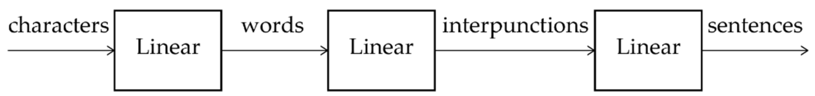
Figure 2.
Flow chart in linear systems. Upper panel: deterministic channel with multiplicative bias , Eq. (1). Lower panel: noisy deterministic channel with multiplicative bias and Gaussian noise source, Eq. (3).
Figure 2.
Flow chart in linear systems. Upper panel: deterministic channel with multiplicative bias , Eq. (1). Lower panel: noisy deterministic channel with multiplicative bias and Gaussian noise source, Eq. (3).
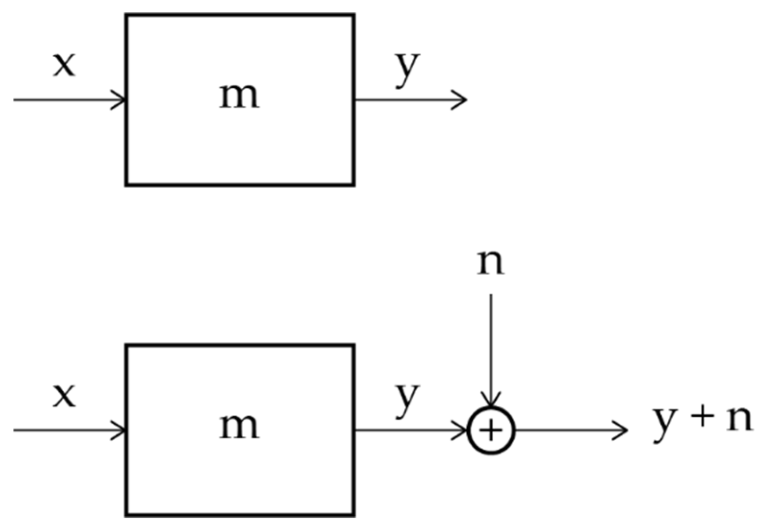
Figure 3.
Flow chart of variances: is the output variance of the values lying on the regression line, Eq. (7); is the output variance due to the values of not lying on the regression line, Eq. (6).
Figure 3.
Flow chart of variances: is the output variance of the values lying on the regression line, Eq. (7); is the output variance due to the values of not lying on the regression line, Eq. (6).
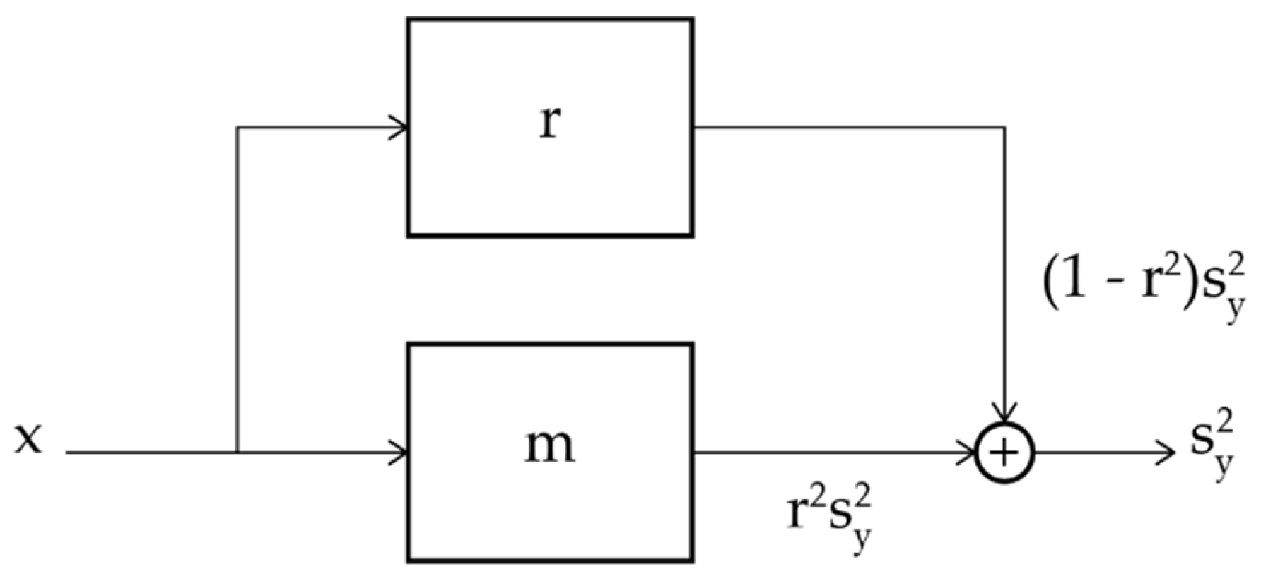
Figure 4.
Flow chart describing the cross channel.
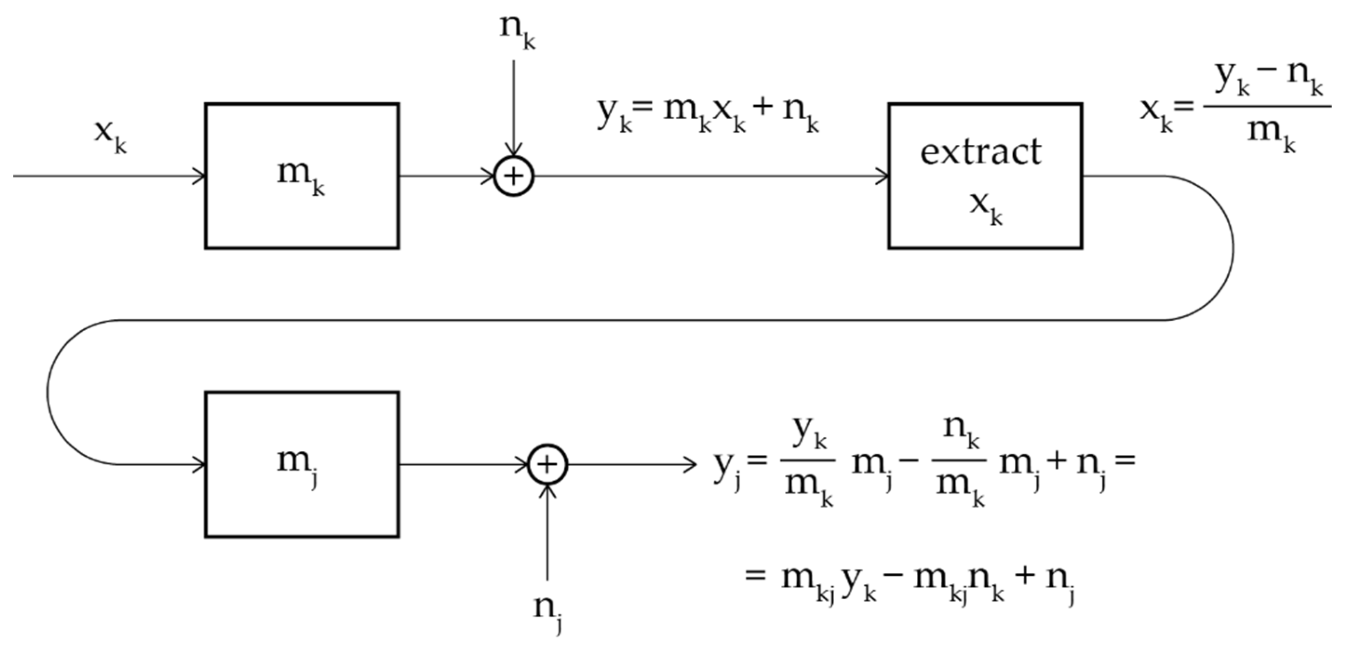
Figure 5.
Flow chart of noisy single channels connected in series.
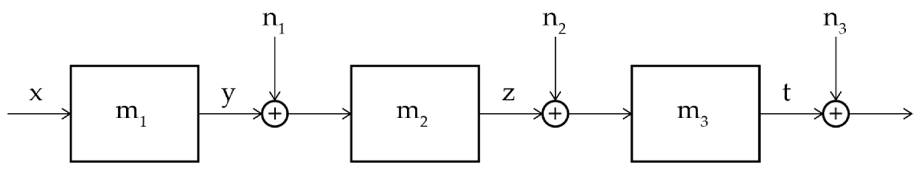
Figure 6.
Scatterplots in the original Greek texts between: (a) characters and words; (b) words and interpunctions; (c) interpunctions and sentences; (d) between characters and sentences.
Figure 6.
Scatterplots in the original Greek texts between: (a) characters and words; (b) words and interpunctions; (c) interpunctions and sentences; (d) between characters and sentences.
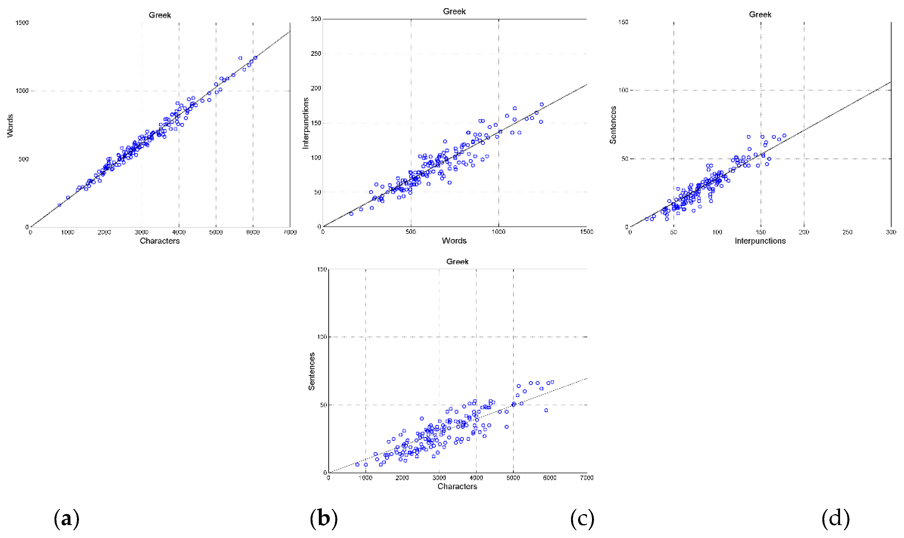
Figure 7.
Scatterplots in the English texts between: (a) characters and words; (b) words and interpunctions; (c) interpunctions and sentences; (d) between characters and sentences. In this case, English is the language to be translated.
Figure 7.
Scatterplots in the English texts between: (a) characters and words; (b) words and interpunctions; (c) interpunctions and sentences; (d) between characters and sentences. In this case, English is the language to be translated.
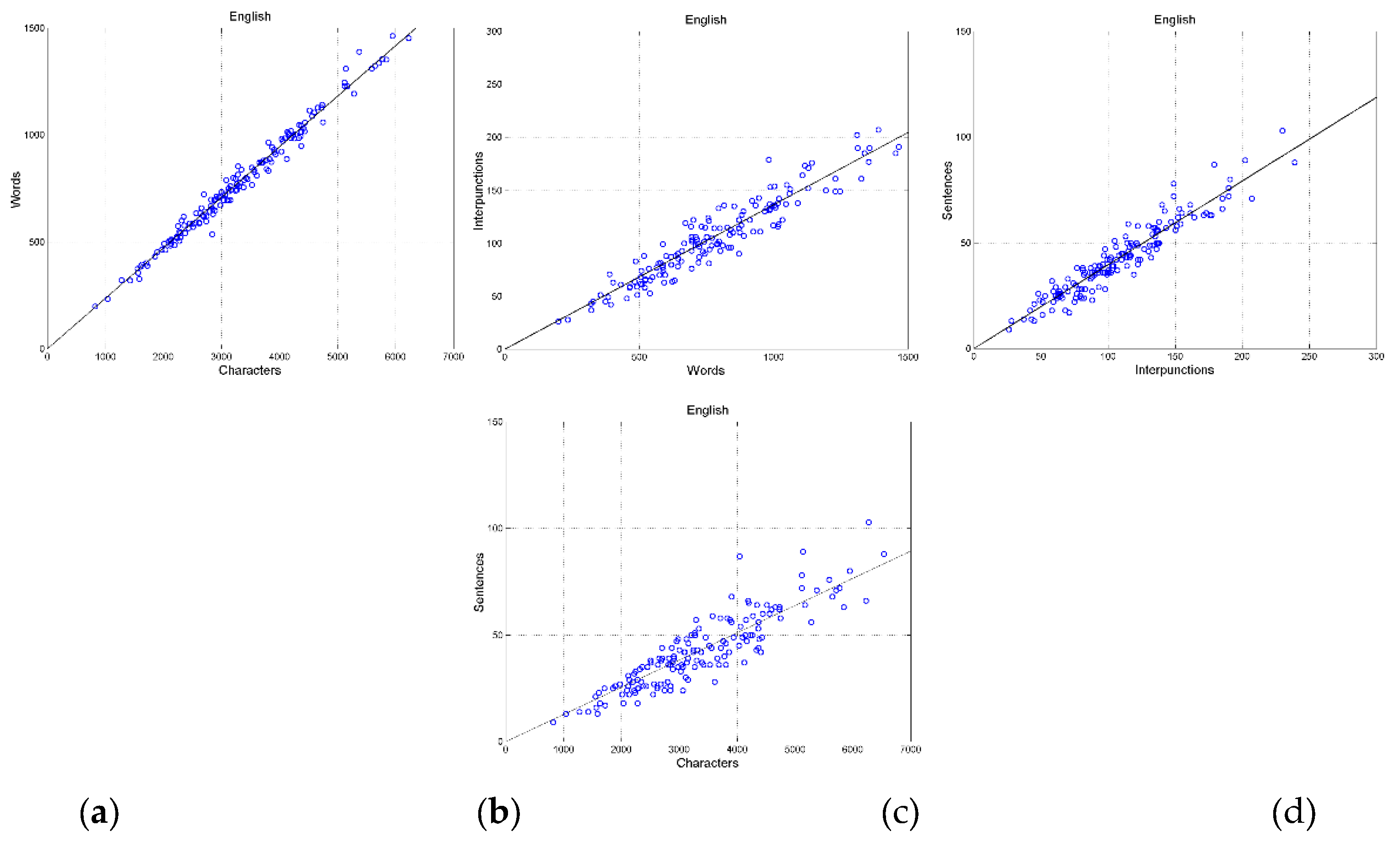
Figure 8.
(a) Probability distribution of the correlation coefficient ; (b) probability distribution of the coefficient of determination . Both refer to the following scatterplots: words versus characters, green; interpunctions versus words: cyan; sentences versus interpunctions, magenta. The black line refers to the scatterplot sentences versus characters; the red line refers to the series channel considered in Section 7.
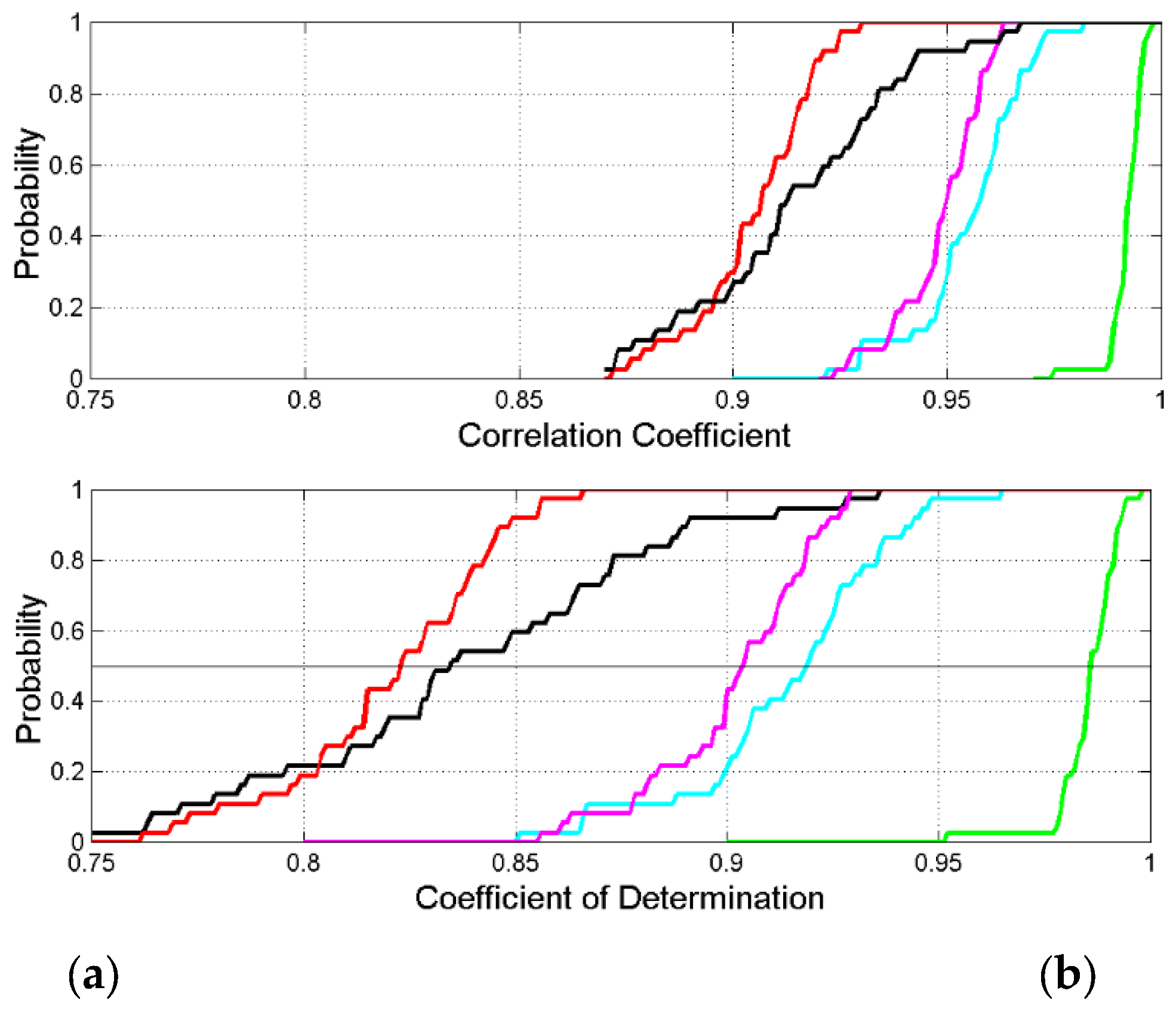
Figure 9.
Probability distribution of the regression line slope in the following scatterplots: words versus characters, green; interpunctions versus words: cyan; sentences versus interpunctions, magenta. The black line (not visible because superposed by the red cline) refers to the scatterplot sentences versus characters; the red line refers to the series channel considered in Section 7.
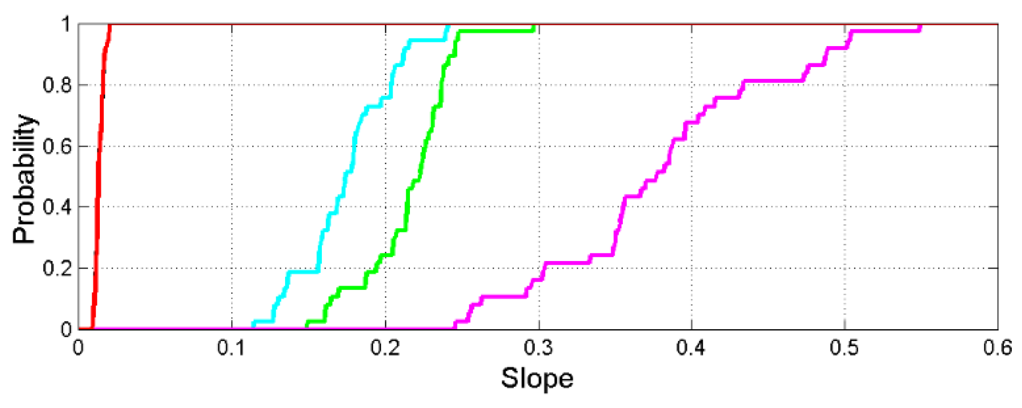
Figure 10.
(a) Signal–to–noise ratio SNR (dB) versus language (see order number in Table 1); (b) theoretical relationship between and the coefficient of determination. Characters–to–words, green; words–to–interpunctions, cyan; interpunctions–to–sentences, magenta. The horizontal lines in (a) draw mean values.
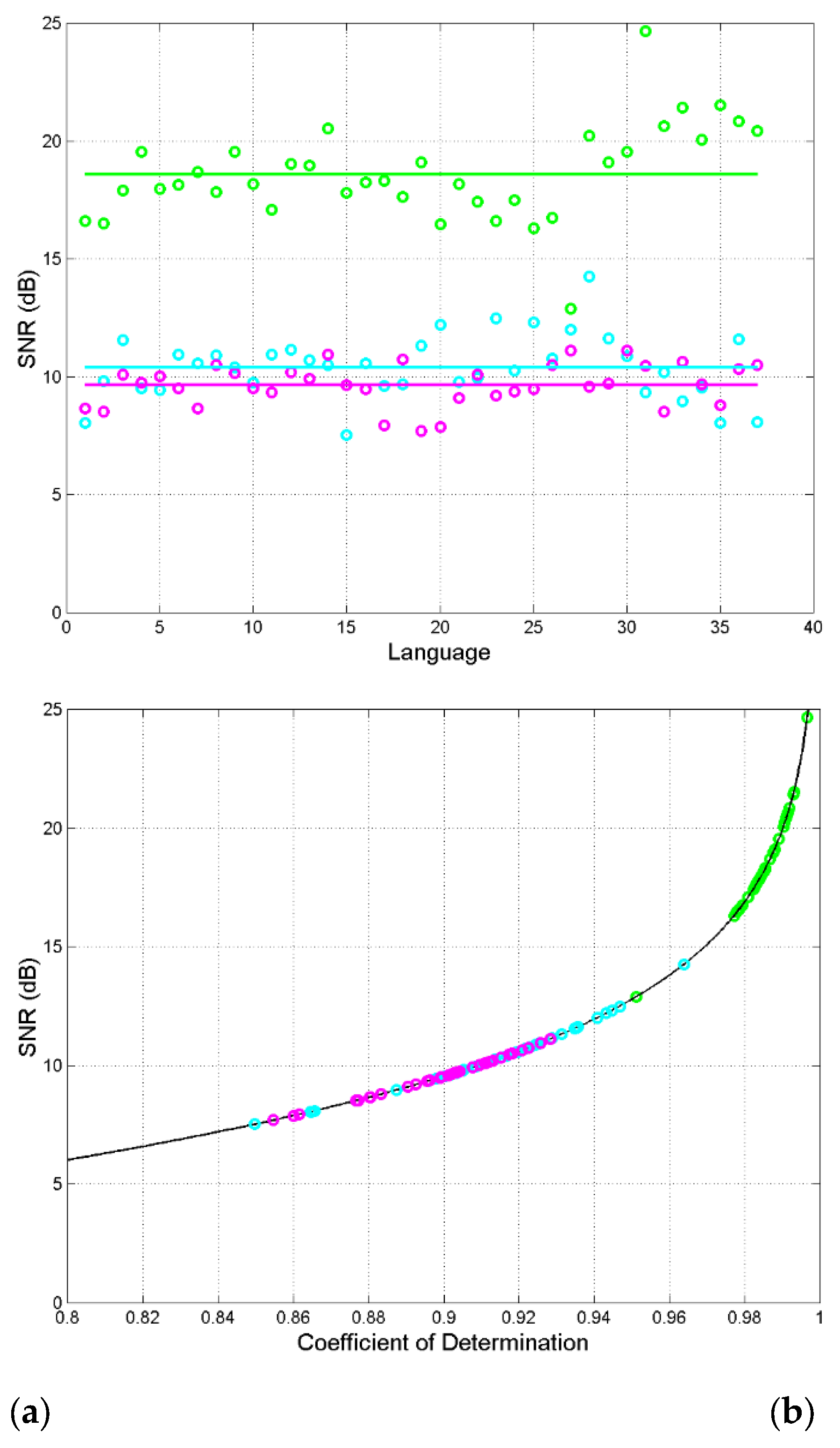
Figure 11.
Histograms (37 samples) of the signal–to–noise ratio SNR for each channel: (a) characters–to–interpunction; (b) words–to–interpunctions; (c) interpunctions–to–sentences.
Figure 11.
Histograms (37 samples) of the signal–to–noise ratio SNR for each channel: (a) characters–to–interpunction; (b) words–to–interpunctions; (c) interpunctions–to–sentences.
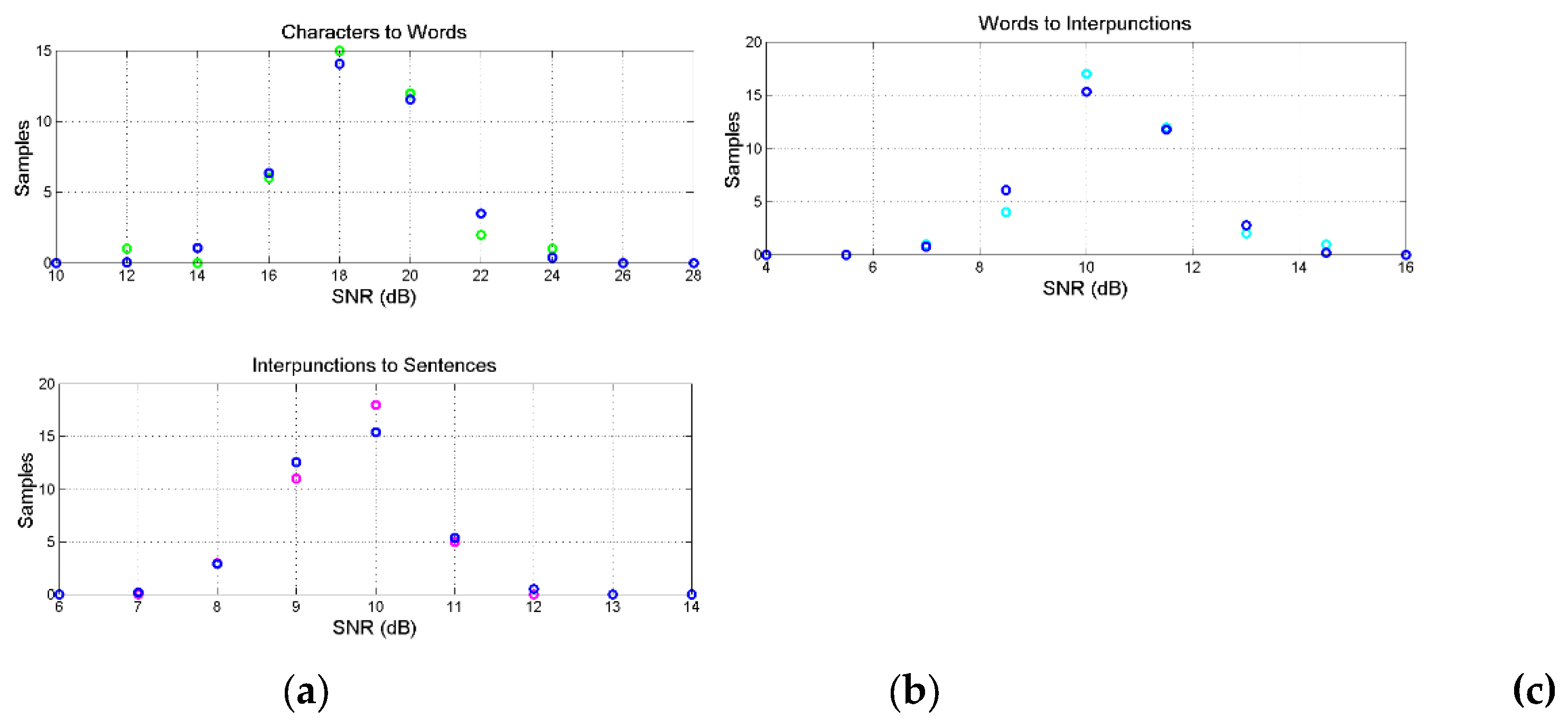
Figure 12.
Probability distribution of the the signal–to–noise ratio SNR in the following channels: characters–to–words, green; words–to–interpunctions, cyan; interpunctions–to–sentences, magenta. The black line refers to the channel characters–to–sentences estimated form the scatterplot of Figure 6(d); the red line refers to the series channel considered in Section 7.
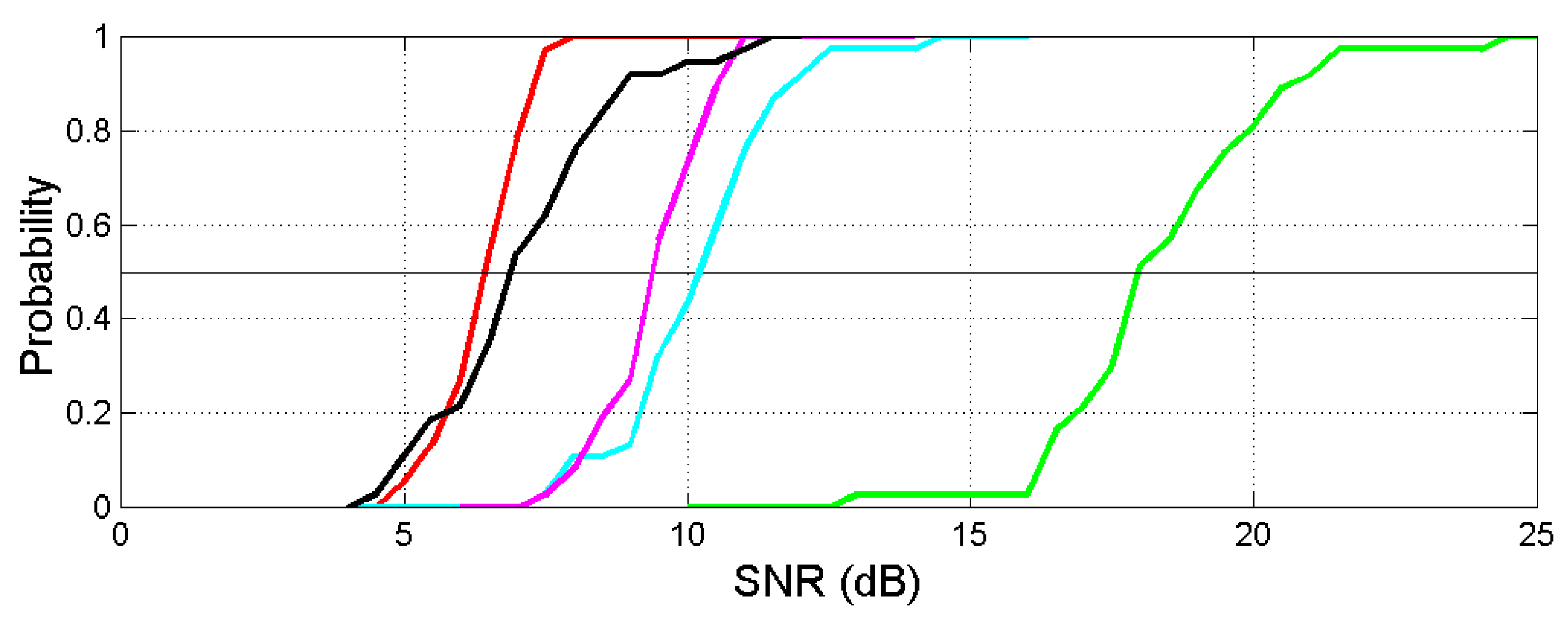
Figure 13.
(a) Single channel NSR and series channel NSR in linear units; (b) signal–to–noise ratio SNR (dB). The horizontal lines draw mean values. Channels: characters–to–words, green; words–to–interpunctions, cyan; interpunctions–to–sentences, magenta; series channel, red.
Figure 13.
(a) Single channel NSR and series channel NSR in linear units; (b) signal–to–noise ratio SNR (dB). The horizontal lines draw mean values. Channels: characters–to–words, green; words–to–interpunctions, cyan; interpunctions–to–sentences, magenta; series channel, red.
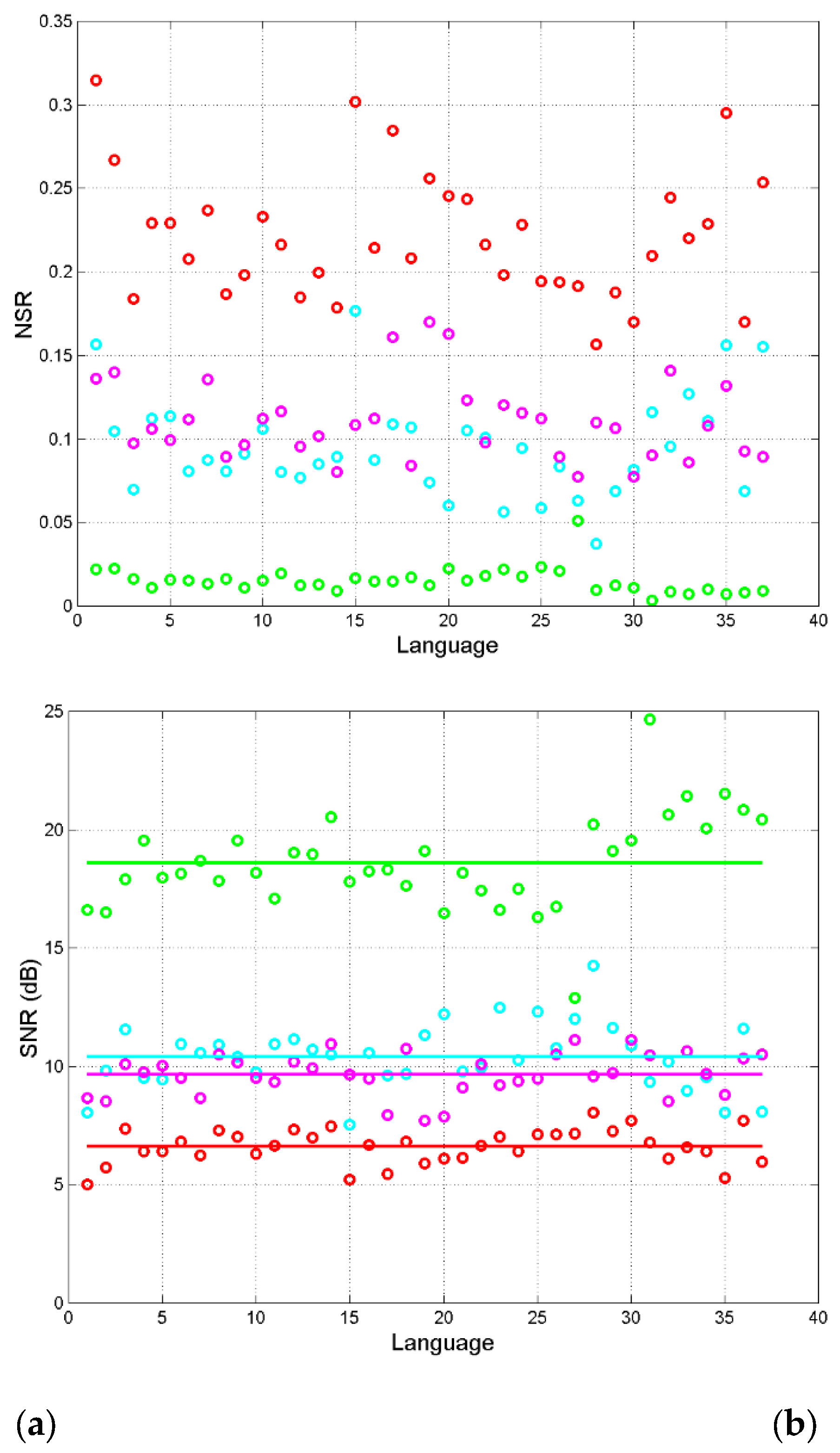
Figure 14.
(a) Scatterplot between the slope calculated from the scatterplot between characters and sentences (Table xx) and the slope given by Eq. (30); (b) Scatterplot between the correlation coefficient calculated from the scatterplot between characters and sentences (Table 2) and that calculated by solving Eq. (29) for the
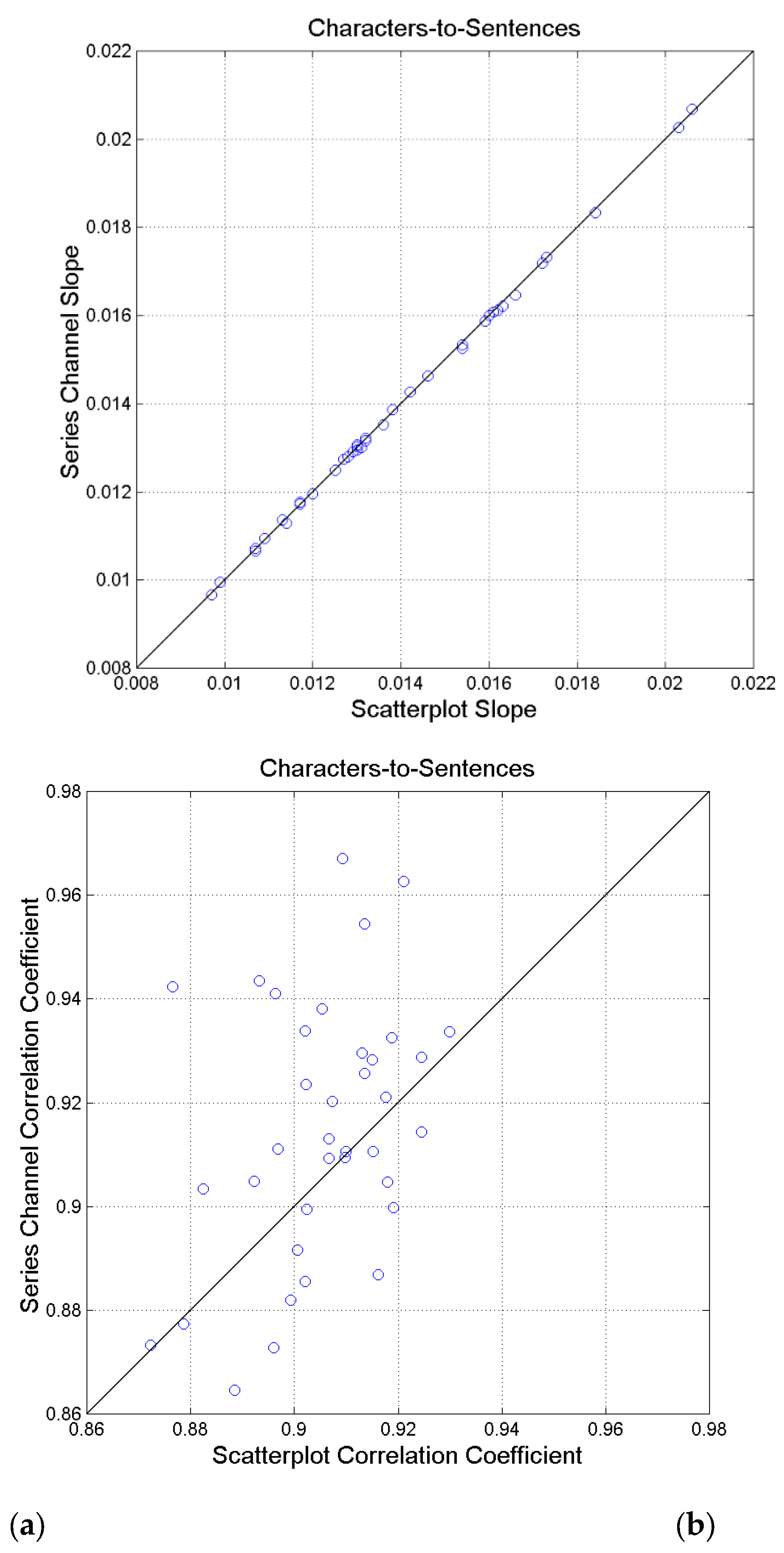
Figure 15.
Mean value (upper panel) and correlation coefficient (lower panel) in the indicated languages, assuming Greek as reference language (to be translated) in the channels: (a) words–to–words; (b) interpunctions–to–interpunctions; (c) sentences–to–sentences.
Figure 15.
Mean value (upper panel) and correlation coefficient (lower panel) in the indicated languages, assuming Greek as reference language (to be translated) in the channels: (a) words–to–words; (b) interpunctions–to–interpunctions; (c) sentences–to–sentences.
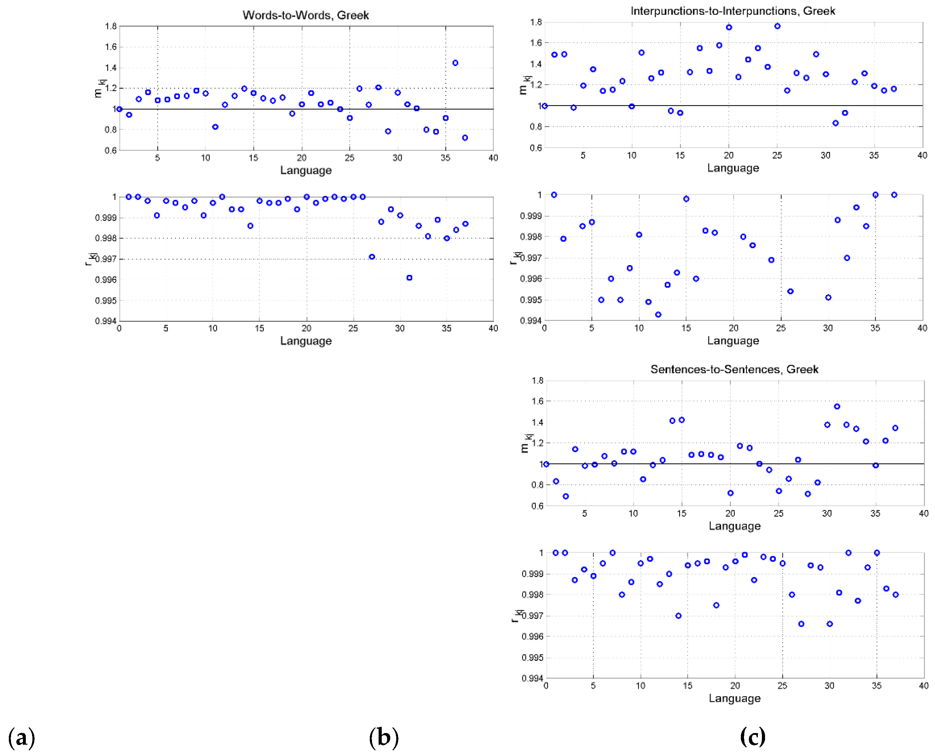
Figure 16.
Mean value (upper panel) and correlation coefficient (lower panel) in the indicated languages, assuming English as reference language (to be translated) in the channels: (a) words–to–words; (b) interpunctions–to–interpunctions; (c) sentences–to–sentences.
Figure 16.
Mean value (upper panel) and correlation coefficient (lower panel) in the indicated languages, assuming English as reference language (to be translated) in the channels: (a) words–to–words; (b) interpunctions–to–interpunctions; (c) sentences–to–sentences.
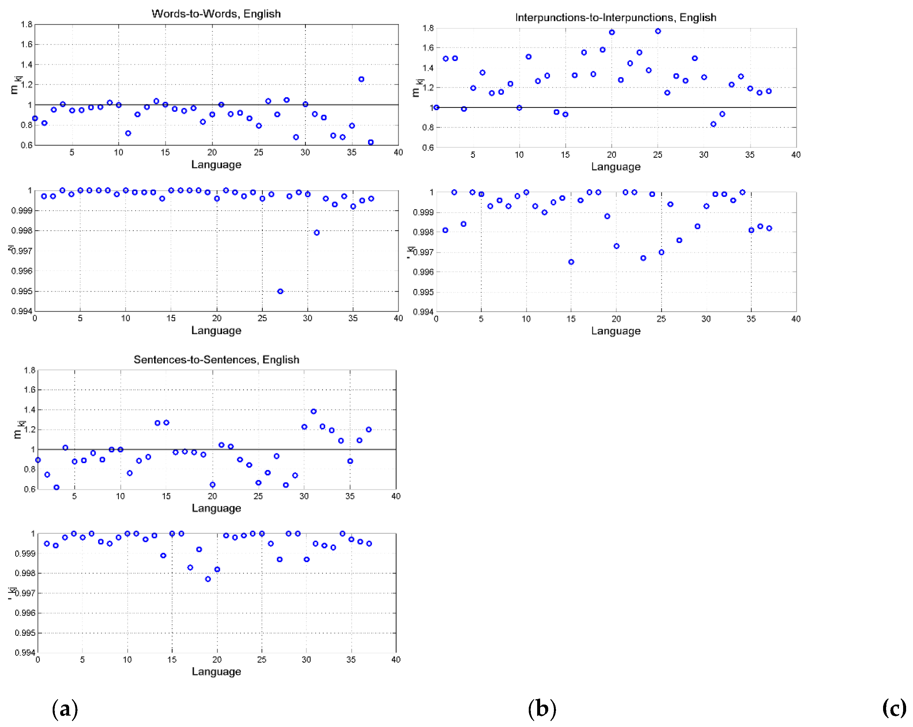
Figure 17.
Scatterplot between and in the indicated channels: (a) words–to–words; (b) interpunctions–to–interpunctions; (c) sentences–to–sentences. Red circles indicate the coordinates , of the barycenter.
Figure 17.
Scatterplot between and in the indicated channels: (a) words–to–words; (b) interpunctions–to–interpunctions; (c) sentences–to–sentences. Red circles indicate the coordinates , of the barycenter.
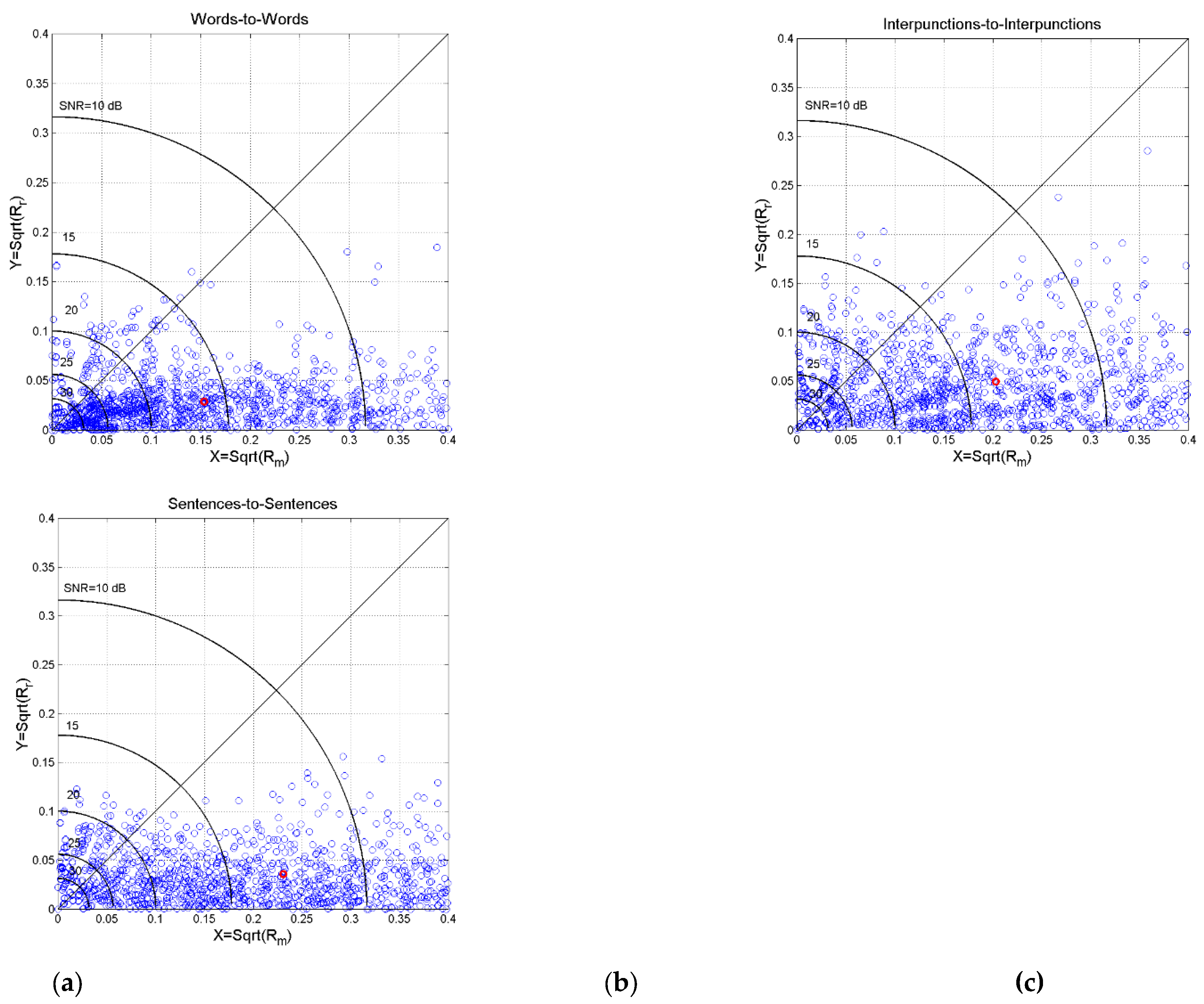
Figure 18.
Mean value (upper panel) and standard deviation lower of SNR (dB), in the indicated language (see Table 1), in the indicated channels: (a) words–to–words; (b) interpunctions–to–interpunctions; (c) sentences–to–sentences. Black lines indicate overall means. The mean of standard deviations is calculated from the mean of variances.
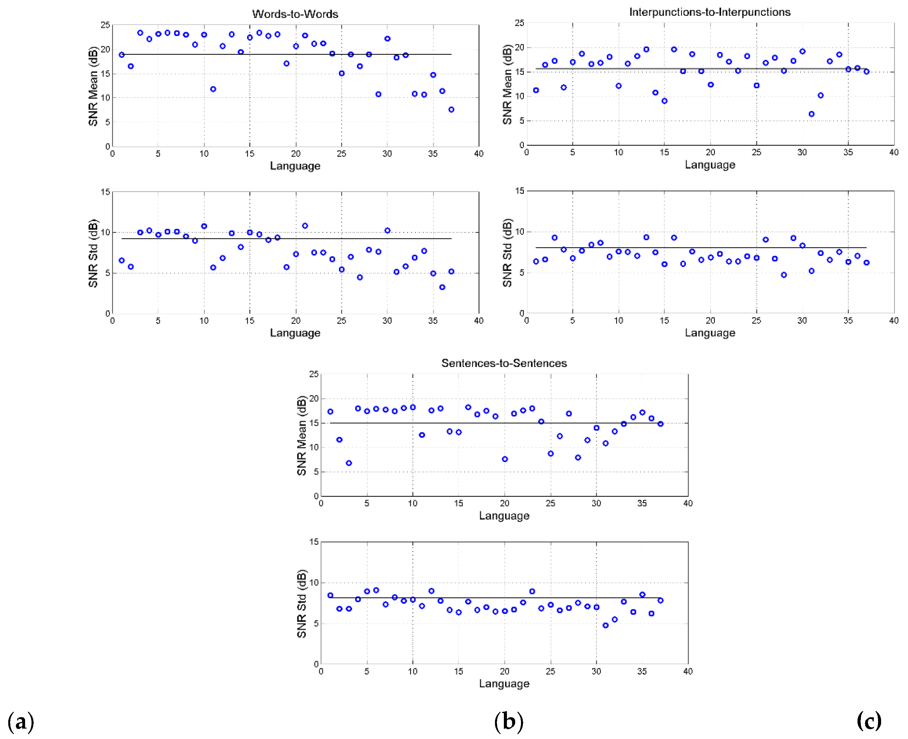
Figure 19.
Histogram of the signal–to–noise ratio SNR (dB) in the words–to–words channel ( samples), blue circles. The continuous black line models the histogram with a Gaussian density function.
Figure 19.
Histogram of the signal–to–noise ratio SNR (dB) in the words–to–words channel ( samples), blue circles. The continuous black line models the histogram with a Gaussian density function.
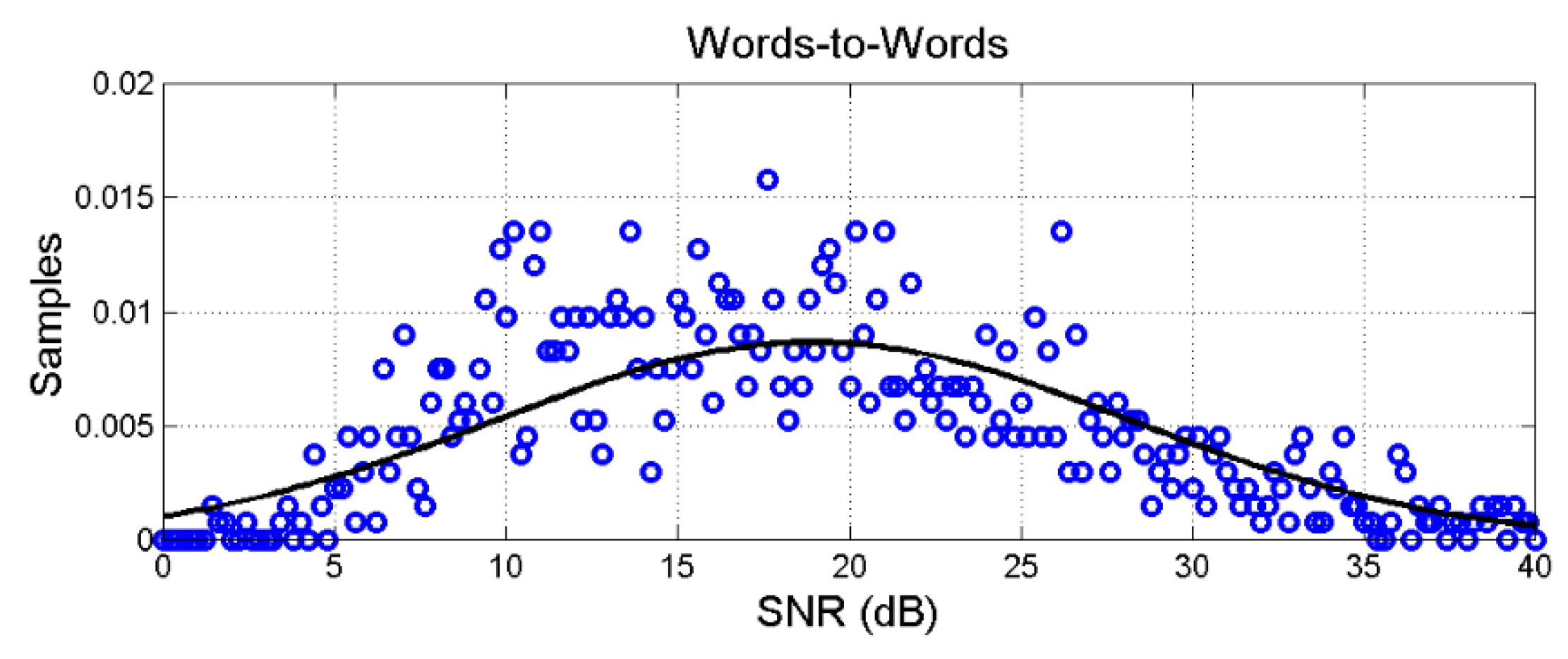
Figure 20.
“Universal” Gaussian probability density function (upper panel) and probability distribution function (that the abscissa is not exceeded) of (dB ) in the following channels: words–to–words, black; interpunctions–to–interpunctions, blue; sentences–to–sentences, red. The horizontal black line indicates the mean value.
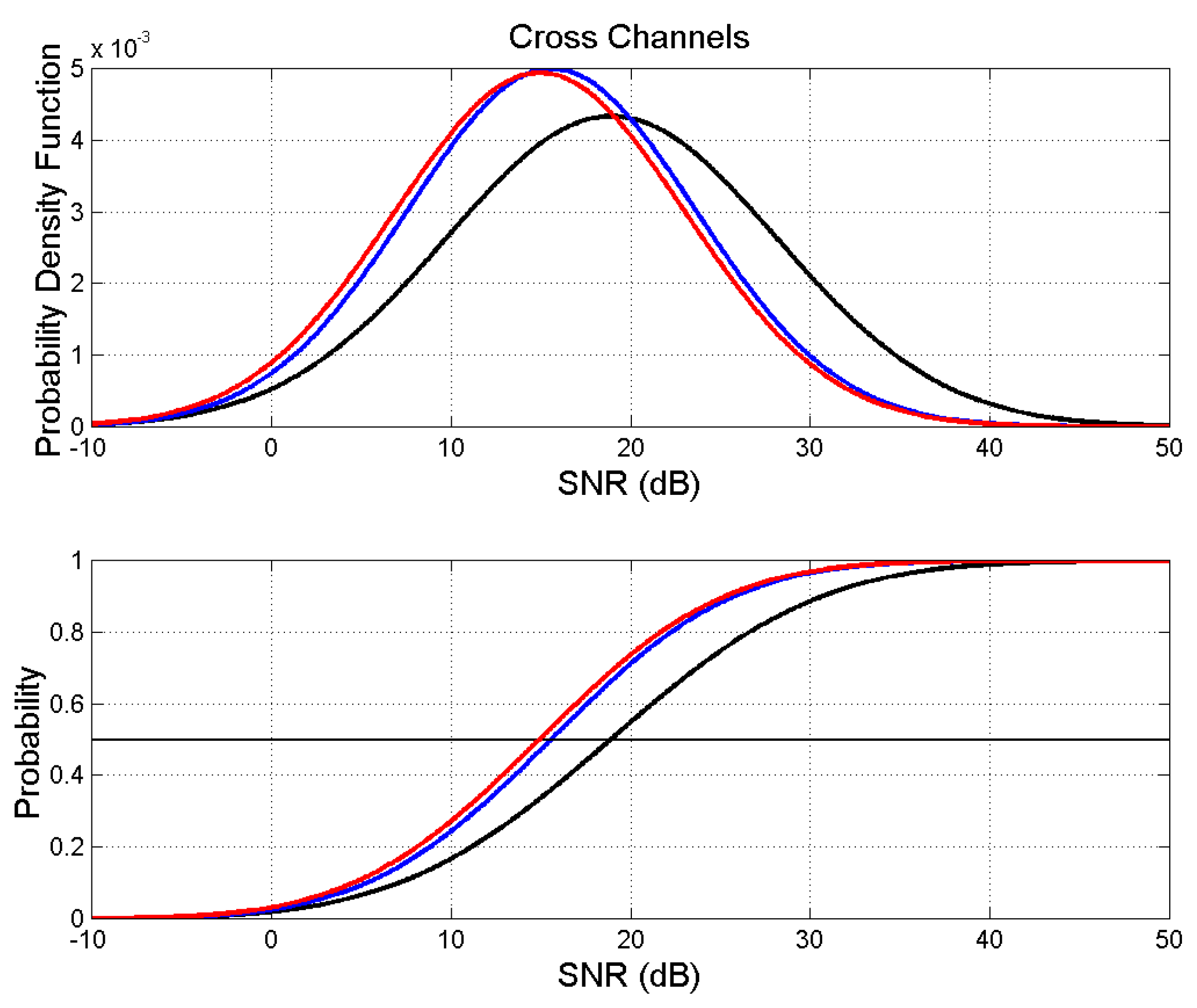

Table 1.
Language of translation and language family of the New Testament books (Matthew, Mark, Luke, John, Acts, Epistle to the Romans, Apocalypse), with total number of characters ( , words (, sentences () and interpunctions (). The list concerning the genealogy of Jesus of Nazareth reported in Matthew 1.1−1.17 17 and in Luke 3.23−3.38 was deleted for not biasing the statistics of linguistic variables [35]. The source of the texts considered is reported in Reference [35].
| Language | Order | Abbreviation | Language Family | |||||
|---|---|---|---|---|---|---|---|---|
| Greek | 1 | Gr | Hellenic | 486520 | 100145 | 4759 | 13698 | |
| Latin | 2 | Lt | Italic | 467025 | 90799 | 5370 | 18380 | |
| Esperanto | 3 | Es | Constructed | 492603 | 111259 | 5483 | 22552 | |
| French | 4 | Fr | Romance | 557764 | 133050 | 7258 | 17904 | |
| Italian | 5 | It | Romance | 505535 | 112943 | 6396 | 18284 | |
| Portuguese | 6 | Pt | Romance | 486005 | 109468 | 7080 | 20105 | |
| Romanian | 7 | Rm | Romance | 513876 | 118744 | 7021 | 18587 | |
| Spanish | 8 | Sp | Romance | 505610 | 117537 | 6518 | 18410 | |
| Danish | 9 | Dn | Germanic | 541675 | 131021 | 8762 | 22196 | |
| English | 10 | En | Germanic | 519043 | 122641 | 6590 | 16666 | |
| Finnish | 11 | Fn | Germanic | 563650 | 95879 | 5893 | 19725 | |
| German | 12 | Ge | Germanic | 547982 | 117269 | 7069 | 20233 | |
| Icelandic | 13 | Ic | Germanic | 472441 | 109170 | 7193 | 19577 | |
| Norwegian | 14 | Nr | Germanic | 572863 | 140844 | 9302 | 18370 | |
| Swedish | 15 | Sw | Germanic | 501352 | 118833 | 7668 | 15139 | |
| Bulgarian | 16 | Bg | Balto−Slavic | 490381 | 111444 | 7727 | 20093 | |
| Czech | 17 | Cz | Balto−Slavic | 416447 | 92533 | 7514 | 19465 | |
| Croatian | 18 | Cr | Balto−Slavic | 425905 | 97336 | 6750 | 17698 | |
| Polish | 19 | Pl | Balto−Slavic | 506663 | 99592 | 8181 | 21560 | |
| Russian | 20 | Rs | Balto−Slavic | 431913 | 92736 | 5594 | 22083 | |
| Serbian | 21 | Sr | Balto−Slavic | 441998 | 104585 | 7532 | 18251 | |
| Slovak | 22 | Sl | Balto−Slavic | 465280 | 100151 | 8023 | 19690 | |
| Ukrainian | 23 | Uk | Balto−Slavic | 488845 | 107047 | 8043 | 22761 | |
| Estonian | 24 | Et | Uralic | 495382 | 101657 | 6310 | 19029 | |
| Hungarian | 25 | Hn | Uralic | 508776 | 95837 | 5971 | 22970 | |
| Albanian | 26 | Al | Albanian | 502514 | 123625 | 5807 | 19352 | |
| Armenian | 27 | Ar | Armenian | 472196 | 100604 | 6595 | 18086 | |
| Welsh | 28 | Wl | Celtic | 527008 | 130698 | 5676 | 22585 | |
| Basque | 29 | Bs | Isolate | 588762 | 94898 | 5591 | 19312 | |
| Hebrew | 30 | Hb | Semitic | 372031 | 88478 | 7597 | 15806 | |
| Cebuano | 31 | Cb | Austronesian | 681407 | 146481 | 9221 | 16788 | |
| Tagalog | 32 | Tg | Austronesian | 618714 | 128209 | 7944 | 16405 | |
| Chichewa | 33 | Ch | Niger−Congo | 575454 | 94817 | 7560 | 15817 | |
| Luganda | 34 | Lg | Niger−Congo | 570738 | 91819 | 7073 | 16401 | |
| Somali | 35 | Sm | Afro−Asiatic | 584135 | 109686 | 6127 | 17765 | |
| Haitian | 36 | Ht | French Creole | 514579 | 152823 | 10429 | 23813 | |
| Nahuatl | 37 | Nh | Uto−Aztecan | 816108 | 121600 | 9263 | 19271 |
Table 2.
Slope and correlation coefficient , of the indicated regression lines in each language/translation.
Table 2.
Slope and correlation coefficient , of the indicated regression lines in each language/translation.
| Language | Words vs Characters | Interpunctions vs Words | Sentences vs Interpunctions | Sentences vs Characters. | ||||
| Greek | 0.2054 | 0.9893 | 0.1369 | 0.9298 | 0.3541 | 0.9382 | 0.0099 | 0.8733 |
| Latin | 0.1944 | 0.9890 | 0.2038 | 0.9515 | 0.2957 | 0.9366 | 0.0117 | 0.8646 |
| Esperanto | 0.2256 | 0.9920 | 0.2045 | 0.9668 | 0.2461 | 0.9545 | 0.0113 | 0.8998 |
| French | 0.2386 | 0.9945 | 0.1347 | 0.9483 | 0.4045 | 0.9509 | 0.0131 | 0.9339 |
| Italian | 0.2233 | 0.9921 | 0.1636 | 0.9476 | 0.3489 | 0.9537 | 0.0127 | 0.8856 |
| Portuguese | 0.2246 | 0.9924 | 0.1845 | 0.9620 | 0.3532 | 0.9484 | 0.0146 | 0.9106 |
| Romanian | 0.2312 | 0.9933 | 0.1568 | 0.9589 | 0.3823 | 0.9384 | 0.0138 | 0.8820 |
| Spanish | 0.2320 | 0.9919 | 0.1580 | 0.9619 | 0.3565 | 0.9581 | 0.0130 | 0.9047 |
| Danish | 0.2417 | 0.9945 | 0.1694 | 0.9574 | 0.3961 | 0.9551 | 0.0163 | 0.9257 |
| English | 0.2364 | 0.9925 | 0.1365 | 0.9509 | 0.3962 | 0.9483 | 0.0128 | 0.8916 |
| Finnish | 0.1702 | 0.9904 | 0.2067 | 0.9621 | 0.3029 | 0.9464 | 0.0107 | 0.9131 |
| German | 0.2142 | 0.9938 | 0.1731 | 0.9637 | 0.3511 | 0.9555 | 0.0130 | 0.9325 |
| Icelandic | 0.2315 | 0.9937 | 0.1805 | 0.9600 | 0.3672 | 0.9527 | 0.0154 | 0.9296 |
| Norwegian | 0.2460 | 0.9956 | 0.1305 | 0.9581 | 0.5018 | 0.9621 | 0.0162 | 0.9626 |
| Swedish | 0.2371 | 0.9918 | 0.1277 | 0.9218 | 0.5041 | 0.9499 | 0.0154 | 0.9423 |
| Bulgarian | 0.2271 | 0.9926 | 0.1809 | 0.9590 | 0.3861 | 0.9482 | 0.0159 | 0.9203 |
| Czech | 0.2223 | 0.9927 | 0.2125 | 0.9496 | 0.3879 | 0.9282 | 0.0184 | 0.9034 |
| Croatian | 0.2287 | 0.9915 | 0.1825 | 0.9504 | 0.3853 | 0.9605 | 0.0161 | 0.9095 |
| Polish | 0.1968 | 0.9939 | 0.2159 | 0.9650 | 0.3768 | 0.9245 | 0.0160 | 0.9049 |
| Russian | 0.2148 | 0.9889 | 0.2397 | 0.9712 | 0.2566 | 0.9274 | 0.0132 | 0.8728 |
| Serbian | 0.2370 | 0.9925 | 0.1745 | 0.9513 | 0.4154 | 0.9436 | 0.0172 | 0.9111 |
| Slovak | 0.2149 | 0.9911 | 0.1973 | 0.9532 | 0.4085 | 0.9544 | 0.0173 | 0.9092 |
| Ukrainian | 0.2181 | 0.9893 | 0.2122 | 0.9730 | 0.3556 | 0.9448 | 0.0166 | 0.9545 |
| Estonian | 0.2054 | 0.9912 | 0.1881 | 0.9559 | 0.3342 | 0.9467 | 0.0129 | 0.8995 |
| Hungarian | 0.1882 | 0.9885 | 0.2412 | 0.9719 | 0.2632 | 0.9482 | 0.0120 | 0.9282 |
| Albanian | 0.2458 | 0.9896 | 0.1573 | 0.9607 | 0.3040 | 0.9582 | 0.0117 | 0.9106 |
| Armenian | 0.2140 | 0.9753 | 0.1802 | 0.9699 | 0.3698 | 0.9635 | 0.0142 | 0.8868 |
| Welsh | 0.2482 | 0.9953 | 0.1734 | 0.9818 | 0.2543 | 0.9493 | 0.0109 | 0.9336 |
| Basque | 0.1614 | 0.9939 | 0.2045 | 0.9673 | 0.2925 | 0.9506 | 0.0097 | 0.9210 |
| Hebrew | 0.2380 | 0.9945 | 0.1784 | 0.9615 | 0.4869 | 0.9635 | 0.0206 | 0.9144 |
| Cebuano | 0.2149 | 0.9983 | 0.1145 | 0.9465 | 0.5491 | 0.9578 | 0.0136 | 0.9670 |
| Tagalog | 0.2072 | 0.9957 | 0.1281 | 0.9555 | 0.4879 | 0.9363 | 0.0130 | 0.9411 |
| Chichewa | 0.1649 | 0.9964 | 0.1685 | 0.9420 | 0.4733 | 0.9596 | 0.0132 | 0.9381 |
| Luganda | 0.1610 | 0.9951 | 0.1797 | 0.9488 | 0.4314 | 0.9501 | 0.0125 | 0.9235 |
| Somali | 0.1876 | 0.9965 | 0.1628 | 0.9300 | 0.3505 | 0.9399 | 0.0107 | 0.8773 |
| Haitian | 0.2972 | 0.9959 | 0.1571 | 0.9672 | 0.4338 | 0.9567 | 0.0203 | 0.9288 |
| Nahuatl | 0.1489 | 0.9955 | 0.1593 | 0.9304 | 0.4759 | 0.9582 | 0.0114 | 0.9435 |
| Overall | 0.0038 | 0.0252 | ||||||
Table 3.
Mean and standard deviation of the signal–to–noise ratio (dB) in the indicated channel. The probability density function of each channel is modelled as Gaussian.
Table 3.
Mean and standard deviation of the signal–to–noise ratio (dB) in the indicated channel. The probability density function of each channel is modelled as Gaussian.
| Channel | Mean Standard deviation of (dB) |
| Characters–to–Words | |
| Words–to–Interpunctions | |
| Interpunctions–to–Sentences |
Table 4.
Mean and standard deviation of the signal–to–noise ratio (dB) in the indicated cross channels. The probability density function of each channel is modelled as Gaussian.
Table 4.
Mean and standard deviation of the signal–to–noise ratio (dB) in the indicated cross channels. The probability density function of each channel is modelled as Gaussian.
| Channel | Mean (dB) | Standard Deviation (dB) |
| Words–to–Words | 18.93 | 9.21 |
| Interpunctions–to–Interpunctions | 15.60 | 7.99 |
| Sentences–to–Sentences | 14.94 | 8.08 |
Disclaimer/Publisher’s Note: The statements, opinions and data contained in all publications are solely those of the individual author(s) and contributor(s) and not of MDPI and/or the editor(s). MDPI and/or the editor(s) disclaim responsibility for any injury to people or property resulting from any ideas, methods, instructions or products referred to in the content. |
© 2025 by the authors. Licensee MDPI, Basel, Switzerland. This article is an open access article distributed under the terms and conditions of the Creative Commons Attribution (CC BY) license (http://creativecommons.org/licenses/by/4.0/).
Copyright: This open access article is published under a Creative Commons CC BY 4.0 license, which permit the free download, distribution, and reuse, provided that the author and preprint are cited in any reuse.


