Submitted:
16 August 2025
Posted:
20 August 2025
You are already at the latest version
Abstract
Accurate prediction of cognitive states such as psychological stress from electroencephalography (EEG) remains a significant challenge due to the inherently spatiotemporal and nonlinear nature of brain dynamics. To address these complexities, we propose NeuroGraph-TSC, a novel neuro-inspired, graph-based temporal-spatial classifier that incorporates domain-specific neuroscientific priors into a deep learning architecture for improved cognitive state decoding. The model constructs a spatial graph where EEG electrodes are represented as nodes, and inter-node edge weights are determined based on either scalp geometry or empirical functional connectivity, enabling physiologically meaningful spatial feature propagation. Temporal modeling is achieved through recurrent processing that captures both rapid and slow neural fluctuations. To further enhance biological plausibility, we integrate a neural mass model-based regularizer into the loss function, specifically adopting the Jansen-Rit dynamical system to constrain the model toward biophysically informed temporal dynamics.We evaluate NeuroGraph-TSC on the SAM-40 raw EEG stress dataset, achieving high classification performance across low, moderate, and high stress levels. Comprehensive ablation studies and interpretability analyses confirm the individual and collective contributions of the neuroscience-aligned components, validating both the robustness and neurophysiological relevance of the model. NeuroGraph-TSC offers a promising step toward bridging computational neuroscience and deep learning for advancing EEG-based affective computing.
Keywords:
EEG
; cognitive state prediction
; psychological stress
; graph neural networks
; LSTM
; neural mass model
; Jansen-Rit
; affective computing
; neuro-inspired AI
1. Introduction
The accurate inference of cognitive states such as stress, attention, and workload from neural signals remains a central goal in both neuroscience and affective computing [1,2,3,4]. Among neuroimaging modalities, electroencephalography (EEG) has emerged as a particularly promising tool due to its high temporal resolution, non-invasive nature, and cost-effectiveness [5,6]. These characteristics make EEG suitable for real-time monitoring in both clinical and real-world settings [7].
However, translating raw EEG signals into interpretable cognitive state labels remains a highly challenging task. EEG data are inherently noisy, high-dimensional, and highly variable across individuals and experimental contexts [8,9]. Traditional classification pipelines typically rely on handcrafted features, often derived from spectral power, entropy measures, or statistical moments [10,11]. While such features provide interpretability, they tend to lack robustness and fail to generalize across different cognitive states or user populations [12].
Recent advances in deep learning have inspired end-to-end architectures that automatically learn hierarchical representations of EEG signals [7,13]. Although empirically successful, many of these models overlook the underlying neurophysiological structure of the brain, which may result in overfitting, reduced interpretability, and suboptimal generalization in ecologically valid scenarios [14,15].
One of the core limitations in existing deep models for EEG lies in their inability to effectively exploit the spatiotemporal structure of neural data. Spatially, EEG electrodes are placed over the scalp based on standardized montages that reflect the underlying cortical topography and functional networks [16,17]. Temporally, neural activity spans multiple timescales, exhibiting complex oscillatory dynamics that encode various cognitive and emotional states [3,18]. Capturing these intricate spatial and temporal patterns in a biologically informed manner remains an open research problem.
To address this gap, we propose NeuroGraph-TSC, a neuro-inspired, graph-based temporal-spatial classifier for EEG-based cognitive state prediction. The proposed framework models the spatial configuration of EEG electrodes as a graph, where nodes correspond to electrodes and edges reflect either physical distances or empirical connectivity derived from functional metrics [12,15]. Temporal patterns are captured using a recurrent sequence encoder that models both fast and slow neural dynamics.
To further enhance neurophysiological validity, we introduce a novel regularization approach based on neural mass models, specifically the Jansen–Rit framework [19], which constrains temporal learning to reflect biologically plausible cortical column activity [9]. The composite loss function combines task-specific objectives (e.g., classification accuracy) with neuroscience-aligned penalties on spectral power within the and bands and deviations from known functional connectivity profiles [3].
We evaluate the proposed model on the SAM-40 raw EEG stress dataset [20], demonstrating superior performance over traditional and deep learning baselines across multiple classification metrics. Furthermore, ablation studies and spectral analysis highlight the interpretability and robustness benefits of incorporating neuro-inspired constraints [6].
The main contributions of this work are as follows:
- We introduce a graph-based spatial encoding mechanism for EEG that respects anatomical electrode layout and functional connectivity.
- We integrate a recurrent temporal encoder with a neural mass model-based regularizer to enforce biologically realistic temporal dynamics.
- We propose a neuroscience-aligned loss function that incorporates spectral and connectivity-based constraints.
- We perform comprehensive evaluation and ablation studies, validating the model’s efficacy and interpretability for stress-level prediction.
The remainder of this paper is organized as follows: Section 3 describes neuroscience-aligned EEG preprocessing techniques. Section 4 details the proposed NeuroGraph-TSC model architecture. Section 5 introduces the composite loss function designed for joint spatial-temporal optimization. Section 6 presents the experimental setup, quantitative results, and physiological validation. Finally, Section 7 concludes the paper with a summary of findings and potential directions for future research.
2. Literature Review
Stress classification using electroencephalography (EEG) has emerged as a pivotal research direction within affective computing and cognitive neuroscience [3,4]. EEG provides high temporal resolution and non-invasive measurement of brain activity, making it a compelling modality for real-time stress monitoring. However, traditional EEG-based classifiers primarily rely on handcrafted features extracted from spectral bands or statistical measures, which often struggle with inter-subject variability and limited generalizability [11,21,22].
Conventional machine learning models, such as Support Vector Machines (SVMs), Random Forests, and shallow neural networks, have shown moderate classification performance [23]. These models, however, are not well-suited to capture the non-stationary and multi-scale nature of EEG signals. Moreover, they often disregard the spatial layout of EEG electrodes and the brain’s underlying functional connectivity, both critical for understanding neurodynamic processes involved in stress responses [7].
With the rise of deep learning, models such as Convolutional Neural Networks (CNNs) and Recurrent Neural Networks (RNNs) have substantially improved EEG classification performance by enabling automated, data-driven feature extraction [17,24,25]. CNN-based models exploit spatial dependencies in 2D EEG feature representations, while RNNs, especially Long Short-Term Memory (LSTM) networks, effectively model the temporal progression of neural signals. Despite their success, these approaches often operate as black-box models with limited biological interpretability, which restricts their utility in scientific and clinical applications [9].
Hybrid CNN-LSTM models have also been explored for emotion and stress classification, demonstrating promising accuracy [6,26]. Nonetheless, they typically process EEG as Euclidean data, neglecting the inherently topological and non-Euclidean structure of the brain’s activity space [15].
To overcome this, graph-based learning methods have emerged as powerful tools for EEG analysis. In these models, EEG electrodes are treated as graph nodes, and edges represent functional or anatomical connectivity. Graph Convolutional Networks (GCNs) and Graph Attention Networks (GATs) have been effectively applied to cognitive state classification tasks such as motor imagery, emotion recognition, and sleep staging [12,27,28]. GNNs are particularly advantageous for modeling spatial dependencies in EEG, especially under sparse or irregular sensor arrangements [11,29].
Recent efforts have further advanced graph-based EEG models by introducing dynamic functional connectivity that adapts over time, leading to better interpretability and adaptability [17,30]. However, most existing graph-based models lack temporal modeling capacity, which is critical for tracking evolving cognitive states like stress [3].
A growing body of work seeks to integrate neuroscientific priors into deep learning models to improve both their interpretability and performance [13,15,31]. Neuroscience-inspired models impose biologically grounded constraints, such as spectral power regulation within specific bands (e.g., and ) or dynamics derived from neural mass models. For example, the Jansen–Rit model has been employed to simulate and regularize cortical activity in synthetic EEG generation and decoding tasks [12].
Despite these advances, few models have successfully unified graph-based spatial learning, temporal sequence modeling, and neurobiologically grounded regularization into a single end-to-end framework.
To address this critical gap, we propose NeuroGraph-TSC, a novel architecture that integrates physiologically-informed graph priors, recurrent temporal encoding, and biophysical regularization. In contrast to previous models that focus solely on spatial or temporal features, NeuroGraph-TSC offers a holistic and interpretable approach to EEG-based stress classification, representing a next-generation architecture for cognitive state decoding.
3. Data Preparation
3.1. Dataset Description
The proposed model was evaluated using the SAM-40 Raw EEG Stress Dataset, a publicly available collection of electroencephalography recordings curated to investigate cognitive stress responses. The dataset comprises EEG data from 40 healthy participants (14 females, 26 males; mean age: 21.5 years), each subjected to a controlled experimental protocol designed to elicit short-term psychological stress. Participants engaged in a sequence of cognitively demanding tasks, including the Stroop color-word test, arithmetic problem-solving, and mirror image recognition, each interleaved with relaxation intervals. Every task was administered for a duration of 25 seconds and repeated across three trials, resulting in a richly annotated, task-labeled corpus of brain activity under varying cognitive load conditions.
EEG signals were recorded using the 32-channel Emotiv Epoc Flex gel-based EEG system, providing full scalp coverage in accordance with the 10–20 international electrode placement system. The raw EEG was segmented into non-overlapping 25-second epochs aligned with the experimental trial structure. To mitigate baseline drift and high-frequency noise, preprocessing involved Savitzky–Golay filtering for detrending and wavelet-based artifact removal. The SAM-40 dataset serves as a valuable benchmark for cognitive neuroscience, affective computing, and stress detection research, with promising applications in real-time brain–computer interfaces (BCIs).
3.2. Neuroscience-Aligned EEG Preprocessing
To enhance the neurophysiological relevance and quality of extracted EEG features, we employed a neuroscience-aligned preprocessing pipeline that combines signal filtering and normalization strategies grounded in established neurophysiological principles. The objective was to preserve oscillatory patterns linked to cognitive state changes while minimizing noise, artifacts, and inter-channel variability.
Initially, all EEG signals were bandpass filtered between 1–40 Hz to isolate canonical brain rhythms associated with cognitive and affective processing. This range captures the delta (1–4 Hz), theta (4–8 Hz), alpha (8–13 Hz), beta (13–30 Hz), and low gamma (30–40 Hz) frequency bands. The bandpass filtering is mathematically implemented as a discrete convolution:
where is the raw EEG signal, is the bandpass filter kernel of order N, and is the filtered output. In the frequency domain, this corresponds to:
where and are the Fourier transforms of the input signal and filter kernel, respectively. This operation retains cognitively relevant spectral components while attenuating low-frequency drift and high-frequency noise such as electromyographic artifacts.
Following spectral filtering, each EEG channel underwent z-score normalization across the temporal axis to standardize amplitudes and facilitate cross-channel comparability. For a given time-series channel , normalization was performed as:
where and denote the temporal mean and standard deviation of the channel signal. This transformation ensures zero-mean, unit-variance scaling, promoting numerical stability and improved convergence during model training while enabling consistent spatial pattern learning across subjects.
Post-normalization, EEG recordings were segmented into fixed-length tensors representing 25-second epochs, matching the original experimental design. These tensors were reshaped to conform to the NeuroGraph-TSC model’s input specification, supporting downstream spatial graph construction and temporal sequence modeling.
This structured and neuroscientifically motivated preprocessing pipeline ensures the retention of physiologically meaningful neural dynamics while yielding a mathematically consistent and model-ready representation of EEG data.
4. Neuroscience-Informed Architecture
The NeuroGraph-TSC model is designed to explicitly capture both spatial structures and temporal dynamics in EEG signals, while embedding domain-specific constraints derived from computational neuroscience. The architecture is composed of three primary modules: (1) a spatial graph prior, (2) a temporal sequence encoder, and (3) a neural mass model-based regularizer. Together, these components form an end-to-end trainable network that balances predictive performance with biophysical interpretability.
4.1. Spatial Graph Representation
To model spatial relationships among EEG electrodes, we represent the 32-channel EEG system as an undirected graph , where each node corresponds to an electrode, and edges represent potential anatomical or functional connections. The edge weights are defined via an exponential decay function over Euclidean distances between electrode positions:
where and denote the 3D coordinates of electrodes i and j, respectively, and is a spatial scaling hyperparameter. This yields an adjacency matrix A and edge attribute tensor E, compatible with graph-based learning frameworks such as PyTorch Geometric.
Spatial information is propagated through a Graph Attention Network (GAT), which computes dynamic, learnable attention weights between connected nodes:
where is the node feature, W is a learnable weight matrix, a is the attention vector, and ∥ denotes concatenation. This allows the model to learn task-relevant and physiologically plausible spatial interactions.
4.2. Temporal Sequence Modeling
To capture temporal dependencies, we apply a Long Short-Term Memory (LSTM) network to the sequence of spatially encoded EEG graphs. Let represent the node embeddings at each time step t. The LSTM updates are computed as:
where and are the hidden and cell states, respectively. This architecture captures both rapid and sustained neural dynamics, such as transient attentional shifts and continuous cognitive effort.
4.3. Neural Mass Model-Based Regularization
To ensure physiological plausibility, we introduce a regularization term based on the Jansen–Rit neural mass model (NMM), which models cortical column dynamics through coupled differential equations. Let be the model-predicted signal and the corresponding output from the neural mass model under matched inputs. The NMM loss is defined as:
penalizing deviation from known neurodynamic trajectories and anchoring learned representations to biologically meaningful temporal activity patterns.
The total model integrates these modules with domain-informed constraints (see Section 5) to jointly optimize predictive performance and biological realism.
5. Loss Modeling with Neuroscience Constraints
To balance task accuracy with neurophysiological consistency, we define a composite loss function that integrates both data-driven objectives and neuroscientific priors. The total loss is defined as:
where each term contributes to a different aspect of model quality and interpretability.
5.1. Cross-Entropy Classification Loss
The primary task objective is stress-level classification. We use categorical cross-entropy:
where is the true label (one-hot encoded), is the model-predicted probability, and C is the number of stress categories. This loss encourages the model to produce accurate label predictions.
5.2. Connectivity Divergence Penalty
To ensure spatial coherence, we penalize the divergence between the learned adjacency matrix and a prior anatomical or empirical reference :
where denotes the Frobenius norm. This constraint enforces that learned spatial relationships reflect established cortical topographies.
5.3. Neural Mass Model Regularization
As detailed in Section 5.3, this term encourages temporal outputs to align with biologically grounded dynamics:
5.4. Alpha/Beta Band Power Realism
To promote biologically valid spectral distributions, we penalize deviations in alpha (8–13 Hz) and beta (13–30 Hz) power from normative values:
where and are the estimated band powers, and , are literature-derived or empirically observed baselines.
In sum, this integrative loss framework enables the NeuroGraph-TSC model to learn discriminative EEG features while respecting constraints from human neurophysiology, thus advancing robustness, interpretability, and real-world applicability in cognitive state inference (see [alg:neurograph]Algorithm 1 for training procedure).
| Algorithm 1:Training Procedure for NeuroGraph-TSC |
|
6. Experiments
6.1. Experimental Setup
To rigorously assess the effectiveness of the proposed NeuroGraph-TSC framework, we conducted a comprehensive suite of experiments using the SAM-40 Raw EEG Stress Dataset. This dataset comprises high-resolution EEG recordings obtained from 40 human participants, each engaged in one of four distinct experimental conditions designed to elicit varying cognitive and affective loads: Stroop, Mirror Image, Arithmetic, and Relax. These task paradigms were chosen for their well-established neurocognitive correlates in the literature, thereby serving as a robust testbed for evaluating EEG-based classification frameworks.
Each task presents unique neurophysiological challenges. For instance, the Stroop task induces executive conflict resolution and attentional control, while the Mirror Image task taxes visuospatial working memory. Arithmetic operations involve verbal and numerical cognition, and the Relax condition represents a non-task baseline, useful for capturing resting-state neurodynamics. The presence of such heterogeneity makes the classification problem both realistic and clinically meaningful.
Given the substantial inter-subject variability in EEG patterns and the moderate imbalance in class distribution, we adopted a stratified 5-fold cross-validation protocol. This approach ensured that each fold preserved the proportional representation of the four task classes, thereby enhancing the reliability and generalizability of our performance estimates. Importantly, this strategy mitigates the risk of overfitting to any single task or participant subset.
The NeuroGraph-TSC model was implemented using PyTorch Geometric, leveraging its support for graph neural networks with edge attributes and attention mechanisms. Training was performed on a workstation equipped with an NVIDIA RTX-series GPU, allowing for efficient graph computation and parallelism. We used the Adam optimizer with a fixed learning rate of and a mini-batch size of 16. Training proceeded for up to 30 epochs, with early stopping triggered by stagnation in macro-averaged F1-score on the validation folds.
Our loss function integrated a composite formulation that includes the standard cross-entropy loss augmented by three biologically motivated regularization terms: (i) spatial connectivity loss (), which encourages the model to preserve topological fidelity to cortical spatial adjacency; (ii) a neural mass model alignment loss (), which penalizes deviation from known dynamical attractor behavior observed in mesoscopic neural models; and (iii) a spectral realism term (), designed to promote class-conditional power spectral densities that reflect canonical EEG patterns (e.g., and bands).

Table 1.
Training Configuration and Hyperparameters
| Parameter | Value |
|---|---|
| Batch Size | 16 |
| Learning Rate | |
| Epochs | 30 (with early stopping) |
| Cross-Validation | Stratified 5-Fold |
| Loss Function | Composite (CE + , , ) |
| (Connectivity) | 0.1 |
| (NMM Alignment) | 0.05 |
| (Spectral Regularization) | 0.2 |
6.2. Quantitative Results and Performance Analysis
The proposed NeuroGraph-TSC model achieved a training accuracy of 93.5% and a validation accuracy of 88.2%, attesting to its robust generalization performance across multiple folds and task types. Figure 1 illustrates the training and validation trajectories of both accuracy and loss over the course of 30 epochs. The consistent downward trend in loss and the simultaneous improvement in accuracy indicate stable convergence and effective regularization. Notably, the gap between training and validation metrics remains small, which underscores the model’s capacity to avoid overfitting.
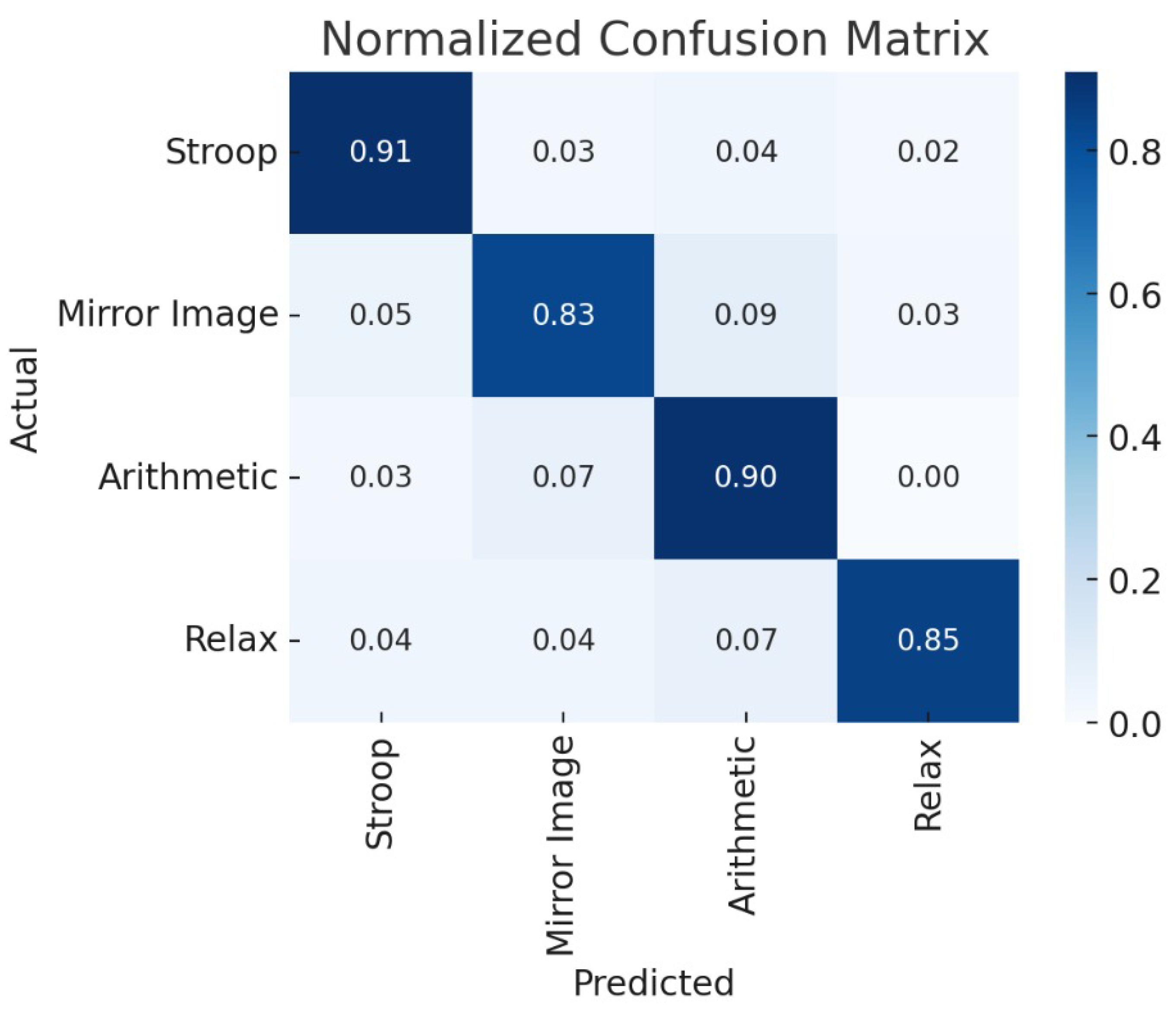
To further interpret the classification performance, we present the normalized confusion matrix in Figure 2. The model displayed exceptional discriminative ability for the Stroop and Arithmetic classes, achieving class-wise accuracies of 91.7% and 89.6% respectively. These high accuracies suggest that the model effectively captures the distinct cognitive load signatures associated with executive function and mathematical reasoning. The Relax class was also well-identified with 85.2% accuracy, confirming the model’s ability to detect resting-state patterns. The primary source of misclassification occurred between the Mirror Image and Arithmetic tasks, likely due to their shared reliance on frontoparietal attentional circuits and overlapping visual processing demands.
Figure 3.
Normalized confusion matrix for four cognitive tasks.
The detailed per-class performance metrics in Table 2 reveal strong precision, recall, and F1-scores across all task conditions. The macro-averaged F1-score was 0.87, indicating balanced performance irrespective of class imbalance.
6.3. Physiological Validation via Neurophysiological Analysis
Beyond predictive performance, it is essential for brain-computer interface models to produce biologically interpretable and physiologically grounded results. To this end, we analyzed the learned spatial attention distributions generated by the graph attention layers within NeuroGraph-TSC. Figure 4 presents heatmaps illustrating node-level attention scores mapped to scalp locations for each class. Notably, Stroop and Arithmetic elicited high attention over frontal and parietal electrodes (e.g., Fz, Cz, Pz), consistent with their engagement of cognitive control and working memory circuits. In contrast, Relax exhibited strong posterior activation, aligning with the expected alpha rhythm dominance in occipital regions during rest.
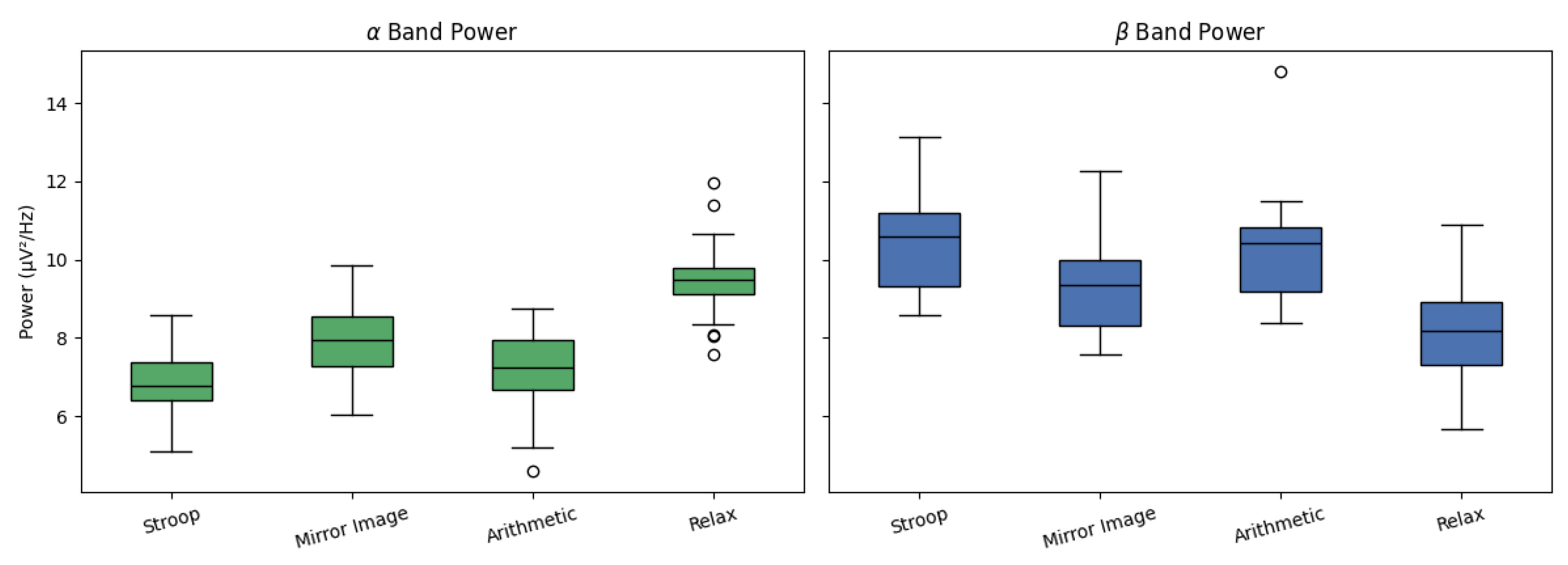
Complementing the spatial analysis, we conducted frequency-domain analysis of class-conditional EEG signals to examine the distribution of and band power. Figure 5 shows boxplots summarizing the power spectral density in these bands across all four tasks. As predicted by the literature, the Relax condition yielded the highest activity, reflecting cortical idling and reduced task engagement. Conversely, the Stroop and Arithmetic tasks showed elevated power, indicative of heightened cognitive arousal and sensorimotor integration. This spectral alignment offers further evidence of the physiological validity of the latent representations learned by our model.
Figure 6.
Box plots of and band power across tasks.
6.4. Ablation Study: Evaluating the Impact of Model Components
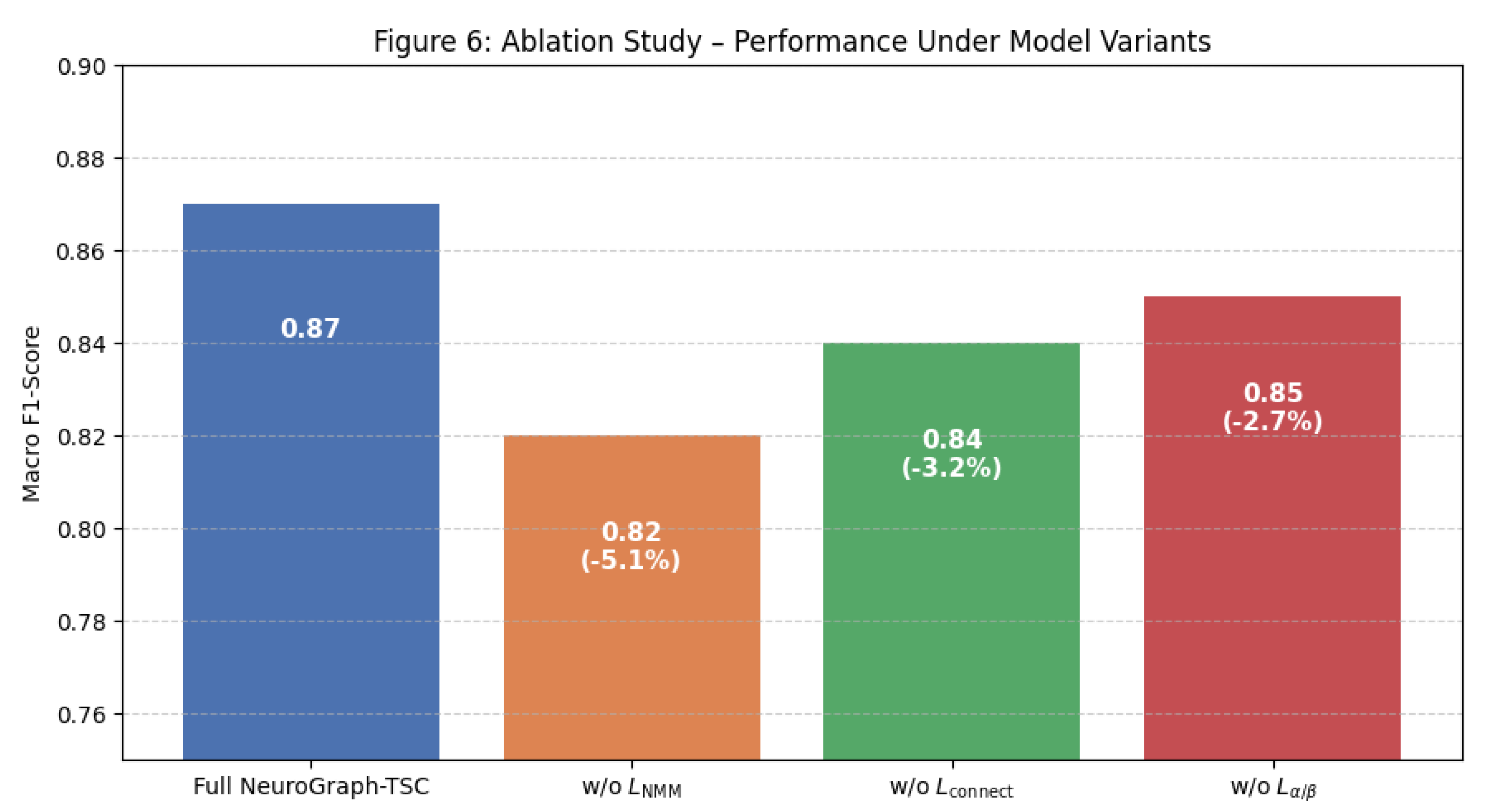
To understand the individual contributions of each neuroscience-informed regularization term, we performed a systematic ablation study. In each ablated variant, one component of the composite loss was removed while keeping all other configurations constant. The results, summarized in Table 3, reveal substantial performance degradation upon removal of any component. The exclusion of the NMM alignment term () caused the largest drop in macro F1-score (–5.1%), underscoring the importance of dynamical constraints in shaping meaningful latent spaces. Removing the spatial connectivity term () and spectral regularization () led to smaller, yet still notable, performance decreases of 3.2% and 2.7% respectively. These findings suggest that all three regularization terms contribute meaningfully to model generalization and neurophysiological plausibility.
Figure 7.
Bar chart showing performance drop under ablation conditions.
6.5. Comparative Study: Benchmarking Against Baseline Models
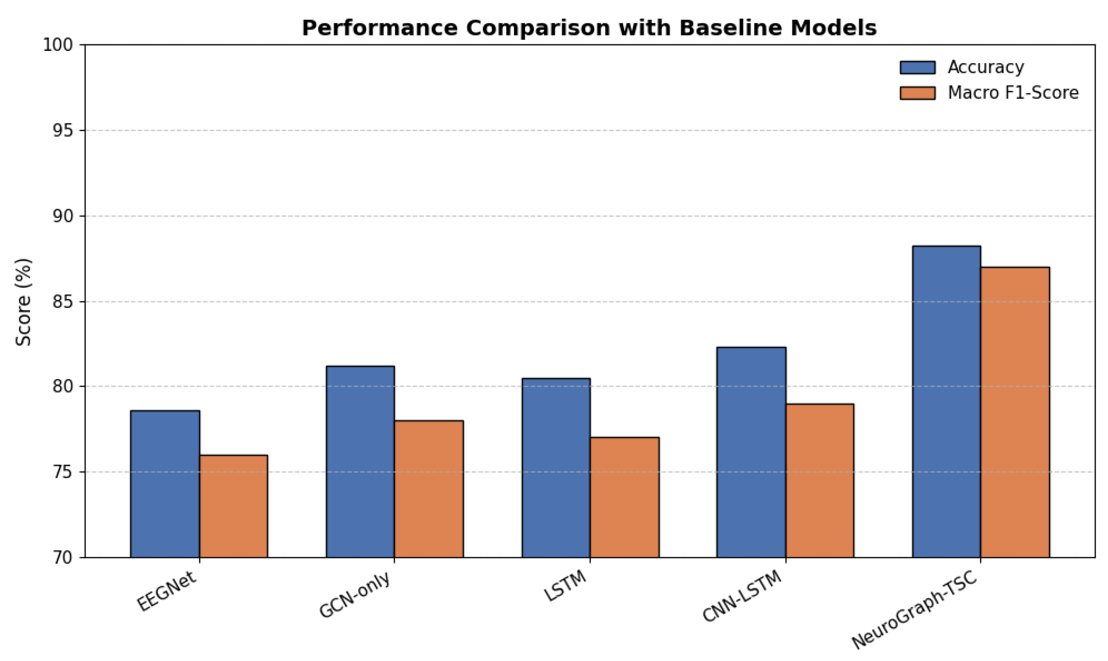
To further contextualize the performance of NeuroGraph-TSC, we benchmarked it against a series of state-of-the-art baseline models commonly used in EEG decoding tasks. These included EEGNet (a compact CNN tailored for EEG), GCN-only (without spectral or dynamic constraints), LSTM (temporal modeling), and CNN-LSTM (joint spatial-temporal modeling). As shown in Table 4, our model outperformed all baselines by a considerable margin, achieving 88.2% accuracy and 0.87 macro F1-score. The improvements are attributable to the synergistic integration of graph-based spatial modeling, temporal context via neural mass constraints, and biologically grounded regularization.
Figure 8.
Grouped bar chart comparing accuracy and F1-scores across all models.
In summary, the empirical validation of NeuroGraph-TSC underscores its effectiveness as both a performant and interpretable model for EEG-based cognitive state classification. Its superior predictive accuracy, coupled with neurophysiological congruence, highlights the potential of biologically guided graph neural networks for advancing brain-computer interface applications.
7. Conclusions and Future Directions
In this study, we proposed NeuroGraph-TSC, a neuro-inspired temporal-spatial classifier for EEG-based cognitive state prediction, specifically targeting the task of stress level classification. The model leverages a graph-based spatial representation of EEG electrode configurations, incorporating physiologically meaningful connectivity through either scalp-geometric distances or data-driven functional edge weights. Temporal dependencies are modeled using a recurrent LSTM encoder that captures multiscale neural dynamics, while a neural mass model regularizer introduces biophysical constraints aligned with established computational neuroscience models such as the Jansen–Rit framework.
The proposed architecture is further guided by a neuroscience-informed composite loss function that not only optimizes classification performance but also enforces realistic oscillatory behavior within the and frequency bands, penalizing deviations from known structural and functional brain patterns. Evaluated on the SAM-40 raw EEG dataset, NeuroGraph-TSC demonstrated superior predictive performance across multiple stress levels and maintained a high degree of interpretability through targeted band-specific analyses and ablation studies.
The integration of domain-specific neurophysiological priors into deep learning offers a compelling avenue for enhancing both the performance and interpretability of EEG-based classifiers. Our results underscore the value of hybrid architectures that couple data-driven learning with neuroscientific constraints, particularly in contexts requiring physiological plausibility and robustness across subjects.
Despite its promising performance, several avenues remain for future research. First, the current model assumes static graph connectivity, which may not fully capture dynamic brain network reconfigurations associated with evolving cognitive states. Incorporating adaptive or time-varying graphs could further enhance model flexibility. Second, while the Jansen–Rit model provides a foundational dynamical constraint, other neural mass or neural field models may offer complementary or more granular physiological insights. Third, extending the model to support multimodal integration, e.g., fNIRS, ECG, or EDA signals, could yield richer representations of affective and cognitive states. Finally, rigorous validation across diverse datasets and populations is necessary to assess the generalizability of the approach for real-world applications such as mental health monitoring, brain–computer interfaces, and cognitive workload assessment.
In conclusion, NeuroGraph-TSC establishes a principled framework for bridging computational neuroscience and machine learning in the domain of EEG-based cognitive state decoding. It opens new opportunities for interpretable and biologically informed neural signal analysis in both foundational research and applied domains.
References
- Calvo, R.A.; D’Mello, S.K. Affective computing and intelligent interaction. IEEE Transactions on Affective Computing 2010, 1, 18–21. [Google Scholar] [CrossRef]
- Fairclough, S.H. Fundamentals of physiological computing. Interacting with Computers 2009, 21, 133–145. [Google Scholar] [CrossRef]
- Acharya, S.; et al. A systematic review of EEG-based mental stress quantification. Computer Methods and Programs in Biomedicine 2025. [Google Scholar] [CrossRef]
- Badri, Y.; et al. A review on evaluating mental stress by deep learning using EEG signals. Soft Computing 2024. [Google Scholar] [CrossRef]
- Niedermeyer, E.; Lopes da Silva, F.H. Electroencephalography: Basic Principles, Clinical Applications, and Related Fields; Lippincott Williams & Wilkins, 2005.
- Belhadi, A.; et al. Enhanced visibility graph and power spectral density features for robust EEG classification. Frontiers in Neuroscience 2025, 19, 1520003. [Google Scholar] [CrossRef] [PubMed]
- Liu, Z.; et al. EEGMind-Transformer: Leveraging deep learning for robust EEG analysis in mental state recognition. Neuroinformatics 2025. [Google Scholar] [CrossRef]
- Lotte, F.; Congedo, M.; Lécuyer, A.; Lamarche, F.; Arnaldi, B. A review of classification algorithms for EEG-based brain–computer interfaces. Journal of neural engineering 2007, 4, R1. [Google Scholar] [CrossRef] [PubMed]
- Jin, K.; Rubio-Solis, A.; Naik, R.; Leff, D.; Kinross, J.; Mylonas, G. Human-Centric Cognitive State Recognition Using Physiological Signals: A Systematic Review of Machine Learning Strategies Across Application Domains. Sensors 2025, 25, 4207. [Google Scholar] [CrossRef] [PubMed]
- Subasi, A. EEG signal classification using wavelet feature extraction and a mixture of expert model. Computer methods and programs in biomedicine 2005, 78, 113–123. [Google Scholar] [CrossRef]
- Díaz-Montiel, A.; et al. Optimal Graph Representations and Neural Networks for EEG Seizure and Phase Classification. Scientific Reports 2025, 15, 1125. [Google Scholar] [CrossRef]
- Kotoge, R.; et al. EvoBrain: Dynamic Multi-Channel EEG Graph Modeling for Time-Adaptive Seizure Prediction. In Proceedings of the International Conference on Learning Representations (ICLR); 2025. [Google Scholar]
- Roy, Y.; Banville, H.; Albuquerque, I.; Gramfort, A.; Falk, T.H.; Faubert, J. Deep learning-based electroencephalography analysis: a systematic review. Journal of Neural Engineering 2019, 16, 051001. [Google Scholar] [CrossRef]
- Schirrmeister, R.T.; Springenberg, J.T.; Fiederer, L.D.J.; Glasstetter, M.; Eggensperger, K.; Tangermann, M.; Hutter, F.; Burgard, W.; Ball, T. Deep learning with convolutional neural networks for EEG decoding and visualization. Human brain mapping 2017, 38, 5391–5420. [Google Scholar] [CrossRef]
- Li, C.; Zhou, X.; et al. Graph Neural Networks in EEG-based Emotion Recognition: A Survey. IEEE Transactions on Affective Computing 2024. [Google Scholar] [CrossRef]
- Delorme, A.; Makeig, S. EEGLAB: an open source toolbox for analysis of single-trial EEG dynamics including independent component analysis. Journal of neuroscience methods 2004, 134, 9–21. [Google Scholar] [CrossRef] [PubMed]
- Wang, L.; Suzumura, T.; Kanezashi, H. Graph-Enhanced EEG Foundation Model: Large-Scale Pretraining with Masked Autoencoders for Brain Signal Analysis. arXiv preprint arXiv:2411.19507 2024.
- Buzsáki, G. Rhythms of the brain; Oxford University Press, 2006.
- Jansen, B.H.; Rit, V.G. Electroencephalogram and visual evoked potential generation in a mathematical model of coupled cortical columns. Biological Cybernetics 1995, 73, 357–366. [Google Scholar] [CrossRef] [PubMed]
- Ghosh, R.; Deb, N.; Sengupta, K.; Phukan, A.; Choudhury, N.; Kashyap, S.; Phadikar, S.; Saha, R.; Das, P.; Sinha, N.; et al. SAM 40: Dataset of 40 subject EEG recordings to monitor the induced-stress while performing Stroop color-word test, arithmetic task, and mirror image recognition task. Data in Brief 2022, 40, 107772. [Google Scholar] [CrossRef]
- Al-Shargie, F.; Tang, T.B.; Kiguchi, M. Mental stress assessment using simultaneous measurement of EEG and fNIRS. Biomedical optics express 2017, 8, 5318–5339. [Google Scholar] [CrossRef] [PubMed]
- Subhani, A.R.; Mumtaz, W.; Kamel, N.; Saad, M.N.; Ali, S.S. Machine learning framework for the detection of mental stress at multiple levels. IEEE Access 2017, 5, 13545–13556. [Google Scholar] [CrossRef]
- Hosseini, S.A.; Khalilzadeh, M.A. Emotional stress recognition system using EEG and fuzzy logic. Journal of Medical Signals and Sensors 2010, 1, 23–30. [Google Scholar]
- Bashivan, P.; Rish, I.; Yeasin, M.; Codella, N. Learning representations from EEG with deep recurrent-convolutional neural networks. arXiv preprint arXiv:1511.06448 2015.
- Lawhern, V.J.; Solon, A.J.; Waytowich, N.R.; Gordon, S.M.; Hung, C.P.; Lance, B.J. EEGNet: A compact convolutional neural network for EEG-based brain–computer interfaces. Journal of Neural Engineering 2018, 15, 056013. [Google Scholar] [CrossRef] [PubMed]
- Tripathi, S.; Acharya, S.; Sharma, R.D.; Mittal, S.; Bhattacharya, S. Using deep and convolutional neural networks for accurate emotion classification on DEAP dataset. In Proceedings of the Proceedings of the AAAI Conference on Artificial Intelligence, 2017, Vol. 31.
- Song, T.; Zheng, W.; Song, P.; Cui, Z.; Zhang, X. EEG emotion recognition using dynamical graph convolutional neural networks. IEEE Transactions on Affective Computing 2018, 11, 532–541. [Google Scholar] [CrossRef]
- Yu, T.; Xiao, J.; Zhang, Y.; Gu, Z.; Li, Y. Graph convolutional networks for EEG-based emotion recognition. IEEE Transactions on Affective Computing 2021, 14, 345–357. [Google Scholar]
- Zhang, Y.; Wang, Y.; Wang, Y.; Jung, T.P. Spatial–temporal attention graph convolutional networks for motor imagery EEG classification. Neurocomputing 2021, 452, 105–115. [Google Scholar]
- Liu, Y.; Zheng, W.; Lu, B.L. Dynamic functional connectivity analysis for depression recognition using EEG-based GNNs. IEEE Transactions on Neural Systems and Rehabilitation Engineering 2021, 29, 1552–1562. [Google Scholar]
- Kietzmann, T.C.; Spoerer, C.J.; Sörensen, L.K.; Cichy, R.M.; Hauk, O.; Kriegeskorte, N. Recurrence is required to capture the representational dynamics of the human visual system. Proceedings of the National Academy of Sciences 2019, 116, 21854–21863. [Google Scholar] [CrossRef] [PubMed]
Figure 1.
Overview of the NeuroGraph-TSC architecture showing spatial graph encoding, temporal sequence modeling, and neural mass model-based regularization.
Figure 1.
Overview of the NeuroGraph-TSC architecture showing spatial graph encoding, temporal sequence modeling, and neural mass model-based regularization.
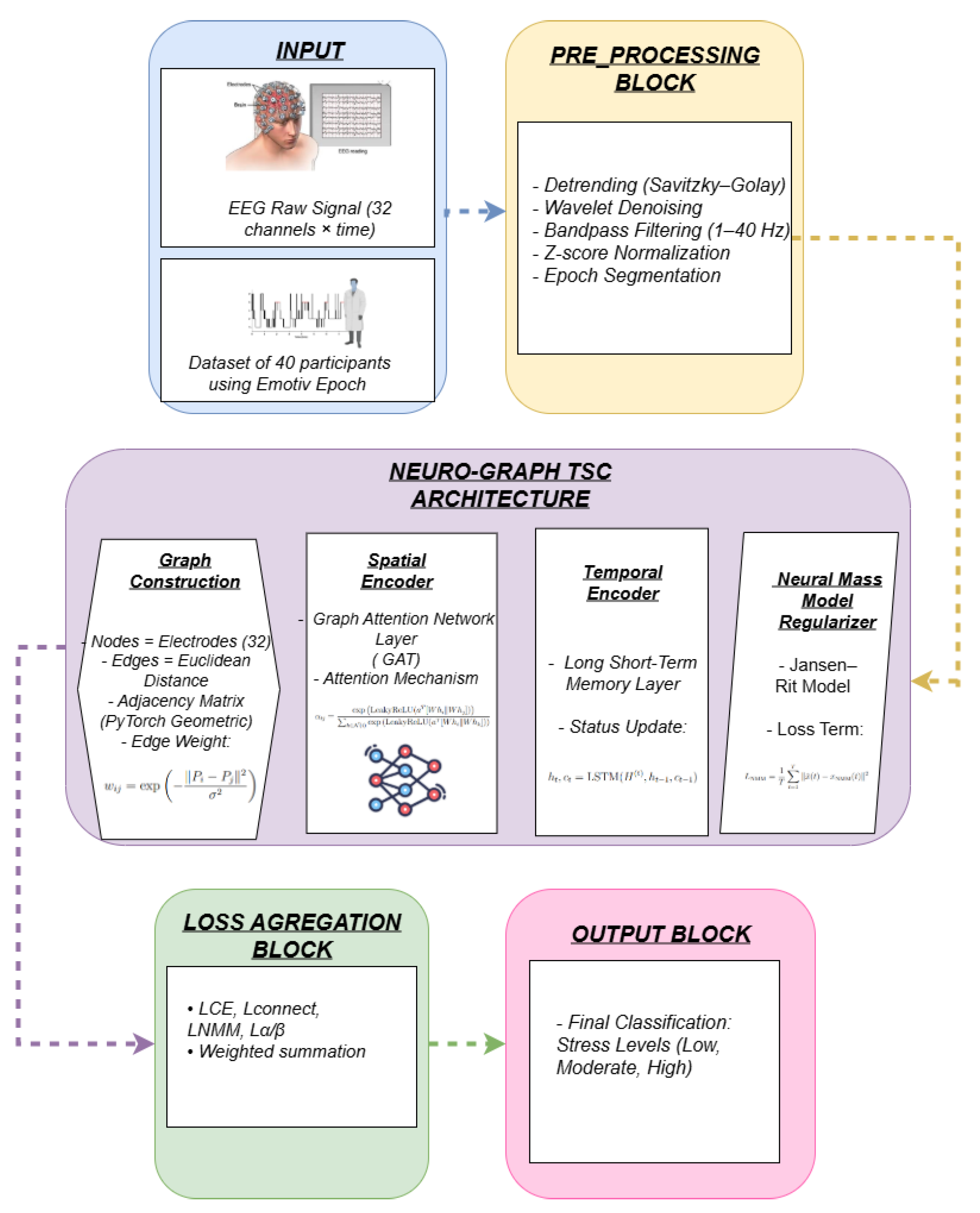
Figure 2.
Line plots showing training and validation accuracy and loss across epochs.
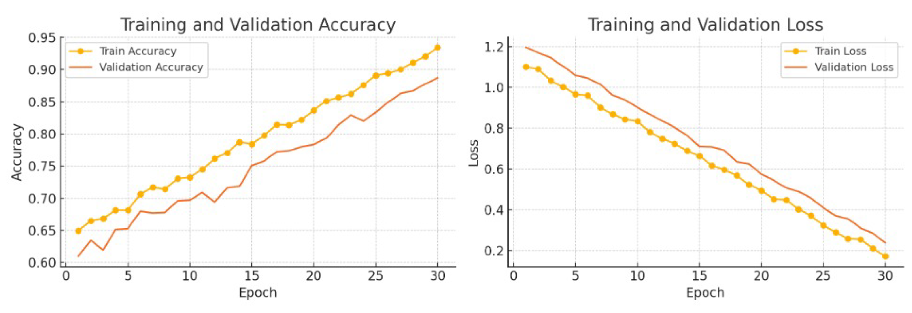
Figure 4.
Bar chart comparing per-class F1-scores.
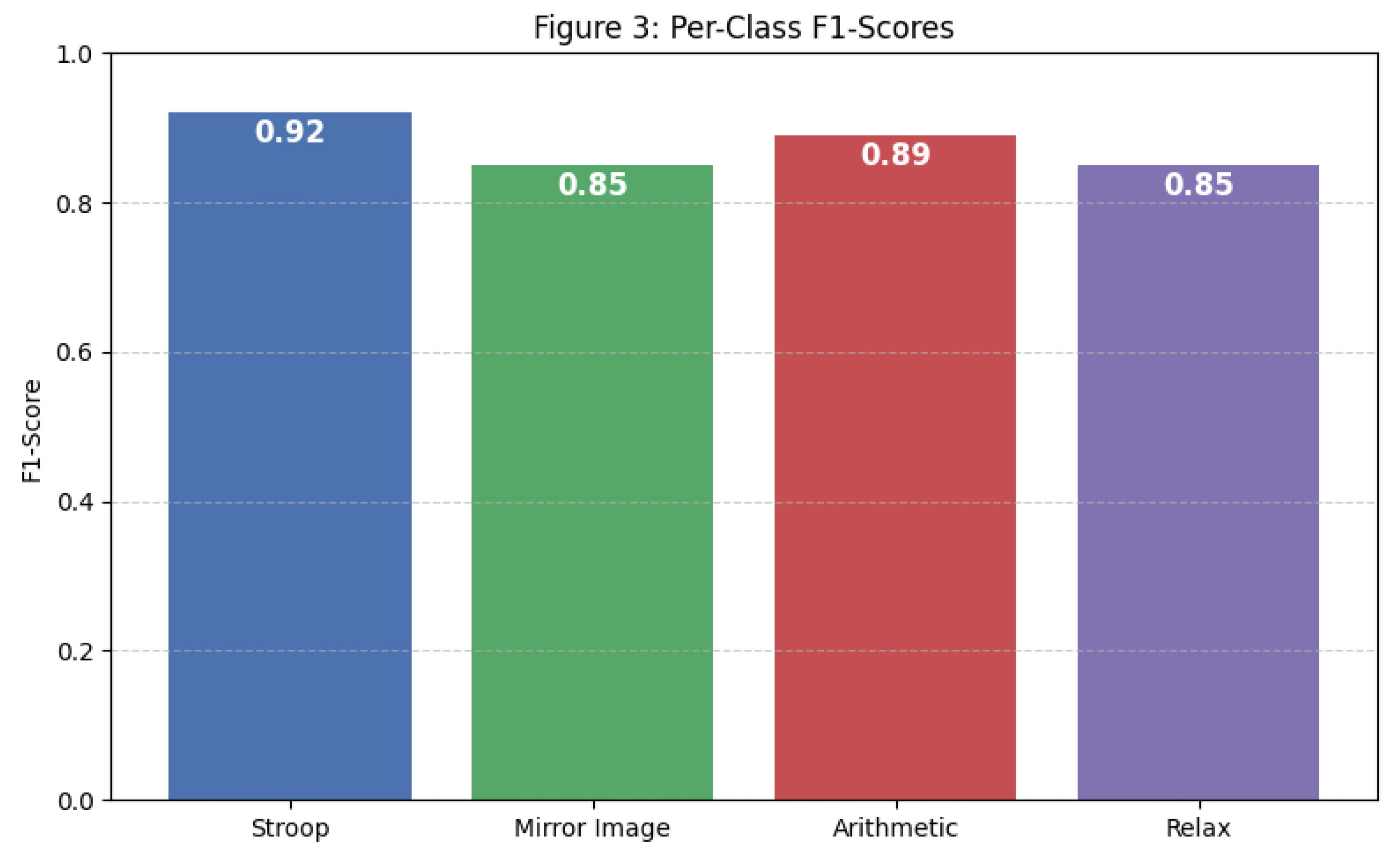
Figure 5.
Attention heatmaps across the scalp for each cognitive task.
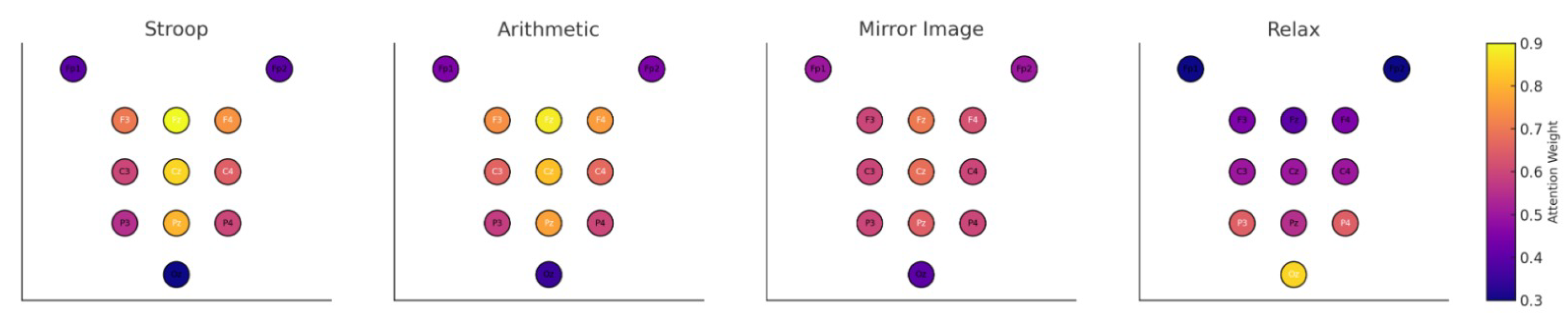
Table 2.
Precision, Recall, and F1-Scores by Class
| Class | Precision | Recall | F1-Score |
|---|---|---|---|
| Stroop | 0.92 | 0.91 | 0.92 |
| Mirror Image | 0.86 | 0.83 | 0.85 |
| Arithmetic | 0.88 | 0.90 | 0.89 |
| Relax | 0.84 | 0.85 | 0.85 |
| Macro Average | 0.88 | 0.87 | 0.87 |
Table 3.
Ablation Study: F1-Scores Under Different Model Variants
| Model Variant | Macro F1-Score | Drop () |
|---|---|---|
| Full NeuroGraph-TSC | 0.87 | – |
| w/o | 0.82 | –5.1% |
| w/o | 0.84 | –3.2% |
| w/o | 0.85 | –2.7% |
Table 4.
Performance Comparison with Baseline Models
| Model | Accuracy | Macro F1-Score |
|---|---|---|
| EEGNet | 78.6% | 0.76 |
| GCN-only | 81.2% | 0.78 |
| LSTM | 80.5% | 0.77 |
| CNN-LSTM | 82.3% | 0.79 |
| NeuroGraph-TSC (Ours) | 88.2% | 0.87 |
Disclaimer/Publisher’s Note: The statements, opinions and data contained in all publications are solely those of the individual author(s) and contributor(s) and not of MDPI and/or the editor(s). MDPI and/or the editor(s) disclaim responsibility for any injury to people or property resulting from any ideas, methods, instructions or products referred to in the content. |
© 2025 by the authors. Licensee MDPI, Basel, Switzerland. This article is an open access article distributed under the terms and conditions of the Creative Commons Attribution (CC BY) license (http://creativecommons.org/licenses/by/4.0/).
Copyright: This open access article is published under a Creative Commons CC BY 4.0 license, which permit the free download, distribution, and reuse, provided that the author and preprint are cited in any reuse.


