Machine Learning Methods for Classifying Gas Discharge Images of Liquid Solutions

1. Introduction

The contemporary enhancement in computational capabilities facilitates the utilisation of mathematical models across diverse disciplines, encompassing fluid analysis. Conventional techniques for fluid analysis, including mass spectrometry, chromatography, spectrophotometry, photometry, polarography, and potentiometry, are employed in both manual and automated modes with the assistance of machine learning methodologies [1,2,3,4]. These approaches necessitate the execution of measurements and analysis in a laboratory setting, utilising specialised equipment. The operation of such equipment necessitates a particular set of competencies and consumables, whilst the analytical process itself is s time-consuming.

The behavior of water in the presence of magnetic fields has been a subject of scientific interest for a considerable period. A significant challenge in this field pertains to the complexity of evaluating the impact of magnetic fields on water. Fortunately, in the last few years, several studies have demonstrated the influence of weak and super-weak constant and variable magnetic fields on aqueous systems that do not contain admixtures sensitive to magnetic fields. In the latest review [5] presented conceptual ideas and demonstrated a wide range of practical applications in medicine [6,7], agriculture [8,9], wastewater treatment [10], and human health parameters [11]. Therefore, a large amount of experimental data has been collected, proving that weak and super-weak magnetic fields have reproducible effects on water solutions. These effects are most prominent when static and variable magnetic fields are used simultaneously. On the other hand, reliable data recently suggested that magnetic and electromagnetic fields could significantly influence the properties of highly diluted aqueous solutions [12].

The utilisation of machine learning (ML) methodologies within the domain of mass spectrometry (MS) has been a subject of considerable research interest [1]. It is evident that MS is confronted with challenges at each stage of the process, from the initial collection of data to its subsequent interpretation. To elaborate, the data complexity (for example, the dimensionality of the feature space) poses significant challenges. Machine learning provides tools to address these issues; however, further development is required in the areas of standardisation and explainability. Furthermore, the study [2] dedicated to imaging mass spectrometry (IMS) discusses challenges in interpretability (relating machine learning (ML) results to physicochemical patterns) and the high dimensionality of the feature space.

In order to address the challenges posed by data complexity, the employment of unsupervised machine learning algorithms has become a prevalent approach. For instance, the review article [3] focuses on the use of unsupervised ML methods for exploratory data analysis in imaging mass spectrometry (IMS). The text is organised around three main directions: factorization, clustering, and manifold learning. Unsupervised methods are well-suited for the analysis of IMS data due to the fact that IMS produces large and complex datasets containing spatial and spectral information.

The employment of screening instruments such as online UV-Vis spectrophotometers facilitates real-time monitoring of drinking water quality. However, these instruments necessitate configuration and calibration, and their maintenance requires expertise in spectroscopy [4]. The article observes that elevated turbidity or organic content necessitates regular recalibration (due to the distortion of spectra caused by high turbidity or concentrations of organic matter).

The utilisation of gas discharge visualization (GDV) methodologies [13] has been demonstrated to facilitate the circumvention of the aforementioned issues. For instance, the analysis time is approximately one minute, and no special laboratory conditions or consumables are required. The output of GDV analysis is an image, and the complexity of the data is dependent on the specific task and the processing methods employed [13,14,15].

Machine learning has also been employed in the domain of gas discharge visualization, with numerous studies attaining substantial outcomes.

In study [16], a mathematical model of GDV parameters was developed. This model utilised glow intensity and average area of the GDV images as features, and a health deviation index as the target label, with this index being based on questionnaires. The k-means algorithm was utilised to categorise the 20 subjects into distinct subclasses. Subsequently, the distances between each sample and an “ideal health state” (defined in a phase space) were calculated. A linear relationship was established between the distance and the health deviation index.

In the study [17], a GDV method was developed for the analysis of biological objects in the liquid phase. The method was primarily focused on the diagnosis of thyroid diseases, with the magnesium concentration in oral fluid being measured as a key indicator. Utilising the proposed mathematical model, the authors established a correlation between GDV streamer characteristics and the physicochemical properties of the fluid and voltage parameters. The streamer characteristics were determined using classical computer vision. The dataset under consideration consisted of 60 objects. The feasibility of detecting salt ions such as NaCl, MgSO4, KCl, CaCl2, FeSO4, or their complexes in a single liquid-phase biological object (LPBO) was demonstrated.

In the study [18], features extracted from GDV images were employed to train an SVM (Support Vector Machine) machine learning model. The total number of objects involved in the study was 85.

A number of studies [19,20] have explored the possibility of disease classification using machine learning algorithms based on features extracted from GDV. The target labels were extracted from ultrasound diagnostic reports. The dataset under consideration consisted of approximately 170 objects.

Article [21] posits a methodology for the identification of diseases through the utilisation of GDV. Following an initial series of preprocessing steps that utilise classical computer vision techniques, a segmentation approach is then employed that is based on color intensity. This segmentation process is utilised for the purpose of identifying regions of high energy. Subsequently, feature extraction is conducted utilising Particle Swarm Optimization (PSO), followed by disease classification employing Bayesian Gaussian Mixture Models (BGMMs), which are models based on bivariate Gaussian mixture models.

2. Analysis of Gdv Images for Classification of Liquid Solutions

A considerable challenge faced by researchers and practitioners working with data is the limited number of class instances in datasets. In the specific case of image-related tasks, such constraints can have a substantial detrimental effect on the training process of machine learning models. A viable approach to address this issue is the application of classical machine learning methods. In this context, it is important to note that object features can be extracted using traditional engineering techniques such as classical computer vision. The efficacy of these methods is twofold: firstly, they enhance the quality of feature extraction, and secondly, they improve the human interpretability of model results.

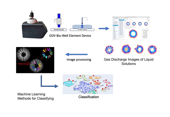
The acquisition and analysis of GDV images is facilitated by the utilisation of the standard Bio-Well Element device. A volume of the test liquid, predetermined by the operator, is then applied to the device’s electrode. The subject is exposed to an electromagnetic field, which results in the emission of a glow that is then captured by the GDV camera. The resulting image is illustrated in Figure 1.

Figure 1. Example of a GDV image of a water droplet.

Figure 1. Example of a GDV image of a water droplet.

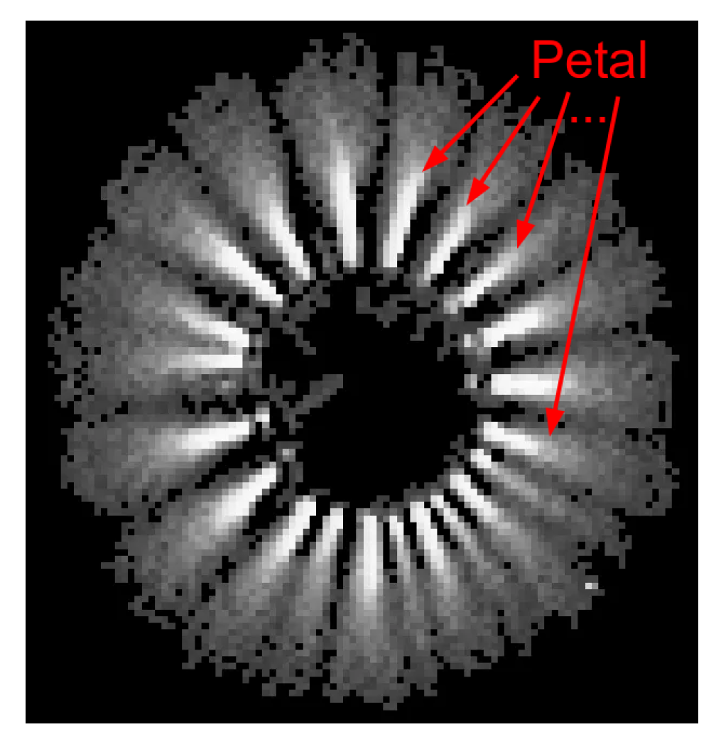
The images in the GDV manifest as “petals” surrounding the droplet (petal in Figure 1). The configuration of these particles, including their shape, number, and positioning, is contingent upon the nature of the liquid under analysis. Given the observed similarity in shape between the GDV images, it is rational to employ computer vision methodologies for their analysis. The resulting image can thus be represented as an intensity matrix, where the number of rows and columns corresponds to the height and width of the image, respectively. The matrix in question is denoted by A (1), and its number of rows and columns are designated as n and m, respectively:

$$A=\left(\begin{array}{cccc}{a}_{11}& a_{12}& \dots & a_{1m}\\ a_{21}& a_{22}& \dots & a_{2m}\\ ⋮& ⋮& \ddots & ⋮\\ a_{n1}& a_{n2}& \dots & a_{nm}\end{array}\right).$$

(1)

Each element of matrix (1), $a_{ij}$, represents intensity. With this intensity matrix, it is possible to calculate the average brightness ${\mu }_g$ (2), the standard deviation of brightness ${\sigma }_g$ (3), and the difference between the peak and minimum intensity ${\Delta }_g$ (4).

$${\mu }_g={\displaystyle \frac{1}{n·m}}\sum _{i=1}^n\sum _{j=1}^m{a}_{ij}.$$

(2)

$${\sigma }_g=\sqrt{{\displaystyle \frac{1}{n·m}}\sum _{i=1}^n\sum _{j=1}^m{(a_{ij}-{\mu }_g)}^2}.$$

(3)

$${\Delta }_g=max\left(a_{ij}\right)-min\left(a_{ij}\right).$$

(4)

These estimates allow for an assessment of general intensity characteristics. However, for a more detailed analysis of the image and the application of morphological methods, it is necessary to remove the “noise component” using thresholding or simplest tone correction (5).

$$f\left(x\right)=\left\{\begin{array}{cc}0\hfill & \mathrm{if}x<L\hfill \\ x\hfill & \mathrm{if}L\le x\le H\hfill \\ 0\hfill & \mathrm{if}x>H\hfill \end{array}\right.,$$

(5)

where $x=A(i,j)$ – the original pixel intensity.

$f\left(x\right)$ – adjusted intensity.

L and H are the calibration parameters of the device.

Representing the image as a matrix (1) also enables the calculation of the center of mass $(x_c,y_c)$ as follows:

$$x_c={\displaystyle \frac{1}{M}}\sum _{i=1}^n\sum _{j=1}^{m}j·a_{ij};y_c={\displaystyle \frac{1}{M}}\sum _{i=1}^n\sum _{j=1}^{m}i·a_{ij},$$

(6)

where M is the "mass" of the image (7).

$$M=\sum _{i=1}^m\sum _{j=1}^{n}A\left[i\right]\left[j\right].$$

(7)

Utilising equations (6) and (7), it is feasible to estimate the locations of the centers of the inscribed and circumscribed circles, the relative positions of these centers (mass center, inscribed circle center, circumscribed circle center), as well as the radii of such circles. These parameters are features that have been extracted from the GDV image. In order to delineate the petals’ boundaries with greater clarity, a morphological operation known as opening (sequential erosion and dilation) is performed with a kernel $k_m$ (8).

$$k_m=\left(\begin{array}{ccc}0& 1& 0\\ 1& 1& 1\\ 0& 1& 0\end{array}\right).$$

(8)

The selection of (8) is predicated on the premise that n and m are ordinarily modest values, and the shortest distance between petals is ordinarily merely a small number of elements of matrix A (1). Subsequently, the erosion (9) and dilation (10) operations are performed in sequence (morphological opening).

$$A_{er}(i,j)=min\{A(i+k,j+l)\mid (k,l)\in k_m\},$$

(9)

$$A_{open}(i,j)=max\{A_{er}(i+k,j+l)\mid (k,l)\in k_m\}.$$

(10)

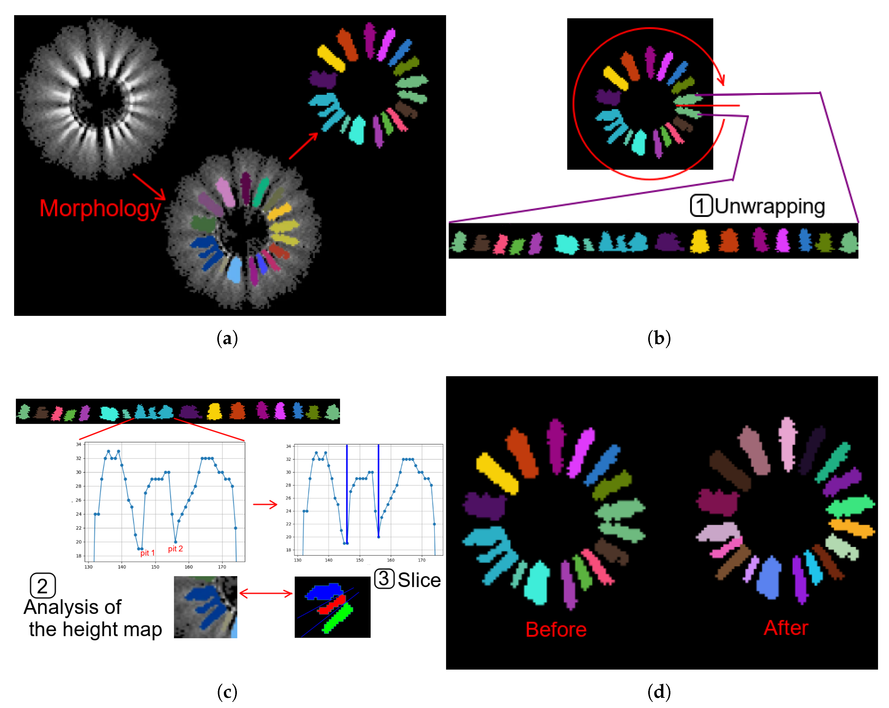
After the opening operation, a slicing operation of the unwrapping is performed. This step is necessary to cut the petals correctly, as even after the opening operation, there may still be “stuck” petals. To address this issue, additional image processing is carried out in three steps (see Figure 2):

• Unwrapping;
• Analysis of the height map;
• Slicing.

Figure 2. Example of performing petal refinement operations: (a) Example of morphology result. (b) Example of performing a unwrapping. (c) Example of analysis of the height map and slicing. (d) Comparison before and after.

Figure 2. Example of performing petal refinement operations: (a) Example of morphology result. (b) Example of performing a unwrapping. (c) Example of analysis of the height map and slicing. (d) Comparison before and after.

Following the implementation of the aforementioned transformation, the identification of petal components can be accomplished through the utilisation of connected component analysis. The ascertainment of the locations of the aforementioned petals enables the establishment of the guidelines that are directed towards the centre of mass of each individual petal. The vector $d_i$ of the guiding line from the center of mass of the entire GDV image to the center of mass of the petal is denoted by the formula (11), and the vector of lines is denoted by the formula (12).

$$d_i=\left[\begin{array}{c}{x}_i-x_c\\ y_i-y_c\end{array}\right],$$

(11)

$$V_d=\left\{\overrightarrow{d_1},\overrightarrow{d_2},\dots ,\overrightarrow{d_n}\right\}=\left\{\left[\begin{array}{c}{x}_1-x_c\\ y_1-y_c\end{array}\right],\left[\begin{array}{c}{x}_2-x_c\\ y_2-y_c\end{array}\right],\dots ,\left[\begin{array}{c}{x}_n-x_c\\ y_n-y_c\end{array}\right]\right\}.$$

(12)

We calculate the angles ${\theta }_i$ between the lines (13), which also is features $\mathrm{\Theta }=\left\{{\theta }_1,{\theta }_2,\dots ,{\theta }_n\right\}$, identifying the class of the GDV image.

$${\theta }_i=arccos\left({\displaystyle \frac{x_i-x_c}{\sqrt{{(x_i-x_c)}^2+{(y_i-y_c)}^2}}}\right).$$

(13)

Let $V_p$ be the vector containing the coordinate vectors of the petals. It is defined by the formulas (14) and (15). The vector of projections of the pixels of the petals onto the corresponding guides is defined by the formula (16).

$$\overrightarrow{V_p}=\{\overrightarrow{V_{p1}},\overrightarrow{V_{p2}},\dots \},$$

(14)

$$\overrightarrow{V_{pi}}=(x_{pi1},y_{pi1}),(x_{pi2},y_{pi2}),\dots ,(x_{pin},y_{pin}),$$

(15)

$$P=\{{\mathrm{proj}}_{\overrightarrow{d_1}}\overrightarrow{V_{p1}},{\mathrm{proj}}_{\overrightarrow{d_2}}\overrightarrow{V_{p2}},\dots \},$$

(16)

where ${\mathrm{proj}}_{\overrightarrow{d_i}}\overrightarrow{V_{pi}}$ is a vector in which each element is a petal point projected onto the guiding line $d_i$. Using this vector, it is possible to determine the length of each petal by formula (17).

$${\mathrm{len}}_i=max\left({\mathrm{proj}}_{\overrightarrow{d_i}}\overrightarrow{V_{pi}}\right)-min\left({\mathrm{proj}}_{\overrightarrow{d_i}}\overrightarrow{V_{pi}}\right).$$

(17)

In the event of the projection being made onto a line perpendicular to $d_i$, the width can also be computed. It is evident that both length and width are features of the GDV image.

Another feature of the characteristics of GDV images is the presence of structuredness ($S_{LF}$) and noisiness ($S_{HF}$) (see formulas (18) and (19)). The determination of these parameters is achieved through the utilisation of spectral transformation techniques, with the Discrete Cosine Transform serving as a representative example (see formula (20)).

$$C(u,v)={\displaystyle \frac{2}{\sqrt{nm}}}\sum _{x=0}^{n-1}\sum _{y=0}^{m-1}A(x,y)cos\left({\displaystyle \frac{(2x+1)u\pi }{2n}}\right)cos\left({\displaystyle \frac{(2y+1)v\pi }{2m}}\right),$$

(18)

$$S_{LF}=\sum _{(u,v)\in LF}{\left|C(u,v)\right|}^2,$$

(19)

$$S_{HF}=\sum _{(u,v)\in HF}{\left|C(u,v)\right|}^2.$$

(20)

In this text, the term “low-frequency coefficient region” is abbreviated to “LF”, and the term “high-frequency coefficient region” is abbreviated to “HF”.

Utilising the aforementioned features and their derivatives, it is feasible to formulate a vector of numerical values, wherein each element corresponds to a numerical expression of a qualitative feature. This vector serves as the numerical representation of the GDV image.

3. Results

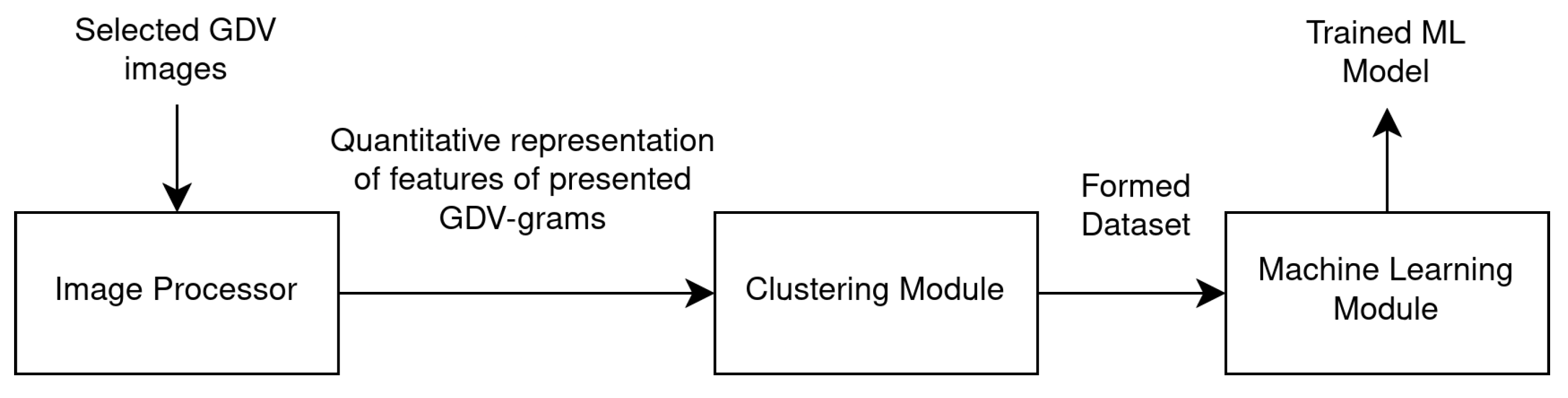
The formation of a set of features that serve to identify GDV images was achieved through the development of a processing pipeline. This pipeline involves the utilisation of an image processor, which is employed to extract quantitative features from the image. These features are then forwarded to the clustering module, which enables data visualisation, provides an initial understanding of the structure of the GDV images used, and generates a dataset that is then passed to the machine learning module (see Figure 3).

Figure 3. Data flow between modules.

Figure 3. Data flow between modules.

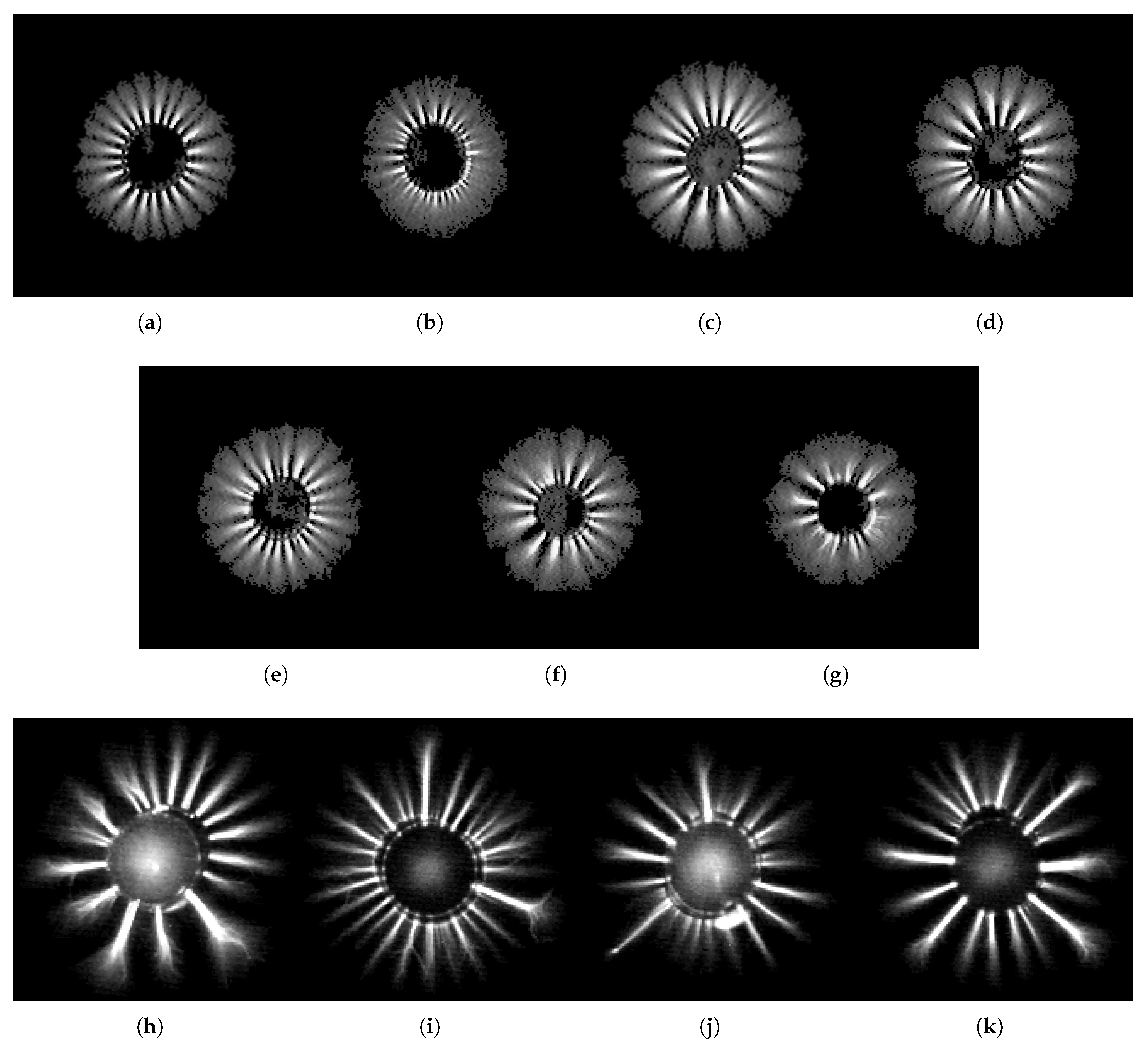
In order to evaluate the applicability of the method, a dataset of GDV images was collected (see Table 1 and Figure 4). This dataset represents images of water with various impurities and additives, including distilled water, filtered tap water, water from three different springs, water with added magnesium, water with added salt, and water with added shungite. A sample was obtained from one of the springs and subjected to treatment using a coil that generated an electromagnetic field (EMF).

Table 1. Description of classes.

Class	Description	Number of objects
1	Filtered tap water	10080
2	Distilled water	9040
3	Spring 3	105
4	Spring 3, EMF-treated	1513
5	Spring 1	60
6	Spring 2	60
7	Tea with sugar	15
8	Water with magnesium additive	10
9	Water with magnesium additive, exposed to UV light for 2–5 minutes	20
10	Water with salt additive	30
11	Water with shungite additive	20

Table 1. Description of classes.

Class	Description	Number of objects
1	Filtered tap water	10080
2	Distilled water	9040
3	Spring 3	105
4	Spring 3, EMF-treated	1513
5	Spring 1	60
6	Spring 2	60
7	Tea with sugar	15
8	Water with magnesium additive	10
9	Water with magnesium additive, exposed to UV light for 2–5 minutes	20
10	Water with salt additive	30
11	Water with shungite additive	20

Figure 4. Class examples: (a) Class 1 (filtered tap water). (b) Class 2 (distilled water). (c) Class 3 (spring 3). (d) Class 4 (spring 3 + EMF). (e) Class 5 (spring 1). (f) Class 6 (spring 2). (g) Class 7 (tea with sugar). (h) Class 8 (magnesium). (i) Class 9 (magnesium + UV). (j) Class 10 (salt). (k) Class 11 (shungite).

Figure 4. Class examples: (a) Class 1 (filtered tap water). (b) Class 2 (distilled water). (c) Class 3 (spring 3). (d) Class 4 (spring 3 + EMF). (e) Class 5 (spring 1). (f) Class 6 (spring 2). (g) Class 7 (tea with sugar). (h) Class 8 (magnesium). (i) Class 9 (magnesium + UV). (j) Class 10 (salt). (k) Class 11 (shungite).

The selected images are passed to the image processor module (see Figure 3), which extracts approximately 57 features as a feature space. In particular, the following key features are extracted:

• number of pixels with and without noise, statistical characteristics of pixel distributions;
• mean intensity and standard deviation of intensity;
• radii of circles;
• difference between the center of mass and the centers of the circles;
• characteristics of "petals": number, size, positioning, etc.;
• characteristics of noisiness;
• characteristics from spectral transforms.

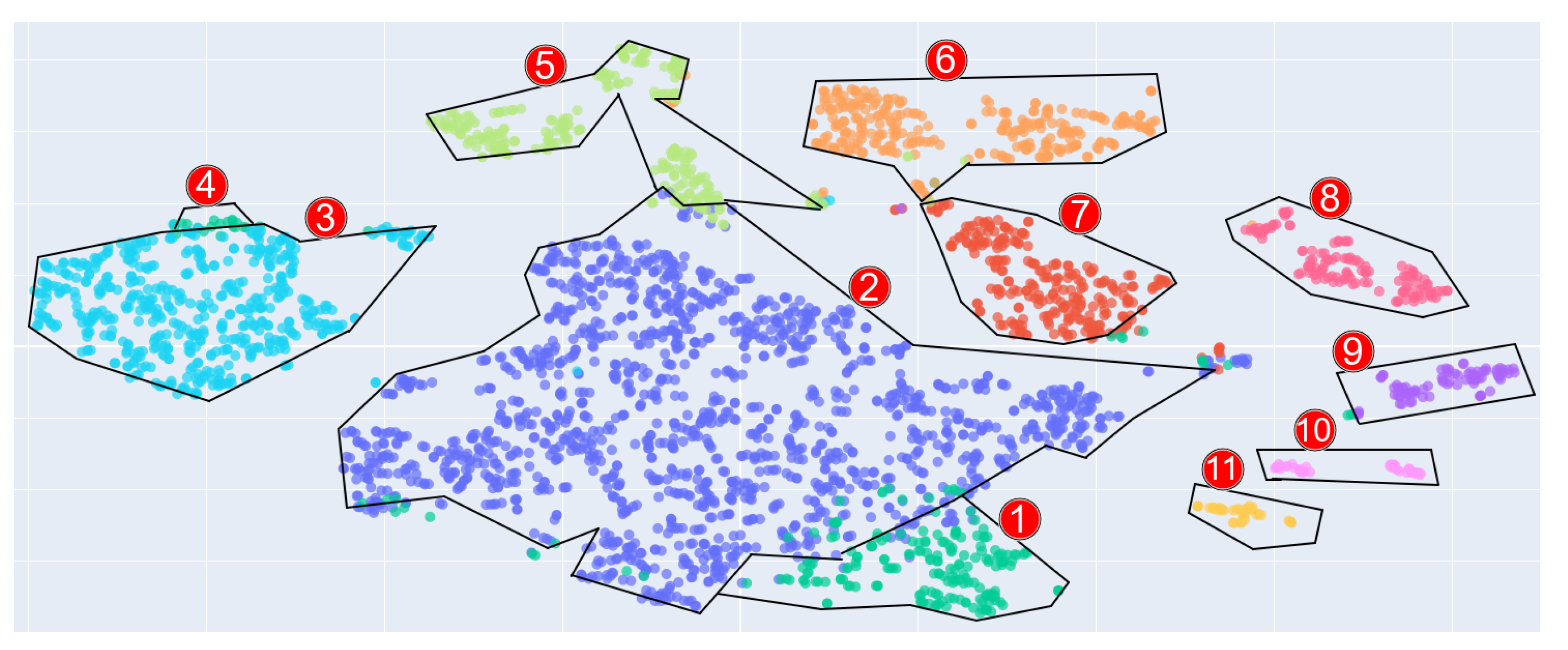
The resulting feature space of a GDV image allows it to be assigned to a particular class. The purpose of the clustering module is to visualise the multidimensional feature space of the GDV images by projecting them onto a 2D plane (see Figure 5). Each point on the plane is representative of a GDV object, colored according to its associated class/cluster. For instance, blue and dark green points (labelled 1 and 2, respectively) represent filtered tap water, turquoise (labelled 3) denotes distilled water, and so on. This approach facilitates exploratory data analysis.

Figure 5. GDV-gram projection in feature space.

Figure 5. GDV-gram projection in feature space.

Following a thorough analysis of the clustering results and subject field, a dataset is compiled in the form of GDV object features and class labels and fed to the machine learning module. The following models are employed: logistic regression (logreg), decision tree (DT), random forest (RF), gradient boosting, support vector machines (SVM), and k-nearest neighbors (KNN).

The dataset was segmented into two distinct components: 80% was allocated to the training set, while the remaining 20% was designated for the test set. The machine learning models were trained on the training dataset and validated on the test dataset. During the training phase, the models were not permitted to access the test dataset objects.

The performance metrics reported hereinafter are calculated using a weighted approach that takes into account the number of objects in each class.

A selection of metrics is presented in Table 2.

Table 2. Model training metrics.

Model	Train dataset		Test dataset
	Metric	Score	Metric	Score
Logreg	accuracy	0.991	accuracy	0.990
	precision	0.991	precision	0.989
	recall	0.991	recall	0.990
	f1	0.991	f1	0.989
Decision Tree	accuracy	0.997	accuracy	0.986
	precision	0.997	precision	0.987
	recall	0.997	recall	0.986
	f1	0.997	f1	0.986
Random forest	accuracy	0.999	accuracy	0.995
	precision	0.999	precision	0.995
	recall	0.999	recall	0.995
	f1	0.999	f1	0.994
XGBoost	accuracy	1.000	accuracy	0.997
	precision	1.000	precision	0.997
	recall	1.000	recall	0.997
	f1	1.000	f1	0.997
SVC	accuracy	0.995	accuracy	0.992
	precision	0.995	precision	0.992
	recall	0.995	recall	0.992
	f1	0.994	f1	0.992
KNN	accuracy	0.996	accuracy	0.995
	precision	0.996	precision	0.995
	recall	0.996	recall	0.995
	f1	0.996	f1	0.995

Table 2. Model training metrics.

Model	Train dataset		Test dataset
	Metric	Score	Metric	Score
Logreg	accuracy	0.991	accuracy	0.990
	precision	0.991	precision	0.989
	recall	0.991	recall	0.990
	f1	0.991	f1	0.989
Decision Tree	accuracy	0.997	accuracy	0.986
	precision	0.997	precision	0.987
	recall	0.997	recall	0.986
	f1	0.997	f1	0.986
Random forest	accuracy	0.999	accuracy	0.995
	precision	0.999	precision	0.995
	recall	0.999	recall	0.995
	f1	0.999	f1	0.994
XGBoost	accuracy	1.000	accuracy	0.997
	precision	1.000	precision	0.997
	recall	1.000	recall	0.997
	f1	1.000	f1	0.997
SVC	accuracy	0.995	accuracy	0.992
	precision	0.995	precision	0.992
	recall	0.995	recall	0.992
	f1	0.994	f1	0.992
KNN	accuracy	0.996	accuracy	0.995
	precision	0.996	precision	0.995
	recall	0.996	recall	0.995
	f1	0.996	f1	0.995

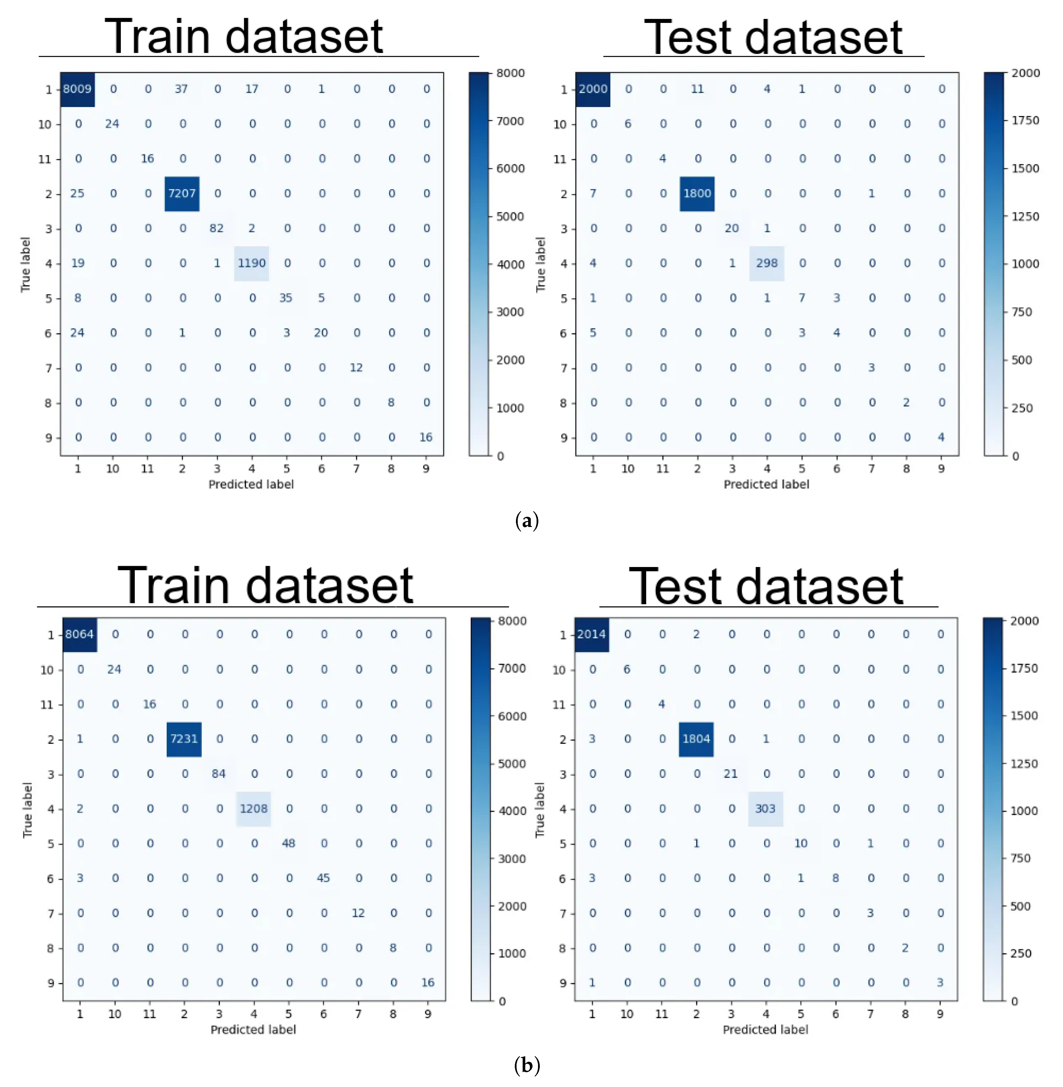
All models except gradient boosting confused classes 1, 5, and 6 (filtered tap, spring 1, and spring 2). Specifically, the confusion matrix for logistic regression is shown in Figure 6 (a). Gradient boosting was able to recognize the mentioned classes with minimal error. Its confusion matrix is presented in Figure 6 (b).

Figure 6. Confusion matrix for train and test datasets: (a) Confusion matrix of logistic regression. (b) Confusion matrix of gradient boosting.

Figure 6. Confusion matrix for train and test datasets: (a) Confusion matrix of logistic regression. (b) Confusion matrix of gradient boosting.

Some of the selected hyperparameters for the models are listed in Table 3.

Table 3. Selected hyperparameters of some models.

Model	Hyperparameter	Value
Logreg	C (inverse of regularization strength)	1.0
Decision Tree	max depth	25
	min samples leaf	3
	min samples split	2
Random forest	estimators num	150
	max depth	25
	min samples leaf	3
	min samples split	2
	max samples	80%
	max features	80%
Gradient boosting	estimators num	100
	max depth	3
	learning rate	0.1
	min child weight	1
	max samples	80%
	max features	80%
SVC	kernel	rbf
KNN	n neighbors	5

Table 3. Selected hyperparameters of some models.

Model	Hyperparameter	Value
Logreg	C (inverse of regularization strength)	1.0
Decision Tree	max depth	25
	min samples leaf	3
	min samples split	2
Random forest	estimators num	150
	max depth	25
	min samples leaf	3
	min samples split	2
	max samples	80%
	max features	80%
Gradient boosting	estimators num	100
	max depth	3
	learning rate	0.1
	min child weight	1
	max samples	80%
	max features	80%
SVC	kernel	rbf
KNN	n neighbors	5

It can be concluded from the results obtained that images of water droplets GDV can be classified using machine learning models. All trained models demonstrate a high degree of confusion between filtered tap water and spring water, with XGBoost being the sole exception. Therefore, on the basis of the given dataset, XGBoost is the most suitable model.

4. Conclusions

In the course of the study, a methodology for the analysis of GDV images through the application of machine learning algorithms was developed. This methodology was employed for the classification of liquid solutions, with the capacity to accurately differentiate between the various types presented. A logical direction for further research is to expand the range of liquid classes under investigation.

References

- Beck, A.G.; Muhoberac, M.; Randolph, C.E.; Beveridge, C.H.; Wijewardhane, P.R.; Kenttamaa, H.I.; Chopra, G. Recent developments in machine learning for mass spectrometry. ACS Measurement Science Au 2024, 4, 233–246. [CrossRef]
- Jetybayeva, A.; Borodinov, N.; Ievlev, A.V.; Haque, M.I.U.; Hinkle, J.; Lamberti, W.A.; Meredith, J.C.; Abmayr, D.; Ovchinnikova, O.S. A review on recent machine learning applications for imaging mass spectrometry studies. Journal of Applied Physics 2023, 133. [CrossRef]
- Verbeeck, N.; Caprioli, R.M.; Van de Plas, R. Unsupervised machine learning for exploratory data analysis in imaging mass spectrometry. Mass spectrometry reviews 2020, 39, 245–291. [CrossRef]
- Shi, Z.; Chow, C.W.; Fabris, R.; Liu, J.; Jin, B. Applications of online UV-Vis spectrophotometer for drinking water quality monitoring and process control: a review. Sensors 2022, 22, 2987. [CrossRef]
- Moussa, M.; Besma, Z.; Hachicha, M. Magnetic water treatment: theory and effects on treated water–a systematic review. Euro-Mediterranean Journal for Environmental Integration 2025, pp. 1–20. [CrossRef]
- Johnson, K.E.; Sanders, J.J.; Gellin, R.G.; Palesch, Y.Y. The effectiveness of a magnetized water oral irrigator (Hydro Fioss®) on plaque, calculus and gingival health. Journal of clinical periodontology 1998, 25, 316–321. [CrossRef]
- Gholizadeh, M.; Arabshahi, H.; Saeidi, M.R.; Mahdavi, B. The effect of magnetic water on growth and quality improvement of poultry. Middle-East Journal of Scientific Research 2008, 3, 140–144.
- Carbonell, M.V.; Martinez, E.; Amaya, J.M. Stimulation of germination in rice (Oryza sativa L.) by a static magnetic field. Electro-and magnetobiology 2000, 19, 121–128. [CrossRef]
- Maheshwari, B.L.; Grewal, H.S. Magnetic treatment of irrigation water: Its effects on vegetable crop yield and water productivity. Agricultural water management 2009, 96, 1229–1236. [CrossRef]
- Moussa, M.; Michot, D.; Hachicha, M. Effect of electromagnetic treatment of treated wastewater on soil and drainage water. Desalination and Water Treatment 2021, 213, 177–189. [CrossRef]
- Hassan, T.M.M.; Almahdi, M.R.; Hafez, Y.H.; El-Khashen, O.A. Effect of using Magnetic Water on Zaraibi Kid’s Growth Performance, Carcass Traits, Blood Metabolites and Immunity. Annals of Agricultural Science, Moshtohor 2024, 62, 87–96. [CrossRef]
- Coey, J.; Cass, S. Magnetic water treatment. Journal of Magnetism and Magnetic materials 2000, 209, 71–74. [CrossRef]
- Korotkov, K.G.; Korotkin, D.A. Concentration dependence of gas discharge around drops of inorganic electrolytes. Journal of Applied Physics 2001, 89, 4732–4736. [CrossRef]
- Korotkov, K.; Orlov, D. Analysis of Stimulated Electrophotonic Glow of Liquids. Online document at: www. waterjournal. org 2010, 2. [CrossRef]
- Korotkov, K.; Krizhanovsky, E.; Borisova, M.; Korotkin, D.; Hayes, M.; Matravers, P.; Momoh, K.S.; Peterson, P.; Shiozawa, K.; Vainshelboim, A. Time dynamics of the gas discharge around drops of liquids. Journal of Applied Physics 2004, 95, 3334–3338. [CrossRef]
- Xin, Y.; Zhang, L.; Zhao, Q.; She, Y.; She, Z.; Song, S. The gas discharge visualization (GDV) order parameter model based on the principle of mastering both permanence and change. Digital Chinese Medicine 2024, 7, 231–240. [CrossRef]
- Kulyk, Y.A.; Knysh, B.P.; Maslii, R.V.; Kvyetnyy, R.N.; Shcherba, V.V.; Kulyk, A.I. Method and gas discharge visualization toolfor analyzing liquid-phase biological objects. Informatyka, Automatyka, Pomiary W Gospodarce I Ochronie Środowiska 2021, 11, 22–29. [CrossRef]
- Bandyopadhyay, A.; Chaudhuri, A.; Mondal, H.S.; Mukherjee, B. GDV Based Imaging for Health Status Monitoring: Some Innovative Experiments and Developments. In Proceedings of the IMCIC - ICSIT 2016, March 2016, Vol. 1, pp. 129–133.
- Shichkina, Y.A.; Fatkieva, R.R.; Sychev, Y.; Prasad, M.S.; Verma, S. Assessment of the Applicability of Machine Learning Methods for the Detection of Pathology of Internal Human Organs Based on the Results of Bioelectrography. In Proceedings of the IV International Conference on Neural Networks and Neurotechnologies (NeuroNT’2023), June 2023, pp. 57–60.
- Shichkina, Y.; Fatkieva, R.; Sychev, A.; Kazak, A. Method for Detecting Pathology of Internal Organs Using Bioelectrography. Diagnostics 2024, 14, 991. [CrossRef]
- Poojary, M.; Srinivas, Y. A Novel Methodology for Disease Identification Using Metaheuristic Algorithm and Aura Image. International Journal of Advanced Computer Science and Applications 2022, 13, 590–594. [CrossRef]
Disclaimer/Publisher’s Note: The statements, opinions and data contained in all publications are solely those of the individual author(s) and contributor(s) and not of MDPI and/or the editor(s). MDPI and/or the editor(s) disclaim responsibility for any injury to people or property resulting from any ideas, methods, instructions or products referred to in the content. |
© 2025 by the authors. Licensee MDPI, Basel, Switzerland. This article is an open access article distributed under the terms and conditions of the Creative Commons Attribution (CC BY) license (http://creativecommons.org/licenses/by/4.0/).
Copyright: This open access article is published under a Creative Commons CC BY 4.0 license, which permit the free download, distribution, and reuse, provided that the author and preprint are cited in any reuse.