Submitted:
11 August 2025
Posted:
12 August 2025
You are already at the latest version
Abstract
In this article, we propose and analyse a deterministic mathematical model that captures the dynamic interactions between crop biomass and pest populations under the influence of a biological control strategy, namely the sterile insect technique (SIT). The purpose of this study is to analyze the effectiveness of SIT as a biological pest control method and to understand how pest suppression influences the preservation and productivity of crops over time. The model incorporates four interacting biological populations, namely the crop biomass, female pests, male pests, and sterile male pests. Dynamics of the system is analysed analytically and numerically. We determine the equilibrium points and their local and global stability. Stability change is found through Hopf bifurcation periodic solutions. It can be concluded from this study that this modeling framework with optimal control strategy is highly useful in the context of sustainable agriculture that can reduce crop pests in cost-effective manner.
Keywords:
mathematical model
; global stability
; hopf bifurcation
; optimal control approach
; numerical simulations
; region of stability
1. Introduction
The Sterile Insect Technique (SIT) is a powerful and eco-friendly method of pest control pest that involves the release of sterilized insects into the environment [8,9]. These sterile males, developed via radiation or genetic techniques, interfere with wild males during mating, reducing the number of fertile matings. Since they cannot produce viable offspring, the pest population gradually declines over successive generations [10]. SIT has been effectively adopted in numerous agricultural environments to manage pests such as fruit flies, mosquitoes, and moths [11]. By reducing reliance on chemical pesticides, SIT helps maintain ecological balance and prevents resistance development in pest populations. Mathematical models play a crucial role in optimizing SIT strategies by analyzing pest dynamics, determining the ideal release rates of sterile insects, and evaluating long-term population suppression [13,14,15].
The female pest population plays a vital role in the reproductive cycle. New pests are generated through mating between female and fertile male pests, with a fixed proportion of the offspring being female [1]. However, when sterile male pests are introduced into the environment, they compete with fertile males for mating but do not produce viable offspring. This reduces the overall reproductive success of the pest population. The growth of the female population is thus modeled as a function of mating success, which is disrupted by the presence of sterile males. Furthermore, female pests experience natural mortality and additional losses due to sterile mating interference [2,3,4]. Likewise, the male pest population arises from the same mating process, with the remaining fraction of the offspring being male. These males also contribute to future generations through mating, but they too face natural death. The sterile male pests, which are released externally at a constant rate as part of the SIT program, are assumed to be non-reproductive but actively engage in mating competition. Their presence lowers the number of successful fertilization by fertile males, thereby decreasing the pest reproduction rate. Sterile males do not persist indefinitely; they die naturally over time, modeled by a constant mortality term [5,6,7].
Mathematical models for pest control using biopesticides are available [21,22]. But models for pest management using sterile insect technology are few [16,17,18,19]. In [20], a mathematical framework incorporating mating disruption and trapping techniques is used for pest management. Differential equations are used to represent the population dynamics of pest species, including parameters for mating disruption efficiency and trapping effectiveness. The model helped in analyzing the impact of these control strategies on the pest population over time. In [17], a mathematical model for pest control is developed using sterile insects and natural enemies to suppress pest populations. The model typically includes equations describing pest population dynamics, sterile insect release rates, and interactions with natural enemies. Building on this, [18] investigated population models and Knipling’s sterility formulation, emphasizing the biological factors that influence the effectiveness of the Sterile Insect Technique (SIT) program. These factors include residual fertility, mating competitiveness, mating patterns, immigration, density dependence, age structure, population aggregation, and various biotic interactions. The study highlights that combinations of these factors often exhibit synergistic effects, whereas simpler control methods may be more likely to succeed when they account for smaller proportions of overall mortality. In [19], researchers examined mathematical models for the dynamics of interactive wild and sterile insect populations, which can be used as approximations for the Sterile Insect Technique (SIT) and discussed dynamical features and different release methods. Here, we propose a mathematical model for the dynamics of a crop population and its pests (male and female) and release of sterile male pests with a constant rate and applied optimal control theory for cost minimization.
Optimal control theory plays a crucial role in pest management by helping design strategies that minimize both economic costs and ecological damage [23]. It provides mathematical frameworks to determine the best timing, intensity, and methods of intervention—whether through pesticides, biological controls, or habitat modification. By using mathematical models, researchers can predict pest population growth and identify the most effective control measures while considering constraints like environmental impact and long-term sustainability [15]. This approach is particularly useful in integrated pest management (IPM), where the goal is to strike a balance between agricultural productivity and ecosystem health [24,25].
The aim of this study to derive a mathematical model to capture the dynamics of pest populations influenced by the Sterile Insect Technique (SIT). The model incorporates sterilization effects, population interactions to evaluate the effectiveness of SIT in pest management. Using the proposed mathematical model, we study stability switch in the system via Hopf bifurcation. Through optimal control analysis, we determine the best strategies for releasing sterile insects to maximize pest suppression while minimizing economic and ecological costs. Our findings highlight the potential of SIT as a sustainable and effective approach for integrated pest control in agriculture.
The structure of the article is as follows: (i) Section 2 presents the formulation of the mathematical model along with its fundamental properties; (ii) Section 3 analyzes the system dynamics, including equilibrium points, their local and global stability, and the occurrence of Hopf bifurcation; (iii) Section 4 introduces the optimal control problem; (iv) Section 5 provides the sensitivity analysis of the model parameters; (v) numerical simulations are presented in Section 6 to illustrate the model’s behavior; and (v) Section 7 concludes the study with a discussion of the results.
2. Mathematical Model Formulation
We formulate a deterministic mathematical framework to examine the interaction between crop biomass and a pest population consisting of female pests, male pests, and sterile male pests introduced for biological control. This model captures the ecological dynamics of pest management through sterile male techniques and provides a framework to analyze the effectiveness of this control strategy in maintaining crop productivity. The following assumptions are made:
A1: There are four population in the model, namely
- (i)
- : crop biomass,
- (ii)
- : number of female pests,
- (iii)
- : number of male pests,
- (iv)
- : number of sterile male pests, at time t.
The crop biomass, , is assumed to follow logistic growth in the absence of pests, governed by a natural growth rate and a carrying capacity that represents the maximum supportable biomass in the environment. However, the presence of pests negatively affects crop growth. Both female and male pests feed on the crop, and this feeding activity reduces the net biomass. This is modeled by incorporating a loss term proportional to the interaction between the crop biomass and the pest population, assuming a Holling type-I functional response. The intensity of damage increases with pest density, capturing the biological reality of overgrazing or infestation pressure.
A2: The crop biomass is assumed to follow logistic growth with an intrinsic rate and a carrying capacity . However, it is reduced due to damage caused by both female and male pests at a rate , represented by the term .
A3: We consider a pest management approach involving the release of sterile male pests. These males compete with their fertile counterparts for mating opportunities, effectively reducing the production of viable offspring.
Female pests reproduce with the assistance of male pests. We assume that successful reproduction is governed by a rate proportional to the product of the female and male populations, modulated by the crop biomass availability X, since access to crops enhances reproductive success.The consumption rate of female pests is while that of male pests is where . Thus, the birth term is modeled as , where is the intrinsic reproduction rate, p is the fraction contributing to the female population, and is the effective pest carrying capacity. Female pests experience natural mortality at a rate , and are also affected by sterile males through mating interference modeled by . Hence, the equation for the female pest population is:
A4: The male pest population increases due to reproduction from female–male interactions, but with fraction , and also follows saturation behavior governed by . The corresponding death rate is again . The equation for male pests becomes:
Sterile male pests are introduced into the environment continuously at a constant rate , and decay naturally at rate [19]. These sterile males disrupt normal mating patterns, leading to a reduction in the pest population’s effective reproduction rate.
Based on the above assumptions, the following model is obtained:
with initial conditions as
For the plausibility of the model, we study the positive invariance and boundedness of solutions of the model (1).
2.1. Positivity invariance
Integrating both sides of (4), we get
Since , we have
Using similarly argument as above, we can prove the nonnegativity of . For nonnegativity of , we rewrite the third equation of system (1) as:
where,
Thus
Hence, if , then for all t. Finally, for nonnegativity of , we rewrite the fourth equation of (1) as:
Integrating both sides, we get
2.2. Boundedness of the System
To establish the boundedness of the system, we define
where for all .
Differentiating with respect to time and using the system equations (1), we get
Combining similar terms, we can rewrite this as follows
We use the fact that the logistic growth term satisfies
Also, we use the inequality
and also note that
The term vanishes as , and becomes negative beyond Hence, for large , the quadratic terms are dominated by the negative linear term, and we obtain:
Thus
for some constants , . Using Comparison principle, we see that is bounded for all . Therefore, the solutions are all uniformly bounded on .
3. Dynamics of the System
We analyze the dimensionless system in this section to determine its equilibrium points (1) and examine the stability of the system in their vicinity.
3.1. Existence of Equilibria
We analyse the system (1). We observe the following one equilibrium points for system (1), the interior equilibrium point , where
and is the positive roots of the following equation:
where,
Since, , thus . This implies, and Hence, we conclude that the equation (15) admits at least one positive root, given that its discriminant is positive.
3.2. Local stability analysis
The Jacobian matrix of the system at interior equilibrium point is given by:
Here,
At , the characteristic equation is given as
where,
By the Routh–Hurwitz criterion, the characteristic equation has all roots with negative real parts if and only if
Consequently, we derive the following result.
Theorem 1.
The system is asymptotically stable at the endemic equilibrium provided the conditions in (18) are fulfilled.
3.3. Hopf bifurcation analysis
Any parameter in the system can serve as a bifurcation parameter. In this analysis, we consider as a generic bifurcation parameter. We derive the condition under which a Hopf bifurcation occurs at the critical value in a neighborhood of the endemic equilibrium point .
Let us define a continuously differentiable function, be the following of :
For a Hopf bifurcation to occur, it is required that the spectrum of the characteristic equation includes a pair of complex conjugate eigenvalues. Specifically, there must exist a critical value such that a pair of complex conjugate eigenvalues satisfy the following conditions:
along with the transversality condition
Furthermore, all other elements of the spectrum must possess negative real parts.
Theorem 2.
The system (1) undergoes a Hopf bifurcation at the endemic equilibrium when if and only if the transversality condition is satisfied. and
and At the critical value , the eigenvalue is purely imaginary, while all other eigenvalues have negative real parts.
Proof.
By the condition , the characteristic equation can be written as
If it has four roots, say , (i=1,2,3,4) with the pair of purely imaginary roots at as , then we have
where . By dividing the third equation by the first in (20), we obtain . If and are complex conjugate eigenvalues, then from (20), it follows that . On the other hand, if and are real roots, then by (16) and (20), we conclude that and . To complete the analysis, it remains to verify the transversality condition.
Now, we proceed to verify the transversality condition.
Since is a continuous function of all its roots, there exists an open interval in which and remain complex conjugate for all within this neighborhood. Let us assume that their general forms in this interval are given by:
Solving (21) for we have
Hence, the transversality conditions is verified. Thus, Hopf bifurcation occurs at around . □
3.4. Global Stability Analysis
We define the Lyapunov function as follows:
where for . is easily seen to be positive definite. Along the trajectory of the system , with , the derivative of the Lyapunov function is given by:
Thus,we can write the corresponding symmetric matrix to is:
The local asymptotic stability of the positive equilibrium point can be established by verifying that is negative definite. This condition is satisfied if the symmetric matrix M, associated with the Lyapunov function, is negative definite. A symmetric matrix is negative definite if all its principal minors of odd order are negative and those of even order are positive. Therefore, the equilibrium point is locally stable provided the following conditions hold:
- (i)
- (ii)
- (iii)
- (iv)
We choose such that
Above, first inequalities hold if as . Again, since , and therefore the second condition holds when . The third inequality holds only for its first is negative. The first term will negative for . In the same way fourth condition automatically satisfy since . Thus, we have
The above results can be summarized in the form of the following theorem :
Theorem 3.
The system (1) is globally asymptotically stable at the equilibrium point provided that the conditions specified in (24) are satisfied.
4. The Optimal Control Problem
Here, we formulate an optimal control problem to minimize pests by determining the best time-varying profiles for releasing sterile male pests. The control variables, represent the control efforts that regulate the release of sterile male pests. This variable is constrained within the interval , with . Here, and denote the start and end times of the control period.
Introducing the control parameter, the state system becomes
with , , and as the initial population size.
Our objective is to derive an optimal control profile of , denoted by , using the maximum principle [26] that minimize the objective function which is defined as
The goal of the objective function is to achieve cost-effective pest control by minimizing associated management costs. In this context, represents the weight constants for sterile pests, while denote the penalty multipliers on the benefit of the cost. The term reflects the cost of sterile pests. Mathematically, we rewrite the problem as
We derive the following theorem that characterize the optimal system.
Theorem 4.
The objective cost function over the control set U attains its minimum at the optimal control , which corresponds to the interior equilibrium point . Furthermore, there exist adjoint variables that satisfy the following system of equations:
with the boundary condition Moreover, the optimal control is characterized by the following expression
Proof.
We use Pontryagin Minimum Principle [26] to find the necessary conditions an optimal system. This principle actually converts the optimality system into a problem of minimizing the Hamiltonian function, H. We take the Hamiltonian as follows:
To keep the the control bounded between 0 and 1, we use the following compact form of
Pontryagin Minimum Principle says that the adjoint variables should satisfy the following relations:
where i.e, , etc.
We use the above relations to find the adjoint equations as given in (28).
The above equations represent the necessary conditions that must be satisfied by the optimal control pair and the corresponding state variables of the system. According to the Pontryagin Minimum Principle, the adjoint variables satisfy the transversality conditions , for all i.
□
Remark 1.
The optimal control problem results in an optimality system that constitutes a two point boundary value problem. The state system is an initial value problem, whereas the adjoint system is a terminal (or boundary) value problem. This coupled system is solved numerically using the MATLAB packagebvp4c
.
4.1. Uniqueness of the Optimal Control Parameter
Now, we prove that the control variable is unique for the system (25). Let us assume that, and are two set of solutions of the system (25) and (28).
Let us consider and , for . Similarly, , and , for . Then we take the optimal control parameter in the form,
Using the bounds of the control, we can write the inequalities written below:
Putting, and (for ) in (25) and (35), we have:
are right hand sides of system (25) and are right hand sides of system (28). As for example, the differential equations of (35), for are given by
We can get another set of eight equations by substituting , , for .
Now, we subtract the equations for from , and from , for . Next, each subtracted equation is multiplied by an appropriate function and then integrated from initial time () to final time ().
Thus, we have the following inequalities:
The constants to depend on the coefficients and the bounds of the states and adjoint variables.
Now, adding the above eight inequalities and after some simplification, we finally obtain
where, and depend on the coefficients and the bounds of and , . From the above relations we can derive the followings inequalities:
If we choose such that and , then
Therefore, the solution is unique in the time interval and consequently the optimal control function is unique for the optimal system that can minimize the cost.
5. Sensitivity Analysis: PRCC
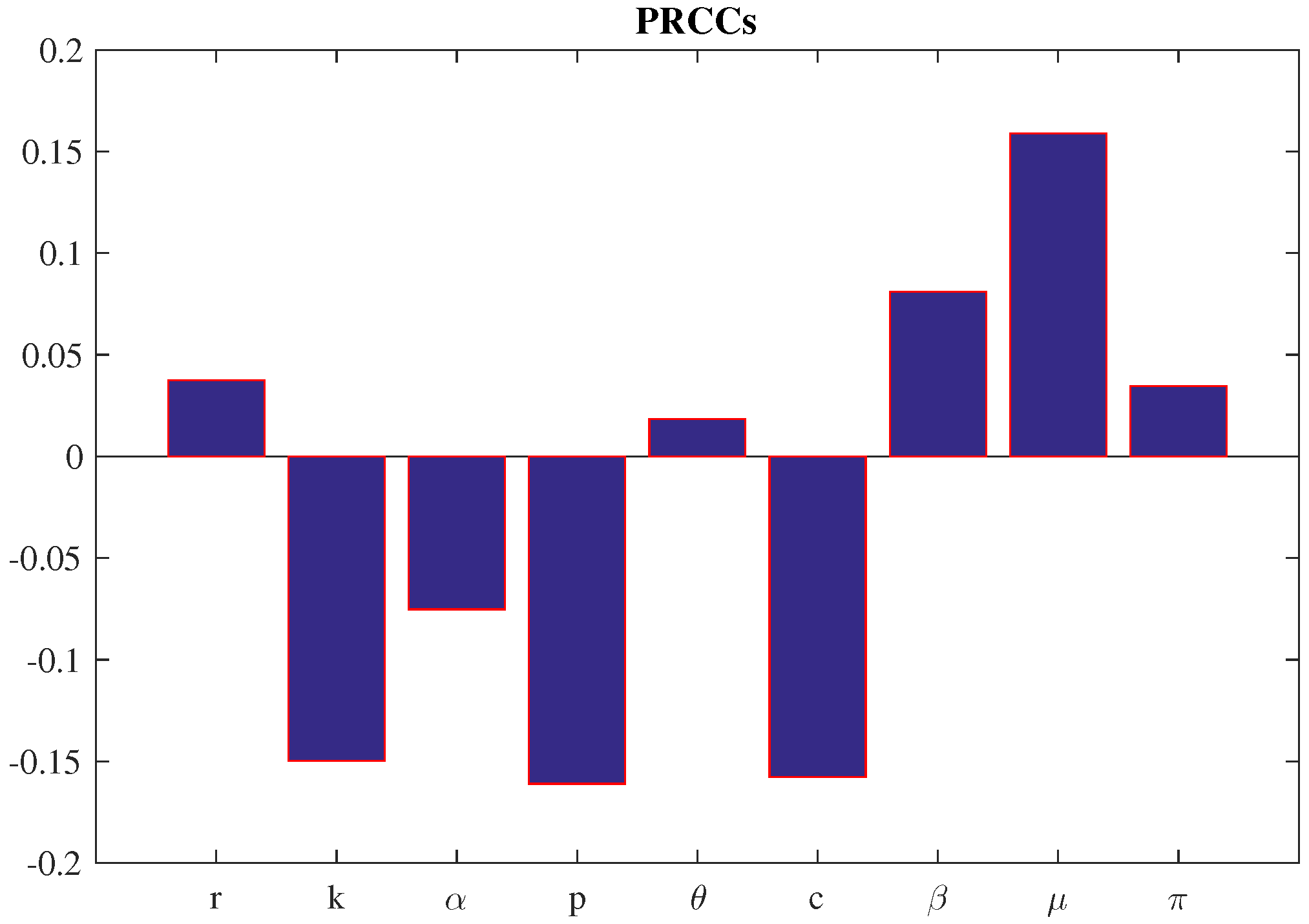
To evaluate how input parameters influence model outcomes, we conduct a sensitivity analysis. This approach helps pinpoint which variables exert the greatest impact on the dynamics of the system [30,31]. Common techniques for sensitivity analysis include Partial Rank Correlation Coefficient (PRCC), extended Fourier Amplitude Sensitivity Test (eFAST). Among these, PRCC is particularly effective for global sensitivity analysis, especially in complex, high-dimensional, and nonlinear models. It accounts for the interdependencies among variables, making it a robust choice for assessing parameter influence [29].
Before applying PRCC, we use Latin Hypercube Sampling (LHS) to generate a diverse and representative set of input values. LHS ensures efficient coverage of the parameter space, which is essential for reliable sensitivity results. Following the methodology outlined by Marino et al. [29], we performed PRCC-based sensitivity analysis on the first and second fish predator populations. This allowed us to clearly assess the relative influence of each predator on the system dynamics.
For crop biomass X, the PRCC results highlight several key parameters: and . Of these, and exhibit positive correlations with biomass, while the remaining parameters show negative associations.
6. Numerical Simulation
This sections contains the detail calculations of analytical results of previous sections using numerical values of the model parameters. The simulated are useful in finding significant results for pest management using sterile insect release technique. First, we study the results that are obtained from the system without optimal control. Then, we discussed the results of the optimal system.
Results from the system without control
Figure 1 is the analysis of the feasible roots of equation (15). We observe that two feasible interior equilibrium exits but one is stable and another is unstable i.e. bistability does not occur.
Time series solutions of the system are plotted in Figure 2 for three different values of . It is observed that as the values of are increased, oscillations in the populations are also increased. Hopf bifurcation is observed in Figure 3 when passes its critical vale (approx.). In this figure, we have plotted the maximum and minimum values of the periodic solutions with respect to the bifurcation parameter .
Another time series plot is shown in Figure 4 for different values of the rate of release of sterile male pests, . We have taken that means there is already periodic oscillation in the system. Now we increase the value of and see that the system becomes stable. Thus we conclude that role of is to stabilize the system. In Figure 5, we have plotted a Hopf bifurcation diagram for . Stability switch is observed from unstable to stable when is increased from to 2.
In Figure 6, phase portraits are plotted in different phase planes taking different initial values of the populations. It is observed that all trajectories converge to the same point (interior point, ). This shows that the for the set of parameter values, the system is globally asymptotically stable.
Regions of stability (two parameter bifurcation) of the coexisting equilibrium is shown in in parameter plane. Figure 7 shows that Region of stability decreases when the parameter values are increased. Note that (15) has two feasible roots. One is always unstable, other one is stable on the green region and unstable in yellow region. This figure also shows that the critical value of for occurrence of Hopf bifurcation depends on the value of .
A Hopf bifurcation occurs when stability of a system shifts due to a change in a parameter values, leading to the emergence of periodic behavior. This phenomenon arises when a pair of complex conjugate eigenvalues cross the imaginary axis of the phase space. Mathematically, it signifies a transition from a stable equilibrium to sustained oscillations. In ecological models, Hopf bifurcation provides insight into how population levels may transition between steady states and cyclical fluctuations as environmental or biological factors vary.

| Parameters | Definition | Values (Unit) |
|---|---|---|
| r | growth rate of plant biomass | 0.1 g day−1 |
| maximum plant biomass | 50 g m−2 | |
| maximum pests | 100 (g biomass)−1 | |
| crop consumption rate | 0.0025 g pest−1 day−1 | |
| contact rate of sterile pest with female pests | 0.0005 day−1 | |
| mortality rate of pests | 0.03 day−1 (g biomass)−1 | |
| Application rate of male sterile pests | 0.9 m−2 |
Results from the OCP
The proposed optimal control problem is solved numerically in Matlab using solver. Results of the optimal control problem are plotted in Figure 9 and Figure 9. We compare the results between the system with and without control in Figure 9. From Figure 4, we observe that recruitment rate of sterile pests (i.e. ) reduces the total pest population (male and female pests).
Figure 8.
PRCCs for the crop biomass, X, with respect to the parameters of the system. Mean values of the parameters are taken from Table 1.
Figure 8.
PRCCs for the crop biomass, X, with respect to the parameters of the system. Mean values of the parameters are taken from Table 1.
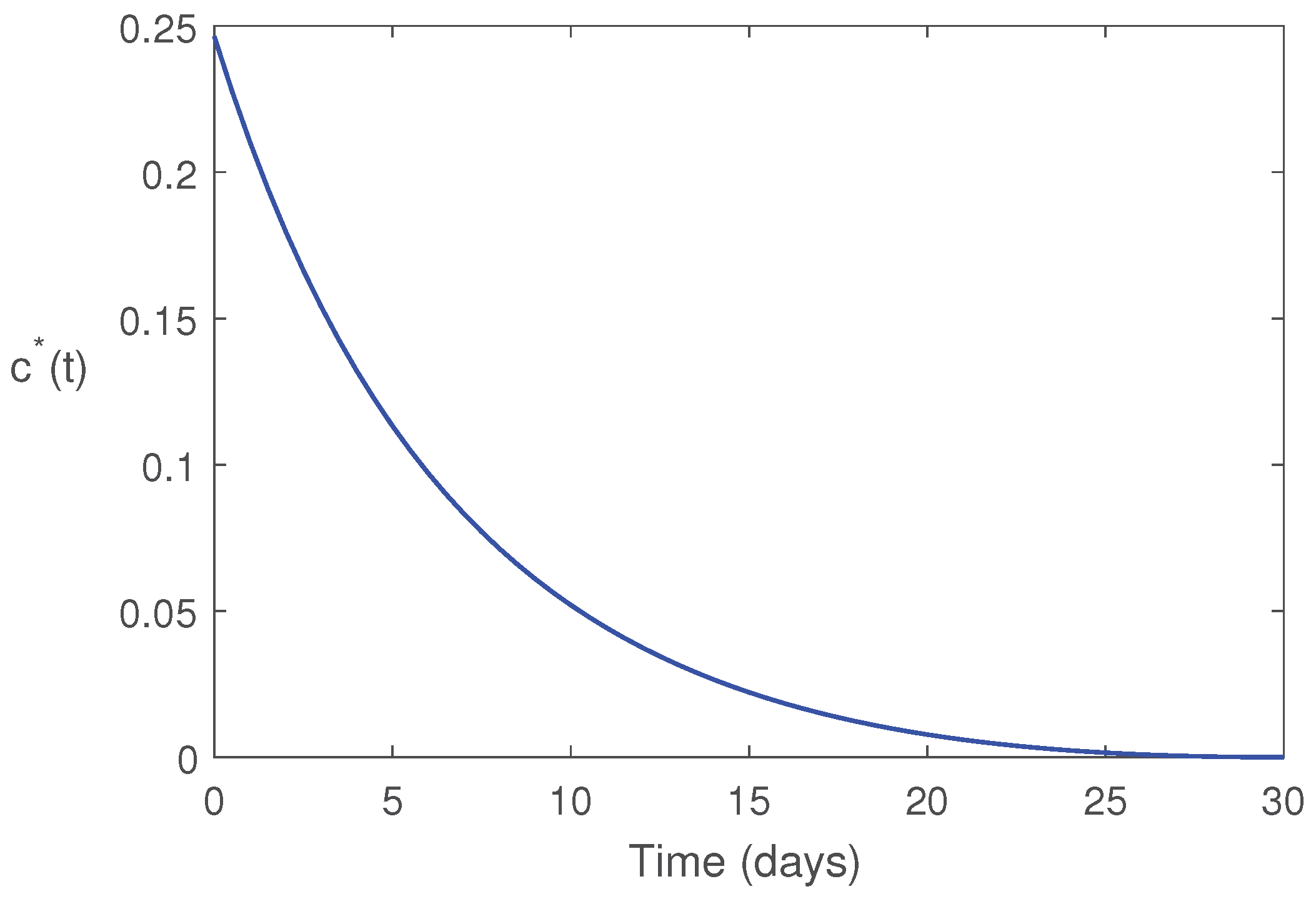
Here, we have shown that optimal use of sterile pests can minimize the pest population with minimum cost (Theorem 4). Optimal profile of the control variable is plotted in Figure 10. This shows that for minimize the cost of pest management, we should follow the trajectory of to release of sterile pests. This figure shows that initially the release rate should be high, then we have to decrease gradually the rate of release as the female pests are decreasing due to this approach.
We can say that constant release is not suitable as cost is higher. But optimal rate of release of sterile pests is significant as it minimizes the costs of pest management.
7. Discussion and Conclusion
The sterile insect technique (SIT) is a biological pest control method that involves the mass release of sterilized insects to reduce the reproductive potential of pest populations. This strategy disrupts pest population growth by preventing fertile matings, thereby suppressing infestations in agricultural systems. In this article, a mathematical model for pest control using SIT is proposed and analysed. the model contains four population: crop biomass, female pest, male pest, and sterile pests.
The proposed model has one equilibrium, the coexisting equilibrium. Stability analysis shows that the point is globally asymptotically stable when the consumption rate is lower or recruitment rate is higher. Hopf bifurcation can be observed when the rate crop consumption by pest, is higher. The critical value of depends on the other parameters of the system (Figure 7). The proposed optimal control problem shows that pest can be minimized using sterile male pests into the system when sterile pests are introduced in optimal rate.
SIT represented serves as an effective and eco-friendly method to biologically suppress pest populations. By altering the mating structure within the pest population, SIT indirectly protects the crop biomass from pests. The model helps us explore the long-term behavior of the system, including whether pest populations can be driven to low or stable levels and whether the crop biomass can recover and stabilize.
The proposed model exhibits certain limitations, notably its inability to account for stochastic phenomena such as weather variability and pest immigration, as well as spatial heterogeneity. These factors are essential for accurately representing real-world pest management scenarios.
In conclusion, the sterile insect technology is functional for crop pest management. The results obtained from the proposed mathematical model and from the optimal control problem are significant for real world application.
Data Availability Statement
Data sharing is not applicable to this article as no data sets were generated or analyzed for the current study. The dada used here are mentioned within the article.
Acknowledgments
The authors extend their appreciation to the Deanship of Research and Graduate Studies at King Khalid University for funding this work through Large Group Project under grant number (58/ 46).
Conflicts of Interest
The authors declare no conflict of interest.
References
- Sutter, A. , Price, T.A. and Wedell, N., 2021. The impact of female mating strategies on the success of insect control technologies. Current Opinion in Insect Science, 45, pp.75-83.
- van Lenteren, J.C. , 1999. Fundamental knowledge about insect reproduction: essential to develop sustainable pest management. Invertebrate reproduction & development, 36(1-3), pp.1-15.
- Ridley, M. , 1988. Mating frequency and fecundity in insects. Biological Reviews, 63(4), pp.509-549.
- Bonduriansky, R. , 2001. The evolution of male mate choice in insects: a synthesis of ideas and evidence. Biological Reviews, 76(3), pp.305-339.
- Howell, P.I. and Knols, B.G., 2009. Male mating biology. Malaria journal, 8, pp.1-10.
- Alexander, R.D. , Marshall, D.C. and Cooley, J.R., 1997. Evolutionary perspectives on insect mating. The evolution of mating systems in insects and arachnids, pp.4-31.
- Thornhill, R. , 1979. Male and female sexual selection and the evolution of mating strategies in insects. Sexual selection and reproductive competition in insects, pp.81-121.
- Bourtzis, K. and Vreysen, M.J., 2021. Sterile insect technique (SIT) and its applications. Insects, 12(7), p.638.
- Kapranas, A. , Collatz, J., Michaelakis, A. and Milonas, P., 2022. Review of the role of sterile insect technique within biologically-based pest control–an appraisal of existing regulatory frameworks. Entomologia Experimentalis Et Applicata, 170(5), pp.385-393.
- Bhandari, M.K. and Paudel, M., 2024. Genetic, biological and sterile insect techniques: Insect pest management strategies: A review. Agricultural Reviews, 45(3), pp.390-399.
- Reddy, P.V. and Rashmi, M.A., 2016. Sterile Insect Technique (SIT) as a component of area-wide integrated management of fruit flies: Status and scope. Pest Management in Horticultural Ecosystems, 22(1), pp.1-11.
- Vreysen, M.J. , Hendrichs, J. and Enkerlin, W.R., 2006. The sterile insect technique as a component of sustainable area-wide integrated pest management of selected horticultural insect pests. Journal of Fruit and Ornamental Plant Research, 14, p.107.
- Barclay, H.J. , 2021. Mathematical models for using sterile insects. In: Sterile insect technique (pp. 201-244). CRC Press.
- Bakhtiar, T. , Fitri, I.R., Hanum, F. and Kusnanto, A., 2022. Mathematical model of pest control using different release rates of sterile insects and natural enemies. Mathematics, 10(6), p.883.
- Sarkar, S. , Bhattacharyya, J. and Pal, S., 2024. Modeling and analysis of optimal implementation of sterile insect technique to suppress mosquito population. Journal of Biological Systems, 32(02), pp.859-888.
- Maru, N.K. and Sao, Y., 2018. Sterile insect technology for pest control in agriculture. Int. J. Bio-resour Stress Manag, 9(2), pp.290-305.
- Bakhtiar, T. , Fitri, I.R., Hanum, F. and Kusnanto, A., 2022. Mathematical model of pest control using different release rates of sterile insects and natural enemies. Mathematics, 10(6), p.883.
- Barclay, H.J. , 2005. Mathematical models for the use of sterile insects. In Sterile insect technique: principles and practice in area-wide integrated pest management, pp. 147-174. Dordrecht: Springer Netherlands.
- Ben Dhahbi, A. , Chargui, Y., Boulaaras, S.M., Ben Khalifa, S., Koko, W. and Alresheedi, F., 2020. Mathematical modelling of the sterile insect technique using different release strategies. Mathematical Problems in Engineering, 2020(1), p.8896566.
- Anguelov, R. , Dufourd, C. and Dumont, Y., 2017. Mathematical model for pest–insect control using mating disruption and trapping. Applied Mathematical Modelling, 52, pp.437-457.
- Bhattacharyya, S. , Bhattacharya D. K., An improved integrated pest management model under 2-control parameters (sterile male and pesticide), Mathematical Biosciences, Vol. 209, pp. 256-281, 2007.
- Al Basir, F. , Banerjee, A. and Ray, S., 2019. Role of farming awareness in crop pest management-A mathematical model. Journal of theoretical biology, 461, pp.59-67.
- Edholm, C.J. , Tenhumberg, B., Guiver, C., Jin, Y., Townley, S. and Rebarber, R., 2018. Management of invasive insect species using optimal control theory. Ecological Modelling, 381, pp.36-45.
- Vincent, T.L. , 1975. Pest management programs via optimal control theory. Biometrics, pp.1-10.
- Fitri, I.R. , Hanum, F., Kusnanto, A. and Bakhtiar, T., 2021. Optimal Pest Control Strategies with Cost-effectiveness Analysis. The Scientific World Journal, 2021(1), p.6630193.
- Fleming W., H. and Rishel R. W., Deterministic and Stochastic Optimal Control, Springer Verlag, 1975.
- Culshaw, R. V. , Rawn, S., Spiteri, R. J., Optimal HIV treatment by maximising immuno response, Journal Mathematical Biology, Vol. 48, pp. 545-562, 2004.
- Pontryagin L., S. , Boltyanskii V. G., Gamkarelidze R. V., Mishchenko, E. F., Mathematical Theory of Optimal Process. Gordon and Breach Science Publishers 4, 1986.
- Marino, S. , Hogue, I.B., Ray, C.J. and Kirschner, D.E., 2008. A methodology for performing global uncertainty and sensitivity analysis in systems biology. Journal of theoretical biology, 254(1), pp.178-196.
- Reja, S. , Ghosh, S., Ghosh, I., Paul, A. and Bhattacharya, S., 2022. Investigation and control strategy for canine distemper disease on endangered wild dog species: a model-based approach. SN Applied Sciences, 4(6), p.176.
- Sarwardi, S. , Reja, S., Al Basir, F., Raezah, A.A., 2025. Delay-induced bubbling in a harvested plankton-fish model: A study on the role of two fish predators. Nonlinear Dyn, 113, 22143–22165.
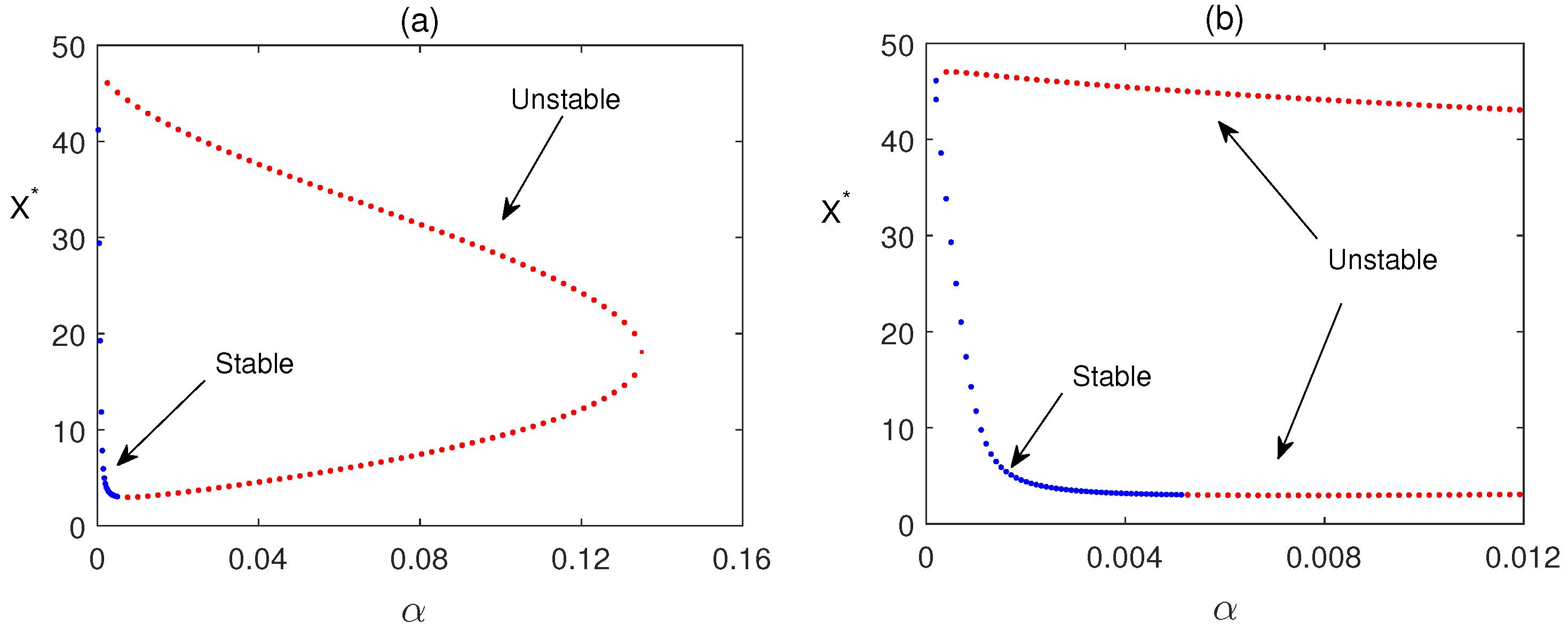
Figure 2.
Time series solutions of the system (1) for different values of (the consumption rate). Rest of the parameter values are taken from Table 1.
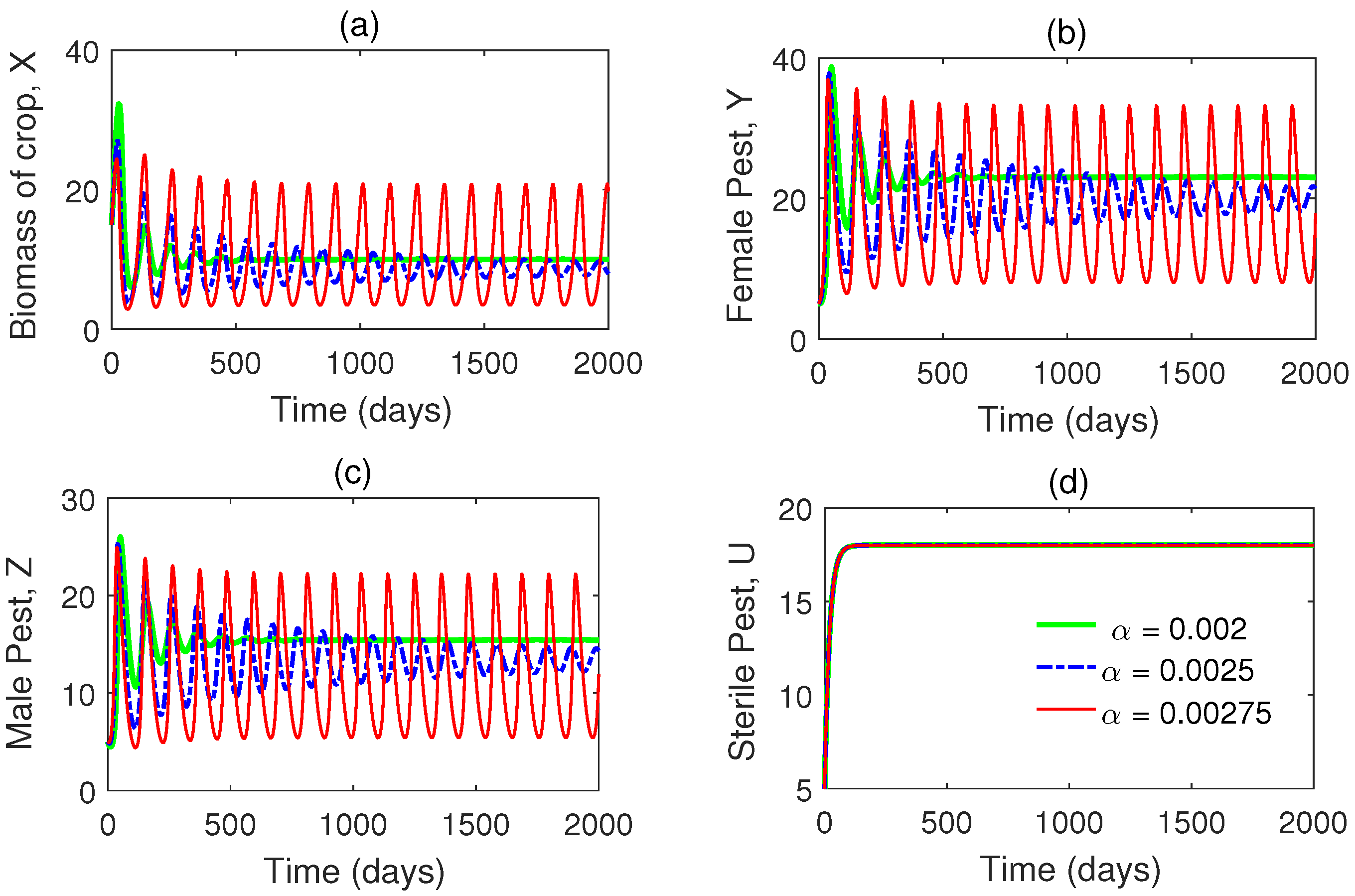
Figure 3.
Hopf bifurcation (HB) of the system (1) for . Other parameter values are taken from Figure 2.
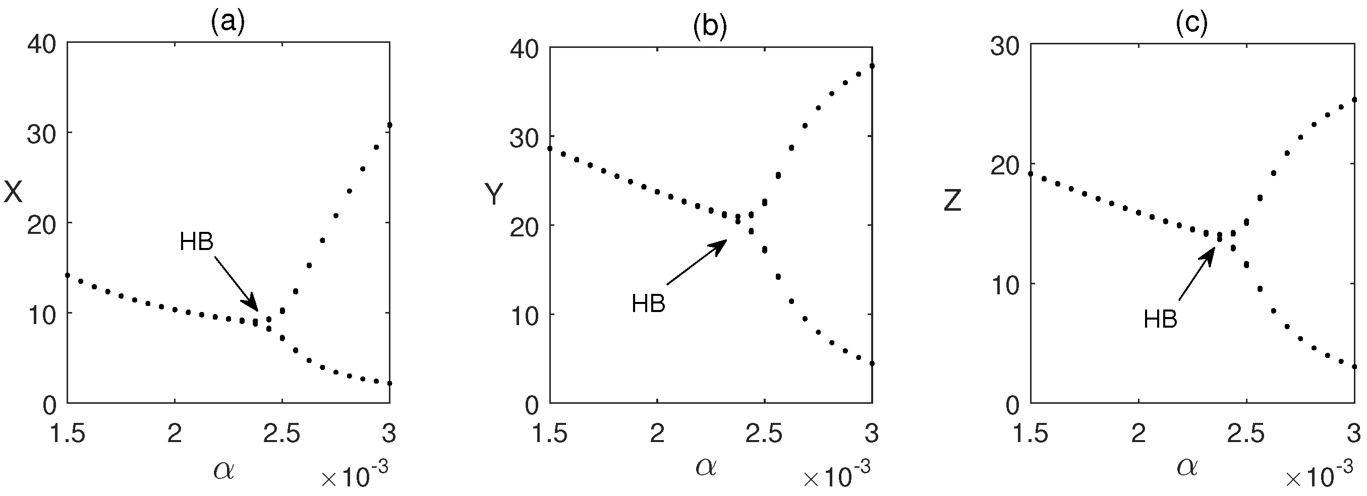
Figure 4.
Time series solutions of the system (1) for different values of (rate of recruitment of sterile pests) using the set of parameter as in Table 1 except .
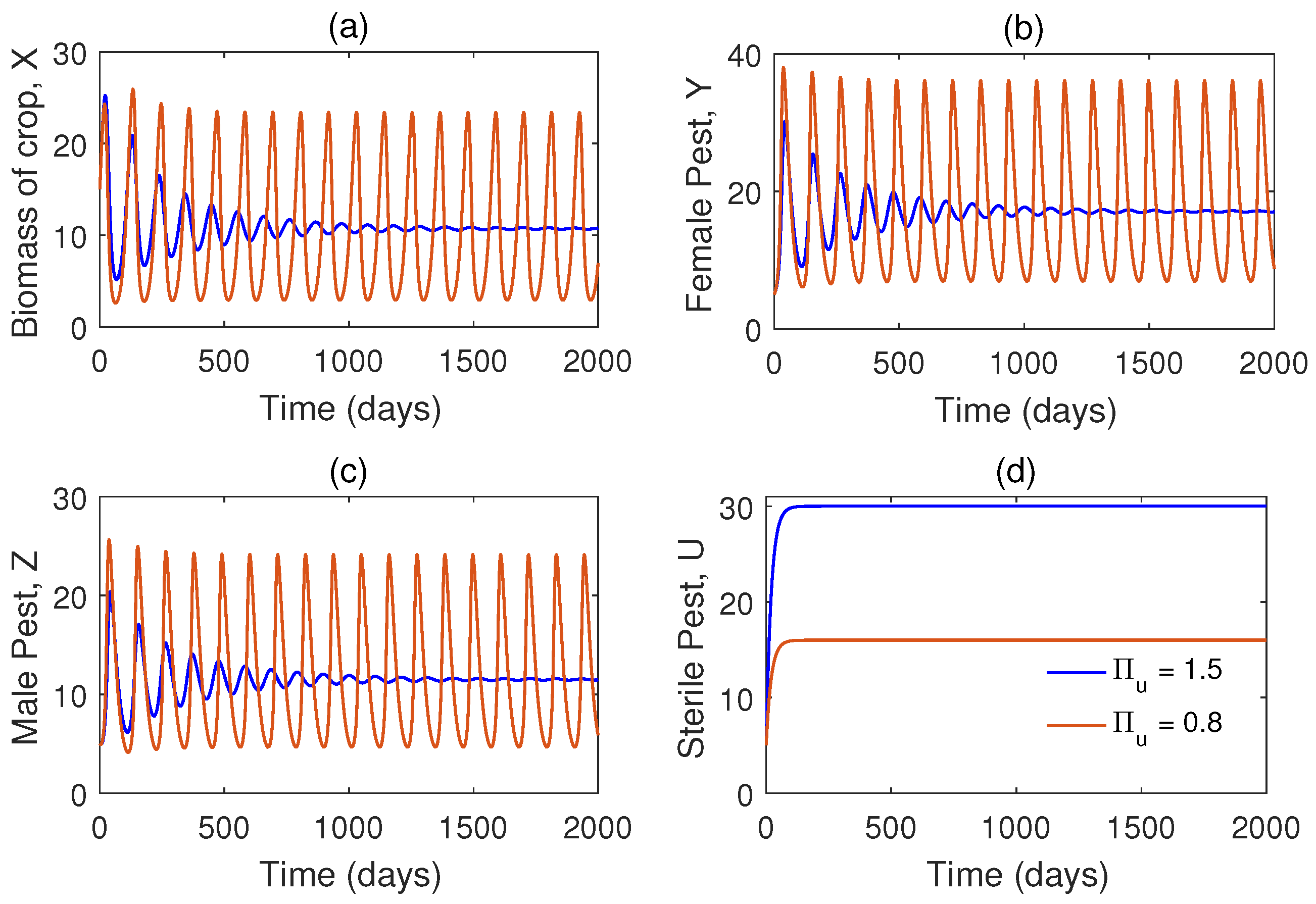
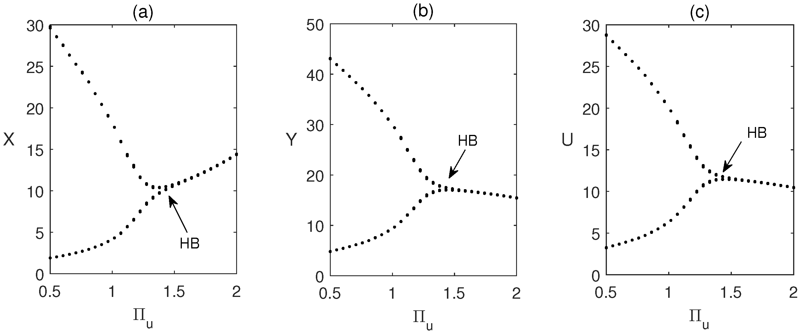
Figure 6.
Nonlinear stability of : solution trajectories are plotted for different initial values in and phase planes.
Figure 6.
Nonlinear stability of : solution trajectories are plotted for different initial values in and phase planes.
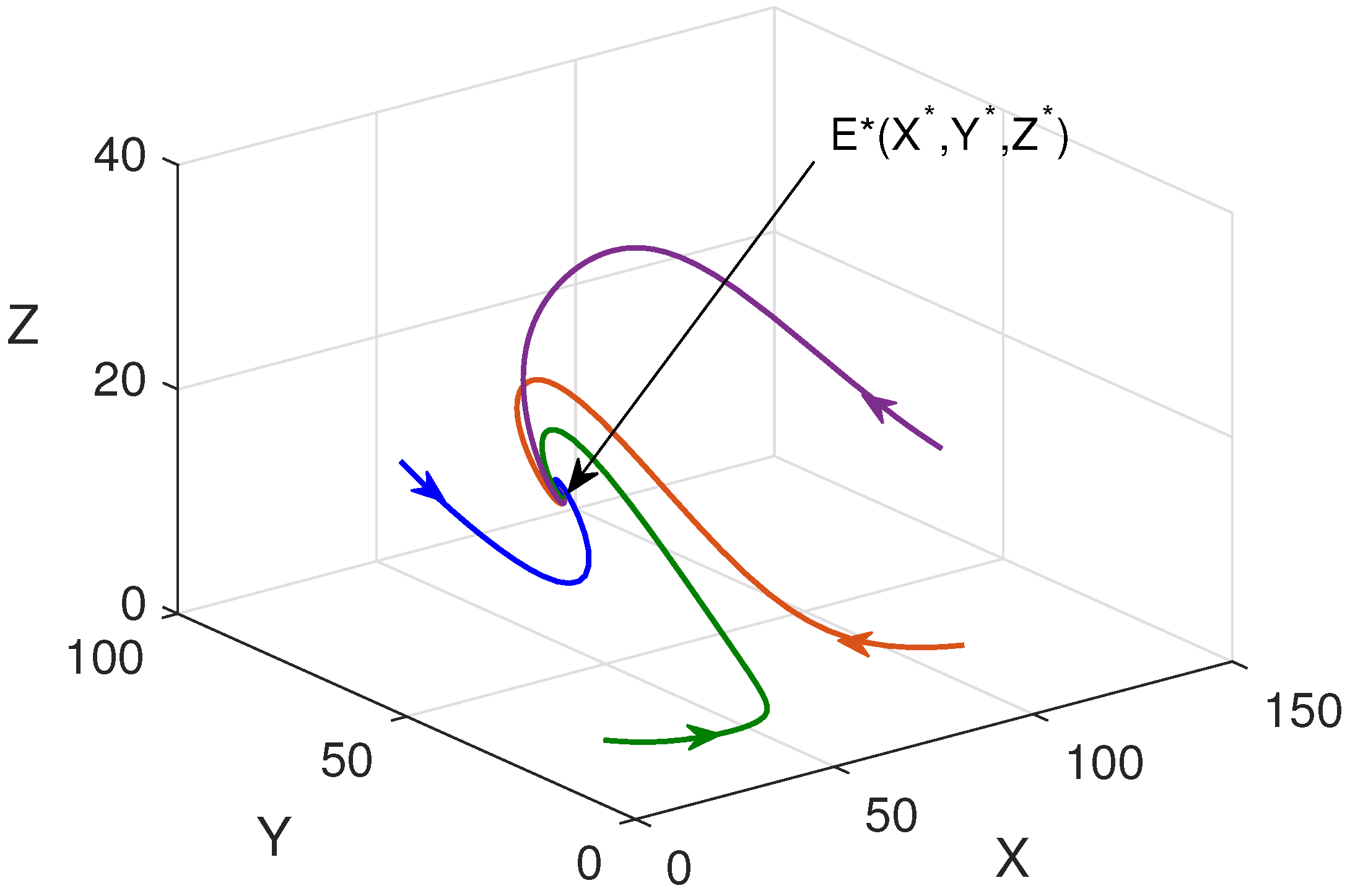
Figure 7.
Region of stability of in parameter planes. In the white region, is not feasible.
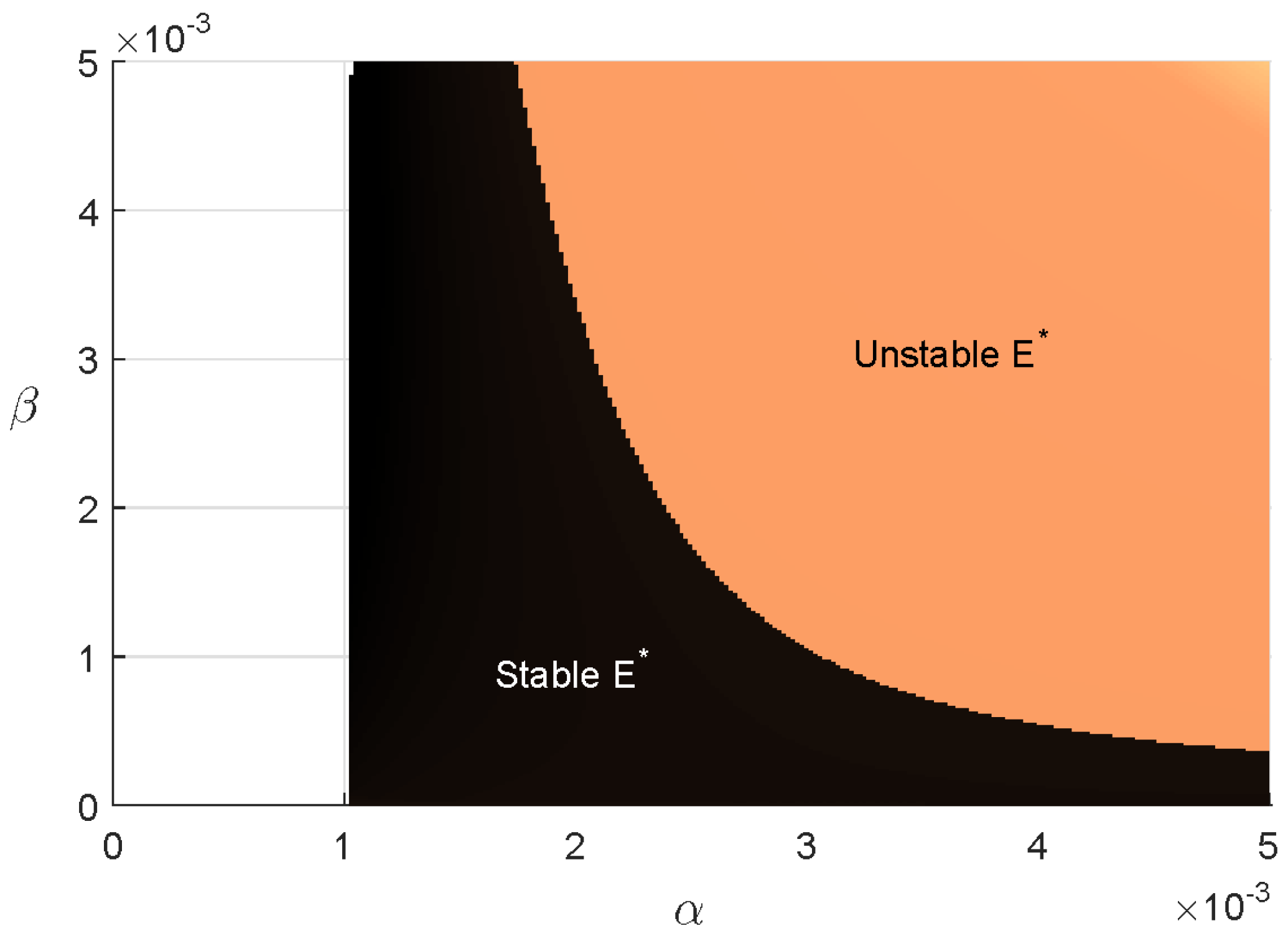
Figure 9.
Numerical solutions of the optimal control problem with parameter values as in Table 1.
Figure 9.
Numerical solutions of the optimal control problem with parameter values as in Table 1.
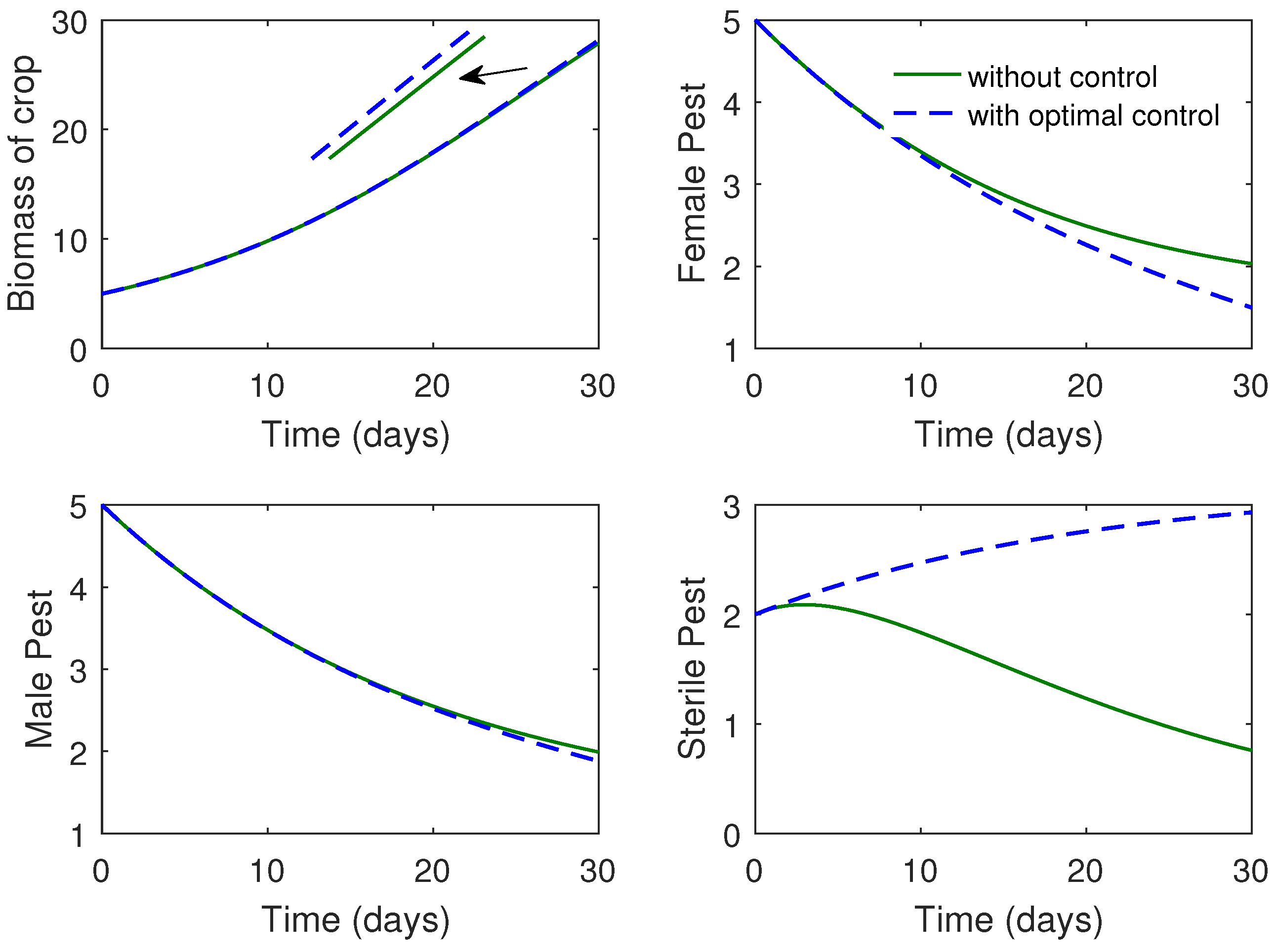
Figure 10.
Optimal control function is plotted as a function of time. Parameter values are same as in Figure 9.
Figure 10.
Optimal control function is plotted as a function of time. Parameter values are same as in Figure 9.
Disclaimer/Publisher’s Note: The statements, opinions and data contained in all publications are solely those of the individual author(s) and contributor(s) and not of MDPI and/or the editor(s). MDPI and/or the editor(s) disclaim responsibility for any injury to people or property resulting from any ideas, methods, instructions or products referred to in the content. |
© 2025 by the authors. Licensee MDPI, Basel, Switzerland. This article is an open access article distributed under the terms and conditions of the Creative Commons Attribution (CC BY) license (http://creativecommons.org/licenses/by/4.0/).
Copyright: This open access article is published under a Creative Commons CC BY 4.0 license, which permit the free download, distribution, and reuse, provided that the author and preprint are cited in any reuse.


