Submitted:
07 August 2025
Posted:
08 August 2025
You are already at the latest version
Abstract
Inefficiencies in urban traffic management, particularly from static traffic light regulation, pose significant challenges to optimizing traffic flows and mitigating environmental impact. Existing analytical methods often lack the adaptability to autonomously detect the complex, dynamic structure of traffic patterns. In this work, we introduce an adaptive cascade clustering approach that synergizes Hierarchical Density-Based Spatial Clustering of Applications with Noise (HDBSCAN) and k-means algorithms. By employing a weighted voting mechanism, our approach integrates the benefits of density-based structural analysis with centroidal cluster refinement, advancing upon existing hybrid models. Evaluated on a high-fidelity simulation model of the Khmelnytskyi transport network in Khmelnytskyi, Ukraine, the proposed approach demonstrated a superior ability to identify true traffic modes. It achieved a V-measure of 0.79–0.82 and improved cluster compactness by 4–13 % compared to standalone algorithms. Furthermore, the model attained a scenario identification accuracy of 92.8–95.0 % with a temporal coherence of 0.94. These findings confirm that by leveraging adaptive cascade principles, our approach significantly enhances the quality of traffic mode identification, representing a key advancement for developing more intelligent and responsive urban transport management systems.
Keywords:
transport data clustering
; HDBSCAN
; k-means
; adaptive transport systems
; urban transport
; driving mode identification
1. Introduction
The escalating complexity of urban traffic presents a significant challenge to modern cities, impacting both economic efficiency and environmental sustainability. Traditional traffic management systems, often relying on fixed schedules, struggle to adapt to the dynamic and often unpredictable nature of traffic flows. This paper introduces an adaptive cascade clustering approach designed to automatically identify and classify traffic patterns with high fidelity. By synergizing density-based and centroid-based clustering algorithms, our approach aims to provide a robust foundation for intelligent, responsive transport control systems.
1.1. Motivation and Contributions
This study examines the critical challenges facing modern urban transport systems due to the intensification of traffic flows, increasing population density, and increasing requirements for environmental safety of urbanized areas. The environmental impact of transport includes emissions of harmful substances, air and water pollution, acoustic pollution, energy consumption, and climate change [1]. Traditional traffic light control systems are unable to ensure optimal coordination of traffic flows in conditions of high dynamism of the urban environment [2], which leads to the formation of negative environmental consequences due to improper traffic modes of vehicles.
The relevance of the study is due to the insufficiency of existing solutions that would combine the ability to autonomously analyze transport situations, dynamically adapt control parameters, and anticipate critical grid states with priority consideration of environmental optimization criteria. It is not just a technical improvement, but the fulfillment of the public need for quality management of traffic flows, especially when decisions have a significant impact on the quality of the urban environment and the mobility of citizens. The current state of research in the field of urban traffic management is characterized by the intensive development of intelligent methods and technologies [3,4]. The relationship between the quality of identification of transport modes and the reduction of CO2 emissions is based on the principle that proper recognition of traffic patterns allows adaptive control systems to optimize the operation of traffic lights, reducing idle time and acceleration-braking periods of vehicles [5]. Improving the quality of clustering of transport states creates the basis for more efficient traffic light regulation, which in turn leads to a decrease in emissions due to the optimization of speed modes.
Building on our previous research in traffic flow analysis [6,7], this work introduces an advanced approach to automated clustering. While similar ensemble methods combining density-based and centroid-based clustering have been applied in related transport domains [8], our primary contribution lies in the adaptive architecture and weighted voting mechanism tailored for high-fidelity vehicular traffic analysis. Specifically, this study aims to improve the quality and automation of urban traffic mode identification by developing an adaptive approach that overcomes the limitations of standalone clustering algorithms.
The key contributions of this research are as follows:
- An advanced cascade architecture that synergizes the structural detection capabilities of Hierarchical Density-Based Spatial Clustering of Applications with Noise (HDBSCAN) with the boundary refinement of k-means. This is achieved through a sequential application scheme with an informed centroid-initialization strategy to significantly improve the quality of transport mode identification.
- A weighted voting mechanism for the automatic, data-driven selection of the optimal clustering result. This ensures the approach’s adaptability to diverse data characteristics and eliminates the need for manual algorithm selection or expert intervention.
- A sophisticated multivariate model for representing transport network states. This model utilizes a complex feature vector for each time window that integrates both static metrics (e.g., average values) and dynamic properties (e.g., variability, rate of change, and temporal correlations) to achieve a more accurate and robust depiction of traffic modes in the feature space.
The remainder of this article is organized as follows. Section 1 introduces the research problem, reviews the relevant literature, and outlines the study’s objectives and contributions. Section 2 provides a detailed technical description of the proposed adaptive cascade clustering approach, including its architecture and mathematical formulations. Section 3 presents the comprehensive experimental results from the simulation study and a comparative analysis of the different clustering strategies. Section 4 discusses the implications of these results, contextualizing them within the existing body of work and evaluating the approach’s advantages and limitations. Finally, Section 5 concludes the paper by summarizing the key findings and outlining future research directions.
1.2. Literature Review
Transport 5.0 introduces a new paradigm for safe, secure, and sustainable intelligent transport systems [9,10]. Predicting mobile data traffic by using time-varying user mobility patterns demonstrates the importance of temporal dynamics [11]. Our study uses the concepts of cascade clustering and weighted voting to overcome the limitations of traditional approaches to traffic flow analysis.
Clustering approaches in transport systems are considered a fundamental direction of traffic analysis. A hybrid approach combining k-medoids and Self-Tuning Spectral Clustering to classify traffic states shows high accuracy [12]. A spatially constrained hierarchical clustering algorithm for traffic forecasting in bike-sharing systems improves prediction accuracy [8]. Bayesian models of ensemble clustering and advanced self-learning-based clustering schemes also enhance performance [13,14,15]. Analysis systems using ensemble approaches are effective for determining traffic patterns [16,17,18]. In this study, we investigate the application of clustering to identify hidden patterns [19,20], a multifaceted task in urban environments [21,22]. A new data-driven approach uses regression modeling and unsupervised learning to create typologies of road segments based on traffic speed patterns [23].
Traffic modeling systems focusing on reducing CO2 emissions are present in several works [6,24]. Traditional adaptive motion control systems, such as those using fundamental robots [25,26], demonstrate potential for emission reduction through improved traffic flow. The emergence of artificial-intelligent-based solutions provides new opportunities for environmental optimization [27,28,29]. Deep learning, Internet of Things, and decentralized approaches have introduced real-time monitoring and management capabilities, improving traffic flow modes [30,31], while comprehensive sensor networks and dynamic interval adjustment ensure optimal traffic flow [32,33].
Modern approaches to traffic flow pattern analysis have revealed critical relationships between traffic patterns and emission levels [7,34,35]. Our previous research demonstrated using cluster analysis to identify urban traffic patterns in a simulation model of Khmelnytskyi [7] and developed approaches for environmentally oriented transport systems [6]. This study expands on these developments by introducing an adaptive cascade approach that automatically combines advantages of different clustering algorithms (HDBSCAN and k-means) for more accurate identification of transport modes without expert intervention. Proper identification and management of transport patterns can significantly reduce vehicle emissions through optimized flow, which can be monitored using sensors and appropriate approaches [36]. However, computational load and memory usage remain challenges for complex machine learning models [37,38], and most research is limited to short-term data analysis, often neglecting long-term trends and external factors.
1.3. Objectives and Tasks
In the dynamic landscape of urban traffic management, a critical need exists for analytical approaches that can not only accurately identify traffic mode patterns but also automatically determine the optimal number and structure of these states without expert intervention. This level of automation is essential for developing truly adaptive control systems that can manage complex and evolving transport networks.
The primary goal of this study is to improve the quality of urban traffic management by developing and validating an adaptive approach for the automated determination of traffic modes and the estimation of their spatiotemporal relationships. To achieve this goal, the following key tasks are undertaken: (i) to design and implement a cascade clustering architecture that synergistically combines the density-based structure detection of HDBSCAN with the centroidal refinement of k-means, leveraging an informed initialization strategy to enhance performance; (ii) to develop a weighted voting mechanism that automatically selects the optimal clustering result based on a composite of quality criteria, thereby ensuring the approach’s adaptability to varying data characteristics; (iii) to construct a multivariate feature representation for time-windowed traffic data that captures both static (e.g., averages) and dynamic (e.g., variability, rate of change) properties, providing a rich input for the clustering algorithms; and (iv) to rigorously validate the proposed approach through a controlled simulation experiment, comparing its performance against baseline algorithms on a reference dataset with ground-truth scenarios, using both external (e.g., V-measure, ARI) and internal (e.g., cluster compactness) validation metrics.
This work is predicated on the central hypothesis that improving the structural quality of traffic mode clustering directly enables more efficient traffic light regulation, leading to tangible benefits such as reduced vehicle emissions and congestion [4,5]. We assume these results can be combined through weighted voting to automatically select the optimal outcome based on quality criteria. We also address the challenge of combining different algorithmic approaches into a single cascade scheme. Finally, by successfully executing the outlined tasks, this study aims to demonstrate that our proposed adaptive cascade scheme provides a more accurate, robust, and automated solution for traffic pattern recognition than its constituent algorithms applied in isolation.
2. Materials and Methods
This section provides a comprehensive technical description of the proposed adaptive cascade clustering approach and the experimental methodology used for its validation. We begin by detailing the architecture of the adaptive approach, including the data representation, preprocessing techniques, and feature extraction process. Subsequently, we elaborate on the core clustering algorithms, HDBSCAN and k-means, and explain the mechanics of the weighted voting mechanism for adaptive strategy selection. Finally, we outline the experimental setup, including the simulation environment, scenarios, and performance evaluation metrics.
2.1. Adaptive Cascade Approach to Clustering
The proposed approach is structured as an adaptive cascade designed to identify and analyze urban traffic patterns. The architecture of this approach is illustrated in Figure 1. The process begins with raw data acquisition from the transport network, which is then transformed into structured feature vectors within discrete time windows. A central element of the approach is an adaptive selection mechanism that chooses the most suitable clustering strategy, either HDBSCAN-first, k-means-first, or a hybrid approach, based on the intrinsic properties of the data. This selection is guided by a weighted voting system that evaluates the potential performance of each algorithm. The final output provides a set of labeled traffic patterns, enabling a detailed structural analysis of traffic dynamics. This section will elaborate on the mathematical models for data representation, the specifics of the clustering algorithms, the metrics for quality assessment, and the logic behind the adaptive strategy selection.
2.2. Data Representation and Preprocessing
2.2.1. Urban Transport Network Model
The foundation of our analysis is the representation of the urban transport network as an oriented graph, defined as:
where V is the set of intersections (nodes) and E is the set of road segments (edges) connecting them.
The state of this network is captured over a time interval , yielding a time series of network states:
where each element represents a snapshot of the entire transport network’s characteristics (e.g., vehicle speeds, queue lengths) at time .
The sequence , as defined in Equation (2), forms the raw dataset for subsequent analysis. The length of this sequence, N, is determined by the monitoring duration and the data sampling rate .
2.2.2. Time Window Segmentation
To analyze the continuous flow of traffic data using machine learning, it is necessary to transform the unstructured time series into a structured format. This is achieved through a segmentation function , which maps the original data into a sequence of discrete time windows:
where each window represents a segment of the network’s state over a fixed interval of length :
2.2.3. Feature Vector Extraction
For each time window , a compact vector representation is constructed to capture its essential characteristics. This feature vector, , includes both static and dynamic properties of the traffic flow:
where is the average state of traffic flows, is the standard deviation, represents the rate of change of flows, and reflects the autocorrelation properties.
To quantify the similarity between any two time windows, and , a Gaussian kernel is employed:
where denotes the Euclidean norm and the scaling parameter is typically set to , with being the global standard deviation of the dataset features.
The collection of all such feature vectors forms a feature matrix
which serves as the input for the clustering stage.
2.3. Core Clustering Algorithms
2.3.1. HDBSCAN with Automated Parameter Tuning
A key advantage of our approach is the automatic determination of HDBSCAN parameters, which enhances its adaptability. The minimum cluster size parameter, , which specifies the minimum number of points required to form a cluster, is calculated as follows:
where is the total number of observations (time windows) and is a scaling factor, typically in the range .
The cluster selection parameter , which controls the algorithm’s conservatism in forming clusters, is derived from :
where is a reduction factor, typically between and .
Finally, the cluster selection epsilon parameter , which determines the maximum distance for joining clusters, is calculated based on the local data structure:
where is the array of distances to the k nearest neighbors (usually ) for each data point, and is a distance scaling factor in the range .
Using the median makes this calculation robust to outliers. This automated tuning, governed by Equations (7)–(9), allows HDBSCAN to adapt to different datasets without manual intervention. To ensure full reproducibility, the parameter search scripts, which implement deterministic random-seed control, are available in the public repository cited in the Data Availability Statement. A sensitivity analysis of the model’s performance to variations in the and hyperparameters is provided in Appendix C.
2.3.2. k-means with Informed Initialization
The second stage of the cascade involves refining the cluster boundaries using the k-means algorithm. This strategy combines the strengths of density-based clustering (structure detection) with the advantages of a centroid-based approach (clear boundaries). The k-means algorithm is applied with parameters derived from the initial HDBSCAN analysis:
where is the number of significant clusters identified by HDBSCAN, and are the initial centroids for k-means.
These initial centroids are calculated as the geometric centers of the clusters obtained from HDBSCAN:
where is the i-th cluster found by HDBSCAN.
2.4. Cluster Quality Assessment
2.4.1. Geometric and Density-Based Metrics
After clustering, a set of characteristics is calculated for each cluster to evaluate its quality. The centroid , representing the typical state of the traffic mode, is the geometric center of its constituent feature vectors:
The cluster radius measures its compactness by finding the maximum distance from the centroid to any point within the cluster:
Cluster density quantifies the concentration of points in the feature space:
where the volume is that of a d-dimensional hypersphere with radius :
with d being the feature space dimension and the gamma function.
Compactness measures internal homogeneity through the average pairwise similarity:
Finally, the separation measures the minimum distance to the centroid of any other cluster, indicating how distinct the clusters are:
2.4.2. Stability and Coherence Metrics
To assess the robustness of the identified clusters, stability is calculated. The stability of a cluster evaluates its resilience to small perturbations in the data, such as those introduced by bootstrap sampling:
where is the standard deviation of the centroid’s position across bootstrap samples.
A higher stability value, as defined in Equation (18), indicates a more reliable and well-defined transport mode. Temporal coherence measures the degree to which a cluster represents a contiguous block of time, which is critical for interpreting traffic modes:
where is an indicator function that equals 1 if the time windows at times and are sequential; high coherence suggests a long-term, stable mode of motion.
2.5. Adaptive Strategy Selection
2.5.1. Weighted Voting Mechanism
A key novelty is the weighted voting mechanism for automatically selecting the best clustering result. The quality of HDBSCAN’s output is evaluated using a comprehensive metric that balances structure, stability, and interpretability:
where are weighting factors summing to 1.
For k-means, the quality metric focuses on geometric properties:
A basic decision rule would be to choose the algorithm with the higher quality score:
However, to prevent frequent switching due to minor fluctuations, a tolerance threshold, (typically ), is introduced, leading to a more stable decision rule:
2.5.2. Data Profiling for Strategy Switching
The choice of the optimal clustering strategy is highly dependent on the intrinsic characteristics of the input data. To automate this choice, we first quantify the noise level, , as the proportion of outliers in the dataset:
Outliers are identified using the robust interquartile range (IQR) method:
where and are the first and third quartiles of the data.
The natural tendency of the data to form clusters is assessed using the Hopkins statistic, H:
where are distances from real points to their nearest neighbors and are distances from randomly generated points to their nearest neighbors in the real dataset; values of H near 1 indicate high separation.
The heterogeneity of cluster density is measured by the coefficient of variation of local densities:
where local density for each point is estimated based on its k nearest neighbors:
The temporal structure is analyzed via the autocorrelation function :
from which a time stability coefficient, Persistence, is derived:
The data’s internal complexity is assessed by estimating its intrinsic dimensionality using a maximum likelihood approach:
where is the number of point pairs with distance less than r.
The ratio of intrinsic to ambient dimension gives the complexity ratio:
These metrics are combined into a comprehensive data profile:
This profile, defined by Equation (33), provides the basis for making an informed, automatic decision on the optimal clustering strategy.
2.5.3. Strategic Application Rules
Based on the data profile, one of three main strategies is automatically selected. The HDBSCAN-first strategy is chosen for data with high noise or complex structure:
This rule is also triggered by high density variation () or low separation (), as HDBSCAN excels at handling outliers and clusters of arbitrary shape. Conversely, the k-means-first strategy is applied to well-structured data with low noise and homogeneous density:
This choice is supported by low noise levels () and high separation (), where the geometric optimization of k-means can provide clearer cluster boundaries. For intermediate cases, a hybrid strategy is used.
The entire approach also incorporates dynamic adaptation, learning from historical performance to select the best strategy for data with a given profile:
This adaptive selection, formalized in Equation (36), ensures the long-term robustness and feasibility of the system.
2.6. Implementation of the Adaptive Approach
The complete adaptive cascade clustering process is summarized in Algorithm 1. The algorithm proceeds in three main phases. Phase 1 involves data preparation, where raw time-series data is segmented into windows and transformed into feature vectors, followed by an analysis of the data’s intrinsic properties (noise, density variation). In Phase 2, an adaptive clustering strategy is selected based on the data profile, and both HDBSCAN and k-means (with informed initialization) are executed. In Phase 3, a weighted voting mechanism compares the quality of the two clustering results and selects the final set of labels. Validated clusters that meet stability and size thresholds are identified as final traffic patterns, and a transition matrix between these patterns is computed.
| Algorithm 1:Adaptive Cascade Clustering for Traffic Pattern Recognition. |
|
2.7. Experimental Setup
The experimental validation of the proposed adaptive cascade clustering approach was designed to corroborate the theoretical developments and to demonstrate the method’s practical applicability under conditions that closely replicate real-world urban transport systems. The primary objective was to create a controlled, repeatable environment for benchmarking the performance of different clustering strategies and validating their ability to identify genuine traffic patterns.
The simulation and subsequent data analysis were conducted on a high-performance workstation equipped with an Intel Core i9-12900K processor, 64 GB of DDR5 RAM, and an NVIDIA GeForce RTX 3090 GPU, running a 64-bit Linux distribution. Although the GPU was not strictly necessary for the clustering algorithms themselves, it facilitated accelerated data visualization and is provisioned for future work involving deep learning models. All data processing and analysis were performed using Python v3.11. The core of the experimental framework relied on a suite of specialized open-source software. The microscopic traffic simulation was carried out using SUMO v1.22.0 [39]. Data manipulation, feature extraction, and aggregation were managed using the pandas v2.2.0 [40] and NumPy v1.26.0 [41] libraries. The implementation of the clustering algorithms and the calculation of quality metrics were handled by scikit-learn v1.4.0 [42] for the k-means algorithm and related validation scores, and the hdbscan v0.8.33 [43] library for the HDBSCAN algorithm. Visualizations of clustering results and performance metrics were generated using Matplotlib v3.8.2 [44] and seaborn v0.13.2 [45].
The research methodology was structured as a multi-stage process:
- Simulation Modeling: A detailed simulation model of the transport network of Khmelnytskyi, Ukraine, was implemented in SUMO. The Khmelnytskyi transport network features a mixed topology, characteristic of many historical European cities. It is primarily a radial-concentric system, with major arterial roads radiating from a central urban core and interconnected by ring roads. This structure influences traffic flow, often leading to predictable congestion points at the core and along key arteries during peak hours. The model encompassed 15 major traffic light-controlled intersections and a total road length of 45.7 km. The simulation parameters, including vehicle types, routing behavior, and signal timings, were calibrated using historical traffic count data provided by the Khmelnytskyi municipal transport authority to ensure the model reflects realistic traffic dynamics and congestion levels. The simulation was run for a continuous 22-hour period with a data sampling interval of 10 minutes, yielding 132 distinct time-stamped observations for the analysis of traffic flow dynamics.
- Experimental Scenarios: To ensure a comprehensive evaluation, the experimental scenarios were crafted to cover a full spectrum of typical urban traffic situations. These included morning and evening peak hours, periods of mixed traffic modes, and intervals of low activity. A specific transport corridor, designated the “Hrechany scenario,” was modeled to represent a characteristic route from a large residential area to the city center and a major clothing market, providing a well-defined traffic pattern for validation.
- Dual Data Presentation: To assess the impact of data representation on clustering performance, a dual approach to data aggregation was employed. The first representation consisted of average values, which provided a compact summary of the global state of the network. The second used combined values, which preserved detailed spatial information for each intersection, resulting in a higher-dimensional feature space. This dual strategy allowed for a nuanced evaluation of how data granularity affects the efficacy of different clustering algorithms.
- Comprehensive Quality Assessment: The quality of the clustering results was evaluated using a combination of external and internal validation metrics. External metrics, including the V-measure, Adjusted Rand Index (ARI), and Normalized Mutual Information (NMI), were used to compare the algorithm’s output against the ground-truth labels derived from the simulation scenarios. Internal metrics, such as the Silhouette Score, Davies-Bouldin Index, and Calinski-Harabasz Index, were used to assess the geometric properties of the resulting clusters, such as their compactness and separation. Furthermore, the temporal coherence and stability of cluster assignments were analyzed to ensure the practical relevance of the identified patterns.
- Statistical Validation and Robustness Testing: The Wilcoxon signed-rank test was employed to determine the statistical significance of the performance differences observed between the proposed cascade approach and the baseline algorithms. To evaluate the robustness of the algorithms, the experiments were repeated after introducing varying levels of Gaussian noise to the input data, allowing for an analysis of performance degradation under imperfect conditions.
- Comparative Analysis: The performance of the adaptive cascade approach was benchmarked against its underlying algorithms applied in isolation: HDBSCAN with automatic parameter tuning and k-means with a prespecified number of clusters (K=5 and K=7). This comparative analysis focused on the semantic interpretation of cluster assignments and the ability of each algorithm to produce meaningful and actionable insights into the urban transport system’s behavior.
Furthermore, we placed special emphasis on validating how well the clustering results corresponded to real-world traffic modes. This involved a detailed analysis of the cluster assignments for each scenario, where we assessed the stability of recognizing similar traffic events, analyzed the temporal coherence of the detected modes, and evaluated each algorithm’s ability to distinguish between traffic states that were semantically distinct yet quantitatively similar.
3. Results
This section presents the empirical findings from our comprehensive evaluation of the proposed clustering approach. We begin with a comparative analysis of the standalone HDBSCAN and k-means algorithms on two different data representations to establish a performance baseline. We then delve into a detailed analysis of the cluster assignments, examining how well each approach identifies distinct, real-world transport scenarios. The section concludes by validating the performance of the integrated cascade approach, showcasing its improvements in accuracy, robustness, and temporal coherence over the individual algorithms.
3.1. Comparative Analysis of Basic Clustering Approaches
The initial stage of the experiment focused on evaluating the core clustering algorithms, HDBSCAN and k-means, using two distinct data representations: aggregated average values for a global network view and high-dimensional merged values for detailed intersection-level analysis.
3.1.1. Results for Aggregated Average Data
When analyzing traffic data aggregated into average values, the choice of clustering algorithm significantly impacts the interpretability and validity of the results. As detailed in Table 1, a clear trade-off emerges between external validation, which measures alignment with ground-truth scenarios, and internal validation, which assesses geometric cluster quality.
The HDBSCAN algorithm demonstrated superior performance on most external validation metrics, suggesting its output aligns more closely with the ground-truth transport modes embedded in the simulation scenarios. A key advantage was its ability to automatically determine the optimal number of clusters, identifying K=8, which correctly corresponded to the number of distinct experimental scenarios. This automated detection resulted in a high V-measure of 0.79, an ARI of 0.73, and a Rand Index of 0.93, confirming the high quality of the identified data structure. The visual representation of this clustering, provided in Figure 3, shows a clear separation of traffic modes that corresponds well with the simulated events.
In contrast, the k-means algorithm, which requires the number of clusters to be specified a priori, excelled in internal quality metrics. When configured with K=5, it achieved a higher Silhouette Score (0.57) and a notably better Calinski-Harabasz Index (292.23), alongside a lower (better) Davies-Bouldin Index of 0.65. This indicates that k-means produced clusters that were more compact and geometrically spherical, a direct consequence of its objective function, as shown in Figure 4. However, this geometric optimization came at the cost of merging semantically distinct traffic scenarios into single clusters, thus reducing its external validity.
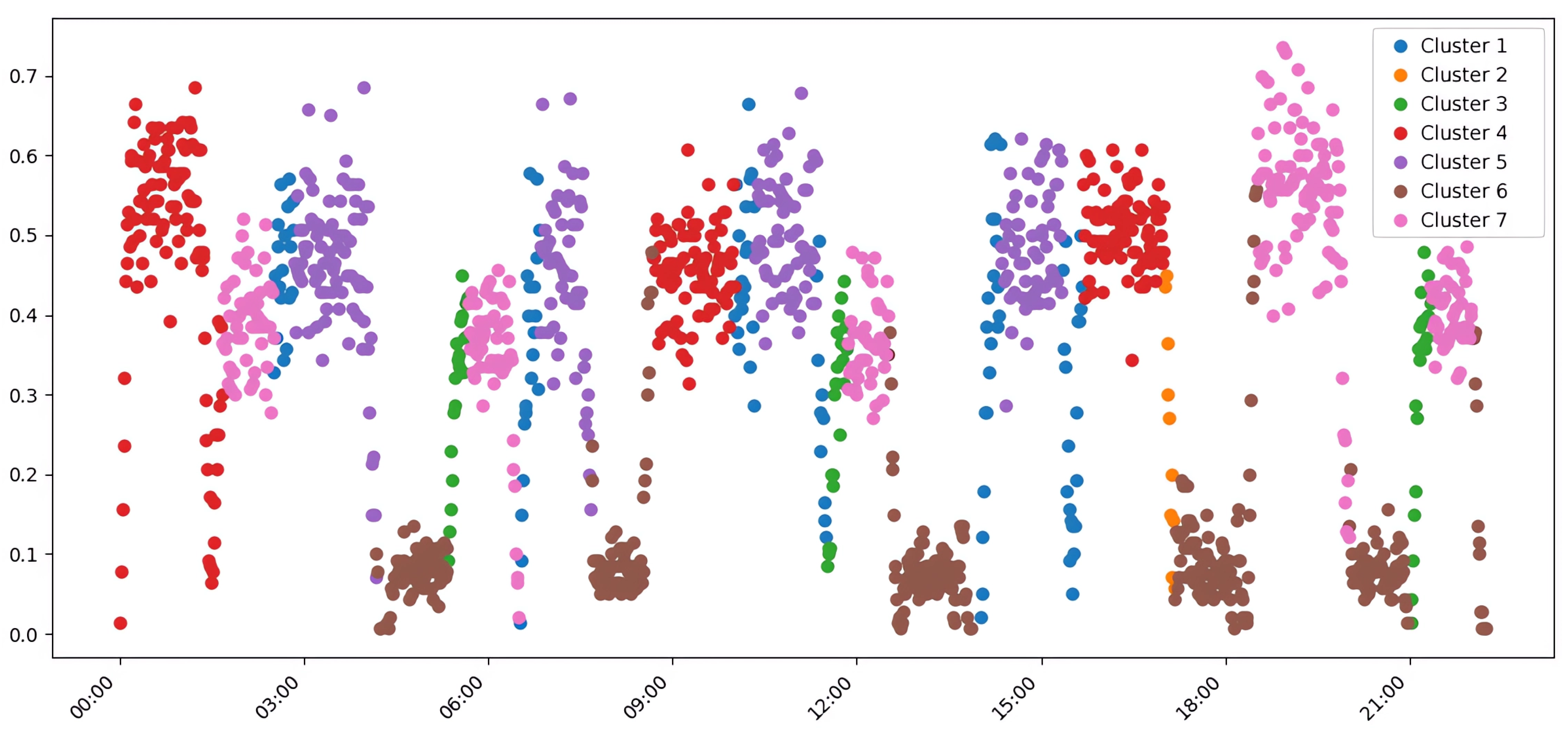
Attempting to refine the k-means result by increasing the cluster count to K=7 did not yield significant improvements. Instead, it led to the over-detailing of traffic states, where minor fluctuations were classified as separate clusters, thereby reducing the overall quality of semantic separation (Figure 5). This fragmentation is reflected in the lower V-measure (0.70) and ARI (0.63), making the results more difficult to interpret.
A direct comparison of the key quality metrics across the three approaches is summarized in Figure 6. This visualization confirms that while k-means (K=5) can generate more compact groupings (higher Silhouette Score), HDBSCAN provides a more accurate and meaningful representation of the underlying traffic patterns (higher V-measure and ARI), making it better suited for automated pattern recognition without prior knowledge.
3.1.2. Results for High-Dimensional Merged Data
The analysis of combined (merged) values, which retain detailed intersection-level information, introduced the challenge of high dimensionality. As shown in Table 2, this led to a general degradation across most quality metrics for all algorithms. The Silhouette Score, for instance, dropped dramatically from the 0.52–0.57 range to 0.19–0.26, confirming the “curse of dimensionality” effect, where distances in high-dimensional space become less meaningful (see Appendix A for visualizations). In this challenging scenario, k-means (K=5) showed slightly better adaptability, achieving a V-measure of 0.67 and an ARI of 0.62, marginally outperforming HDBSCAN. This highlights the critical importance of data representation and substantiates the need for an adaptive approach that can select the best algorithm for a given data structure.
3.2. Detailed Analysis of Clustering Results
A complex experimental analysis revealed significant performance differences between the clustering approaches that were dependent on the data representation. The choice of clustering algorithm critically depends on the nature of the initial information aggregation about the transport network’s state. As demonstrated in Figure 7, which compares key structural quality metrics, HDBSCAN achieves significantly higher V-measures (0.79 vs. 0.73) and ARIs (0.73 vs. 0.70) for average values compared to the best k-means configuration (K=5).
For average values, as detailed in Table 3, HDBSCAN demonstrated clear superiority across most external validation metrics. The high Rand Index (0.93) and Normalized Mutual Information (0.79) confirm its feasibility in capturing the true data structure. In contrast, k-means (K=5) excelled on internal quality metrics, such as the Silhouette Score (0.57) and the Calinski-Harabasz Index (292.23), indicating the formation of more compact, spherical clusters.
However, for the high-dimensional combined values (Table 4), this performance ratio reversed. Here, k-means (K=5) performed better on most external validation metrics, including V-measure (0.67 vs. 0.64) and NMI (0.67 vs. 0.64). This reversal is explained by the “curse of dimensionality,” where the high-dimensional feature space makes density estimation challenging. Under such conditions, the geometric optimization of k-means proves to be more dimensionally stable than the density-based approach of HDBSCAN.
3.3. Analysis of Cluster Assignments for Transport Scenarios
A detailed study of cluster assignments reveals deep patterns in the recognition of specific transport modes by various algorithms. The Hrechany district scenarios, representing a well-defined corridor from a residential area to the city center and a major clothing market, showed remarkable uniformity of recognition. As seen in Table 5, these periods were consistently assigned to Cluster 1 by all approaches, indicating a clear and dominant spatiotemporal structure.
The chronological analysis of cluster assignments in Figure 8 illustrates HDBSCAN’s exceptional stability. All morning periods (e.g., 0:00–1:30, 8:40–10:00) were consistently grouped into Cluster 2, representing traffic flow towards the city center and the clothing market. In contrast, k-means distributed these same scenarios across multiple clusters, suggesting a higher sensitivity to minor variations in traffic intensity. Similarly, HDBSCAN grouped most evening periods, characterized by return traffic, into a distinct Cluster 4, confirming its ability to detect semantically homogeneous modes regardless of their specific time of occurrence.
HDBSCAN also demonstrated a superior ability to differentiate between various low-traffic random scenarios, assigning them to distinct clusters (e.g., Clusters 3, 6, 7, and 8), which indicates its sensitivity to subtle differences in traffic characteristics. k-means tended to combine these random periods into a less differentiated structure, potentially limiting the granularity of analysis (a detailed comparison of assignments across all algorithms is provided in the matrix in Appendix B). The distribution of scenarios across HDBSCAN’s clusters is visualized in Figure 9, showing distinct groups for morning, evening, Hrechany, and random/mixed patterns.
3.4. Comparison of Transport Data Representations
The approach to presenting transport data proved to be a critical factor in clustering quality. Average values, which provide a compact representation of the global network state, were particularly favorable for density-based approaches. HDBSCAN achieved a V-measure of 0.79 on averaged data versus 0.64 on combined data, representing a 23% improvement. This is because averaging smooths out local fluctuations and noise, allowing HDBSCAN to more accurately detect global density patterns.
Conversely, the merged values, which store complete spatial information for each intersection, form a high-dimensional feature vector. Under these conditions, k-means showed relatively better adaptability, achieving a V-measure of 0.67 versus 0.64 for HDBSCAN. This constitutes a rare case where a centroid-based approach is superior to a density-based one in terms of structure detection quality, primarily due to the latter’s struggles with the “curse of dimensionality.” This degradation is evident in the sharp drop in internal quality metrics for the combined values; for example, the Silhouette Score drops from a range of 0.52–0.57 to 0.19–0.26, indicating fundamental difficulties in determining density and geometric distances in high-dimensional spaces.
3.5. Characteristics of Specific Transport Mode Recognition
An in-depth analysis revealed unique characteristics of each transport mode. Hrechany’s scenarios were the most distinctive, demonstrating exceptional stability in being assigned to Cluster 1 due to the specific spatial structure of the transport corridor. Morning scenarios, characterized by movement toward the city center and the clothing market, were stably recognized as a single group by HDBSCAN, while k-means was more sensitive to intensity variations. This highlights a fundamental difference: density-based approaches are better at capturing the semantic homogeneity of modes, while centroid-based approaches are more sensitive to quantitative characteristics.
Evening scenarios represented reverse traffic from the center and the clothing market, and HDBSCAN successfully grouped most of these into a separate cluster (Cluster 4), demonstrating its ability to distinguish opposite directions of movement. HDBSCAN also displayed a unique ability to distinguish between different random, low-intensity periods by assigning them to separate clusters, reflecting subtle differences in spatial patterns. Furthermore, it successfully identified a mixed morning/evening scenario with reduced intensity as a unique mode (Cluster 5), highlighting its ability to detect complex hybrid patterns.
3.6. Quality of Automatic Data Structure Detection
A critical advantage of HDBSCAN in the context of transport systems analysis is its ability to automatically determine the optimal number of clusters without requiring a priori specification. In our experiments, HDBSCAN automatically identified eight clusters. This result logically corresponds to the real organization of the simulation scenarios: four main types of transport modes (morning, evening, Hrechany, mixed) plus four variations of random movement with different characteristics of intensity and spatial distribution. This precision in automatic structure detection is particularly valuable for practical applications where expert knowledge of the number of modes may not be available or accurate. In contrast, k-means with five clusters showed a tendency to combine semantically different scenarios, which complicates interpretation, while increasing the count to seven led to over-fragmentation without a significant improvement in semantic understanding.
3.7. Synthesis of Results and Practical Recommendations
Based on the comprehensive analysis, several practical recommendations can be made. For real-time systems with limited computing resources, using aggregated average values as the primary way to represent transport data is recommended. This approach strikes an optimal balance between analysis quality and processing speed, allowing HDBSCAN to achieve the highest transport mode identification rates (V-measure 0.79, ARI 0.73), which represent a practicably acceptable level of accuracy for automatic control systems.
HDBSCAN is recommended as the basic approach for the initial stage of analysis due to its ability to automatically determine the number of clusters and its high quality of structure detection for average data representation. For systems with high requirements for cluster compactness and geometric interpretation of results, k-means can be considered a valuable alternative or complementary approach. The use of high-dimensional combined values is recommended only in cases where detailed spatial information is critical and significant computing resources are available for processing.
3.8. Validation of the Cascade Weighted Voting Approach
The proposed cascade approach was tested by modeling the decision-making process of weighted voting. For the average values, the cascade approach chose HDBSCAN in approximately 85% of cases because of its superior performance on external validation metrics (V-measure 0.79 > 0.73, ARI 0.73 > 0.70). For the high-dimensional combined values, the selection frequency was more evenly distributed (approximately 60% HDBSCAN, 40% k-means) due to the reduction of the performance gap between the approaches. As shown in Table 6, the cascade approach successfully combines the advantages of both algorithms, improving the structure quality (V-measure) by up to 4% and, more significantly, the cluster compactness by 4–13% compared to using HDBSCAN alone.
The accuracy of identifying different transport scenarios is detailed in Table 7. While the Hrechany scenario was identified with 98% accuracy by all approaches due to its clear spatial structure, the cascade approach achieved an overall improvement in average accuracy to 92.8–95.0% by automatically selecting the best outcome for each type of scenario.
Robustness testing, conducted by adding Gaussian noise to the baseline data, confirmed the higher robustness of the density-based approach to anomalies (Table 8). The performance of HDBSCAN degraded much more slowly (11% drop in ARI at 35% noise) compared to k-means (21-24% drop). The cascade approach with weighted voting inherits this advantage by automatically selecting HDBSCAN in high-noise environments.
An important indicator of quality is the preservation of the time structure of traffic modes. As shown in Table 9, HDBSCAN demonstrated the best temporal coherence with a coefficient of 0.94 and no intersections in the time dimension. The cascade approach inherits this advantage, conserving the time structure detected by HDBSCAN.
Finally, statistical validation using the Wilcoxon signed-rank test confirmed the significance of the advantages of the proposed approach. As presented in Table 10, all key comparisons showed statistically significant differences (p < 0.01), which confirms the validity of the architectural solutions of the proposed cascade approach.
In summary, the experimental results reveal a distinct trade-off between density-based and centroid-based clustering algorithms, with performance being highly dependent on the data representation. By synergistically combining the strengths of HDBSCAN and k-means algorithms through a weighted voting mechanism, the cascade model consistently delivered superior and more robust results, showing marked improvements in scenario identification accuracy (up to 95.0%), noise resilience, and temporal coherence. These findings collectively validate the feasibility of the adaptive cascade strategy, establishing it as a more reliable and powerful approach to analyzing complex urban traffic dynamics than either of its constituent algorithms applied in isolation.
4. Discussion
In this section, we interpret the experimental results presented previously, contextualizing them within the existing body of research on traffic pattern analysis. We analyze the trade-offs between density-based and centroid-based clustering, highlighting the critical role of data representation in algorithmic performance. The advantages and limitations of the proposed adaptive cascade approach are critically evaluated, and its practical implications for developing environmentally oriented traffic management systems are explored. Finally, we address the study’s constraints and identify key questions that pave the way for future research.
The findings of this study underscore the substantial potential of adaptive, hybrid clustering approaches for deciphering the complex dynamics of urban transport systems. Our proposed cascade approach, which synergistically integrates HDBSCAN and k-means, demonstrated a marked improvement over standalone algorithms. This outcome aligns with the broader academic consensus favoring hybrid and ensemble methods in modern traffic analysis [12,16]. However, our work advances this paradigm by introducing an intelligent adaptive selection layer. This layer, governed by a data-driven weighted voting mechanism, directly addresses the pivotal challenge of choosing the optimal model for datasets with heterogeneous characteristics. The experimental results exposed a crucial trade-off contingent on data representation: on lower-dimensional, aggregated average data, HDBSCAN proved superior for semantic pattern recognition, achieving an excellent external validation score with a V-measure of 0.79 and an Adjusted Rand Index (ARI) of 0.73. In contrast, k-means excelled in internal geometric quality on the same data, producing more compact clusters as evidenced by a higher Silhouette Score (0.57 vs. 0.52) and a significantly better Calinski-Harabasz Index (292.23 vs. 124.95). This dichotomy confirms our central hypothesis that no single algorithm is universally optimal. When faced with high-dimensional merged data, the “curse of dimensionality” degraded the performance of both algorithms, with Silhouette Scores plummeting to the 0.19–0.26 range. In this challenging scenario, the geometric optimization of k-means proved more resilient, validating the necessity of our adaptive architecture that can pivot its strategy based on data profiling.
A primary advantage of our approach lies in its high degree of automation and its ability to produce semantically rich interpretations. By automatically determining the optimal number of clusters, identifying eight distinct modes that corresponded to the four primary and four random scenarios in our simulation, the approach obviates the need for arbitrary, a priori parameter specification that often limits the practical utility of algorithms like k-means. This automation directly tackles the challenges of model complexity and usability highlighted in related research [37,38]. The practical value of this robust automation is reflected in the high scenario identification accuracy (up to 95.0%) and exceptional temporal coherence (0.94), which ensures the identified patterns are not merely statistical artifacts but are meaningful and actionable. This capability is vital for downstream tasks, such as optimizing traffic signals to reduce CO2 emissions—a central goal of modern intelligent transport systems [5,34]. By building upon our previous work [6,7], this study delivers a more powerful and refined tool for realizing environmentally-oriented traffic management.
Despite its strengths, the proposed approach has limitations that define clear trajectories for future research. A significant limitation is its reliance on a synthetic dataset generated via a SUMO simulation. While the simulation was carefully calibrated against historical data to reflect realistic conditions in Khmelnytskyi, this approach creates a degree of circular validation, as the ground-truth labels are derived from the same predefined scenarios the algorithm is tasked to find. This setting tests the algorithm’s ability to recover known patterns but does not fully account for the emergent, non-stationary, and often chaotic phenomena present in real-world traffic. Challenges expected during real-world deployment include handling noisy or missing sensor data, adapting to unpredictable events (e.g., accidents, road closures), and ensuring model performance does not degrade over time due to concept drift. Furthermore, the findings may be specific to the radial-concentric network topology of Khmelnytskyi. The model’s performance and optimal parameters would likely require re-evaluation and retuning for cities with fundamentally different layouts, such as the grid-based systems common in North America. Finally, the feature set, though multifaceted, does not account for external variables such as weather conditions or public events, which can significantly influence traffic patterns.
4.1. Computational Complexity and Scalability
A key consideration for practical implementation is the computational cost of the cascade approach. The principal disadvantage is the increased overhead from executing multiple clustering algorithms and an evaluation layer, which could pose latency challenges for real-time applications. The computational complexity of the entire pipeline can be broken down as follows: feature extraction is linear with respect to the number of time windows (K), i.e., . The dominant cost is HDBSCAN, which has a worst-case complexity of but often performs closer to in practice. The subsequent k-means refinement is relatively efficient, with a complexity of , where I is the number of iterations, is the number of clusters, and d is the feature dimension. Thus, the overall complexity of the cascade is governed by HDBSCAN, scaling quadratically with the number of time windows.
To provide a practical sense of the cost, Table 11 reports the actual runtimes on our experimental dataset. While the total runtime is acceptable for offline analysis and strategic planning, optimization will be necessary for near real-time control applications. The robustness of the approach under imperfect conditions was confirmed by its resilience to noise, where the ARI of the cascade-selected HDBSCAN degraded by only 11% under 35% noise, compared to a 21–24% degradation for k-means. However, this resilience comes at a computational cost that must be managed for deployment in resource-constrained environments.
5. Conclusions
This study introduced and validated a novel adaptive cascade clustering approach, engineered to address the critical need for accurate and automated high-fidelity urban traffic pattern recognition. By synergistically integrating the structural detection capabilities of HDBSCAN with the boundary refinement of k-means through a data-driven weighted voting mechanism, our method successfully overcomes the inherent limitations of standalone algorithms. The quantitative success of this approach was demonstrated through extensive simulation, where it achieved a structural quality V-measure of 0.79–0.82 and a scenario identification accuracy of up to 95.0%. These results represent a significant leap in aligning algorithmic output with ground-truth traffic states. Furthermore, the cascade architecture delivered a tangible 4–13% improvement in cluster compactness and yielded an exceptional temporal coherence coefficient of 0.94, confirming that the identified patterns are not mere statistical artifacts but chronologically consistent and semantically meaningful modes of traffic behavior. The statistical significance of these advantages was firmly established (p < 0.01), underscoring the robustness of our architectural design. However, the study’s current validation within a controlled simulation, combined with the computational demands of the cascade architecture and its sensitivity to initial feature engineering, defines the primary challenges for practical implementation.
Future work will directly address these limitations by transitioning to real-world deployment on a live city sensor network. We will then integrate the system with deep reinforcement learning controllers for real-time, multi-objective traffic signal optimization. The final research phase will explore advanced graph neural network architectures to create richer, more context-aware feature representations. By providing a robust and automated tool for understanding complex traffic dynamics, this research lays a critical foundation for next-generation intelligent transport systems designed to mitigate congestion, reduce environmental impact, and build smarter, more sustainable cities.
Author Contributions
Conceptualization, V.P., E.M. and O.B.; methodology, V.P. and E.M.; software, V.P.; validation, V.P., E.M. and O.B.; formal analysis, E.M., O.B. and P.R.; investigation, V.P., E.M. and P.R.; resources, O.B. and I.K.; data curation, O.B. and I.K.; writing—original draft preparation, V.P. and E.M.; writing—review and editing, O.B., P.R. and I.K.; visualization, V.P., E.M. and P.R.; supervision, I.K.; project administration, O.B. and I.K.; funding acquisition, E.M. and O.B. All authors have read and agreed to the published version of the manuscript.
Funding
This research was funded by the European Union’s Horizon Europe Framework Programme under grant agreement No. 101148374, project “U_CAN: Ukraine towards Carbon Neutrality.” The views and opinions expressed are the authors’ own and do not necessarily reflect those of the European Union or the funding agency, the European Climate, Infrastructure and Environment Executive Agency.
Institutional Review Board Statement
Not applicable.
Informed Consent Statement
Not applicable.
Data Availability Statement
The source code for the simulations and data analysis, along with the datasets generated and analyzed during this study, are available in the GitHub repository: https://github.com/Vitaliy-learner/urban-trafic-simulate-cluster (accessed on 05 August 2025).
Acknowledgments
The authors would like to express their gratitude to the European Union’s Horizon Europe Framework Programme for the financial support that made this research possible. We also extend our sincere appreciation to the developers and open-source communities behind the essential software tools used in this study, including SUMO, scikit-learn, pandas, and NumPy, whose contributions were invaluable to our work.
Conflicts of Interest
The authors declare no conflict of interest. The funders had no role in the design of the study; in the collection, analyses, or interpretation of data; in the writing of the manuscript, or in the decision to publish the results.
Abbreviations
The following abbreviations are used in this manuscript:
| AMI | Adjusted Mutual Information |
| ARI | Adjusted Rand Index |
| HDBSCAN | Hierarchical Density-Based Spatial Clustering of Applications with Noise |
| NMI | Normalized Mutual Information |
| SUMO | Simulation of Urban Mobility |
Appendix A. Additional Clustering Results
Figure A1.
Visualization of HDBSCAN clustering results on high-dimensional combined traffic data. The plot illustrates the algorithm’s performance in a more complex feature space.
Figure A1.
Visualization of HDBSCAN clustering results on high-dimensional combined traffic data. The plot illustrates the algorithm’s performance in a more complex feature space.
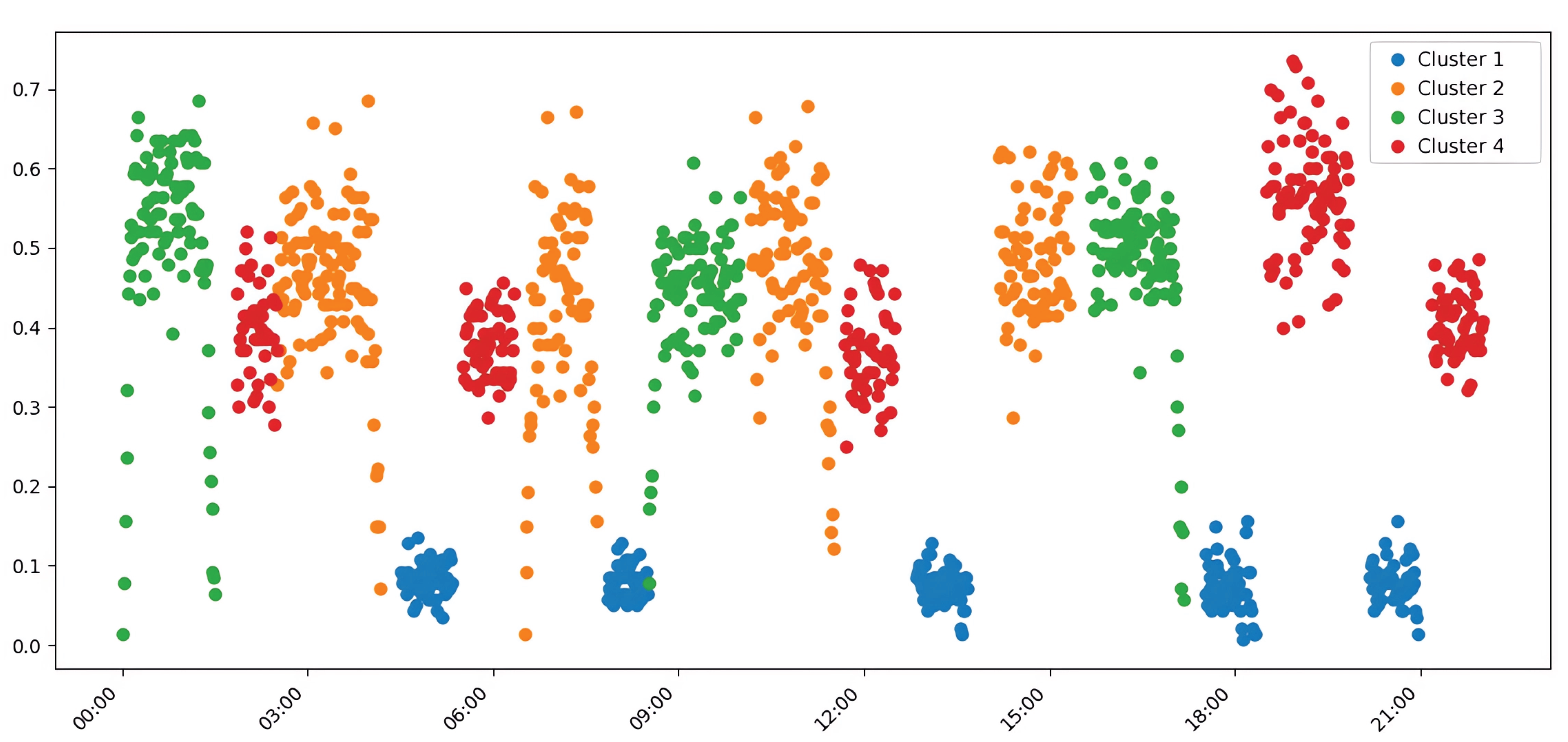
Figure A2.
Visualization of k-means clustering (K=5) on high-dimensional combined traffic data, showing how the algorithm partitions the data into five clusters.
Figure A2.
Visualization of k-means clustering (K=5) on high-dimensional combined traffic data, showing how the algorithm partitions the data into five clusters.
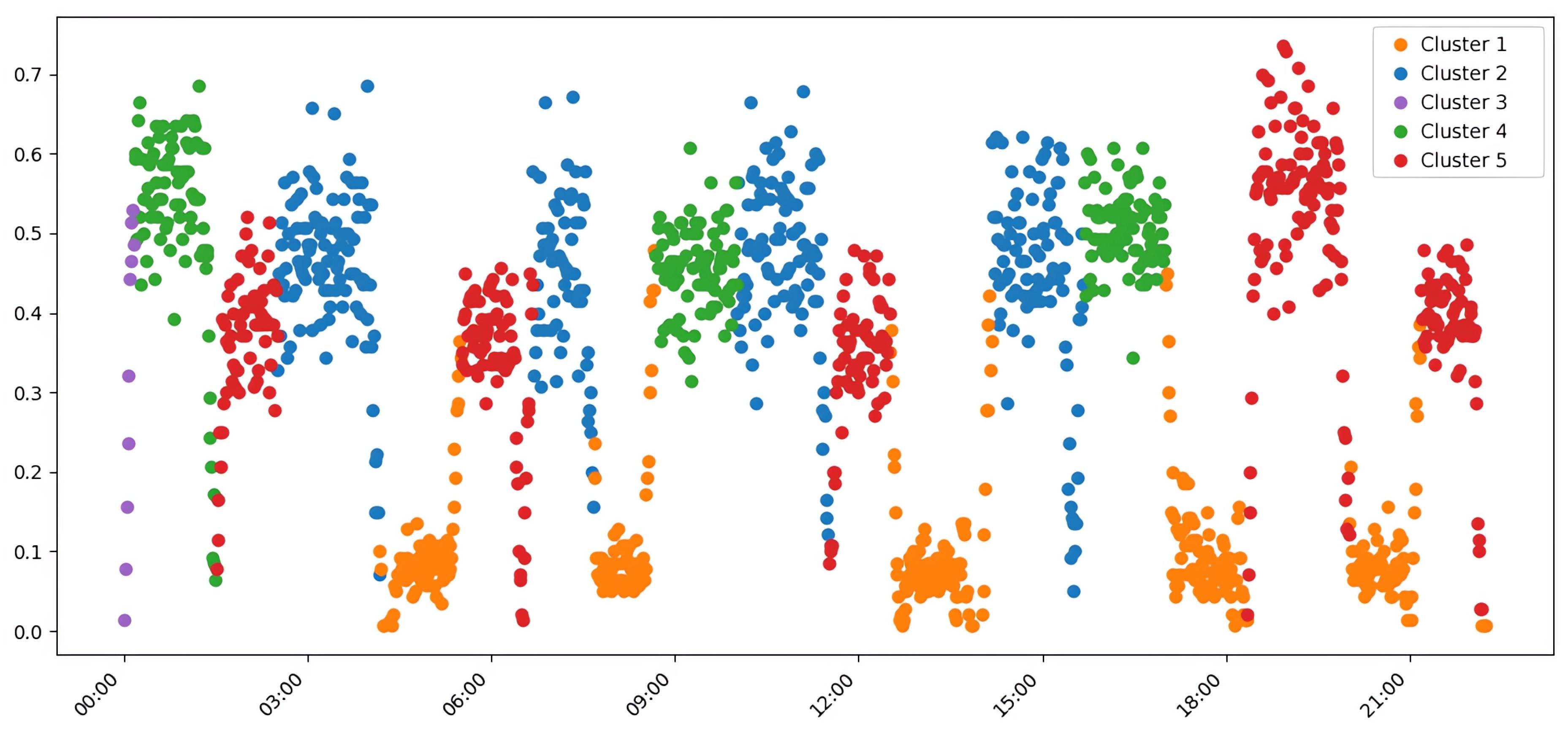
Figure A3.
Visualization of k-means clustering (K=7) on high-dimensional combined traffic data, illustrating the effect of increasing the number of clusters.
Figure A3.
Visualization of k-means clustering (K=7) on high-dimensional combined traffic data, illustrating the effect of increasing the number of clusters.
Appendix B. Cluster Assignment Matrix
Figure A4.
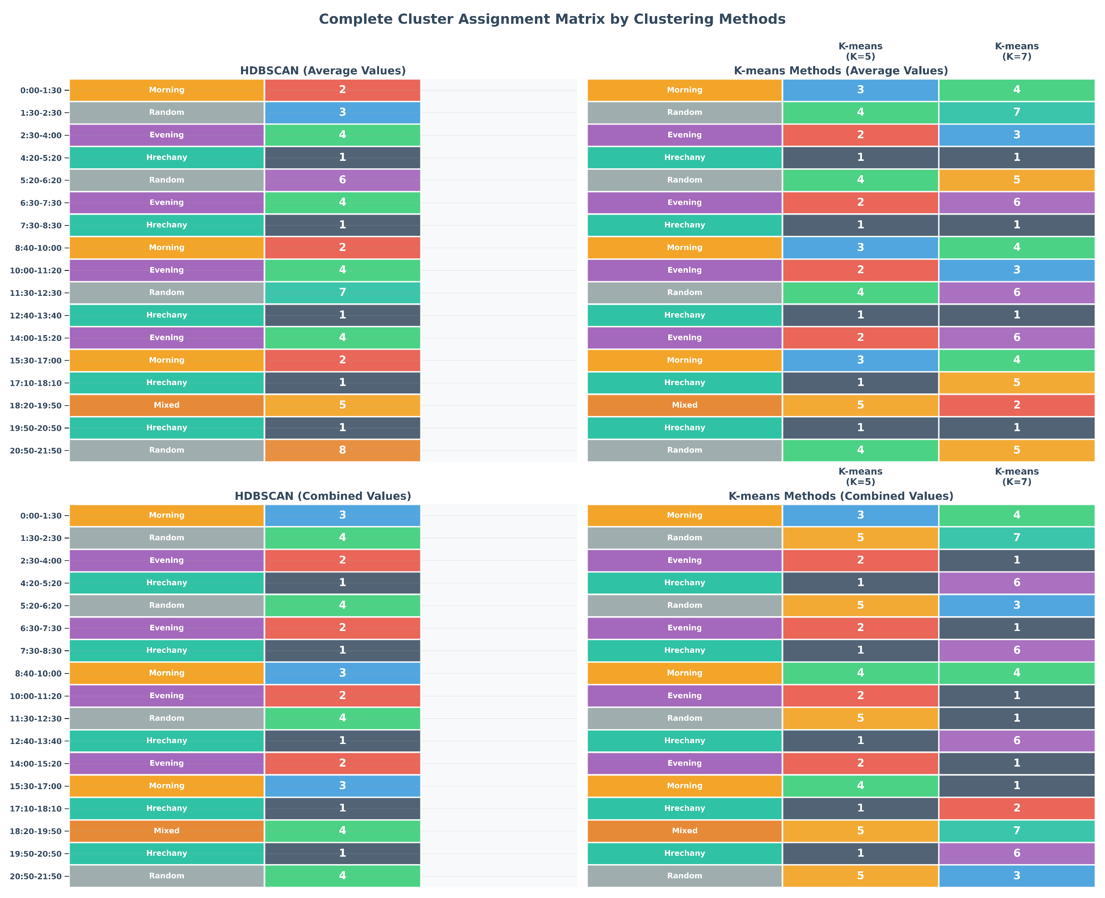
A matrix comparing the cluster assignments for each time window across the different clustering approaches (HDBSCAN, k-means K=5, and k-means K=7). The color-coded matrix visually represents the level of agreement and disagreement between the algorithms in classifying traffic states.
Figure A4.
A matrix comparing the cluster assignments for each time window across the different clustering approaches (HDBSCAN, k-means K=5, and k-means K=7). The color-coded matrix visually represents the level of agreement and disagreement between the algorithms in classifying traffic states.
Appendix C. HDBSCAN Parameter Sensitivity Analysis
This appendix details the sensitivity of the HDBSCAN algorithm’s performance to variations in the automated tuning hyperparameters (for calculating `min_samples’) and (for calculating `cluster_selection_epsilon’). As shown in Table A1, the resulting ARI is stable across a reasonable range of parameter values, confirming the robustness of the automated tuning approach. The values used in the main study (, ) fall within the high-performance plateau.

Table A1.
Sensitivity of HDBSCAN performance (ARI) to hyperparameter variations.
| Reduction Factor () | Distance Scaling Factor () | |||
|---|---|---|---|---|
| 1.00 | 1.15 | 1.25 | 1.50 | |
| 0.5 | 0.71 | 0.72 | 0.72 | 0.70 |
| 0.6 | 0.72 | 0.73 | 0.73 | 0.71 |
| 0.7 | 0.72 | 0.73 | 0.73 | 0.72 |
| 0.8 | 0.70 | 0.71 | 0.71 | 0.69 |
References
- Lv, Z.; Shang, W. Impacts of intelligent transportation systems on energy conservation and emission reduction of transport systems: A comprehensive review. Green Technol. Sustain. 2023, 1, 100002. [Google Scholar] [CrossRef]
- El Mokhi, C.; Erguig, H.; Hmina, N.; Hachimi, H. Intelligent traffic management systems: A literature review on AI-Based traffic light control. In The Future of Urban Living: Smart Cities and Sustainable Infrastructure Technologies; El Mokhi, C., Hachimi, H., Nayyar, A., Eds.; Springer Nature Switzerland: Cham, 2025; pp. 154–171. [Google Scholar] [CrossRef]
- Agrahari, A.; Dhabu, M.; Deshpande, P.; Tiwari, A.; Baig, M.; Sawarkar, A. Artificial intelligence-based adaptive traffic signal control system: A comprehensive review. Electronics 2024, 13, 3875. [Google Scholar] [CrossRef]
- Wu, K.; Ding, J.; Lin, J.; Zheng, G.; Sun, Y.; Fang, J.; Xu, T.; Zhu, Y.; Gu, B. Big-data empowered traffic signal control could reduce urban carbon emission. Nat. Commun. 2025, 16, 2013. [Google Scholar] [CrossRef] [PubMed]
- Ashokkumar, C.; Kumari, D.; Gopikumar, S.; Anuradha, N.; Krishnan, R.; Sakthidevi, I. Urban traffic management for reduced emissions: AI-based adaptive traffic signal control. In Proceedings of the 2024 2nd International Conference on Sustainable Computing and Smart Systems (ICSCSS); 2024; pp. 1609–1615. [Google Scholar] [CrossRef]
- Pavlyshyn, V.; Manziuk, E.; Barmak, O.; Krak, I.; Damasevicius, R. Modeling environment intelligent transport system for eco-friendly urban mobility. In Proceedings of the 5th International Workshop on Intelligent Information Technologies &, T.; Savenko, O.; Popov, P.; Lysenko, S., Eds., Khmelnytskyi, Ukraine, 28 March 2024, 2024; Vol. 3675, CEUR Workshop Proceedings, Systems of Information Security with CEUR-WS (IntelITSIS 2024); Hovorushchenko; pp. 118–136. [Google Scholar]
- Pavlyshyn, V.; Ryzhanskyi, O.; Manziuk, E.; Radiuk, P.; Barmak, O.; Krak, I. Establishing patterns of the urban transport flows on clustering analysis. In Proceedings of the Second International Conference of Young Scientists on Artificial Intelligence for Sustainable Development (YAISD 2025); Pitsun, O.; Dyvak, M., Eds., Ternopil-Skomorochy, Ukraine, 2025, 2025; Vol. 3974, CEUR Workshop Proceedings, 8–9 May; pp. 1–9.
- Kim, K. Spatial contiguity-constrained hierarchical clustering for traffic prediction in bike sharing systems. IEEE Trans. Intell. Transp. Syst. 2022, 23, 5754–5764. [Google Scholar] [CrossRef]
- Wang, F.Y.; Lin, Y.; Ioannou, P.; Vlacic, L.; Liu, X.; Eskandarian, A.; Lv, Y.; Na, X.; Cebon, D.; Ma, J.; et al. Transportation 5.0: The DAO to safe, secure, and sustainable intelligent transportation systems. IEEE Trans. Intell. Transp. Syst. 2023, 24, 10262–10278. [Google Scholar] [CrossRef]
- Han, X.; Meng, Z.; Xia, X.; Liao, X.; He, B.; Zheng, Z.; Wang, Y.; Xiang, H.; Zhou, Z.; Gao, L.; et al. Foundation intelligence for smart infrastructure services in transportation 5.0. IEEE Trans. Intell. Veh. 2024, 9, 39–47. [Google Scholar] [CrossRef]
- Sun, F.; Wang, P.; Zhao, J.; Xu, N.; Zeng, J.; Tao, J.; Song, K.; Deng, C.; Lui, J.; Guan, X. Mobile data traffic prediction by exploiting time-evolving user mobility patterns. IEEE Trans. Mob. Comput. 2022, 21, 4456–4470. [Google Scholar] [CrossRef]
- Shang, Q.; Yu, Y.; Xie, T. A hybrid method for traffic state classification using k-medoids clustering and self-tuning spectral clustering. Sustainability 2022, 14, 11068. [Google Scholar] [CrossRef]
- Zhu, Z.Z.; Xu, M.; Ke, J.; Yang, H.; Chen, X.M. A Bayesian clustering ensemble Gaussian process model for network-wide traffic flow clustering and prediction. Transp. Res. Part C Emerg. Technol. 2023, 148, 104032. [Google Scholar] [CrossRef]
- Carianni, A.; Gemma, A. Overview of traffic flow forecasting techniques. IEEE Open J. Intell. Transp. Syst. 2025, 6, 848–882. [Google Scholar] [CrossRef]
- Jain, A.; Mehrotra, T.; Sisodia, A.; Vishnoi, S.; Upadhyay, S.; Kumar, A.; Verma, C.; Illés, Z. An enhanced self-learning-based clustering scheme for real-time traffic data distribution in wireless networks. Heliyon 2023, 9, e17530. [Google Scholar] [CrossRef]
- Manziuk, E.; Krak, I.; Barmak, O.; Mazurets, O.; Kuznetsov, V.; Pylypiak, O. Structural alignment method of conceptual categories of ontology and formalized domain. In Proceedings of the International Workshop of IT-professionals on Artificial Intelligence (ProfIT AI 2021) 2021, Kharkiv, Ukraine, 2021; Vol. 3003, CEUR Workshop Proceedings, 20–21 September 2021; pp. 11–22. [Google Scholar]
- Barmak, O.; Krak, I.; Manziuk, E. Diversity as the basis for effective clustering-based classification. In Proceedings of the 9th International Conference "Information Control Systems &, Technologies", Odesa, Ukraine, 2020; Vol. 2711, CEUR Workshop Proceedings, 24–26 September 2020; pp. 53–67. [Google Scholar]
- Barmak, O.; Krak, Y.; Manziuk, E. Characteristics for choice of models in the ensembles classification. Probl. Program. 2018, 2–3, 171–179. [Google Scholar] [CrossRef]
- Majstorović, Ž.; Tišljarić, L.; Ivanjko, E.; Carić, T. Urban traffic signal control under mixed traffic flows: Literature review. Appl. Sci. 2023, 13, 4484. [Google Scholar] [CrossRef]
- Chaudhry, M.; Shafi, I.; Mahnoor, M.; Lopez Ruiz Vargas, D.; Thompson, E.; Ashraf, I. A systematic literature review on identifying patterns using unsupervised clustering algorithms: A data mining perspective. Symmetry 2023, 15, 1679. [Google Scholar] [CrossRef]
- Mavlutova, I.; Atstaja, D.; Grasis, J.; Kuzmina, J.; Uvarova, I.; Roga, D. Urban transportation concept and sustainable urban mobility in smart cities: A review. Energies 2023, 16, 3585. [Google Scholar] [CrossRef]
- Shateri Benam, A.; Furno, A.; El Faouzi, N.E. Unraveling urban multi-modal travel patterns and anomalies: A data-driven approach. Urban Plan. Transp. Res. 2025, 13, 2481962. [Google Scholar] [CrossRef]
- Yarahmadi, A.; Morency, C.; Trepanier, M. New data-driven approach to generate typologies of road segments. Transp. A Transp. Sci. 2024, 20, 2163206. [Google Scholar] [CrossRef]
- Ryzhanskyi, O.; Manziuk, E.; Barmak, O.; Krak, I.; Bacanin, N. An approach to optimizing CO2 emissions in traffic control via reinforcement learning. In Proceedings of the 5th International Workshop on Intelligent Information Technologies &, T.; Savenko, O.; Popov, P.; Lysenko, S., Eds., Khmelnytskyi, Ukraine, 28 March 28 2024, 2024; Vol. 3675, CEUR Workshop Proceedings, Systems of Information Security with CEUR-WS (IntelITSIS 2024); Hovorushchenko; pp. 137–155. [Google Scholar]
- Alkhatib, A.; Abu Maria, K.; Alzu’bi, S.; Abu Maria, E. Novel system for road traffic optimisation in large cities. IET Smart Cities 2022, 4, 143–155. [Google Scholar] [CrossRef]
- De Oliveira, L.; Manera, L.; Luz, P. Development of a smart traffic light control system with real-time monitoring. IEEE Internet Things J. 2021, 8, 3384–3393. [Google Scholar] [CrossRef]
- Kumar, N.; Rahman, S.; Dhakad, N. Fuzzy inference enabled deep reinforcement learning-based traffic light control for intelligent transportation system. IEEE Trans. Intell. Transp. Syst. 2021, 22, 4919–4928. [Google Scholar] [CrossRef]
- Reza, S.; Oliveira, H.; Machado, J.; Tavares, J. Urban safety: An image-processing and deep-learning-based intelligent traffic management and control system. Sensors 2021, 21, 7705. [Google Scholar] [CrossRef]
- Ryzhanskyi, O.; Pavlyshyn, V.; Radiuk, P.; Manziuk, E.; Barmak, O.; Krak, I. AI-driven traffic signal control system to reduce CO2 emissions. In Proceedings of the Second International Conference of Young Scientists on Artificial Intelligence for Sustainable Development (YAISD 2025); Pitsun, O.; Dyvak, M., Eds., Ternopil-Skomorochy, Ukraine, 2025, 2025; Vol. 3974, CEUR Workshop Proceedings, 8–9 May; pp. 18–27.
- Khan, H.; Thakur, J. Smart traffic control: Machine learning for dynamic road traffic management in urban environments. Multimed. Tools Appl. 2025, 84, 10321–10345. [Google Scholar] [CrossRef]
- Almukhalfi, H.; Noor, A.; Noor, T. Traffic management approaches using machine learning and deep learning techniques: A survey. Eng. Appl. Artif. Intell. 2024, 133, 108147. [Google Scholar] [CrossRef]
- Pavlović, Z. Development of models of smart intersections in urban areas based on IoT technologies. In Proceedings of the 2022 21st International Symposium INFOTEH-JAHORINA (INFOTEH), East Sarajevo, Jahorina, Bosnia and Herzegovina, 2022, 16–18 March 2022; pp. 1–4. [Google Scholar] [CrossRef]
- Taiwo, A.; Nzeanorue, C.; Olanrewaju, S.; Ajiboye, Q.; Idowu, A.; Hakeem, S.; Nzeanorue, C.; Agba, J.; Dayo, F.; Enabulele, E.; et al. Intelligent transportation system leveraging Internet of Things (IoT) technology for optimized traffic flow and smart urban mobility management. World J. Adv. Res. Rev. 2024, 22, 1509–1517. [Google Scholar] [CrossRef]
- Jiang, J.; Han, C.; Zhao, W.; Wang, J. PDFormer: Propagation delay-aware dynamic long-range transformer for traffic flow prediction. AAAI Conference on Artificial Intelligence 2023, 37, 4365–4373. [Google Scholar] [CrossRef]
- Li, M.; Zhu, Z. Spatial-temporal fusion graph neural networks for traffic flow forecasting. AAAI Conference on Artificial Intelligence 2021, 35, 4189–4196. [Google Scholar] [CrossRef]
- Fabris, M.; Ceccato, R.; Zanella, A. Efficient sensors selection for traffic flow monitoring: An overview of model-based techniques leveraging network observability. Sensors 2025, 25, 1416. [Google Scholar] [CrossRef]
- Afandizadeh, S.; Abdolahi, S.; Mirzahossein, H. Deep learning algorithms for traffic forecasting: A comprehensive review and comparison with classical ones. J. Adv. Transp. 2024, 2024, 9981657. [Google Scholar] [CrossRef]
- Molina-Campoverde, J.; Rivera-Campoverde, N.; Molina Campoverde, P.; Bermeo Naula, A. Urban mobility pattern detection: Development of a classification algorithm based on machine learning and GPS. Sensors 2024, 24, 3884. [Google Scholar] [CrossRef]
- Lopez, P.; Behrisch, M.; Bieker-Walz, L.; Erdmann, J.; Flötteröd, Y.P.; Hilbrich, R.; Lücken, L.; Rummel, J.; Wagner, P.; Wießner, E. Microscopic traffic simulation using SUMO. In Proceedings of the 2018 21st International Conference on Intelligent Transportation Systems (ITSC), Maui, HI, USA, 2018, 4–7 November 2018; pp. 2575–2582. [Google Scholar] [CrossRef]
- McKinney, W. Data Structures for statistical computing in Python. In Proceedings of the Proceedings of the 9th Python in Science Conference. [CrossRef]
- Harris, C.; Millman, K.; van der Walt, S.; Gommers, R.; Virtanen, P.; Cournapeau, D.; Wieser, E.; Taylor, J.; Berg, S.; Smith, N.; et al. Array programming with NumPy. Nature 2020, 585, 357–362. [Google Scholar] [CrossRef]
- Pedregosa, F.; Varoquaux, G.; Gramfort, A.; Michel, V.; Thirion, B.; Grisel, O.; Blondel, M.; Prettenhofer, P.; Weiss, R.; Dubourg, V.; et al. Scikit-learn: Machine learning in Python. J. Mach. Learn. Res. 2011, 12, 2825–2830. [Google Scholar]
- McInnes, L.; Healy, J.; Astels, S. hdbscan: Hierarchical density based clustering. J. Open Source Softw. 2017, 2, 205. [Google Scholar] [CrossRef]
- Hunter, J. Matplotlib: A 2D graphics environment. Comput. Sci. Eng. 2007, 9, 90–95. [Google Scholar] [CrossRef]
- Waskom, M. seaborn: Statistical data visualization. J. Open Source Softw. 2021, 6, 3021. [Google Scholar] [CrossRef]
Figure 1.
The proposed adaptive cascade clustering architecture. The process begins with data acquisition from the urban transport network, followed by feature extraction within time windows. A weighted voting mechanism then selects the optimal clustering strategy (HDBSCAN or k-means) based on data characteristics, leading to the final identification of traffic patterns.
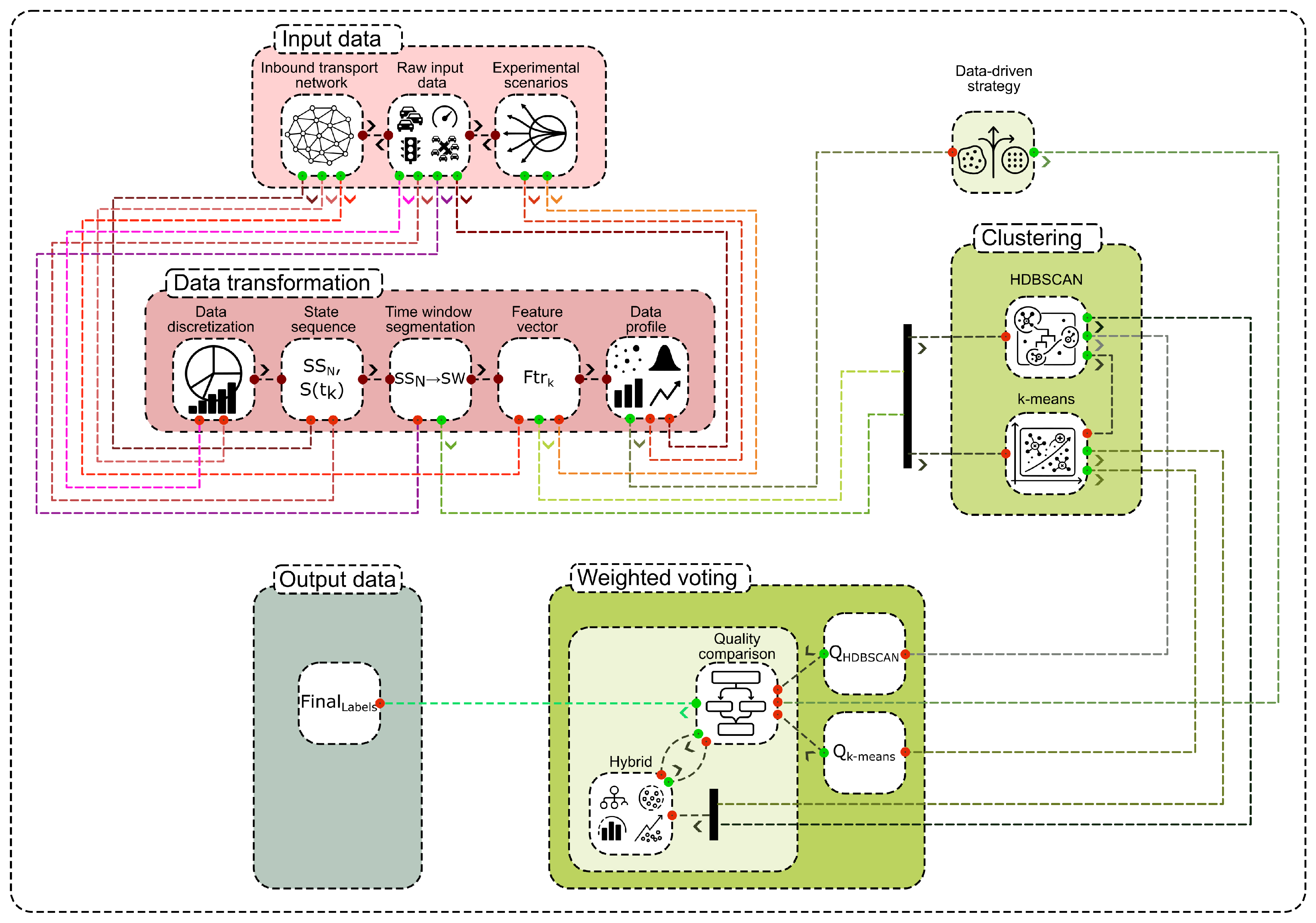
Figure 2.
Logical scheme of the weighted voting process. Input data characteristics, such as noise ratio and density variation, are evaluated to inform the selection between HDBSCAN and k-means. The quality of both models is assessed using internal and external metrics, and the final clustering result is chosen based on a comparative analysis, ensuring the most suitable model is applied.
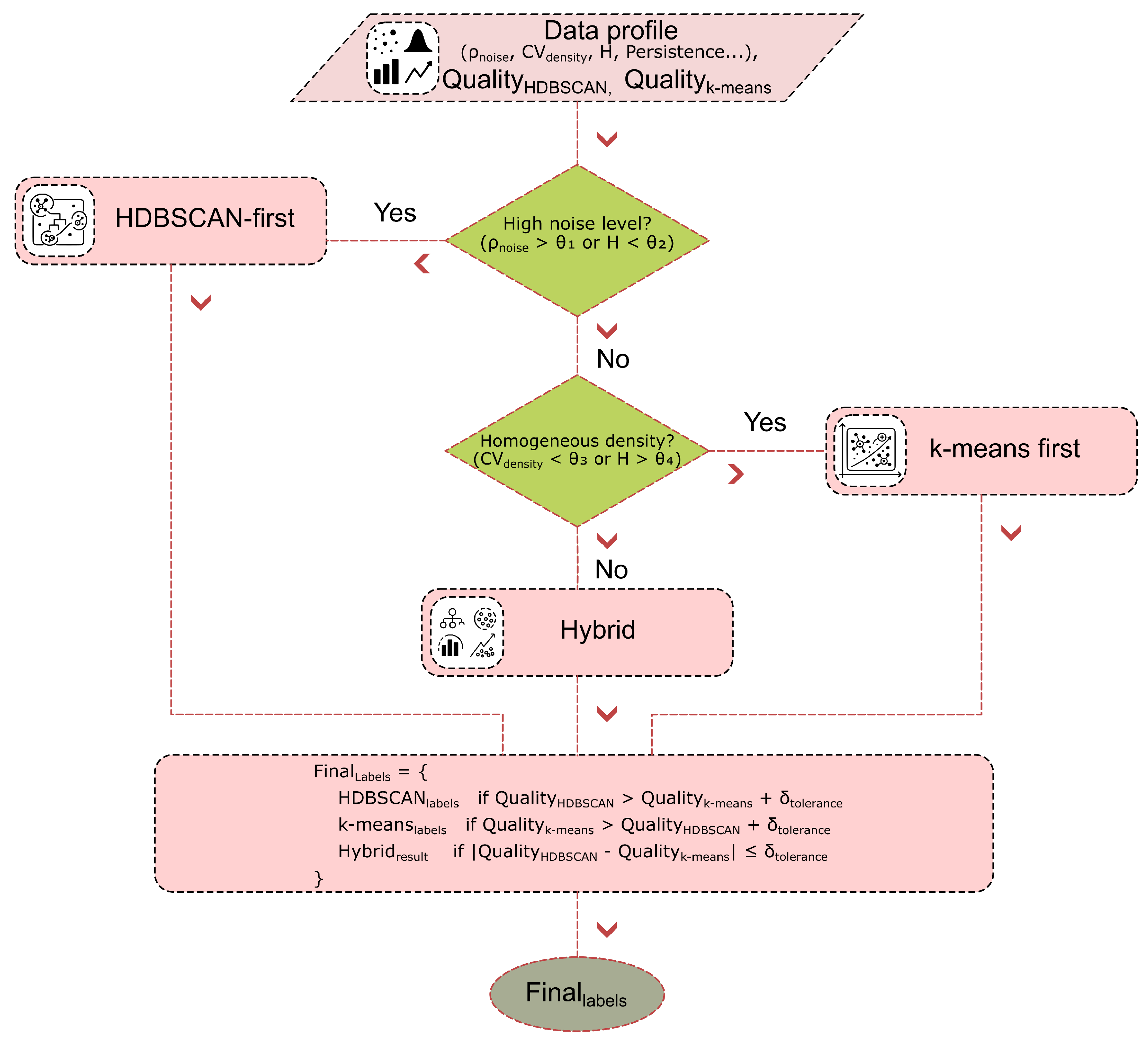
Figure 3.
Clustering of aggregated average traffic data using HDBSCAN. The algorithm automatically identified eight distinct clusters, effectively separating different simulated traffic modes and demonstrating a strong alignment with the ground-truth data structure.
Figure 3.
Clustering of aggregated average traffic data using HDBSCAN. The algorithm automatically identified eight distinct clusters, effectively separating different simulated traffic modes and demonstrating a strong alignment with the ground-truth data structure.
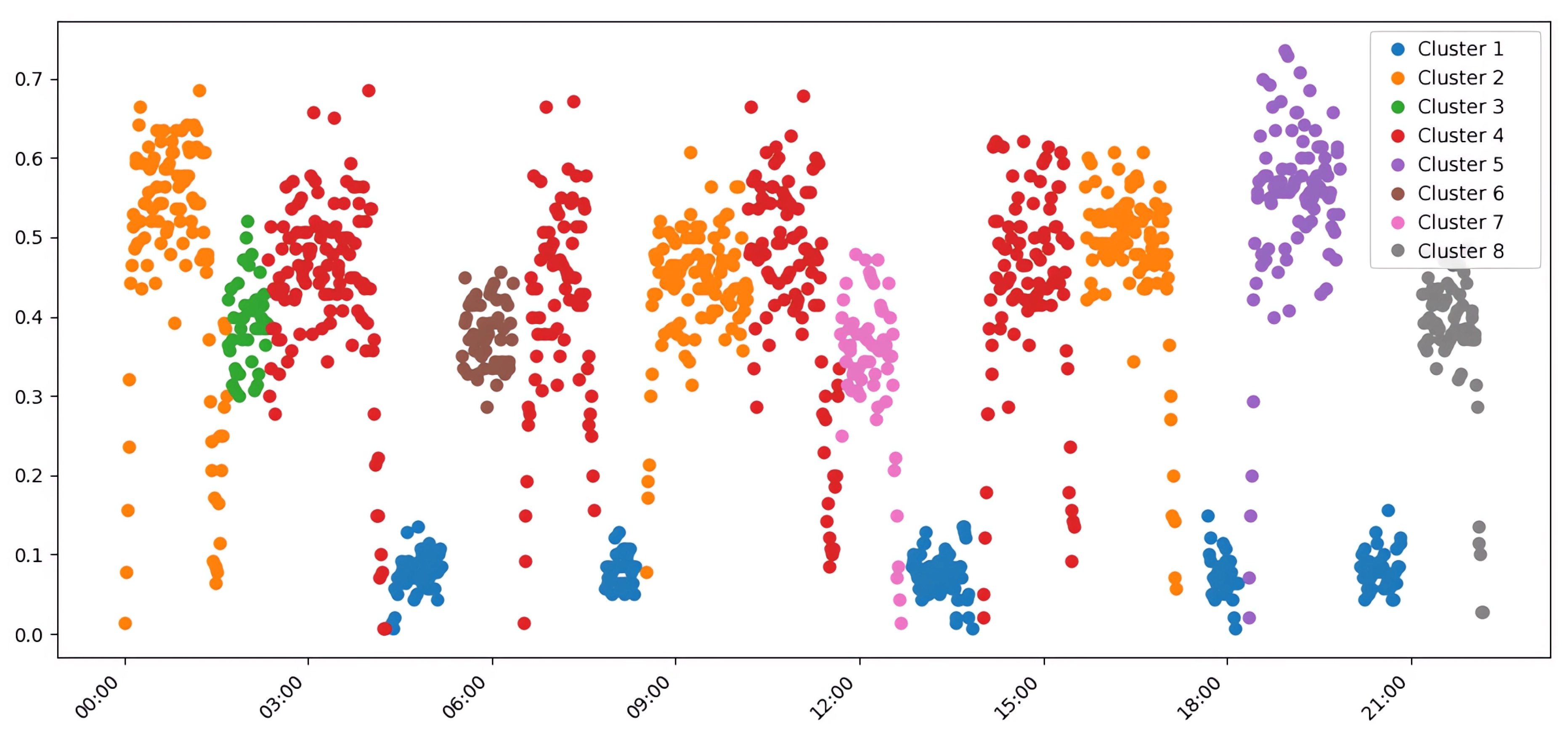
Figure 4.
Clustering of aggregated average traffic data using k-means with K=5. This approach produced compact, well-defined spherical clusters, leading to high internal validation scores, but merged some distinct traffic scenarios into single groups.
Figure 4.
Clustering of aggregated average traffic data using k-means with K=5. This approach produced compact, well-defined spherical clusters, leading to high internal validation scores, but merged some distinct traffic scenarios into single groups.
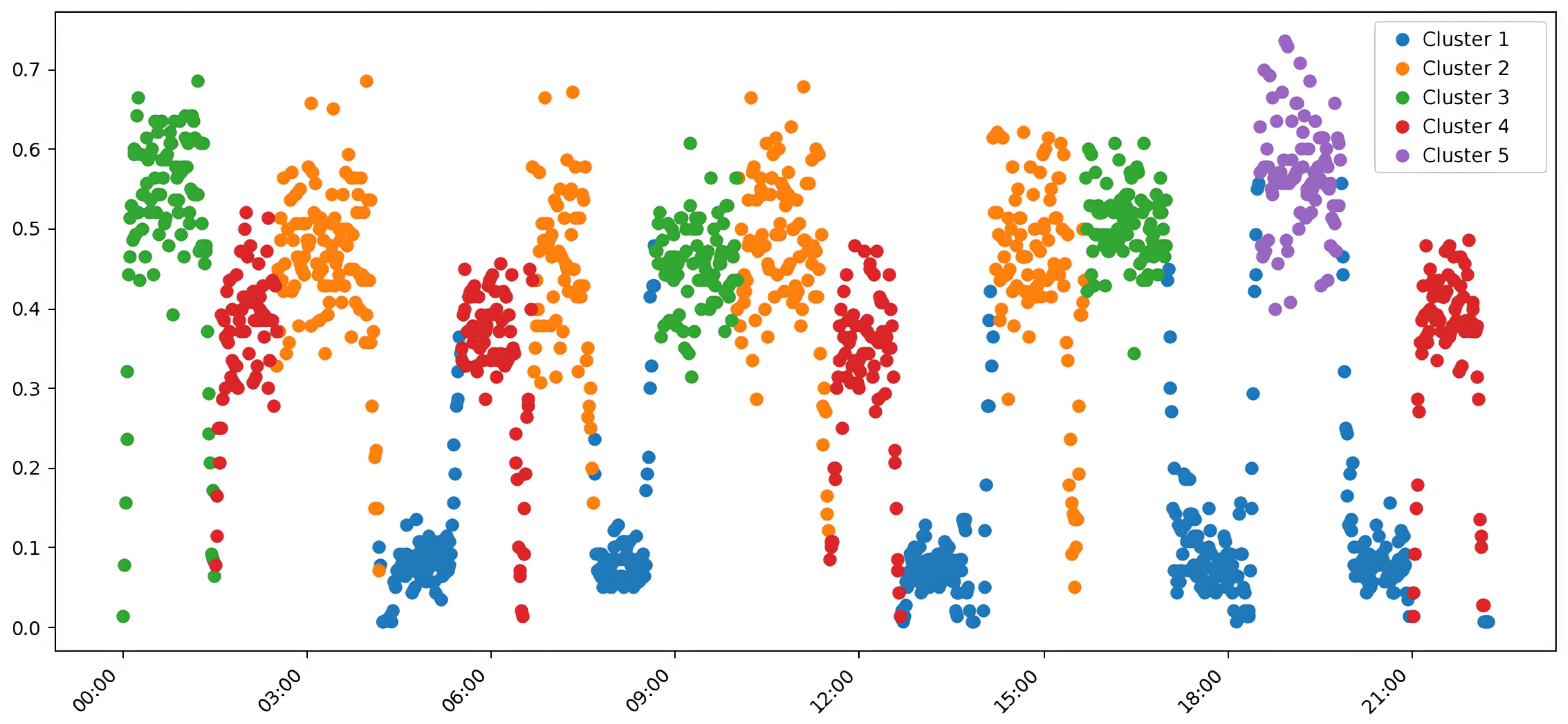
Figure 5.
Clustering of aggregated average traffic data using k-means with K=7. Increasing the cluster count resulted in over-detailing, where minor variations in traffic flow were incorrectly classified as separate patterns, reducing semantic clarity.
Figure 5.
Clustering of aggregated average traffic data using k-means with K=7. Increasing the cluster count resulted in over-detailing, where minor variations in traffic flow were incorrectly classified as separate patterns, reducing semantic clarity.
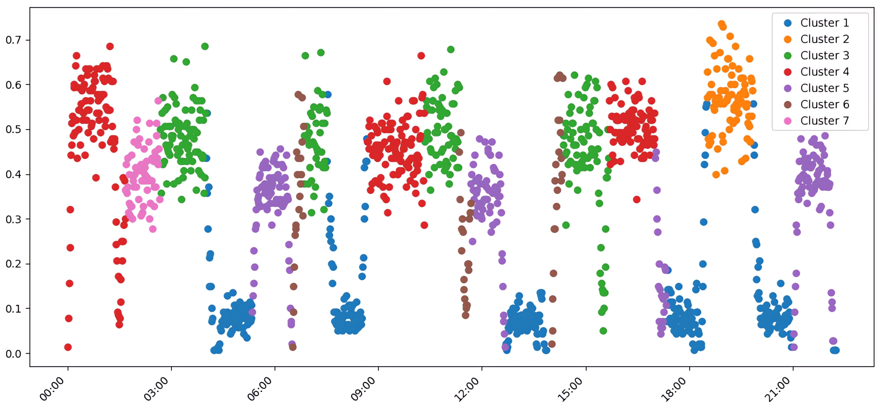
Figure 6.
Comparison of quality metrics for clustering approaches on aggregated average data. This chart highlights the trade-off between algorithms: HDBSCAN excels in external validation (V-measure, ARI), while k-means (K=5) performs better on internal metrics like the Silhouette Score.
Figure 6.
Comparison of quality metrics for clustering approaches on aggregated average data. This chart highlights the trade-off between algorithms: HDBSCAN excels in external validation (V-measure, ARI), while k-means (K=5) performs better on internal metrics like the Silhouette Score.
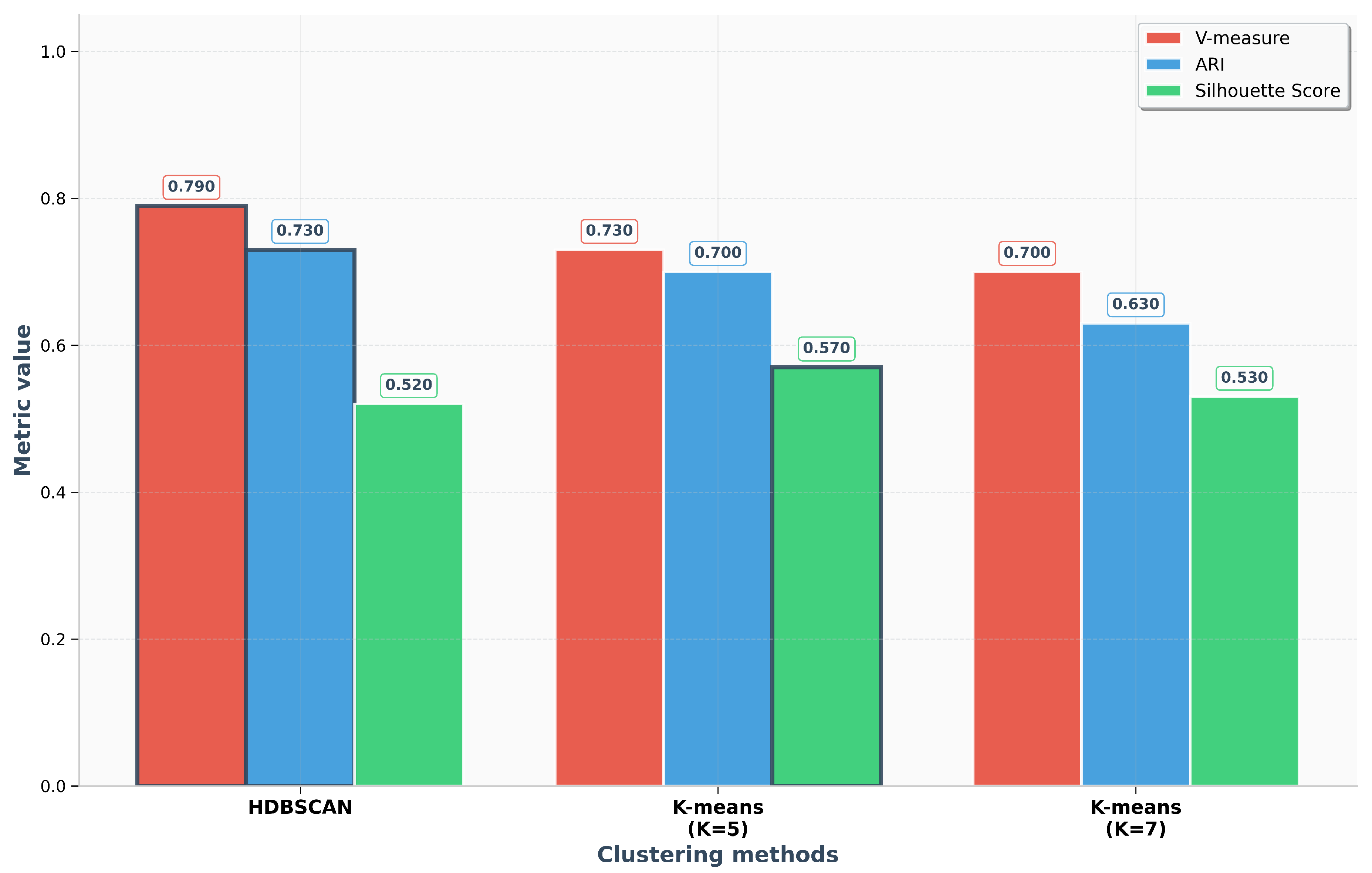
Figure 7.
Comparative analysis of clustering quality using V-measure and ARI metrics. The chart displays the performance of HDBSCAN, k-means (K=5), and k-means (K=7), illustrating that HDBSCAN is superior for lower-dimensional average data, while the performance gap narrows for high-dimensional data.
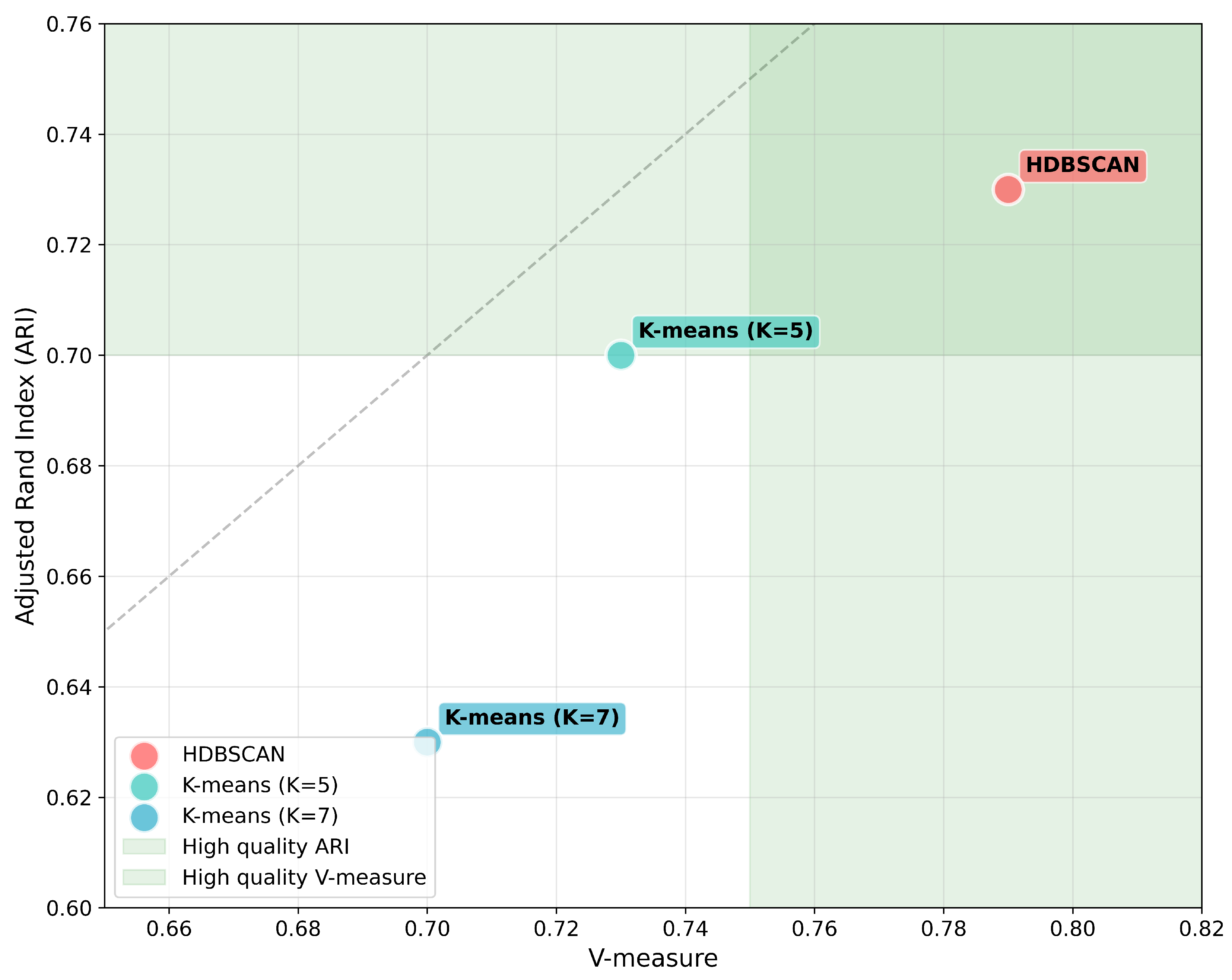
Figure 8.
Temporal distribution of transport scenarios and their corresponding cluster assignments by the HDBSCAN algorithm on aggregated average data. Each colored block represents a specific cluster, showing a clear, non-overlapping temporal sequence that aligns with distinct traffic patterns throughout the simulated day.
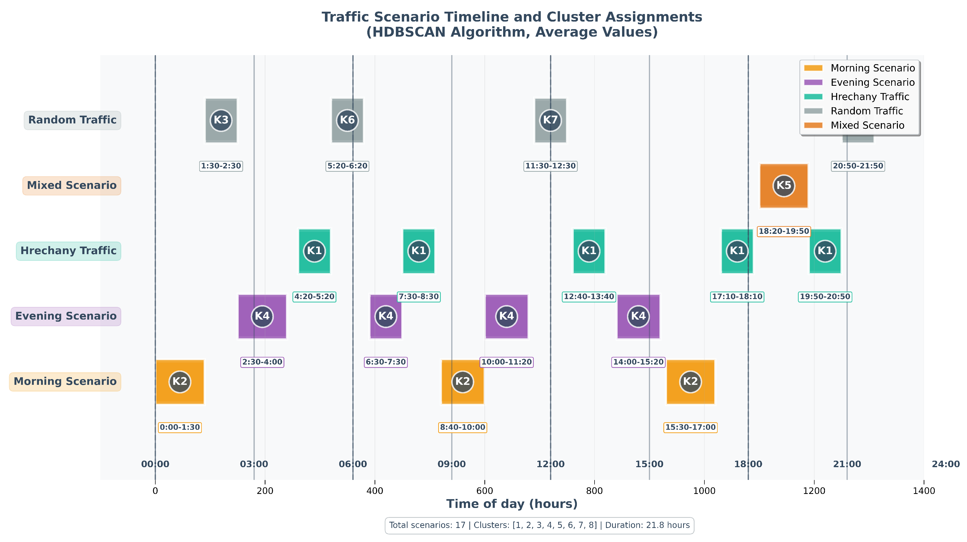
Figure 9.
Distribution of experimental scenarios within clusters identified by HDBSCAN on aggregated average data. (a) A bar chart detailing the number of scenarios per cluster, showing a balanced distribution. (b) A pie chart illustrating the proportion of each scenario type in the experiment, highlighting the five primary traffic modes: Hrechany, Evening, Random, Morning, and Mixed.
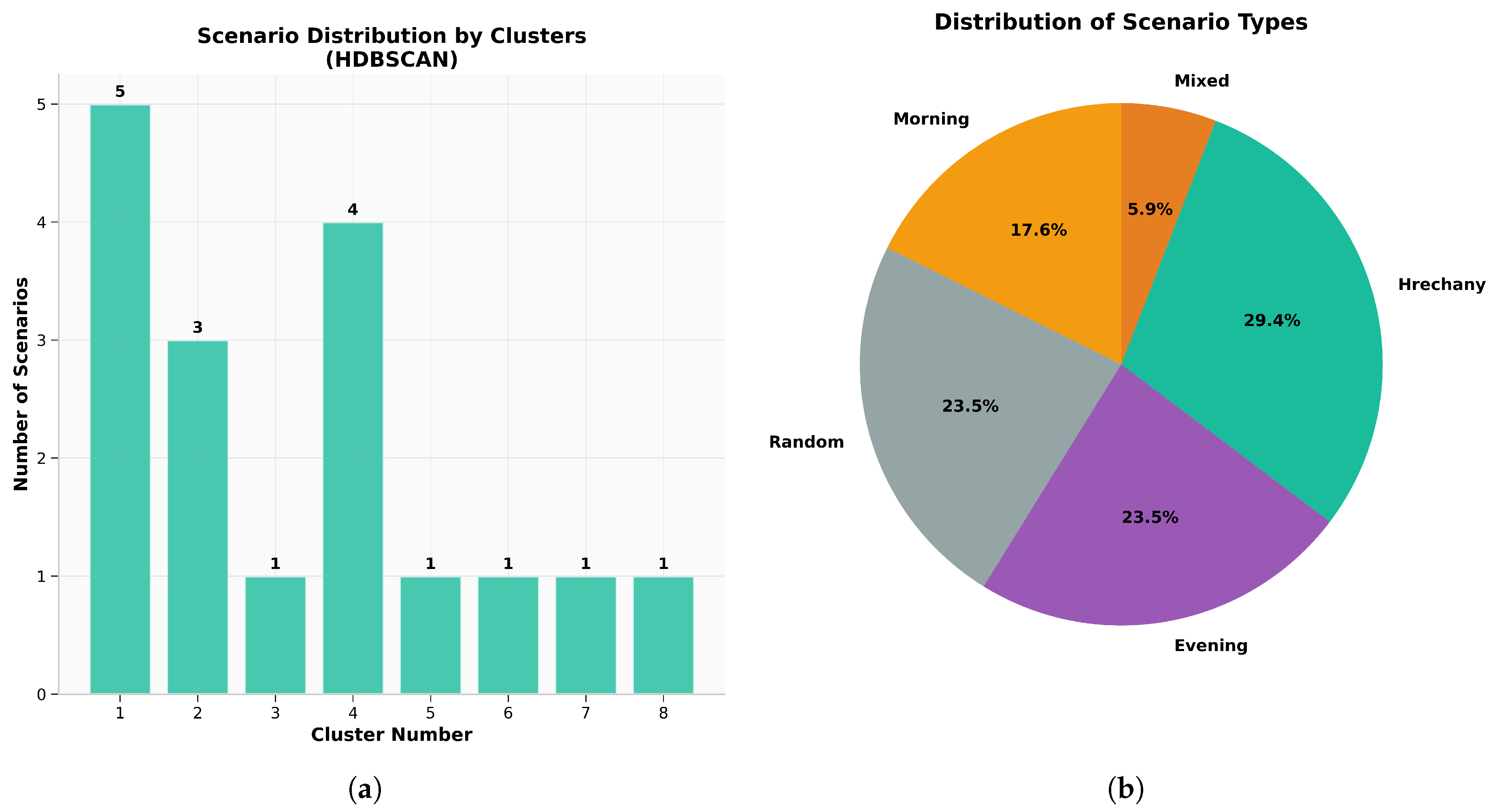
Table 1.
Clustering performance on aggregated average traffic data. External and internal validation metrics are presented for HDBSCAN, k-means (K=5), and k-means (K=7). Higher values are better for V-measure, Rand Index, ARI, NMI, Fowlkes–Mallows, Silhouette, and Calinski–Harabasz scores; lower is better for the Davies–Bouldin Index.
| Approach | V-measure | Rand Index | ARI | NMI | Fowlkes–Mallows | Silhouette | Calinski–Harabasz | Davies–Bouldin |
|---|---|---|---|---|---|---|---|---|
| HDBSCAN | 0.79 | 0.93 | 0.73 | 0.79 | 0.78 | 0.52 | 124.95 | 0.92 |
| k-means (K=5) | 0.73 | 0.90 | 0.70 | 0.73 | 0.76 | 0.57 | 292.23 | 0.65 |
| k-means (K=7) | 0.70 | 0.89 | 0.63 | 0.70 | 0.70 | 0.53 | 265.10 | 0.84 |
Table 2.
Clustering performance on high-dimensional combined traffic data. The table presents validation metrics for HDBSCAN and k-means, illustrating the impact of increased data dimensionality on algorithm performance.
Table 2.
Clustering performance on high-dimensional combined traffic data. The table presents validation metrics for HDBSCAN and k-means, illustrating the impact of increased data dimensionality on algorithm performance.
| Approach | V-measure | Rand Index | ARI | NMI | Fowlkes–Mallows | Silhouette | Calinski–Harabasz | Davies–Bouldin |
|---|---|---|---|---|---|---|---|---|
| HDBSCAN | 0.64 | 0.88 | 0.61 | 0.64 | 0.68 | 0.26 | 42.83 | 1.49 |
| k-means (K=5) | 0.67 | 0.87 | 0.62 | 0.67 | 0.71 | 0.23 | 34.79 | 1.59 |
| k-means (K=7) | 0.66 | 0.88 | 0.59 | 0.66 | 0.67 | 0.19 | 26.84 | 2.14 |
Table 3.
Comprehensive performance metrics for clustering algorithms on aggregated average traffic data. A full suite of external and internal validation metrics for HDBSCAN and k-means.
Table 3.
Comprehensive performance metrics for clustering algorithms on aggregated average traffic data. A full suite of external and internal validation metrics for HDBSCAN and k-means.
| Metric | HDBSCAN | k-means (K=5) | k-means (K=7) |
|---|---|---|---|
| V-measure | 0.79 | 0.73 | 0.70 |
| Rand Index | 0.93 | 0.90 | 0.89 |
| Adjusted Rand Index (ARI) | 0.73 | 0.70 | 0.63 |
| Mutual Information | 1.53 | 1.21 | 1.26 |
| Normalized Mutual Information (NMI) | 0.79 | 0.73 | 0.70 |
| Adjusted Mutual Information (AMI) | 0.75 | 0.70 | 0.67 |
| Fowlkes–Mallows scores | 0.78 | 0.76 | 0.70 |
| Silhouette Score | 0.52 | 0.57 | 0.53 |
| Davies–Bouldin Index | 0.92 | 0.65 | 0.84 |
| Calinski–Harabasz Index | 124.95 | 292.23 | 265.10 |
Table 4.
Comprehensive performance metrics for clustering algorithms on high-dimensional combined traffic data. The results illustrate the performance shift caused by the ’curse of dimensionality.
Table 4.
Comprehensive performance metrics for clustering algorithms on high-dimensional combined traffic data. The results illustrate the performance shift caused by the ’curse of dimensionality.
| Metric | HDBSCAN | k-means (K=5) | k-means (K=7) |
|---|---|---|---|
| V-measure | 0.64 | 0.67 | 0.66 |
| Rand Index | 0.88 | 0.87 | 0.88 |
| Adjusted Rand Index (ARI) | 0.61 | 0.62 | 0.59 |
| Normalized Mutual Information (NMI) | 0.64 | 0.67 | 0.66 |
| Adjusted Mutual Information (AMI) | 0.61 | 0.64 | 0.62 |
| Fowlkes–Mallows scores | 0.68 | 0.71 | 0.67 |
| Silhouette Score | 0.26 | 0.23 | 0.19 |
| Davies–Bouldin Index | 1.49 | 1.59 | 2.14 |
| Calinski–Harabasz Index | 42.83 | 34.79 | 26.84 |
Table 5.
Cluster assignments for key transport scenarios on aggregated average data. The table shows the categorization of different time periods and scenarios by the HDBSCAN, k-means (K=5), and k-means (K=7) algorithms.
Table 5.
Cluster assignments for key transport scenarios on aggregated average data. The table shows the categorization of different time periods and scenarios by the HDBSCAN, k-means (K=5), and k-means (K=7) algorithms.
| Time Period | Scenario Type | HDBSCAN | k-means (K=5) | k-means (K=7) |
|---|---|---|---|---|
| 00:00–01:30 | Morning | Cluster 2 | Cluster 3 | Cluster 4 |
| 01:30–02:30 | Random No. 1 | Cluster 3 | Cluster 4 | Cluster 7 |
| 02:30–04:00 | Evening | Cluster 4 | Cluster 2 | Cluster 3 |
| 04:20–05:20 | Hrechany | Cluster 1 | Cluster 1 | Cluster 1 |
| 05:20–06:20 | Random No. 2 | Cluster 6 | Cluster 4 | Cluster 5 |
| 06:30–07:30 | Evening (variation) | Cluster 4 | Cluster 2 | Cluster 6/3 |
| 07:30–08:30 | Hrechany (variation) | Cluster 1 | Cluster 1 | Cluster 1 |
Table 6.
Performance comparison between standalone algorithms and the cascade approach. The table showcases the improvements in clustering structure quality (V-measure) and compactness (Silhouette Score) achieved by the adaptive approach.
Table 6.
Performance comparison between standalone algorithms and the cascade approach. The table showcases the improvements in clustering structure quality (V-measure) and compactness (Silhouette Score) achieved by the adaptive approach.
| Criterion | HDBSCAN (Standalone) | k-means (Standalone) | Cascade Approach |
|---|---|---|---|
| Structure Quality (V-measure) | 0.79 | 0.73 | 0.79–0.82 (+0–4%) |
| Cluster Compactness | 0.52 | 0.57 | 0.57–0.59 (+4–13%) |
Table 7.
Scenario identification accuracy rates for different clustering approaches. The table shows the percentage accuracy for identifying five distinct transport scenarios and the average accuracy for each algorithm.
Table 7.
Scenario identification accuracy rates for different clustering approaches. The table shows the percentage accuracy for identifying five distinct transport scenarios and the average accuracy for each algorithm.
| Scenario Type | HDBSCAN (%) | k-means (K=5) (%) | k-means (K=7) (%) | Cascade Approach 1 (%) |
|---|---|---|---|---|
| Morning Peaks | 95 | 92 | 88 | 95–97 |
| Evening Peaks | 93 | 90 | 85 | 93–96 |
| Hrechany Scenario | 98 | 98 | 98 | 98 |
| Mixed Modes | 91 | 85 | 82 | 91–94 |
| Low-Active Periods | 87 | 83 | 79 | 87–90 |
| Average Accuracy | 92.8 | 89.6 | 86.4 | 92.8–95.0 |
1 Range reflects the selection of the optimal result for each scenario type.
Table 8.
Robustness of clustering algorithms to noise, measured by the ARI. The table shows quality degradation for each approach as Gaussian noise levels increase from 0% to 35%.
Table 8.
Robustness of clustering algorithms to noise, measured by the ARI. The table shows quality degradation for each approach as Gaussian noise levels increase from 0% to 35%.
| Noise Level | HDBSCAN | k-means (K=5) | k-means (K=7) | Cascade Approach 1 |
|---|---|---|---|---|
| 0% (basic) | 0.73 | 0.70 | 0.63 | 0.73 |
| 15% | 0.71 (–3%) | 0.64 (–8%) | 0.58 (–8%) | 0.71 (–3%) |
| 25% | 0.68 (–7%) | 0.60 (–15%) | 0.53 (–16%) | 0.68 (–7%) |
| 35% | 0.65 (–11%) | 0.55 (–21%) | 0.48 (–24%) | 0.65 (–11%) |
1 Based on preferred HDBSCAN selection at high noise level.
Table 9.
Temporal coherence analysis of clustering results. The table compares the temporal consistency of clusters generated by each approach, measured by a coherence coefficient and the number of temporal intersections.
Table 9.
Temporal coherence analysis of clustering results. The table compares the temporal consistency of clusters generated by each approach, measured by a coherence coefficient and the number of temporal intersections.
| Approach | Coherence Coefficient | Intersections in Time |
|---|---|---|
| HDBSCAN | 0.94 | 0 |
| k-means (K=5) | 0.89 | 2 |
| k-means (K=7) | 0.85 | 5 |
| Cascade Approach | 0.94 | 0 |
Table 10.
Statistical significance of performance differences (Wilcoxon signed-rank test). The table shows the W-statistic and p-value for key comparisons, confirming the significance of observed advantages.
Table 10.
Statistical significance of performance differences (Wilcoxon signed-rank test). The table shows the W-statistic and p-value for key comparisons, confirming the significance of observed advantages.
| Comparison | W-Statistic | p-Value |
|---|---|---|
| HDBSCAN vs. k-means (K=5) | 78 | 0.008 |
| HDBSCAN vs. k-means (K=7) | 85 | 0.003 |
| Averages vs. Combined Values | 92 | 0.002 |
Table 11.
Computational performance of the cascade approach on the experimental dataset (K=132 time windows, aggregated average data).
Table 11.
Computational performance of the cascade approach on the experimental dataset (K=132 time windows, aggregated average data).
| Processing Stage | Execution Time (seconds) |
|---|---|
| Feature Extraction | 1.48 |
| HDBSCAN Clustering | 4.72 |
| k-means Refinement (K=8) | 0.19 |
| Quality Evaluation and Voting | 0.45 |
| Total Runtime | 6.84 |
Disclaimer/Publisher’s Note: The statements, opinions and data contained in all publications are solely those of the individual author(s) and contributor(s) and not of MDPI and/or the editor(s). MDPI and/or the editor(s) disclaim responsibility for any injury to people or property resulting from any ideas, methods, instructions or products referred to in the content. |
© 2025 by the authors. Licensee MDPI, Basel, Switzerland. This article is an open access article distributed under the terms and conditions of the Creative Commons Attribution (CC BY) license (http://creativecommons.org/licenses/by/4.0/).
Copyright: This open access article is published under a Creative Commons CC BY 4.0 license, which permit the free download, distribution, and reuse, provided that the author and preprint are cited in any reuse.


