
Submitted:
02 August 2025
Posted:
04 August 2025
You are already at the latest version
Abstract
This review summarises potential applications of artificial intelligence (AI) in histopathological diagnostics of leukemias reported in the available literature. It compares existing AI models focused on analysing image-based cellular morphology, trained on datasets of either blood smears or bone marrow slides. Key findings indicate a rising trend in research output and literature on that topic, with models achieving high accuracy rates — up to over 95% in leukemia detection and subtype classification. The implications suggest that AI can significantly enhance diagnostic precision, reduce subjectivity, and streamline workflows in hematopathology. Possible limitations and difficulties of introducing AI to routine diagnostics are also elaborated on. Overall, integrating AI into leukemia diagnostics holds promise for improving early detection, supporting clinical decision-making, and advancing treatment in haematological malignancies.
Keywords:
hematopathology
; artificial intelligence
; leukemia
; histopathology
; diagnostics
1. Introduction
Today, an increasing emphasis on deep learning algorithms permeates all domains of human activity. In medicine AI-based decision aids are also gaining importance. The field in which computers could be an invaluable help for clinicians is the diagnosis of leukemias. Leukemias are among the 15 most common neoplastic diseases and in top 10 when it comes to mortality in 2024 according to WHO [1]. At the same time they are the most common neoplasms in the Polish pediatric population, accounting for 28, 7% of child tumors [2]. Only in 2024, in the USA 62000 new leukemia cases are expected to be diagnosed, of which will die [3]. During the last 30 years, a constant increase in cases has been observed (although with regional differences) [4]. Every diagnosis of leukemia must be confirmed by a pathologist with a microscope. Currently, ever more histological and cytological slides are scanned by specialized scanners and then stored digitally. This fact unlocks new possibilites for applying mechanical learning and using artificial intelligence to recognize abnormal cellular patterns. This narrative review explores application of this technology in leukemia diagnostics; it summarises and compares existing models and the data sets on which they are built, at the same time describing biases, challenges, and limitations that may hinder the spread of their use and the possible effects of their action on the final results of the diagnostic process.
2. Leukemias and Their Diagnostic Process
Hematopoiesis (the process in which cellular elements of human blood are created) in humans is very complex. While a detailed analysis and description of all stages and forms of cells development is outside the scope of this review, one has to note that normally, only final stages are represented in blood and intermediate forms are stored within the bone marrow [5]. The next paragraphs help to build understanding of the diagnostic process of leukemia and the complexities one has to understand to accomplish it. Leukemia is a neoplasm which derives from white blood hematopoietic cells and is caused by uncontrolled growth of one intermediate form in the hematopoietic chain. Rarely, it can be a normal, functional cell which due to mutation grows uncontrollably. An example of such leukemia can be leukemia introduced by HTLV-1 [6]. Such cells are not functioning properly and their growth causes suppression of other proper cells in blood. This leads to various symptoms, ranging from frequent infections to coagulation disorders. If untreated, symptoms may lead to death of the patient. General symptomatology of oncological disease (e.g fatigue, weight loss) often accompanies. Medical practitioners divide leukemias into 4 main types, depending on the cells that are overgrowing and on the rate of growth and disease dynamics: lymphoblastic leukemias (acute - ALL or chronic - CLL) and myeloid leukemias (acute - AML or chronic - CML) [7]. This classification is a simplification, since some leukemias are elusive and cannot be clearly ascribed to one type. There are many rare types of leukemia too, including hairy-cell leukemia (HCL) [8], prolymphocytic leukemia (PLL) [9], or large granular lymphocytic leukemia (LGLL) [10]. It is also possible for a mixed-phenotype leukemia to occur, where myeloid and lymphoid features are combined [11]. In order to be qualified to a type, leukemia must have a certain percentage of cancerous cells (e.g. >20% blasts in AML) or have defined cytogenetic abnormalities. If abnormalities occur, then the percentage of cells we have to establish the diagnosis of leukemia can either be smaller or doesn’t have importance at all for diagnosis. The aforementioned main types are further divided into subtypes - e.g. according to the French-American-British classification [12] (acute myeloid leukemia into subtypes M0-M7, or acute lymphoblastic leukemia into subtypes L1 - L3). The identification of the main type of leukemia is often insufficient and doctors need to know which exactly subtype they are to treat. The therapy differs between leukemia types and subtypes with some of them more threatening than others, mandating urgent response from the clinicians - a standard example of such subtype is acute promyelocytic leukemia (M3 subtype of AML according to FAB classification, where promyelocytes are the neoplastic cells) which causes life-threatening coagulation disorders (DIC) [13]. On the other hand, many chronic leukemias are indolent and patients sometimes for a long time don’t experience any symptoms. A good example of such leukemia is CLL, often diagnosed only after accidental discovery of lymphocytosis in patients’ blood [14]. A brief overview of leukemias, their markers and their diagnostic criteria are summarised in Table 1.
The diagnosis of leukemia can only be made by histopathological or cytopathological examination. Whereas histopathology is occupied with tissue samples, cytopathology analyses smears, where the intercellular structure is lost, and the cells are separated from each other. Both approaches provide important information and contribute to the final diagnosis [26]. Of course, the diagnosis of leukemia cannot be based solely on the morphological characteristics of cells under the microscope. Flow cytometry, immunohistochemical methods, and analysis of cell genotypes are used to support diagnosis [27]. Without them it would neither be possible to diagnose nor to treat leukemia. However, all these methods come after the morphological analysis, and the diagnostic process starts with histo- and cytology. The key step of this diagnostic process is also the one prone to most significant errors. The analysis of microscopic slides is done by eye and depends on the experience, expertise, and perceptivity of the analyst. The risk of errors is then high and unpredictable, and can reach 40% while differentiating between leukemia subtypes [28]. This fact does not imply that the diagnosis of the leukemia subtype is based solely on microscopy without employing other techniques that diminish the risk or error, but rather shows how subjective and difficult image analysis can be. While there is no diagnostic problem if e.g. there are 70% or 50% of blasts in AML specimen (we need 20% to be allowed to diagnose it), trouble begins if the amount is close to 20% - we cannot with certainty say if there are 19% or 21% of blasts… This is a field where an AI model trained to recognise leukemia cells, with its training and visual recognition capabilities far better than human, will immensely facilitate diagnostics.
3. Bibliometric Analysis
3.1. Bibliometric Analysis
In order to evaluate the current research trends and scientific interest in the application of artificial intelligence (AI) in histopathological diagnostics of leukemias, a bibliometric analysis was performed.
3.2. Methodology
Data source: Scopus
Time frame: 2018–2025 (as of July 12, 2025)
Keywords / Queries:
-
Q1: ("artificial intelligence" OR "AI" OR "machine learning" OR "deep learning") AND ("histopathology" OR "digital pathology" OR "histological image" OR "microscopic image") AND ("diagnosis" OR "diagnostic support" OR "classification")Broad general query covering applications of artificial intelligence in histopathological and cytological image analysis in hematology, without limiting to specific leukemia types.
-
Q2: ("artificial intelligence" OR "AI" OR "deep learning" OR "machine learning") AND ("leukemia" OR "leukaemia" OR "AML" OR "ALL" OR "CML" OR "CLL") AND ("diagnosis" OR "diagnostic aid" OR "detection" OR "classification") AND ("histopathology" OR "cytology" OR "microscopic image" OR "blood smear" OR "bone marrow smear")A more specific query targeting the use of machine learning and deep learning methods in leukemia diagnostics based on microscopic images, particularly focusing on blood and bone marrow cell morphology.
-
Q3: ("convolutional neural network" OR "CNN" OR "deep learning") AND ("blood smear" OR "bone marrow smear" OR "cytological image" OR "histopathology") AND ("leukemia" OR "blood cancer" OR "hematological malignancy")Query focusing on AI applications in automatic classification and detection of hematological diseases, with an emphasis on computer-aided diagnostic systems.
-
Q4: ("artificial intelligence" OR "machine learning") AND ("leukemia subtype" OR "ALL subtypes" OR "AML subtypes" OR "FAB classification" OR "immunophenotyping") AND ("classification" OR "differentiation" OR "subtype detection")Query focused on systematic reviews, meta-analyses, and review articles on the role of AI in leukemia diagnostics, capturing trends and current knowledge summaries.
-
Q5: ("machine learning" OR "deep learning") AND ("SVM" OR "support vector machine" OR "random forest" OR "CNN" OR "neural network") AND ("leukemia" OR "hematological malignancy") AND ("image analysis" OR "cell classification")Technical query covering innovative algorithms, neural network architectures (e.g., CNN), and explainable AI systems in morphological image analysis for hematologic diagnostics.
Inclusion criteria:
- Language: English
- Publication types: Articles, Reviews
- Topic: AI in histopathological/cytological diagnostics of leukemias
Screening protocol:
Three-stage abstract and title selection:
- 1.
-
From each publication set, we selected papers whose abstracts/titles contained at least one keyword from the:
- AI group (“artificial intelligence”, “ai”, “machine learning”, “deep learning”, “neural network”, “cnn”, “convolutional neural network”, “computer-aided diagnosis”, “automated diagnosis”, “intelligent system”)
- Morphological image analysis group (“histopathology”, “histopathological”, “cytology”, “cytological”, “microscopic image”, “blood smear”, “bone marrow”, “digital pathology”, “cell morphology”, “image analysis”)
- 2.
- From the publications passing the previous screening, we additionally selected only those where the abstracts/titles contained the word ”leukemia”.
- 3.
- Abstracts and titles of the selected publications were then analyzed, and those outside our thematic scope were excluded.
Deduplication: duplicate removal based on titles.
3.3. Results
The queries formulated and used in the Scopus database were characterized by high sensitivity but very low specificity. Designing more selective and complex queries carried the risk of omitting publications relevant to the topic of this study. As a result, thousands of publications were initially retrieved. From these, through the application of the triple-stage screening algorithm described earlier, several hundred articles were ultimately selected that reflect the scientific community’s interest in the subject of this review. While compiling the analysis, we took into consideration only such systems of artificial intelligence that work on images and carry out image analysis. We left outside the scope of our work models which analyse specific genetic mutations or chemical biomarkers and focused only on systems which analyse cellular morphology based on microscopic slides. The results of the analysis for each query are summarized as follows:
- Q1: 46,690 publications retrieved from Scopus → 10,939 after the first selection stage → 336 after the second selection stage
- Q2: 22,418 publications retrieved from Scopus → 4,438 after the first selection stage → 381 after the second fselection stage
- Q3: 2,397 publications retrieved from Scopus → 825 after the first selection stage → 299 after the second selection stage
- Q4: 1,780 publications retrieved from Scopus → 286 after the first selection stage → 147 after the second selection stage
- Q5: 2,646 publications retrieved from Scopus → 820 after the first selection stage → 255 after the second selection stage
After combining the publications from all queries and removing duplicates, a total of 430 articles were obtained. Following a detailed analysis of abstracts and titles, 12 articles were excluded as they were outside the scope of interest. This three-stage analysis enabled reliable filtering of several tens of thousands of publications, ultimately achieving a precision of 97.2%. However, this figure does not reflect the actual sensitivity, as the number of relevant articles potentially lost at the query stage remains unknown.
The data, shown in Figure 1, demonstrate a clear upward trend in the number of publications, peaking in 2024, indicating growing scientific interest in the application of AI in hematopathological diagnostics. Citation counts also show an increasing trajectory over time, with a distinct peak between 2021 and 2023, suggesting the emergence of influential articles shaping the development of this field. It is also interesting to see who are the main contributors by country - this is shown in Figure 2.
Institutional contributions are visualized in Figure 3, where the most active research centers are listed. Notably, several universities in Asia and the Middle East are among the top contributors, reflecting global academic interest beyond traditionally dominant regions.
A keyword co-occurrence analysis revealed common thematic foci across the included publications. Figure 4 presents the 15 most frequent keywords, with terms like “leukemia,” “machine learning,” “deep learning,” “bone marrow,” and “CNN” appearing most often. This suggests that most research is concentrated on the classification and segmentation of hematological images using modern deep learning techniques.
3.4. Limitations
This bibliometric analysis is based exclusively on data retrieved from the Scopus database, which may limit its comprehensiveness in capturing the global scientific output — particularly in comparison to other databases such as Web of Science or PubMed. However, the choice of Scopus was deliberate, due to its broad interdisciplinary coverage, high-quality metadata, export functionalities including citation data, and user-friendly analytical tools which enabled the implementation of complex filtering procedures. Furthermore, the analysis was conducted based on titles and abstracts without a full-text screening, which may have led to the omission of some relevant publications (false negatives) or the inclusion of articles only marginally related to the topic (false positives). The employed search algorithms relied on keyword matching, which increases the sensitivity of the analysis but may reduce its precision in the case of non-obvious formulations or interdisciplinary studies. Additionally, the citation counts were analyzed based on the data available at the time of extraction, meaning that these values are dynamic and may change over time.
3.5. Conclusions
This prepared bibliometric analysis demonstrates a clear increase in the number of publications addressing the application of artificial intelligence in histopathological diagnostics of leukemias in recent years, with a particularly notable acceleration observed between 2021 and 2024. This indicates a growing scientific interest in this research area and highlights the increasing importance of AI methodologies in hematological diagnostics. Furthermore, the analysis of keywords and article types reveals the predominance of studies focusing on deep learning methods, particularly convolutional neural networks, as well as the development of clinical decision support systems. The highest research activity is observed among institutions from China, India, the United States, and Saudi Arabia, reflecting the global and multi-center nature of work in this field. The affiliation analysis also shows that research is conducted both at large universities and smaller research centers, indicating widespread interest across various levels of the scientific community.
4. Datasets
This section offers overview of available databases for the developement and evaluation of medical image analysis models. In context of leukaemia diagnostics, these datasets offer annotated images that enable both training and benchmarking of AI-based diagnostic models. Table 2 summarises 43 such datasets related to leukaemia, detailing their publication year, number of images, resolution, magnification, diagnostic focus or task type, number of citations, and material source.
5. Image Processing Methods Used for Histopathological Diagnostics of Leukemias
In this paper, leukaemia detection is considered through image processing. Images are generally unstructured data, and their analysis is best done using deep learning models as opposed to classical models or expert-based AI [70]. Approches to image processing are commonly classified into two categories based on how the entire analytical process is structured:
-
Classical — staged or modular processing approach, whereby distinct phases can be identified:
- -
- preliminary processing (e.g., denoising, normalisation),
- -
- features extraction (e.g., segmantation, edge detection, Hough transform),
- -
- classification (e.g., SVM, random forest).
- End-to-End — final result is produced directly from raw data without any intermediate processing steps. Such processing can be carried out using Convolutional Neural Network (CNN) and its advanced variants, which includes models such as AlexNet, VGG16, ResNet, ResNeXt, and DenseNet.
Each metod contributes uniquely to the extraction and interpretation of relevant features from medical images, supporting acurate diagnosis. The following section provide a detailed overview of these techniques.
Segmentation — a division of pixels into mutually exclusive groups. A fundamental method of segmantation is thresholding, where pixels are assigned to classes based on a threshold T. Binarisation is a special case involving two classes. The basic form of binarisation is presented in equation (1), where pixel z is assigned to class 1 if its value is greather than or equal to the threshold T, and to class 0 otherwise.
A key aspect of thresholding is an appropriate threshold T selection. In many methods, this value is determined through histogram analysis. A comparative study of automatic threshold selection algorithms applied to image processing is presented in [71].
Hough Transform [72] — a technique developed to detect straight lines in images. It operates by mapping points from the Cartesian space into the Hough space. Equation (2) defines the perpendicular distance from the origin to a line forming an angle with the x-axis and passing through a point with Cartesian coordinates (x,y).
Typically Hough space is two-dimensional parameter space defined by the parameters and [73], where a single point in Hough space represents a straingt line in the Cartesian space. The transformation from Cartesian space to Hough space is a form of voting, where each point in the Cartesian space votes for the discrete set of lines passing through it. The number of votes corresponds to the numer of points lying on a given line. An extended version of the Hough transform have been proposed to the detection of the arbitrary shapes [74].
K-Nearest Neighbors (KNN) — a classification algorithm that does not involve a trainig phase. Instead, a reference dataset is simply stored in memory. This dataset is divided into classes (e.g., types of diagnoses). To classify a new instance, the distance (e.g., Eucidean distance) to the known reference cases is calculated. Then the class most commonly occuring among the k nearest neighbours is then assigned to the new instance.
Decision Tree (DT) — decision model operates as if–else conditions, which can be visualised as a tree composed of decision nodes. In the classical approach, each condition is based on a single feature. The construction of a decision tree begins with the entire training dataset. The feature that provides the most effective split is selected to form a logical condition (e.g., if blast cells > 20%), which partitions the dataset into subsets. Each resulting subset is then further divided based on the single feature that best separates the data at that level. This process is repeated recursively: features are selected, conditions are formulated, and new nodes are created until a stopping condition, such as reaching maximum tree depth or achieving a subset contains only one class. Each teaminal node (leaf) corresponds to a specific class and is used to assign a label to new instance [75].
Random Forest (RF) [76] — this method extends the concept of decision trees by combining the outputs of multiple independently constructed trees. Each tree is trained on a randomly selected bootstrap sample of the training data, and feature bagging is applied at each decision point by selecting a random subset of features. This double randomisation reduces variance and helps prevent overfitting. Trees are construced independently and in parallel, which makes the method computationally efficient and scalable.
Classification is performed by aggregation of all trees predictions. Typically through majority voting or probability averaging [76].
Gradient Boosting (GB) — a technique that builds multiple decision trees sequentially. In contrast to Random Forest, where trees are trained in parallel. In standard approach, each tree in GB is trained on the full training dataset with complete feature set. Successive trees aim to correct the prediction errors made by the ensemble. To reduce the risk of overfitting, GB typically uses shallow trees, with a maximum depth of 3 to 5 levels. Each indivitual tree is a weak learner and performs poorly in isolation, but their sequential combination yields a strong predictive model. Unlike Rndom Forest, where each tree independently predicts the final label, in Gradient Boosting each tree predict the gradient of the loss function with respect to the current prediction. These incremental updates are aggregated to form the final prediction.
The term Gradient Boosting reflects the core mechanism of the method:
- Gradient — each tree approximates the gradient of the loss function with respect to the current prediction.
- Boosting — combining many weak learners into a single strong model.
The optimisation procedure in Gradient Boosring is conceptually similar to Gradient Descent, commonly used to update weights in neural networks. However, instead of updating parameters directly, Gradient Boosting updates the model by adding new trees that reduce the overall loss in the direction opposite to the gradient [77].
Linear Regression — the method is based on fitting a linear combination of features x using weights w, expressed by the function (3), to the training dataset.
The prediction error for a single instance is calculated as the squared diffrence between the true value y and predicted value . The total error, denoted as loss function is defined as the mean of these squared errors over all training examples (4), and is commonly referred to as the Mean Squared Error (MSE). Coefficients w are determined by minimising loss function .
In machine learning, the symbol is commonly used to denote the predicted value, whereas y refers to the true value from trainig set. In the case of linear regression, the prediction is expressed as , as shown in equation (5).
Linear regression is applied to regression problems, where the output is a real-valued numer. Without additional modifications, the method is not suitable for classification tasks [75].
Logistic Regression (LR) — a method used for binary classification, where calsses are distinguished, e.g., ”leukemia” and ”non-leukemia”. The model predicts the probability of belonging to class 1, e.g., 95% probability of leukemia. It is based on a linear combination of features x, as shown in equation (5), similarly to linear regression. The result of linear combination (5) is then passed through the sigmoid function presented in equation (6).
Prediction in case of logistic regression is computed as sigmoid function applied to linear function , as shown in equation (7).
The value of function ranges from 0 to 1 and is used to represents the probability of belonging to calss 1. It predicts probabilities rather than continous values, making it suitable for classification tasks [78]. The loss in logistic regression , is calculated according to equation (8).
The model coefficients w are determined by minimizing the cost fuction from equation (8). Unlike linear regression, those coefficients cannot be obtained analitically. Instead, numerical methods such as Gradient Descent [75] or its variants, e.g., Momentum or Adam are used [79].
Regularisation — a technique used to prevent overfitting. It is typically achieved by incorporating a penalty term into the loss function, which discourages large weights values w. Consequently, the weights are kept close to zero. There are two common forms of regularisation used in linear models:
These regularisation techniques are widely adopted in machine learning models [75].
Ridge Regression — extension of linear regression that incorporates L2 regularisation [75,81], which penalises large coefficient calues w through (10). The Ridge Regression loss function presented in (11), augments the linear regression loss (4) with the L2 penalty term (10). The strength of the regularisation is controlled by the hyperparameter , which balances model fit and coefficient magnitude.
Ridge Classifier (RC) — classification approach based on Ridge Regression, defined by the loss function in equation (11). It is applied to binary problems with labels . The model fits a Ridge Regression, and prediction is made by thresholding the output function (3) as shown in equatin (12).
The threshold if 0.5 is used under the assumption that the classes are encoded as 0 and 1, and the model output is interpreted on this scale.
Lasso Regression (LR) — similar to Ridge Regression. The key difference is the use of L1 regularisation (9) instead of L2 [80]. The loss function for Lasso Regression is defined in equation (13). It combines the linear regression loss function (4) with the L1 regularisation (9). The strength of the regularisation is controlled by the hyperparameter .
Elastic Net — a combination of Lasso and Ridge Regression. It combines L1 regularisation (9) and L2 regularisation (10). The loss function (14) defined in equation (14) includes the hyperparameter controlling the regularisation L1 strength and controlling regularisation L2 strength. It enables the balance between feature selection and coefficient shrinkage [82].
Support Vector Machine (SVM) — a binary classification model trained on dataset , where , and . The model is based on a linear combination of features, analogous to the linear regression (3). Predictions are made based on the sign of the decision function, as shown in equation (15). The output is eiter or .
The training objective is to maximise the separation between two classes and . It is done by increasing the margin, defined as the distance between the decision boundary and the nearest data points. A larger margin is assumed to improve generalisation of the model to new data. It has been observed that the classification boundary is determined by a small subset of the training data, known as support vectors [83], which lie closest to the margin.
SVM uses the hinge loss function , defined in equation (16), which penalises misclassifications and margin violations. Only examples within a margin of 1 contribute to the loss.
The overall loss function consists of two components: a regularisation term and the hinge loss, as shown abstractly in equation (17). Typically, L2 regularisation is employed.
To control the trade-off between model complexity and classification performance, different scaling strategies for the loss function are used. In the original formulation [83], the hinge loss is scaled by hyperparameter C, as shown i equation (18). Note that the regularisation term (10) is scaled by for convenience, resulting in gradient of w rather than .
An alternative formulation has been proposed in [75], where the regularisation term (10) is scaled by , and the hinge loss is averaged over all treining samples. This approach is shown in equation (19).
Both (18) and (19) allow one to control the balance between regularisation and the hinge loss, but they achieve this through different scaling mechanisms.
k-means This clustering — algorithm partitions data into k disjoint groups called clusters. The number of clusters k is defined prior to training. The clustering is performed by minimising the within-cluster sum of squares (WCSS), i.e., the sum of squared Euclidean distances between data points x and their assigned cluster centroids . The loss function is formally definied in equation (20). It aggregates the squared distance between each of the n data points x and the centroids of the cluster to which it is assigned. The set denotes all data points x assigned to cluster j. The corresponding cluster centroid is denoted by .
The k-means minimise the loss function by iteratively refining the assignment of data points x and the positions cluster centroids . At each iteration the algorithm performs two alternating steps:
- 1.
- Assignment step — each data point is assigned to the cluster whose centroid is closest.
- 2.
- Update step — for each cluster , the centroid is updated as the mean of the data points assigned to cluster , as show in equation (21).
These two steps are repeating until convergence, typically when cluster assignments stabilise or the decrease in falls below a set threshold [84].
Multilayer perceptron (MLP) — a feedforward artificial neural network (ANN) composed of layers of units called neurons. The network consists of an input layer, one or more hidden layers, and an output layer producing the prediction . Each neuron computes a linear combination of its inputs, analogous to the linear function defined in equation (3). Specifically, in layer l, neuron j computes linear combination of its weights and the outputs of neurons from previous layer, denotes as , as shown in equation (22).
The output of the neuron j on layer l is then computed by applying a nonlinear activation fuction to the linear combination . This output is defined as in the equation (23).
Logistic regression can be interpreted as a single-neuron MLP with sigmoid (6) activation, whose schematic is shown in Figure A1. The diagram illustrates the linear combination of inputs and weights represented as a circle, followed by the sigmoid activation function shown as a rectangle, producing the output prediction .
MLP generalises this concept by stacking multiple neurons into layers with various activation functions. In a standard MLP, each neuron in a given layer receives as input all outputs from the neurons in the precending layer. This type of connection is reffered to as a fully connected (FC) or dense layer [75]. A schematic of such a network is presented in Figure A2. It consists of a single input layer with 5 inputs, denotes as . There are two hidden layers, each containing 3 neurons. The first hidden layer inlcludes neurons , and the second hidden layer includes neurons . Finally, there is a single output .
Convolutional Neural Network (CNN) — an artificial neural network architecture specifically designed for image processing tasks. A foundational contribution in this area is LeNet-5 architectur introduced in [85]. In [85], convolutional layers were proposed to enable the local extraction of features such as edges, corners, textures etc. without the need for manual feature engineering. The mathematical formulation of a convolutional layer is presented in equation (24), where X denotes the input to the layer, K is the convolutional kernel, b is the bias term, is the activation function, and Y represents the output of the layer.
The operation reffered to as convolution (25) in equations (24) is, in fact, a cross-correlation, as the kernel K is not flipped as in the strict mathematical definition. Nevertheless, this operation is convencionally called convolution and will be reffered to as such throughout this paper.
The convolution (in practice, cross-correlation) of an input matrix X with a filter K of size produces an output matrix Z. Each element is computed as the sum of element-wise products between the overlapping region of X and the filter K, as shown in equation (26).
This operation (26) is performed by sliding the filter K across the spatial dimensions of X. At each location, local patch is combined with the filter, and the result forms a single output value.
When the input matrix X is a two-dimensional array, as in (26), it can be interpreted as a single-channel image (e.g., a grayscale image). In the multi-channel case, such as RGB image, the filter is extended across channels. The output is then computed as the sum over all d channels, as expressed in equation (27).
A common application of convolution prior to its use in CNNs was edge detection, using fixed kernels such as the Roberts [86], Sobel [87] and Prewitt [88] operators. The Sobel operator [87] consists of two filters: and , shown in equation (28). The first filer, , detects vertical edges, by responding strongly to horisontal intensity changes. The second filer, , detects horisontal edges, by responding strongly to vertical intensity changes.
In contrast to these manually designed edges detectors, the filters in CNNs are not predefined. Instead they are represented by trainable weights w which are learned from data during training.
In classical CNN architectures, convolutional layers are typically followed by pooling layers. In the original LeNet-5 architecture [85], there were referred to as subsampling. Althrough the term pooling is now more widely used. A pooling layer operates similarly to a convolutional layer, sliding a fixed size window (e.g., ) over the input matrix. However, instead of computing a weighted sum, it applies an aggregation function. Common choices includes the maximum (max pooling) or the average (average pooling). Pooling layers do not contain trainable parameters. Their behaviour remains fixed during both training and evaluation.
The convolutional and pooling layers produces a multi-dimensional feature map, typically represented as 3D matrix. To enable classification, this feature map is flattened into a one-dimensional vector by a dedicated flatten layer. The flattened representation is then passed to a fully connected network, structurally identical to a traditional multilayer perceptron (MLP). These layers generate the final prediction, such as a classification. A schematic overview of the LeNet-5 is presented in Figure A3.
AlexNet — a Deep Convolutional Neural Network (DCNN) proposed in [89], which achieved first place in the ImageNet ILSVRC-2012 competition. The AlexNet architecture represents an extension of the classical LeNet-5 approach. A schematic overview of the AlexNet is presented in Figure A4. This networks consists of five convolutional layers, each followed by ReLU activation function. After the first convolutional layer, response normalisation [89] and max pooling are applied. The same sequence follows the second convolutional layer. The third, fourth, and fifth convolutional layers are applied consecutively without intermediate layers. Max pooling is applied only after the fifth convolutional layer. The output from this max pooling is passed to a flatten layer, which reshapes the feature map from a matrix into one-dimensional vector of size 9216. This vector is then fed into three fully connecded layers. The first two uses ReLU activation, while the final layer consists of 1000 neurons with softmax activation, corresponding to the 1000 target classification categories.
VGG16 — a deep convolutional neural network (DCNN) proposed by Simonyan and Zisserman from the Visual Geometry Group (VGG) at the University of Oxford [90]. In their work, six model variations were introduced, differing in number of parameters and depth of 11, 13, 16 and 19 layers.
The architecture employs convolutional layers with filters and same padding, ensuring that the spatial dimensions of the input and output feature maps remain identical. These convolutional layers are grouped into blocks. Each block contains two to four consecutive layers followed by max pooling layer. An example of such a module, containing three convolutional and single max pooling layer is shown in Figure A5.
The standard VGG network [90] is composed of five such blocks, each with a varing number of convolutional layers, followed by three fully connected (FC) layers at the end. The final layer consists of 1000 neurons with softmax activation, identical to the output configuration used in AlexNet [89]. The term VGG16 refers to the version with a total of 16 learnable layers: 13 convolutional and 3 fully connected layers. The convolutional layers are distributed across the five blocks as follows: 2, 2, 3, 3 and 3.
ResNet — a deep convolutional neural network (DCNN) architecture introduced in [91]. Its’ key innovation is the introduction of skip connections which create a direct pathway between the input and output of a block. An example of such a block i shown in Figure A6 where the input x is passed through two convolutional layers, Conv1 and Conv2, producing an intemediate output . The input x is then added to this output, resulting in , followed by a ReLU activation.
These skip connections allows the network to skip certain layers through residual learning, thereby improving gradient propagation. It effectively addresses the vanishing gradient problem and enables training of very deep networks. In [91], authors evaluated architectures from 20 do 1202 layers. In practice, commonly used ResNet variants include ResNet-18, ResNet-34, ResNet-50, ResNet-101 and ResNet-152.
ResNeXt — an extension of the ResNet architecture was proposed in [92]. Its key component is a transformation block which incorporates multiple parallel convolutional paths. A schematic representation of a typical ResNeXt block is presented in Figure A7. Each path, also reffered to as a cardinality branch, processes the input x independently using sequence of convolutional layers. The number of paths is defined by a hyperparameter known as cardinality [92]. The usual configuration of each path includes three convolutional layers per path: , and . While the structure of these paths is identical, each utilises separate, independently learned weights. The outputs of all paths are summed element-wide. This is then combined with the original input x via a skip connection, following the residual learning approach introduced in ResNet.
DenseNet — a deep convolutional neural network (DCNN) architecture introduced in [93]. Its key innovation lies in the introduction of dense connections, which extend the concept of skip connections originally proposed in ResNet [91]. In DenseNet, each layer receives as input a concatenation of the outputs from all preceding layers, rather than just from the immediate previous one. Each layer produces a fixed number of new feature channels, referred to as the growth rate, which are appended to the existing feature set. As a result, the number of channels increases linearly with network depth. To reduce feature dimensionality, between dense blocks are inserted transition layers, consisting of convolution followed by pooling layer.
Inception — a deep convolutional neural network (DCNN) architecture proposed in [94]. Its key feature is the use of parallel processing within an Inception module where each path performs a different operation. The structure of a single Inception module is shown in Figure A8. This module contains four parallel branches, all of which receives the same input x:
- a sequence of followed by convolutions,
- a sequence of followed by convolutions,
- a max pooling followed by convolution,
- a single convolution.
- The outputs of all paths are concatenated along the channel dimension.
Inception combines the idea of multi-branch parallel processing from ResNetXt with the feature aggregation characteristic of DenseNet. However, unlike ResNet and DenseNet, Inception does not use skip connections.
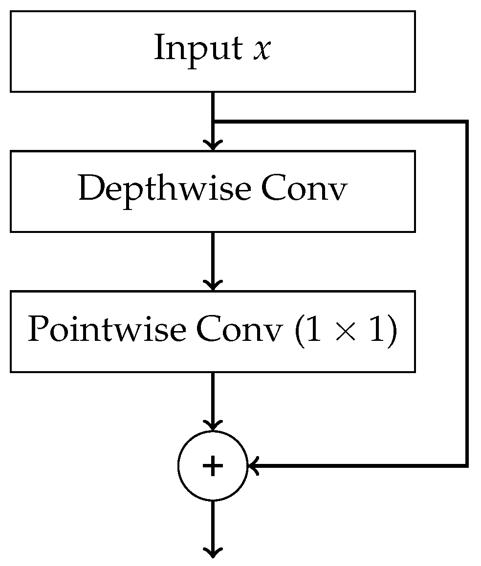
Xception — a deep convolutional neural network (DCNN) architecture proposed in [95], which extends the concept introduced in Inception. Its core innovation is the use of depthwise separable convolutions. The structure of a single Xception block is shown in Figure A9. In the main processing path, a depthwise convolution is first applied. It is a spatial convolution performed independently on each input channel. This is followed by a pointwise convolution , which combines the output channels. Additionally, skip connections are employed between blocks, in a manner similar to ResNet.
Xception extends the Inception architecture by using depthwise separable convolutions which generalize the parallel convolutional paths used in Inception. It also incorporates skip connections, as introduced in ResNet.
The presented methods are widely applied in the histopathological diagnosis of leukaemias. A summary of selected scientific publications demonstrating the practical application of these methods is provided in Table 3.
6. Discussion on Biases and Limiations of AI Used in Histopathology
The diagnostic process in pathology is a certain sequence of events that need to occur before we are able to reach diagnosis. The tissue samples need to be collected, processed, fixated, transported onto slides and stained before we can watch them under our microscope [106]. These steps are necessary, but they also introduce errors (artifacts) in our slides, making their interpretation harder [107]. If we were to apply digital solutions, the process must also include scanning the slides so that they can be stored on computer and analysed by it. The scanning needs to keep the resolution good, the colours sufficiently preserved and the technical parameters of scanning device need to be of good quality. There is a wide selection of such scanning devices in the market [108], but their price might be a serious obstacle to availability of AI-related diagnostic technologies in smaller/poorly funded laboratories. While scanning, we cannot remove or correct the slides as to get rid of artifacts - they are all preserved on scanned image [109], making it analysis by AI harder. The resolution and magnification of slides undergoes changes when the slide is scanned and displayed on monitor rather than under the microscope [110]. Difference in resolution might mean that some tiny, yet diagnostically important parts of the slide might no longer be seen on the slide version seen by the AI. Another diagnostic problem is that some tissue samples are only small pieces (biopsies) or are fragmented and their architecture is lost (e.g. many polyps obtained by endoscopy arrive fragmented) - fragmentation is another challenge which AI would have to overcome. While tissue fragmentation is not a problem in cytological specimen this phenomenon has utmost importance while diagnosing solid tumours or e.g. lymphomas.
The AI models do not guarantee 100% perfection. An old Polish saying goes "only those who don’t do, don’t err". In medicine, errors are an unavoidable part of medical practice in every specialisation including pathology. The sources of errors in diagnostics can be multifarious, including swapping the specimens or wrong storage/preparation [111]. Some of the errors are a consqeuence of simple clerical errors like mislabelling the slides [112]. Unfortunately, some wrong diagnoses are inevitably on the pathologists side. A study by Packer et al. [113] found out that from 134 analysed cases, 37 (27,6 %) were diagnosed with a wrong entity. Nevertheless, trained pathologists can reach very high rates of success. A study by Dehan et al. [114] showed a remarkable rate of correct diagnoses in frozen intraoperative specimens (which due to their processing abound in artifacts and are more difficult for a pathologist to diagnose) - only 2,9 percent of errors in over 6000 samples. The use of artificial intelligence in diagnosing of leukemias brought similar rates of success, with some models [63,65,66] reaching similar rates of accuracy in answering the given problem.
Even after a successful diagnosis in spite of the aforementioned error sources has been reached, not all problems are solved. According to the law, all pathology specimens need to be stored for a fixed amount of time to ensure the possibility of reviewing the diagnosis or solving eventual claims and disputes. In Poland, this obligatory storage period is 10 years in case of cytological specimens and 20 years in case of histopathology specimens [115]. The same requirement would obviuosly concern samples in virtual/digital form. If we realize that a single slide scanned occupies from 1 to 3 GBs [116], many cases consist of multiple slides from the same patient, and the demand for histopatological examinations is on the rise [117], one can easily imagine how high storage ability would be required from the laboratories to store all required by law data for such a long period. Such a large amount of data requires a lot of time to scan it - some slides may require 1000 seconds to be scanned [116].
Potential benefits of applying deep learning technologies in pathology are not limited to leukemias. A lot of models were already created for AI to help diagnosing kidney pathologies [118], colorectal cancer [119], and prostate cancer [120]. Some of the models reached good results enough to be approved by relevant regulatory authorities (e.g. FDA in case of the United States) and can be routinely employed to diagnose patients, the first of such algorithms accepted in 2021 [120]. Currently, the list of AI-based solutions approved by FDA in various domains of medicine has 1247 entries; over 900 of them are from radiology domain, with haematology having 19 entries and pathology 6 [121]. Since radiology is predominantly image analysis, technologies connected to it (similar to those presented in our review) are dominating the market of medical services. It seems that pathology, with only 6 registered entries up to date still has many potential solutions to develop yet.
A serious limitation of all AI-based models is that they cannot solve problems other than those for which they were created. Where a human pathologist can effortlessly switch between diagnosing cases from different systems of the human body in just a few minutes, such a change in case of AI would require creating an entirely new model or a lot of training. Before fully replacing humans, AI would also need to learn integrating information from different diagnostic methods (flow cytometry, genetic methods), ordering and interpreting additional immunohistochemistry staining and keeping eyes open for artifacts and dust which often distort the image to be seen on slides. Pathology cannot be reduced to black-white IT-like binary distinctions - it is the ability to see all shades of grey in between that enables us to reach accurate diagnoses. Time leaves open the question, whether AI will ever be able to supplant human pathologists and, if yes, when will this happen.
Author Contributions
Conceptualization, M.C.; methodology, G.R., A.Ż., P.K., M.C.; software, P.K., P.T., A.S.; validation, M.C., P.K.; formal analysis, M.C., P.K., P.T., G.R., A.Z., A.S.; investigation, M.C., P.K., P.T., G.R., A.Z., A.S.; resources, M.C., P.K., P.T., G.R., A.Z., A.S.; data curation, M.C., P.K., P.T., G.R., A.Z., A.S.; writing—original draft preparation, M.C., P.K., A.S., P.T., G.R., A.Ż.; writing—review and editing, M.C., P.K., A.S., P.T., G.R., A.Ż; visualization, P.K., A.S.; supervision, G.R., A.Ż.; project administration, M.C., G.R., P.K.. All authors have read and agreed to the published version of the manuscript.
Funding
This research received no external funding.
Institutional Review Board Statement
Not applicable.
Informed Consent Statement
Not applicable.
Data Availability Statement
Since the article is a narrative review, no new data were created during our work on this article; thus data availability doesn’t apply here.
Acknowledgments
Not applicable.
Conflicts of Interest
The authors declare no conflicts of interest.
Abbreviations
The following abbreviations are used in this manuscript:
| WHO | World Health Organisation |
| AI | Artificial Intelligence |
| HTLV-1 | Human T-cell Lymphotropic Virus type 1 |
| ALL | Acute Lymphoblastic Leukemia |
| AML | Acute Myeloid Leukemia |
| CLL | Chronic Lymphocytic Leukemia |
| CML | Chronic Myeloid Leukemia |
| HCL | Hairy-Cell Leukemia |
| PLL | Prolymphocytic Leukemia |
| LGLL | Large Granular Lymphocytic Leukemia |
| MPAL | Mixed-phenotype Acute Leukemia |
| MM | Multiple Myeloma |
| FAB | French-American-British Classification |
| DIC | Disseminated Intravascular Coagulation |
| KNN | k-Nearest Neighbour |
| DT | Decision Tree |
| RF | Random Forest |
| GB | Gradient Boosting |
| LR | Logistic Regression |
| SVM | Support Vector Machine |
| RC | Ridge Classifier |
| MLP | Multilayer Perception |
| ANN | Artificial Neural Network |
| FC | Fully Connected |
| CNN | Convolutional Neural Network |
| DCNN | Deep Convolutional Neural Network |
| WCSS | Within-Cluster Sum of Squares |
| FPR | False Positive Rate |
| FNR | False Negative Rate |
| FDA | Food and Drugs Administration |
| VGG | Visual Geometry Group |
Appendix A
Figure A1.
A schematic diagram of the single neuron in MLP.
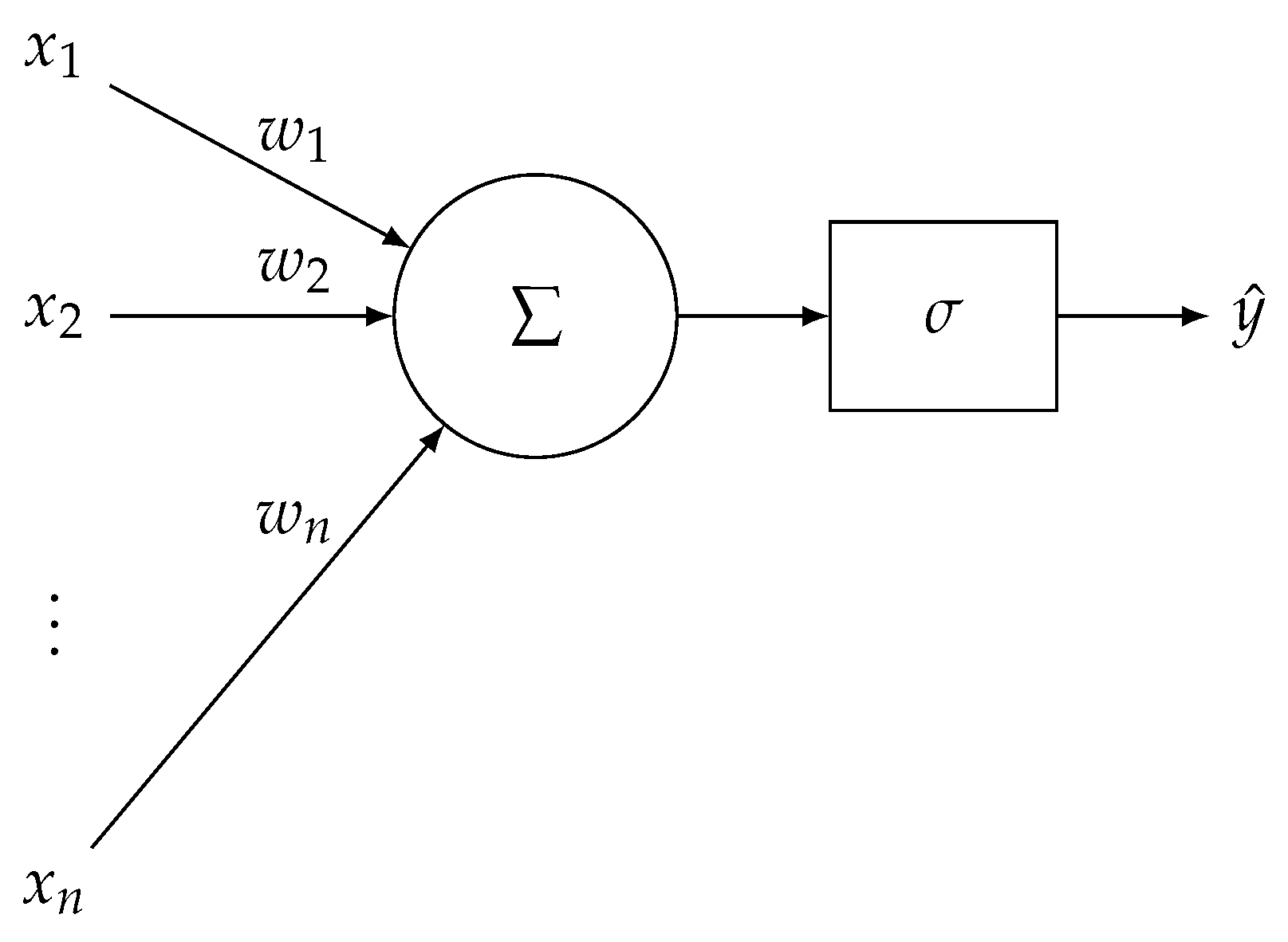
Figure A2.
A schematic diagram of MLP.
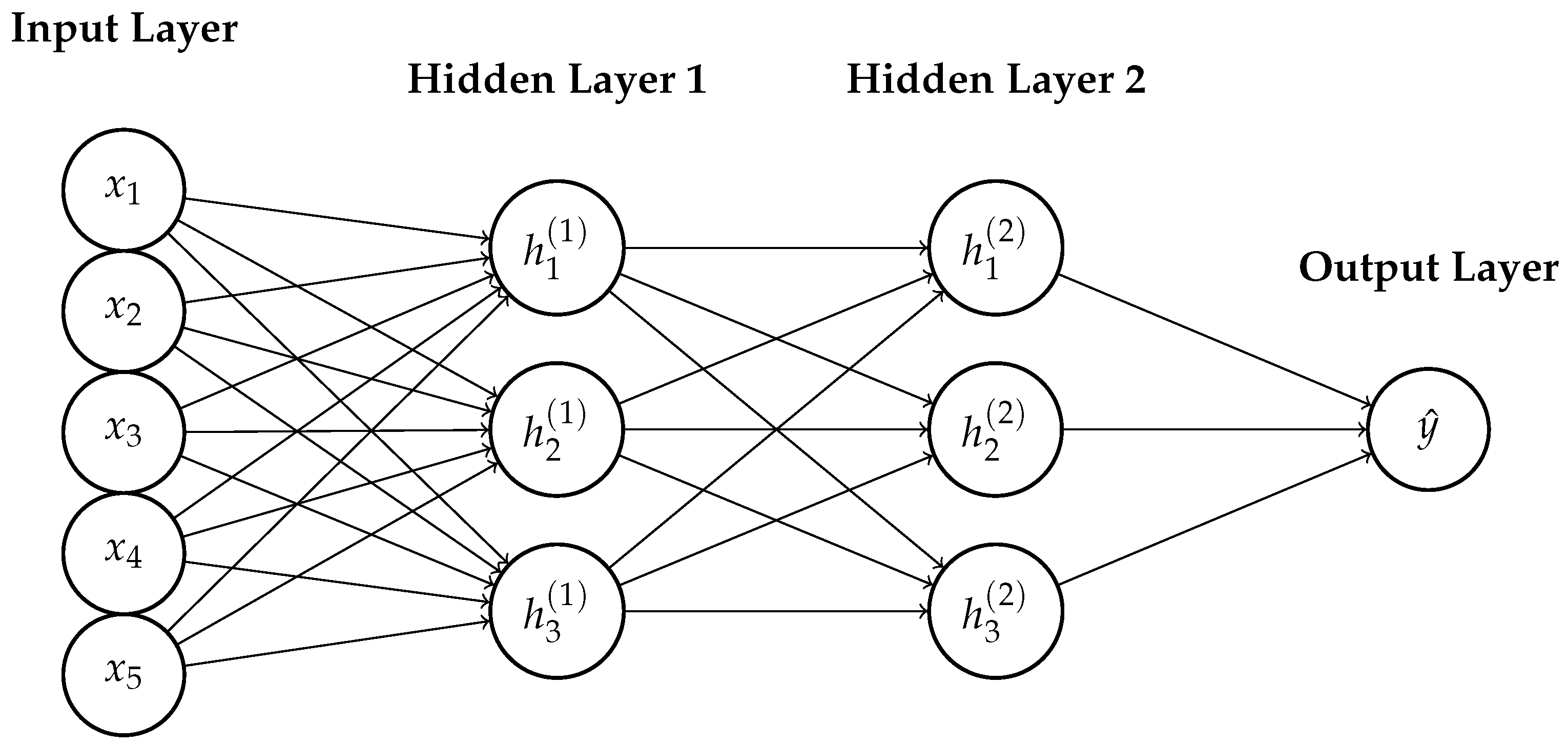
Figure A3.
A schematic diagram of the LeNet-5 architecture.
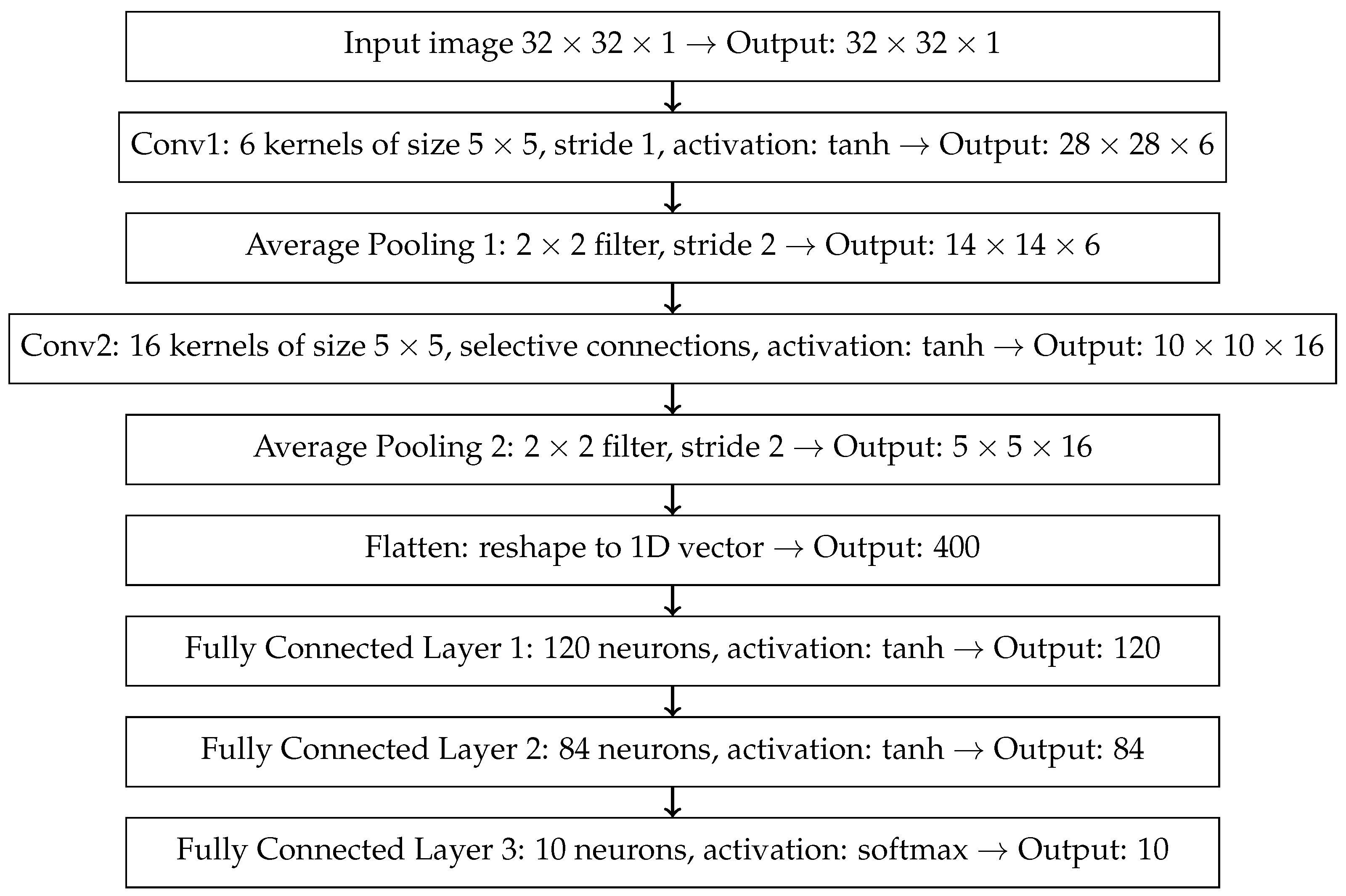
Figure A4.
A schematic diagram of the AlexNet architecture.
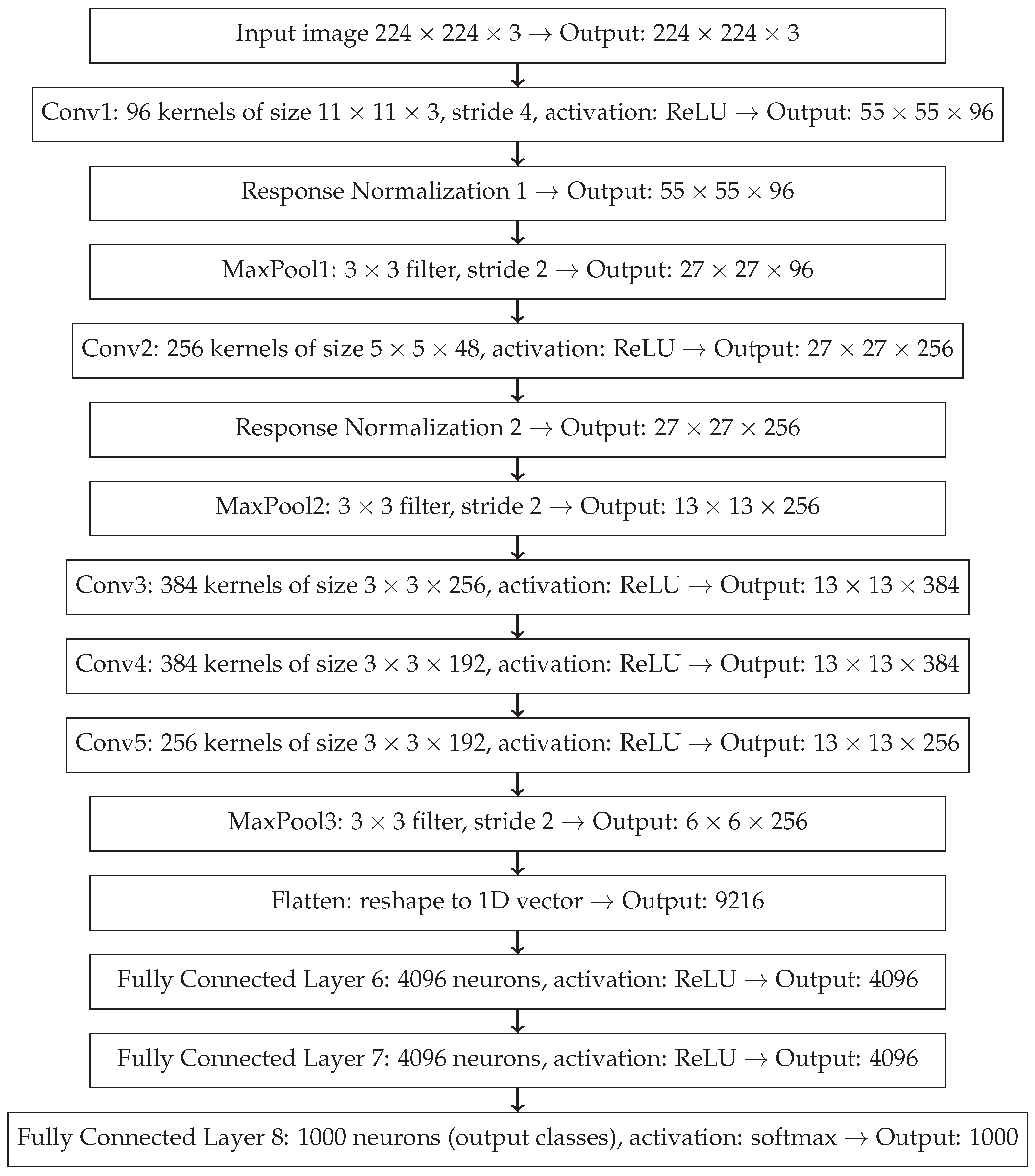
Figure A5.
A schematic diagram of the basic VGG architecture module.
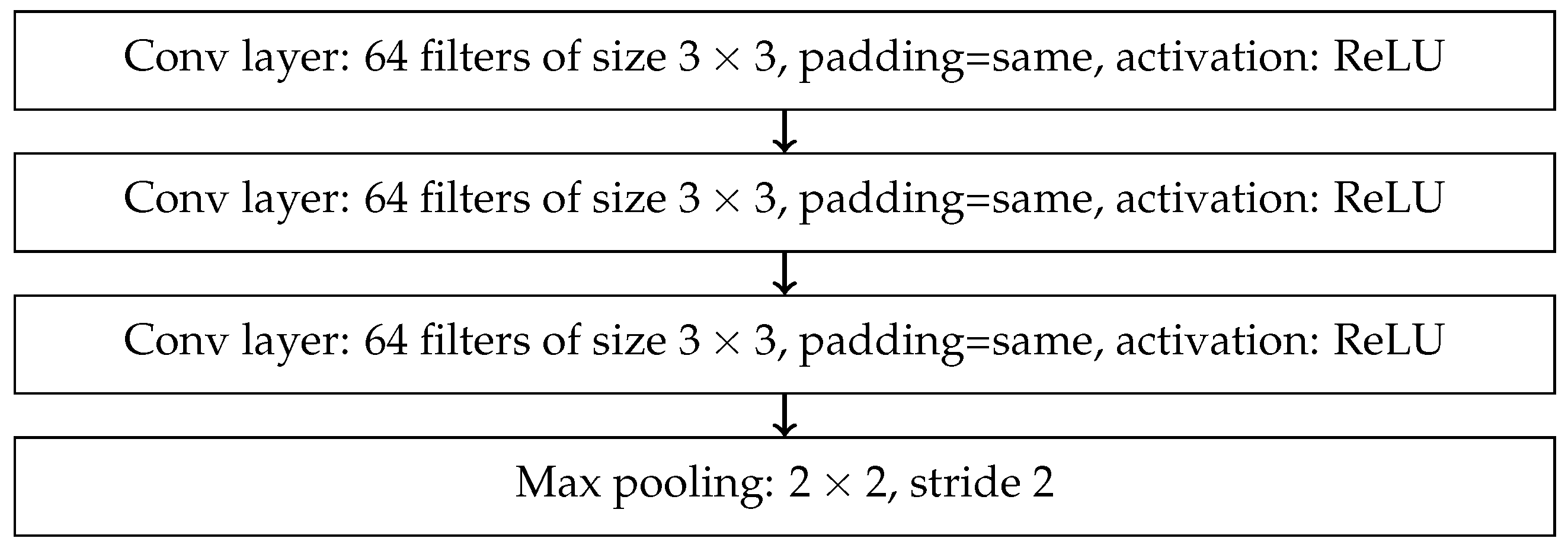
Figure A6.
A schematic diagram of the basic residual block in the ResNet architecture with skip connection.
Figure A6.
A schematic diagram of the basic residual block in the ResNet architecture with skip connection.
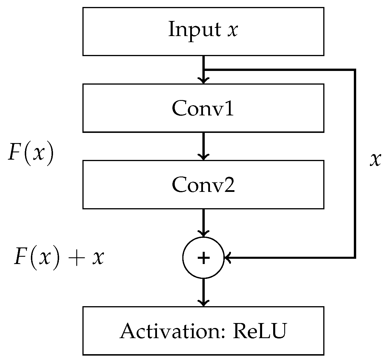
Figure A7.
A schematic diagram of the ResNeXt block: aggregated residual block with multiple parallel convolutional paths.
Figure A7.
A schematic diagram of the ResNeXt block: aggregated residual block with multiple parallel convolutional paths.
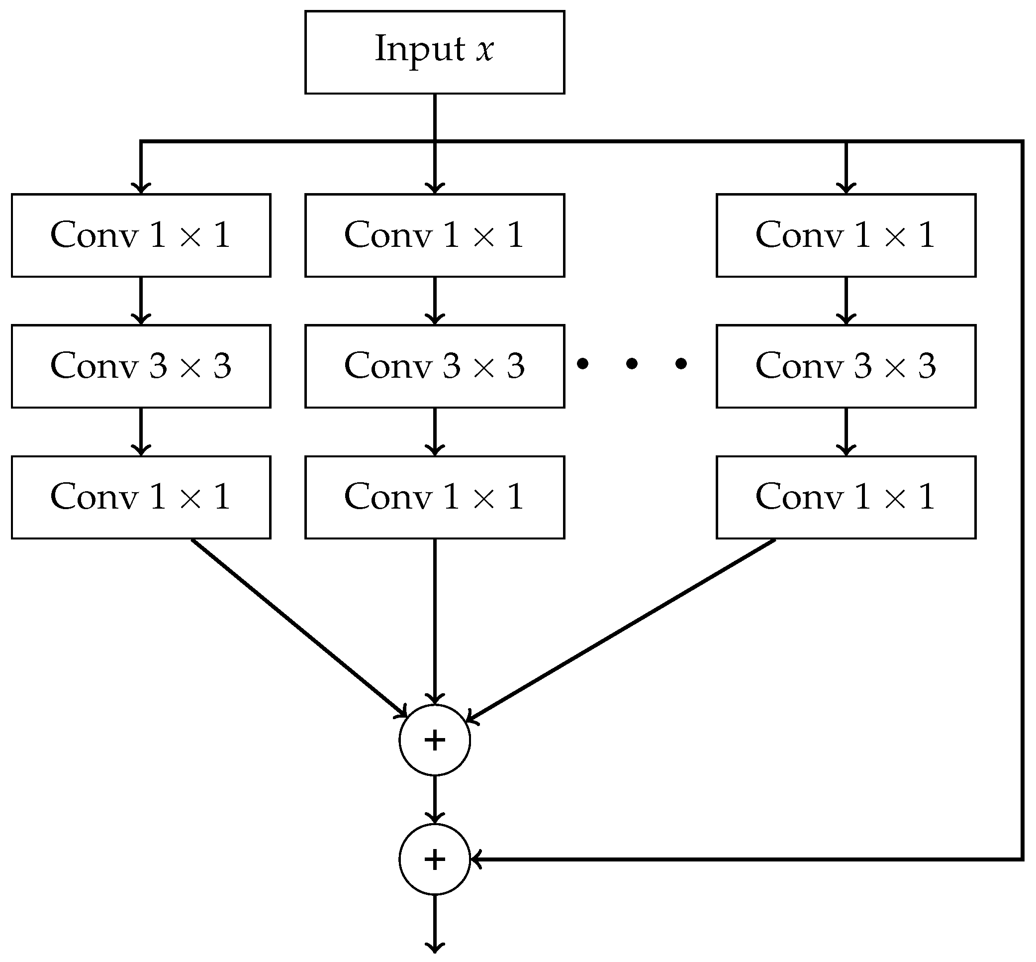
Figure A8.
A schematic diagram of the Inception module [94].
Figure A8.
A schematic diagram of the Inception module [94].
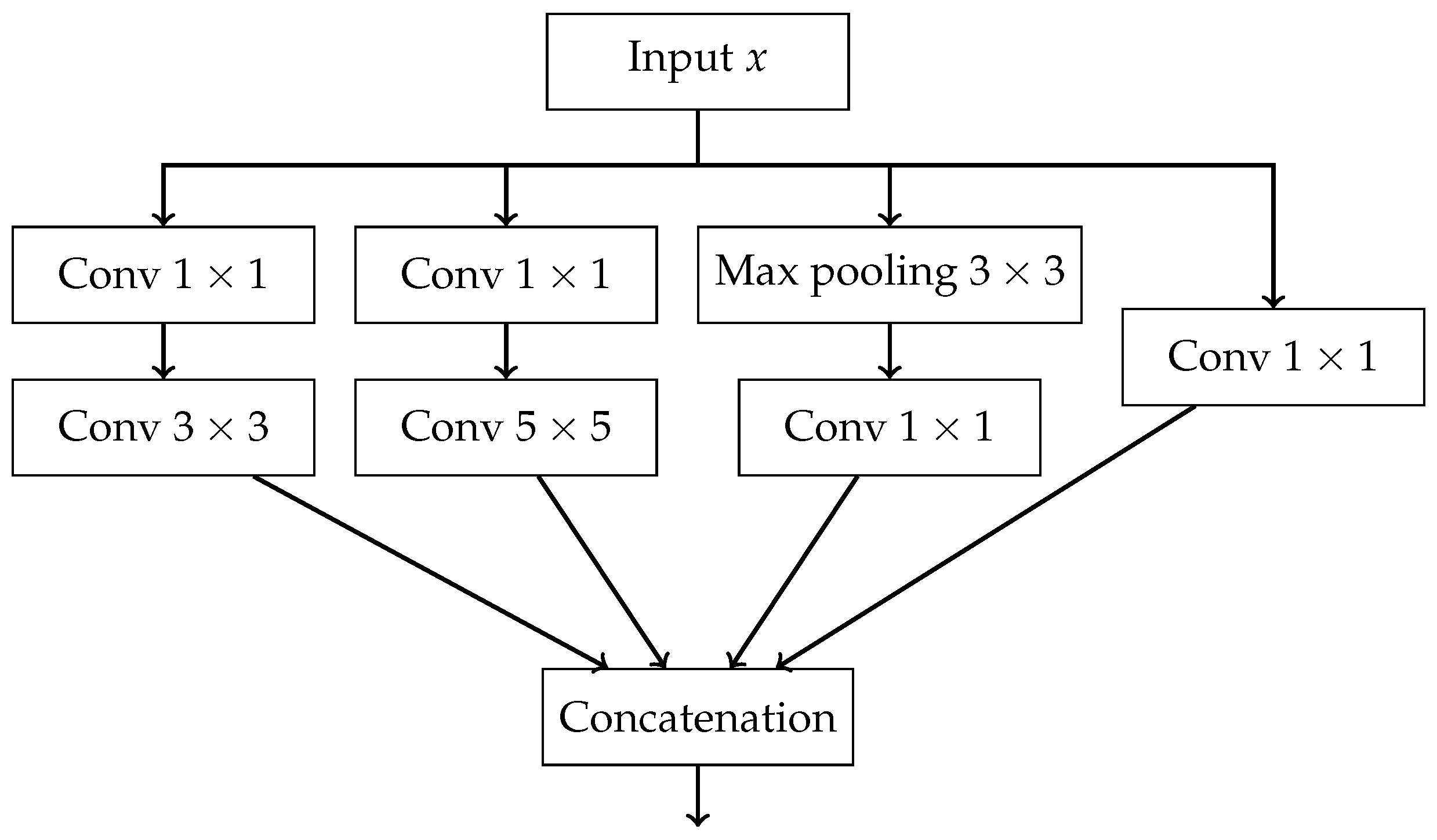
Figure A9.
A schematic diagram of the Xnception module.
References
- International Agency for Research on Cancer. Global Cancer Observatory: Cancer Today, 2024. Available from: https://gco.iarc.fr/today, Accessed: 2025-07-09.
- Medycyna Praktyczna – Podręcznik Pediatrii. Epidemiologia. Zagadnienia ogólne – Nowotwory wieku dziecięcego. https://www.mp.pl/podrecznik/pediatria/chapter/B42.71.13.1, 2025. Accessed: 2025-07-09.
- Siegel, R.L.; Giaquinto, A.N.; Jemal, A. Cancer statistics, 2024. CA: A Cancer Journal for Clinicians 2024, 74, 12–49, [https://acsjournals.onlinelibrary.wiley.com/doi/pdf/10.3322/caac.21820]. [Google Scholar] [CrossRef] [PubMed]
- Zhang, N.; Wu, J.; Wang, Q.; Liang, Y.; Li, X.; Chen, G.; Ma, L.; Liu, X.; Zhou, F. Global burden of hematologic malignancies and evolution patterns over the past 30 years. Blood Cancer Journal 2023, 13. [Google Scholar] [CrossRef]
- Ross, M.H.; Pawlina, W. Histology: A Text and Atlas. With Correlated Cell and Molecular Biology; Lippincott Williams & Wilkins: Philadelphia, 2019; p. 314. [Google Scholar]
- Tsukasaki, K. Adult T-cell leukemia-lymphoma. Hematology 2012, 17. [Google Scholar] [CrossRef]
- Arber, D.A.; Orazi, A.; Hasserjian, R.P.; Borowitz, M.J.; Calvo, K.R.; Kvasnicka, H.M.; Wang, S.A.; Bagg, A.; Barbui, T.; Branford, S.; et al. International Consensus Classification of Myeloid Neoplasms and Acute Leukemias: integrating morphologic, clinical, and genomic data. Blood 2022, 140, 1200–1228. [Google Scholar] [CrossRef]
- Mendez-Hernandez, A.; Moturi, K.; Hanson, V.; Andritsos, L.A. Hairy Cell Leukemia: Where Are We in 2023?, 2023. [CrossRef]
- Gutierrez, M.; Bladek, P.; Goksu, B.; Murga-Zamalloa, C.; Bixby, D.; Wilcox, R. T-Cell Prolymphocytic Leukemia: Diagnosis, Pathogenesis, and Treatment, 2023. [CrossRef]
- Drillet, G.; Pastoret, C.; Moignet, A.; Lamy, T.; Marchand, T. Large granular lymphocyte leukemia: An indolent clonal proliferative disease associated with an array of various immunologic disorders. La Revue de Médecine Interne 2023, 44, 295–306. [Google Scholar] [CrossRef]
- George, B.S.; Yohannan, B.; Gonzalez, A.; Rios, A. Mixed-Phenotype Acute Leukemia: Clinical Diagnosis and Therapeutic Strategies. Biomedicines 2022, 10. [Google Scholar] [CrossRef]
- Bennett, J.M.; Catovsky, D.; Daniel, M.T.; Flandrin, G.; Galton, D.A.G.; Gralnick, H.R.; Sultan, C. Proposals for the Classification of the Acute Leukaemias French-American-British (FAB) Co-operative Group. British Journal of Haematology 1976, 33, 451–458, [https://onlinelibrary.wiley.com/doi/pdf/10.1111/j.1365-2141.1976.tb03563.x]. [Google Scholar] [CrossRef]
- Meaghan, M. Ryan, MSN, F.B. Acute Promyelocytic Leukemia: A Summary. Journal of the Advanced Practitioner in Oncology 2018, 9. [Google Scholar] [CrossRef]
- Hallek, M.; Shanafelt, T.D.; Eichhorst, B. Seminar Chronic lymphocytic leukaemia. The Lancet 2018, 391, 1524–1537. [Google Scholar] [CrossRef] [PubMed]
- Epidemiological, genetic, and clinical characterization by age of newly diagnosed acute myeloid leukemia based on an academic population-based registry study (AMLSG BiO). Annals of Hematology 2017, 96, 1993–2003. [CrossRef] [PubMed]
- Puckett, Y.; Chan, O. Acute Lymphocytic Leukemia; StatPearls Publishing: Treasure Island (FL), 2023. Updated 2023 Aug 26. Available at: https://www.ncbi.nlm.nih.gov/books/NBK459149/. Accessed: 2025-07-20.
- American Cancer Society. Key Statistics for Chronic Myeloid Leukemia. https://www.cancer.org/cancer/types/chronic-myeloid-leukemia/about/statistics.html, 2025. Accessed: 2025-07-20.
- American Cancer Society. Key Statistics for Chronic Lymphocytic Leukemia. https://www.cancer.org/cancer/types/chronic-lymphocytic-leukemia/about/key-statistics.html, 2025. Accessed: 2025-07-20.
- Park, S.; Park, Y.H.; Huh, J.; Baik, S.M.; Park, D.J. Deep learning model for differentiating acute myeloid and lymphoblastic leukemia in peripheral blood cell images via myeloblast and lymphoblast classification. Digital Health 2024, 10. [Google Scholar] [CrossRef]
- Chiaretti, S.; Zini, G.; Bassan, R. Diagnosis and subclassification of acute lymphoblastic leukemia, 2014. [CrossRef]
- Eden, R.E.; Coviello, J.M. Chronic Myelogenous Leukemia; StatPearls Publishing: Treasure Island (FL), 2023. Updated 2023 Jan 16. Available from: https://www.ncbi.nlm.nih.gov/books/NBK531459/. Accessed: 2025-07-20.
- Penn Medicine. Chronic Myeloid Leukemia. https://www.pennmedicine.org/conditions/chronic-myeloid-leukemia, 2025. Accessed: 2025-07-20.
- Rai, K.R.; Sawitsky, A.; Cronkite, E.P.; Chanana, A.D.; Levy, R.N.; Pasternack, B.S. Clinical Staging of Chronic Lymphocytic Leukemia. Blood 1975, 46, 219–234. [Google Scholar] [CrossRef]
- Zengin, N.; Kars, A.; Kansu, E.; Ozdemir, O.; Barista, I.; Gullu, I.; Guler, N.; Ozisik, Y.; Dundar, S.; Firat, D. Comparison of Rai and Binet classifications in chronic lymphocytic leukemia. Hematology 1997, 2, 125–129. [Google Scholar] [CrossRef]
- WHO Classification of Tumours Editorial Board. Haematolymphoid tumours [Internet]. Lyon (France): International Agency for Research on Cancer, 2024. WHO classification of tumours series, 5th ed.; vol. 11. Available from: https://tumourclassification.iarc.who.int/chapters/63. Accessed: 2025-07-20.
- Bain, B.J. Routine and specialised techniques in the diagnosis of haematological neoplasms. Journal of Clinical Pathology 1995, 48, 501–508, [https://jcp.bmj.com/content/48/6/501.full.pdf]. [Google Scholar] [CrossRef] [PubMed]
- Dehkharghanian, T.; Mu, Y.; Tizhoosh, H.R.; Campbell, C.J. Applied machine learning in hematopathology, 2023. [CrossRef]
- Browman, G.P.; Neame, P.B.; Soamboonsrup, P. The Contribution of Cytochemistry and Immunophenotyping to the Reproducibility of the FAB Classification in Acute Leukemia. Blood 1986, 68, 900–905. [Google Scholar] [CrossRef] [PubMed]
- Eckardt, J.N.; Schmittmann, T.; Riechert, S.; Kramer, M.; Sulaiman, A.S.; Sockel, K.; Kroschinsky, F.; Schetelig, J.; Wagenführ, L.; Schuler, U.; et al. Deep learning identifies Acute Promyelocytic Leukemia in bone marrow smears. BMC Cancer 2022, 22. [Google Scholar] [CrossRef]
- Karar, M.E.; Alotaibi, B.; Alotaibi, M. Intelligent Medical IoT-Enabled Automated Microscopic Image Diagnosis of Acute Blood Cancers. Sensors 2022, 22. [Google Scholar] [CrossRef]
- Rastogi, P.; Khanna, K.; Singh, V. LeuFeatx: Deep learning–based feature extractor for the diagnosis of acute leukemia from microscopic images of peripheral blood smear. Computers in Biology and Medicine 2022, 142. [Google Scholar] [CrossRef]
- Musleh, S.; Islam, M.T.; Alam, M.T.; Househ, M.; Shah, Z.; Alam, T. ALLD: Acute Lymphoblastic Leukemia Detector. In Proceedings of the Studies in Health Technology and Informatics. IOS Press BV; 2022; Vol. 289, pp. 77–80. [Google Scholar] [CrossRef]
- Jawahar, M.; H, S.; L, J.A.; Gandomi, A.H. ALNett: A cluster layer deep convolutional neural network for acute lymphoblastic leukemia classification. Computers in Biology and Medicine 2022, 148. [Google Scholar] [CrossRef]
- Abunadi, I.; Senan, E.M. Multi-Method Diagnosis of Blood Microscopic Sample for Early Detection of Acute Lymphoblastic Leukemia Based on Deep Learning and Hybrid Techniques. Sensors 2022, 22. [Google Scholar] [CrossRef] [PubMed]
- Manescu, P.; Narayanan, P.; Bendkowski, C.; Elmi, M.; Claveau, R.; Pawar, V.; Brown, B.J.; Shaw, M.; Rao, A.; Fernandez-Reyes, D. Detection of acute promyelocytic leukemia in peripheral blood and bone marrow with annotation-free deep learning. Scientific Reports 2023, 13. [Google Scholar] [CrossRef]
- Ouyang, N.; Wang, W.; Ma, L.; Wang, Y.; Chen, Q.; Yang, S.; Xie, J.; Su, S.; Cheng, Y.; Cheng, Q.; et al. Diagnosing acute promyelocytic leukemia by using convolutional neural network. Clinica Chimica Acta 2021, 512, 1–6. [Google Scholar] [CrossRef] [PubMed]
- Osman, M.; Akkus, Z.; Jevremovic, D.; Nguyen, P.L.; Roh, D.; Al-Kali, A.; Patnaik, M.M.; Nanaa, A.; Rizk, S.; Salama, M.E. Classification of monocytes, promonocytes and monoblasts using deep neural network models: An area of unmet need in diagnostic hematopathology. Journal of Clinical Medicine 2021, 10. [Google Scholar] [CrossRef] [PubMed]
- Boldú, L.; Merino, A.; Acevedo, A.; Molina, A.; Rodellar, J. A deep learning model (ALNet) for the diagnosis of acute leukaemia lineage using peripheral blood cell images. Computer Methods and Programs in Biomedicine 2021, 202. [Google Scholar] [CrossRef] [PubMed]
- Pałczyński, K.; Śmigiel, S.; Gackowska, M.; Ledziński, D.; Bujnowski, S.; Lutowski, Z. IoT application of transfer learning in hybrid artificial intelligence systems for acute lymphoblastic leukemia classification. Sensors 2021, 21. [Google Scholar] [CrossRef]
- Jiang, Z.; Dong, Z.; Wang, L.; Jiang, W. Method for Diagnosis of Acute Lymphoblastic Leukemia Based on ViT-CNN Ensemble Model. Computational Intelligence and Neuroscience 2021, 2021. [Google Scholar] [CrossRef]
- Chen, Y.M.; Chou, F.I.; Ho, W.H.; Tsai, J.T. Classifying microscopic images as acute lymphoblastic leukemia by Resnet ensemble model and Taguchi method. BMC Bioinformatics 2021, 22. [Google Scholar] [CrossRef]
- Dese, K.; Raj, H.; Ayana, G.; Yemane, T.; Adissu, W.; Krishnamoorthy, J.; Kwa, T. Accurate Machine-Learning-Based classification of Leukemia from Blood Smear Images. Clinical Lymphoma, Myeloma and Leukemia 2021, 21, e903–e914. [Google Scholar] [CrossRef]
- Haferlach, T.; Pohlkamp, C.; Heo, I.; Drescher, R.; Hänselmann, S.; Lörch, T.; Kern, W.; Haferlach, C.; Nadarajah, N. Automated Peripheral Blood Cell Differentiation Using Artificial Intelligence - a Study with More Than 10,000 Routine Samples in a Specialized Leukemia Laboratory. Blood 2021, 138, 103–103. [Google Scholar] [CrossRef]
- Hussein, S.E.; Chen, P.; Medeiros, L.J.; Wistuba, I.I.; Jaffray, D.; Wu, J.; Khoury, J.D. Artificial intelligence strategy integrating morphologic and architectural biomarkers provides robust diagnostic accuracy for disease progression in chronic lymphocytic leukemia. Journal of Pathology 2022, 256, 4–14. [Google Scholar] [CrossRef]
- Liu, K.; Hu, J. Classification of acute myeloid leukemia M1 and M2 subtypes using machine learning. Computers in Biology and Medicine 2022, 147. [Google Scholar] [CrossRef]
- Eckardt, J.N.; Middeke, J.; Riechert, S.; Schmittmann, T.; Sulaiman, A.; Kramer, M.; Sockel, K.; Kroschinsky, P.; Schuler, U.; Schetelig, J.; et al. Deep learning detects acute myeloid leukemia and predicts NPM1 mutation status from bone marrow smears. Leukemia 2022, 36, 1–8. [Google Scholar] [CrossRef]
- Wang, W.; Luo, M.; Guo, P.; Wei, Y.; Tan, Y.; Shi, H. Artificial intelligence-assisted diagnosis of hematologic diseases based on bone marrow smears using deep neural networks. Computer Methods and Programs in Biomedicine 2023, 231. [Google Scholar] [CrossRef]
- Abhishek, A.; Jha, R.K.; Sinha, R.; Jha, K. Automated detection and classification of leukemia on a subject-independent test dataset using deep transfer learning supported by Grad-CAM visualization. Biomedical Signal Processing and Control 2023, 83. [Google Scholar] [CrossRef]
- Zhang, Z.; Arabyarmohammadi, S.; Leo, P.; Meyerson, H.; Metheny, L.; Xu, J.; Madabhushi, A. Automatic myeloblast segmentation in acute myeloid leukemia images based on adversarial feature learning. Computer Methods and Programs in Biomedicine 2024, 243. [Google Scholar] [CrossRef] [PubMed]
- Xiao, Y.; Huang, Z.; Wu, J.; Zhang, Y.; Yang, Y.; Xu, C.; Guo, F.; Ni, X.; Hu, X.; Yang, J.; et al. Rapid screening of acute promyelocytic leukaemia in daily batch specimens: A novel artificial intelligence-enabled approach to bone marrow morphology. Clinical and Translational Medicine 2024, 14. [Google Scholar] [CrossRef]
- Huang, M.L.; Huang, Z.B. An ensemble-acute lymphoblastic leukemia model for acute lymphoblastic leukemia image classification. Mathematical Biosciences and Engineering 2024, 21, 1959–1978. [Google Scholar] [CrossRef] [PubMed]
- Jawahar, M.; Anbarasi, L.J.; Narayanan, S.; Gandomi, A.H. An attention-based deep learning for acute lymphoblastic leukemia classification. Scientific Reports 2024, 14. [Google Scholar] [CrossRef]
- Aby, A.E.; Salaji, S.; Anilkumar, K.K.; Rajan, T. Classification of acute myeloid leukemia by pre-trained deep neural networks: A comparison with different activation functions. Medical Engineering and Physics 2025, 135. [Google Scholar] [CrossRef]
- Mehan, V. Artificial Intelligence Powered Automated and Early Diagnosis of Acute Lymphoblastic Leukemia Cancer in Histopathological Images: A Robust SqueezeNet-Enhanced Machine Learning Framework. International Journal of Telemedicine and Applications 2025, 2025. [Google Scholar] [CrossRef]
- Labati, R.D.; Piuri, V.; Scotti, F. All-IDB: The acute lymphoblastic leukemia image database for image processing. In Proceedings of the 2011 18th IEEE international conference on image processing. IEEE; 2011; pp. 2045–2048. [Google Scholar]
- Fišer, K.; Sieger, T.; Schumich, A.; Wood, B.; Irving, J.; Mejstříková, E.; Dworzak, M.N. Detection and monitoring of normal and leukemic cell populations with hierarchical clustering of flow cytometry data. Cytometry Part A 2012, 81A, 25–34, [https://onlinelibrary.wiley.com/doi/pdf/10.1002/cyto.a.21148]. [Google Scholar] [CrossRef]
- Agaian, S.; Madhukar, M.; Chronopoulos, A.T. Automated screening system for acute myelogenous leukemia detection in blood microscopic images. IEEE Systems Journal 2014, 8, 995–1004. [Google Scholar] [CrossRef]
- Putzu, L.; Caocci, G.; Ruberto, C.D. Leucocyte classification for leukaemia detection using image processing techniques. Artificial Intelligence in Medicine 2014, 62, 179–191. [Google Scholar] [CrossRef]
- Neoh, S.C.; Srisukkham, W.; Zhang, L.; Todryk, S.; Greystoke, B.; Lim, C.P.; Hossain, M.A.; Aslam, N. An Intelligent Decision Support System for Leukaemia Diagnosis using Microscopic Blood Images OPEN. Nature Publishing Group 2015, 5, 14938. [Google Scholar] [CrossRef]
- Rawat, J.; Singh, A.; Bhadauria, H.S.; Virmani, J. Computer Aided Diagnostic System for Detection of Leukemia Using Microscopic Images. In Proceedings of the Procedia Computer Science. Elsevier B.V. 2015; Vol. 70, pp. 748–756. [Google Scholar] [CrossRef]
- Kazemi, F.; Najafabadi, T.; Araabi, B. Automatic Recognition of Acute Myelogenous Leukemia in Blood Microscopic Images Using K-means Clustering and Support Vector Machine. Journal of medical signals and sensors 2016, 6, 183–93. [Google Scholar] [CrossRef] [PubMed]
- Bigorra, L.; Merino, A.; Alférez, S.; Rodellar, J. Feature Analysis and Automatic Identification of Leukemic Lineage Blast Cells and Reactive Lymphoid Cells from Peripheral Blood Cell Images. Journal of Clinical Laboratory Analysis 2017, 31. [Google Scholar] [CrossRef]
- Rawat, J.; Singh, A.; Bhadauria, H.S.; Virmani, J.; Devgun, J.S. Classification of acute lymphoblastic leukaemia using hybrid hierarchical classifiers. Multimedia Tools and Applications 2017, 76, 19057–19085. [Google Scholar] [CrossRef]
- Mooney, P.T. Blood Cells. Kaggle dataset, 2025. Downloaded from https://www.kaggle.com/datasets/paultimothymooney/blood-cells.
- Rehman, A.; Abbas, N.; Saba, T.; Rahman, S.I.u.; Mehmood, Z.; Kolivand, H. Classification of acute lymphoblastic leukemia using deep learning. Microscopy Research and Technique 2018, 81, 1310–1317, [https://analyticalsciencejournals.onlinelibrary.wiley.com/doi/pdf/10.1002/jemt.23139]. [Google Scholar] [CrossRef]
- Shafique, S.; Tehsin, S. Acute lymphoblastic leukemia detection and classification of its subtypes using pretrained deep convolutional neural networks. Technology in Cancer Research and Treatment 2018, 17, 1–7. [Google Scholar] [CrossRef] [PubMed]
- Khosla, E.; Ramesh, D. Phase classification of chronic myeloid leukemia using convolution neural networks. In Proceedings of the Proceedings of the 4th IEEE International Conference on Recent Advances in Information Technology, RAIT 2018. Institute of Electrical and Electronics Engineers Inc., 6 2018, pp. 1–6. [CrossRef]
- Huang, F.; Guang, P.; Li, F.; Liu, X.; Zhang, W.; Huang, W.; Haque, N. AML, ALL, and CML classification and diagnosis based on bone marrow cell morphology combined with convolutional neural network: A STARD compliant diagnosis research. Medicine (United States) 2020, 99, E23154. [Google Scholar] [CrossRef] [PubMed]
- Chandradevan, R.; Aljudi, A.A.; Drumheller, B.R.; Kunananthaseelan, N.; Amgad, M.; Gutman, D.A.; Cooper, L.A.; Jaye, D.L. Machine-based detection and classification for bone marrow aspirate differential counts: initial development focusing on nonneoplastic cells. Laboratory Investigation 2020, 100, 98–109. [Google Scholar] [CrossRef]
- Rösler, W.; Altenbuchinger, M.; Baeßler, B.; Beissbarth, T.; Beutel, G.; Bock, R.; von Bubnoff, N.; Eckardt, J.N.; Foersch, S.; Loeffler, C.M.; et al. An overview and a roadmap for artificial intelligence in hematology and oncology. Journal of Cancer Research and Clinical Oncology 2023, 149, 7997. [Google Scholar] [CrossRef]
- Kowalski, P.; Smyk, R. Comparison of thresholding algorithms for automatic overhead line detection procedure. Przegląd Elektrotechniczny 2022, pp. 149–155.
- Hough, P.V. Method and means for recognizing complex patterns, 1962. US Patent 3,069,654.
- Duda, R.O.; Hart, P.E. Use of the Hough transformation to detect lines and curves in pictures. Communications of the ACM 1972, 15, 11–15. [Google Scholar] [CrossRef]
- Ballard, D.H. Generalizing the Hough transform to detect arbitrary shapes. Pattern recognition 1981, 13, 111–122. [Google Scholar] [CrossRef]
- Shalev-Shwartz, S.; Ben-David, S. Understanding machine learning: From theory to algorithms; Cambridge University Press, 2014.
- Breiman, L. Random forests. Machine learning 2001, 45, 5–32. [Google Scholar] [CrossRef]
- Friedman, J.H. Greedy function approximation: a gradient boosting machine. Annals of statistics 2001, pp. 1189–1232.
- Cox, D.R. The regression analysis of binary sequences. Journal of the Royal Statistical Society Series B: Statistical Methodology 1958, 20, 215–232. [Google Scholar] [CrossRef]
- Ruder, S. An overview of gradient descent optimization algorithms. arXiv preprint 2016, arXiv:1609.04747 2016. [Google Scholar]
- Tibshirani, R. Regression shrinkage and selection via the lasso. Journal of the Royal Statistical Society Series B: Statistical Methodology 1996, 58, 267–288. [Google Scholar] [CrossRef]
- Hoerl, A.E.; Kennard, R.W. Ridge regression: Biased estimation for nonorthogonal problems. Technometrics 1970, 12, 55–67. [Google Scholar] [CrossRef]
- Zou, H.; Hastie, T. Regularization and variable selection via the elastic net. Journal of the Royal Statistical Society Series B: Statistical Methodology 2005, 67, 301–320, [https://academic.oup.com/jrsssb/articlepdf/2967/2/301/49795094/jrsssb_67_2_301.pdf]. [Google Scholar] [CrossRef]
- Cortes, C.; Vapnik, V. Support-vector networks. Machine learning 1995, 20, 273–297. [Google Scholar] [CrossRef]
- Lloyd, S. Least squares quantization in PCM. IEEE transactions on information theory 1982, 28, 129–137. [Google Scholar] [CrossRef]
- LeCun, Y.; Bottou, L.; Bengio, Y.; Haffner, P. Gradient-based learning applied to document recognition. Proceedings of the IEEE 1998, 86, 2278–2324. [Google Scholar] [CrossRef]
- Roberts, L. Machine Perception of Three-Dimensional Solids. PhD thesis, 1963.
- Sobel, I.; Feldman, G. A 3×3 isotropic gradient operator for image processing. Pattern Classification and Scene Analysis 1973, pp. 271–272.
- Prewitt, J.M.; et al. Object enhancement and extraction. Picture processing and Psychopictorics 1970, 10, 15–19. [Google Scholar]
- Krizhevsky, A.; Sutskever, I.; Hinton, G.E. Imagenet classification with deep convolutional neural networks. Advances in neural information processing systems 2012, 25. [Google Scholar] [CrossRef]
- Simonyan, K.; Zisserman, A. Very deep convolutional networks for large-scale image recognition. arXiv preprint 2014, arXiv:1409.1556 2014. [Google Scholar]
- He, K.; Zhang, X.; Ren, S.; Sun, J. Deep residual learning for image recognition. In Proceedings of the Proceedings of the IEEE conference on computer vision and pattern recognition, 2016, pp. 770–778.
- Xie, S.; Girshick, R.; Dollár, P.; Tu, Z.; He, K. Aggregated residual transformations for deep neural networks. In Proceedings of the Proceedings of the IEEE conference on computer vision and pattern recognition, 2017, pp. 1492–1500.
- Huang, G.; Liu, Z.; Van Der Maaten, L.; Weinberger, K.Q. Densely connected convolutional networks. In Proceedings of the Proceedings of the IEEE conference on computer vision and pattern recognition, 2017, pp. 4700–4708.
- Szegedy, C.; Liu, W.; Jia, Y.; Sermanet, P.; Reed, S.; Anguelov, D.; Erhan, D.; Vanhoucke, V.; Rabinovich, A. Going deeper with convolutions. In Proceedings of the Proceedings of the IEEE conference on computer vision and pattern recognition, 2015, pp. 1–9.
- Chollet, F. Xception: Deep learning with depthwise separable convolutions. In Proceedings of the Proceedings of the IEEE conference on computer vision and pattern recognition, 2017, pp. 1251–1258.
- Kazemi, et al.: Automatic recognition of AML in microscopic images. Technical report.
- Musleh, S.; Islam, M.T.; Alam, M.T.; Househ, M.; Shah, Z.; Alam, T. ALLD: Acute Lymphoblastic Leukemia Detector. In Proceedings of the Studies in Health Technology and Informatics. IOS Press BV; 2022; Vol. 289, pp. 77–80. [Google Scholar] [CrossRef]
- Park, S.; Park, Y.H.; Huh, J.; Baik, S.M.; Park, D.J. Deep learning model for differentiating acute myeloid and lymphoblastic leukemia in peripheral blood cell images via myeloblast and lymphoblast classification. Digital Health 2024, 10. [Google Scholar] [CrossRef]
- Xiao, Y.; Huang, Z.; Wu, J.; Zhang, Y.; Yang, Y.; Xu, C.; Guo, F.; Ni, X.; Hu, X.; Yang, J.; et al. Rapid screening of acute promyelocytic leukaemia in daily batch specimens: A novel artificial intelligence-enabled approach to bone marrow morphology. Clinical and Translational Medicine 2024, 14. [Google Scholar] [CrossRef]
- Boldú, L.; Merino, A.; Alférez, S.; Molina, A.; Acevedo, A.; Rodellar, J. Automatic recognition of different types of acute leukaemia in peripheral blood by Image Analysis. Journal of Clinical Pathology 2019, 72, 755–761. [Google Scholar] [CrossRef]
- Salah, H.T.; Muhsen, I.N.; Salama, M.E.; Owaidah, T.; Hashmi, S.K. Machine learning applications in the diagnosis of leukemia: Current trends and future directions, 2019. [CrossRef]
- Mantri, R.; Khan, R.A.H.; Mane, D.T. An Efficient System for Detection and Classification of Acute Lymphoblastic Leukemia Using Semi-Supervised Segmentation Technique. International Research Journal of Multidisciplinary Technovation 2025, 7, 121–134. [Google Scholar] [CrossRef]
- Reta, C.; Altamirano, L.; Gonzalez, J.A.; Diaz-Hernandez, R.; Peregrina, H.; Olmos, I.; Alonso, J.E.; Lobato, R. Segmentation and classification of bone marrow cells images using contextual information for medical diagnosis of acute leukemias. PloS one 2015, 10, e0130805. [Google Scholar]
- Matek, C.; Schwarz, S.; Spiekermann, K.; Marr, C. Human-level recognition of blast cells in acute myeloid leukaemia with Convolutional Neural Networks. Nature Machine Intelligence 2019, 1, 538–544. [Google Scholar] [CrossRef]
- Bhattacharjee, R.; Saini, L.M. Robust technique for the detection of Acute Lymphoblastic Leukemia. In Proceedings of the 2015 IEEE Power, Communication and Information Technology Conference (PCITC), 2015, pp. 657–662. [CrossRef]
- Rolls, G. An Introduction to Specimen Processing. https://www.leicabiosystems.com/knowledge-pathway/an-introduction-to-specimen-processing/, 2019. Accessed: 2025-07-22.
- Taqi, S.A.; Sami, S.A.; Sami, L.B.; Zaki, S.A. A review of artifacts in histopathology, 2018. [CrossRef]
- Patel, A.; Balis, U.G.; Cheng, J.; Li, Z.; Lujan, G.; Mcclintock, D.S.; Pantanowitz, L.; Parwani, A. Contemporary whole slide imaging devices and their applications within the modern pathology department: A selected hardware review, 2021. [CrossRef]
- Basak, K.; Ozyoruk, K.B.; Demir, D. Whole Slide Images in Artificial Intelligence Applications in Digital Pathology: Challenges and Pitfalls, 2023. [CrossRef]
- Sellaro, T.L.; Filkins, R.; Hoffman, C.; Fine, J.L.; Ho, J.; Parwani, A.V.; Pantanowitz, L.; Montalto, M. Relationship between magnification and resolution in digital pathology systems. Journal of Pathology Informatics 2013, 4, 21. [Google Scholar] [CrossRef] [PubMed]
- Nordin, N.; Rahim, S.N.A.; Omar, W.F.A.W.; Zulkarnain, S.; Sinha, S.; Kumar, S.; Haque, M. Preanalytical Errors in Clinical Laboratory Testing at a Glance: Source and Control Measures. Cureus 2024. [Google Scholar] [CrossRef] [PubMed]
- Nakhleh, R.E.; Idowu, M.O.; Souers, R.J.; Meier, F.A.; Leonas, G.B. Mislabeling of Cases, Specimens, Blocks, and Slides A College of American Pathologists Study of 136 Institutions. (Arch Pathol Lab Med. 2011;135:969-974) 2011.
- Packer, M.D.C.; Ravinsky, E.; Azordegan, N. Patterns of Error in Interpretive Pathology: A Review of 23 PowerPoint Presentations of Discordances. American Journal of Clinical Pathology 2021, 157, 767–773, [https://academic.oup.com/ajcp/article-pdf/157/5/767/49102733/aqab190.pdf]. [Google Scholar] [CrossRef]
- Dehan, L.M.; Lewis, J.S.; Mehrad, M.; Ely, K.A. Patterns of Major Frozen Section Interpretation Error: An In-Depth Analysis From a Complex Academic Surgical Pathology Practice. American Journal of Clinical Pathology 2023, 160, 247–254. [Google Scholar] [CrossRef] [PubMed]
- Ministerstwo Zdrowia Rzeczypospolitej Polskiej. Rozporządzenie Ministra Zdrowia z dnia 18 grudnia 2017 r. w sprawie standardów organizacyjnych opieki zdrowotnej w dziedzinie patomorfologii. Dziennik Ustaw Rzeczypospolitej Polskiej, poz. 2435/2017, Dz.U. 2017 poz. 2435, 2017. Available at: https://isap.sejm.gov.pl/isap.nsf/DocDetails.xsp?id=WDU20170002435. Accessed: 2025-07-22.
- Mutter, G.L.; Milstone, D.S.; Hwang, D.H.; Siegmund, S.; Bruce, A. Measuring digital pathology throughput and tissue dropouts. Journal of Pathology Informatics 2022, 13, 8. [Google Scholar] [CrossRef]
- Rao, G.G.; Crook, M. Pathology tests: is the time for demand management ripe at last? Technical report, 2003.
- Feng, C.; Liu, F. Artificial intelligence in renal pathology: Current status and future, 2023. [CrossRef]
- Neto, P.C.; Montezuma, D.; Oliveira, S.P.; Oliveira, D.; Fraga, J.; Monteiro, A.; Monteiro, J.; Ribeiro, L.; Gonçalves, S.; Reinhard, S.; et al. An interpretable machine learning system for colorectal cancer diagnosis from pathology slides. npj Precision Oncology 2024, 8. [Google Scholar] [CrossRef] [PubMed]
- da Silva, L.M.; Pereira, E.M.; Salles, P.G.; Godrich, R.; Ceballos, R.; Kunz, J.D.; Casson, A.; Viret, J.; Chandarlapaty, S.; Ferreira, C.G.; et al. Independent real-world application of a clinical-grade automated prostate cancer detection system. Journal of Pathology 2021, 254, 147–158. [Google Scholar] [CrossRef]
- Food and Drug Administration. Artificial Intelligence and Machine Learning (AI/ML)-Enabled Medical Devices. https://www.fda.gov/medical-devices/software-medical-device-samd/artificial-intelligence-and-machine-learning-aiml-enabled-medical-devices, 2024. Accessed: 2025-07-20.
Figure 1.
Number of publications and total citations per year over the analyzed period.
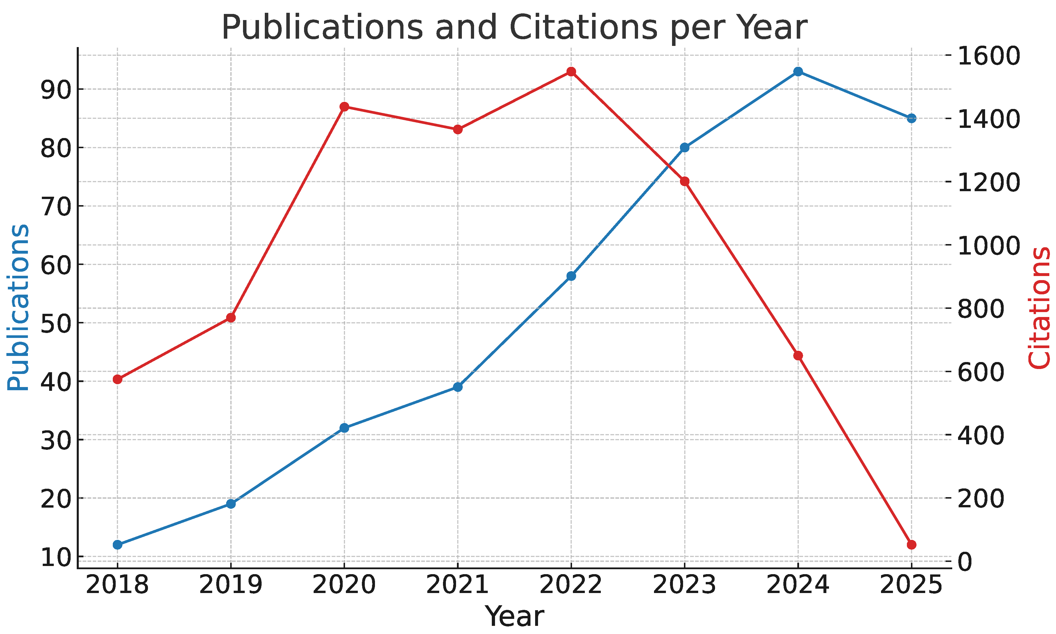
Figure 2.
Percentage share of publications by the top four contributing countries and others.
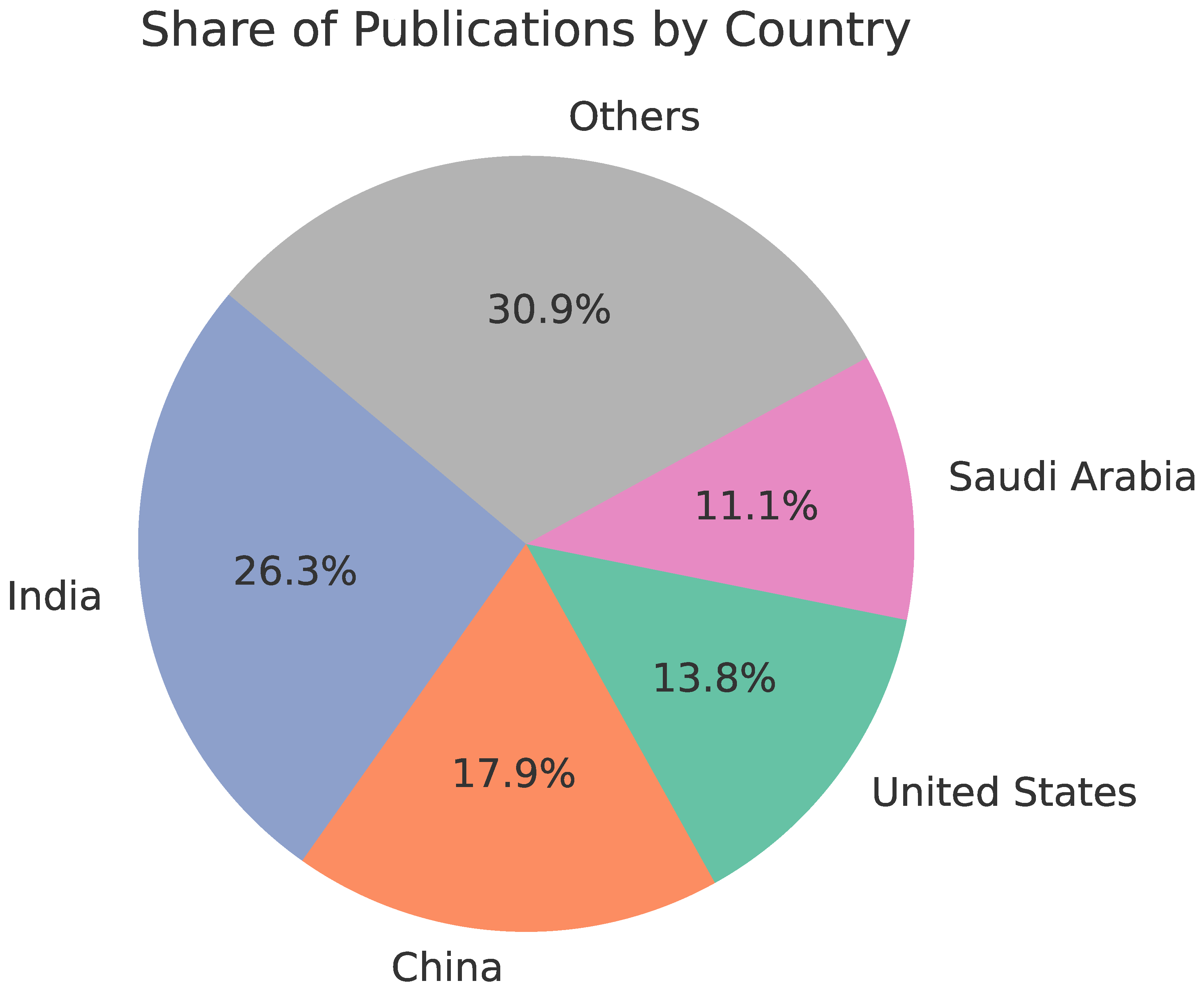
Figure 3.
Number of publications by the most active research institutions.
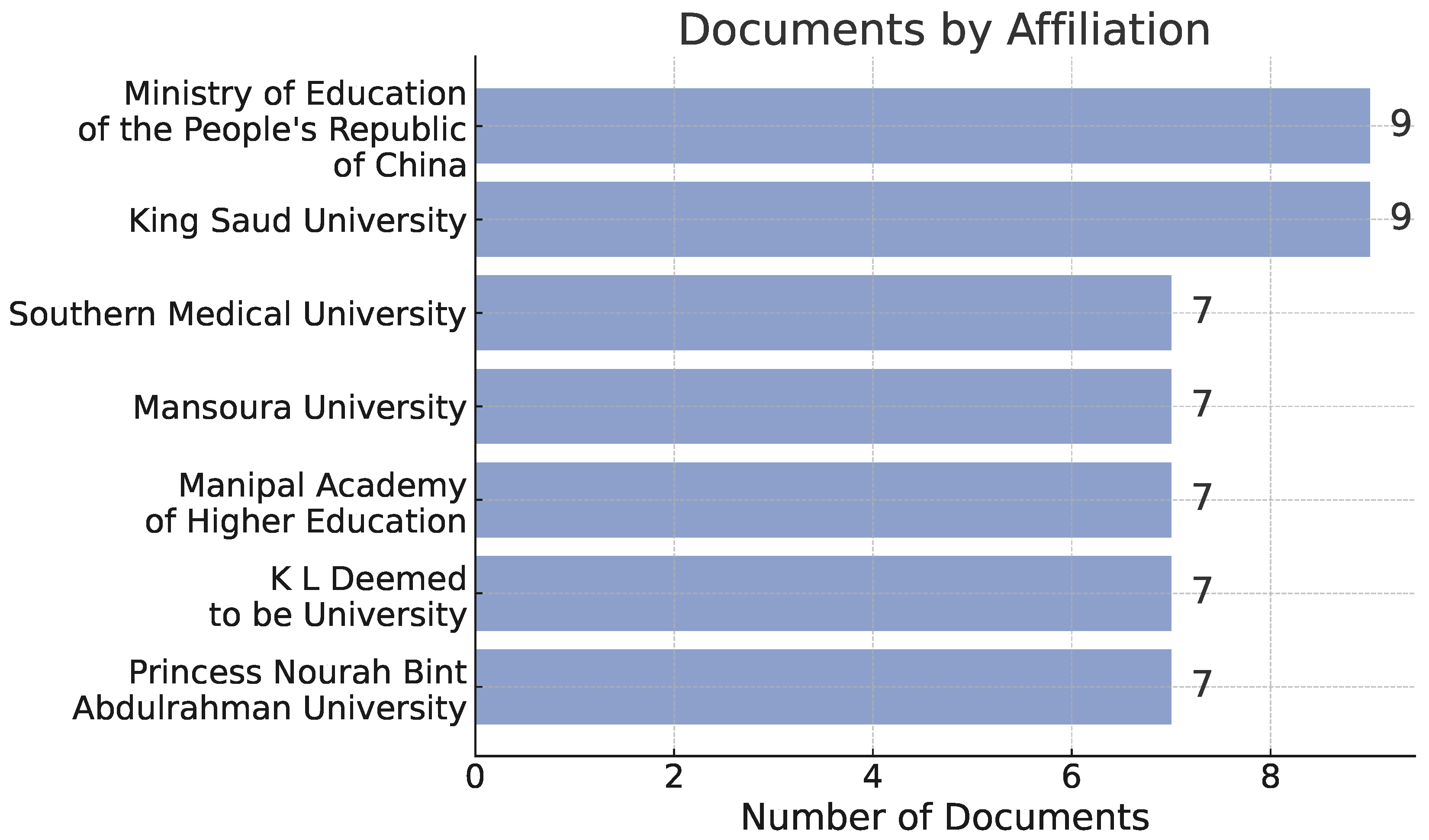
Figure 4.
Frequency of the most common keywords found in the analyzed publications.
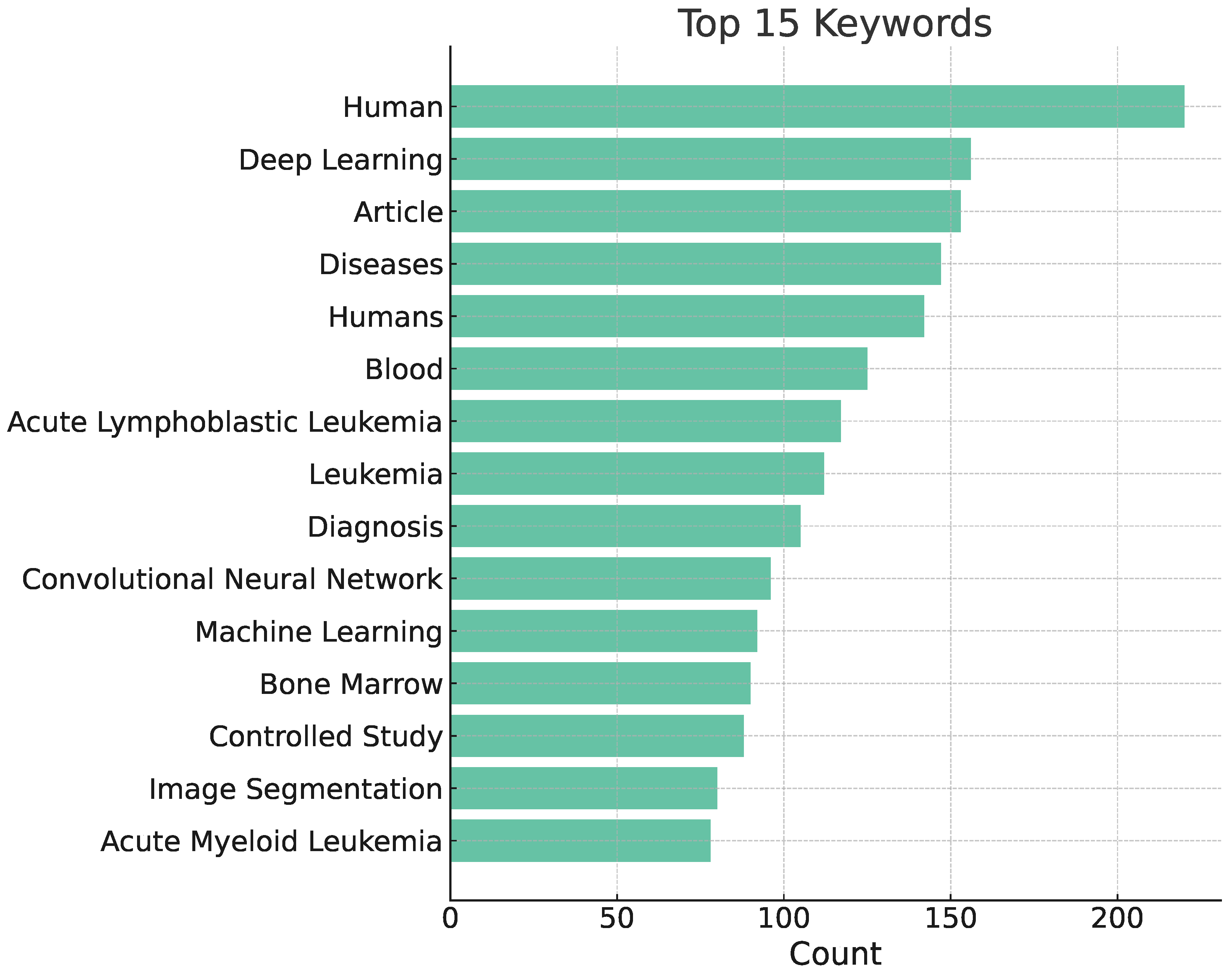

Table 1.
Overview of basic leukemia types*.
| AML | ALL | CML | CLL | |
|---|---|---|---|---|
| Median age of patient | 65 years [15] | 11 years [16] | 66 years [17] | 70 years [18] |
| Onset and disease dynamics | acute | acute | gradual | gradual |
| Subtypes, | M0-M7 (FAB) | B-ALL, T-ALL | numerous (based on genetic abnormalities) | indolent/aggressive |
| Percentage of blasts in pathological specimen required for diagnosis | 10% or 20% depending on mutations [19] | 20% lymphoblasts [20] | less than 10% in chronic phase, more than 20% in blastic phase [21] | criterion not defined for CLL |
| Staging scales | - | - | chronic, accelerated, blastic phases [22] | RAI [23], Binet [24] |
* More data on specific variants, genetic abnormalities and diagnostic criteria of leukemias and other haematological disorders can be found here: [25].
Table 2.
An overview of datasets used to train leukemia-recognition models.
| Dataset name | Year | Images | Resolution | Magnification | Problem / Type | Citations | Material |
|---|---|---|---|---|---|---|---|
| [29] | 2022 | 6 963 | X | 50 | classification | 55 | bone marrow smear |
| [30] | 2022 | 445 | X | X | classification | 47 | blood smear |
| [31] | 2022 | 18 365 | X | X | classification | 113 | blood smear |
| [32] | 2022 | 260 | X | classification | 6 | X | |
| [33] | 2022 | 10 661 | X | X | classification | 43 | X |
| [34] | 2022 | 368 | X | classification | 77 | X | |
| [35] | 2023 | 1 625 full micrographs and 20 004 single cell | 100 and 50 | classification | 40 | peripheral blood and bone marrow | |
| [36] | 2021 | 13 504 | X | X | classification | 40 | bone marrow smear |
| [37] | 2021 | 935 | 100 | classification | 13 | peripheral blood | |
| [38] | 2021 | 16 450 | X | X | classification | 140 | peripheral blood |
| [39] | 2021 | 260 | X | X | classification | 25 | blood smear |
| [40] | 2021 | 10 661 | X | X | classification | 129 | X |
| [41] | 2021 | 12 528 | X | X | classification | 23 | X |
| [42] | 2021 | 520 | 100 | classification | 90 | blood smear | |
| [43] | 2021 | 8 425 | 10 | classification | 8 | blood smear | |
| [44] | 2022 | 125 | X | 20 | classification | 41 | lymph node biopsy |
| [45] | 2022 | 122 | X | classification | 36 | bone marrow smear | |
| [46] | 2022 | 10 632 | X | 50 | classification | 86 | bone marrow smear |
| [47] | 2023 | 11 788 full micrographs and 131 300 single cell | X | X | classification | 29 | bone marrow smear |
| [48] | 2023 | 1 250 | 40 and 100 | classification | 60 | blood smear | |
| [19] | 2024 | 42 386 single cell | X | classification | 4 | peripheral blood | |
| [49] | 2024 | 204 | X | X | segmentation | 8 | cytology |
| [50] | 2024 | 15 719 | X | 10 and 100 | classification | 2 | bone marrow smear |
| [51] | 2024 | 3 527 | X | X | classification | 7 | X |
| [52] | 2024 | 362 | X | classification | 27 | X | |
| [53] | 2025 | 669 single cell | X | X | classification | 4 | X |
| [54] | 2025 | 3 256 | X | classification | X | blood smear | |
| [55] | 2011 | 109 | 300 to 500 | segmentation | 641 | blood smear | |
| [55] | 2011 | 260 | 300 to 500 | classification | 641 | blood smear | |
| [56] | 2011 | 123 | X | X | classification | 57 | bone marrow or peripheral blood |
| [57] | 2014 | 80 | X | classification | 193 | X | |
| [58] | 2014 | 33 | and | 300 to 500 | classification | 369 | X |
| [59] | 2015 | 180 | X | X | classification | 172 | blood smear |
| [60] | 2015 | 130 | X | classification | 150 | X | |
| [61] | 2016 | 330 | 100 | classification | 83 | X | |
| [62] | 2017 | 916 | X | X | classification | 50 | peripheral blood |
| [63] | 2017 | 260 | X | X | classification | 130 | X |
| [64] | 2018 | 410 | X | classification | X | blood smear | |
| [65] | 2018 | 330 | X | 100 | classification | 359 | X |
| [66] | 2018 | 368 | X | classification | 377 | X | |
| [67] | 2018 | 536 | X | classification | 10 | X | |
| [68] | 2020 | 104 | 100 | classification | 52 | bone marrow smear | |
| [69] | 2020 | 17 | X | 40 | classification | 111 | bone marrow aspirate |
Table 3.
Overview of existing AI models in leukemia diagnostics.
| Reference | Material | Diagnose | Use of the model | Dataset size | Segmentation method | Classifier | Results |
|---|---|---|---|---|---|---|---|
| [96] | blood smear, bone marrow | AML | detection of AML | 330 | pattern recognition-based | SVM | 96% accuracy |
| [62] | blood smear | AML | telling reactive lymphoid cells from myeloid and lymphoid blasts | 696 | pattern recognition-based | SVM | 82% accuracy |
| [57] | blood smear | AML | AML detection + classification into subtypes | 80 (40 ALM and 40 non-ALM) | k-means (k=3) | SVM | 98% accuracy |
| [97] | blood smear | ALL, AML | classification | 15,000 images (80/20 split, 10-fold CV for ML) | None; image resizing | DenseNet121 (DL); SVM, KNN, RF, DT (ML) | DenseNet121 → Acc: 98.7%, Prec: 98.9%, Rec: 98.3%, F1: 98.6%; SVM → Acc: 96.2% |
| [53] | blood smear | ALL, AML | classification of leukemia types | ALL-IDB (260) + LISC (257) | HSV color space + k-means clustering | Hybrid CNN + Vision Transformer (HCVT) | ALL-IDB: 99.12%, accuracy LISC: 97.28% accuracy |
| [98] | blood smear | AML, ALL | classification of AML vs ALL | 15,684 images (104 AML, 86 ALL patients) | no segmentation (weakly supervised learning on full smear images) | EfficientNet-B4 (transfer learning) | AUC = 0.981, accuracy = 95.3% |
| [99] | bone marrow smear | AML, ALL | detection | 15,719 images from 83 APL patients + 118 control samples | Color-based segmentation of karyocytes | CNN with attention modules (CELLSEE); backbones: ResNet18, ResNet34, ResNet50 | AUC = 0.9708 (CELLSEE50); Accuracy = 93.8%; Recall = 90.8% |
| [100] | blood smear | AML, ALL | X | 4394 | X | Naive Bayes, K-NN, RF, SVM | 85,8% accuracy |
| [48] | bone marrow | ALL/AML | classification into 21 morphological categories | 17152 | manual segmentation | CNN (ResNeXt) | 91.7% accuracy, avg F1-score 87.3% |
| [43] | blood smear | AML, CLL, MDS, CML, etc. | differential cell classification | 10,082 patients / 4.9M images (training: 8,425) | automatic cell cropping using scanning system | Xception | 96% accuracy; 91% blast detection; 95% concordance for pathogenic cases |
| [101] | blood smear, bone marrow | ALL, AML, CML, CLL | leukemia diagnosis | X | various (thresholding, morphological ops, clustering) | SVM, k-NN, ANN, CNN, DT, Naive Bayes, RF | accuracy ranges from 85% to >99% depending on study |
| [69] | bone marrow | AML, MM (tested), nonneoplastic (trained) | detection and classification tasks, using a two-stage system | 10,000 annotated cells (9269 nonneoplastic, plus AML, MM cases) | Faster R-CNN–based detection | VGG16 convolutional network | 97% accuracy AML |
| [102] | blood smear | ALL | segmentation and classification of blast cells | ALL-IDB: 559 | k-means | custom CNN (8 layers) | accuracy: 100% ALL detection; 99% subtypes classification |
| [54] | peripheral blood smear | Acute leukemia, MDS, CML | Automated blast detection | 114 patient samples; 100 leukocytes per smear | automated image capture and classification; no manual segmentation | CellaVision DM96 (proprietary pattern recognition system) | Sens: 93.3%, Spec: 86.8%, PPV: 87.9%, NPV: 92.6%, Acc: 90.4% |
| [103] | bone marrow | ALL | diagnosis of ALL, classification of ALL into subtypes | 633 | Pattern-recognition based | KNN, RF, SL, SVM, RC | 94% accuracy, 92% AML vs ALL |
| [37] | blood smear | ALL | classification of full smear image | 520 images; 80/20 train/test split | None; resized and normalized full images | Custom CNN (4 conv layers + dense layers) | Acc: 96.37%, Prec: 96.00%, Rec: 97.00%, F1: 96.48% |
| [49] | blood smear | ALL | classification | 392 cells (236 ALL, 156 normal), 108 images; 70/10/20 split | Manual cropping of WBC patches (224×224); no segmentation network | Vision Transformer (ViT); ViT-FF variant | Acc: 98.72%, Prec: 98.81%, Rec: 98.73%, F1: 98.72% |
| [40] | blood smear | ALL | classification | 20,000 images | Pre-segmented single-cell images; DERS augmentation | ViT + EfficientNet-b0 (ensemble, weighted sum 0.7/0.3) | Accuracy: 99.03%, Precision: 99.14% |
| [41] | blood smear | ALL | localization + classification | 392 cells (236 blast, 156 normal), 108 images | UNet (integrated in end-to-end model) | UNet + ResNet18 (ALL-NET architecture) | Acc: 98.68%, Prec: 98.70%, Rec: 98.80%, F1: 98.75% |
| [51] | blood smear | ALL | classification of leukemic vs normal cells | 260 cell images | manual cropping | custom CNN + k-NN, SVM, RF | up to 99.61% accuracy |
| [52] | blood smear | ALL | detection and classification | 260 cell images | manual cropping | VGG16, ResNet50, InceptionV3 + GLCM + SVM, k-NN | up to 99.17% accuracy |
| [33] | blood smear | ALL | feature extraction and classification of leukemic cells | 234 cell images | manual cropping | VGG16, ResNet50, DenseNet121 + SVM, k-NN, RF, DT | up to 99.14% accuracy |
| [35] | blood smear | ALL | detection and classification of ALL | ALL-IDB1: 108 images (59 ALL, 49 healthy) | HSV color space + color thresholding | VGG16, ResNet50, AlexNet + SVM, RF, KNN | ResNet50+SVM: 99.12% accuracy, 100% sensitivity, 98.1% specificity |
| [33] | blood smear | ALL | feature extraction and classification of leukemic cells | 234 cell images | manual cropping | VGG16, ResNet50, DenseNet121 + SVM, k-NN, RF, DT | up to 99.14% accuracy |
| [29] | blood smear | ALL | detection and classification of ALL | ALL-IDB: 260 images (150 ALL, 110 healthy) | adaptive histogram equalization + Gaussian filtering | custom CNN | 99.3% accuracy, 98.7% sensitivity, 100% specificity |
| [45] | blood smear | ALL | detection and classification of ALL | ALL-IDB1: 108 images (59 ALL, 49 healthy) | HSV color space + thresholding + morphological operations | VGG16 + SVM, KNN, ensemble (bagged trees) | Ensemble: 99.1% accuracy, 100% recall; SVM: 98.1% accuracy |
| [67] | blood smear | ALL | detection and classification of ALL | ALL-IDB1: 108 images | thresholding + morphological operations + K-means | SVM, compared with k-NN, Naive Bayes, Decision Tree | 94.23% accuracy, 92.13% precision, 95.55% recall |
| [42] | blood smear | ALL | detection and classification of ALL | ALL-IDB1: 108 images, ALL-IDB2: 260 cells | thresholding + morphological operations | CNN (13 layers) | 99.1–99.33% accuracy; >98% sensitivity and specificity |
| [35] | blood smear | ALL | detection and classification of ALL | ALL-IDB1: 108 images (59 ALL, 49 healthy) | HSV color space + color thresholding | VGG16, ResNet50, AlexNet + SVM, RF, KNN | ResNet50+SVM: 99.12% accuracy, 100% sensitivity, 98.1% specificity |
| [59] | blood smear | ALL | ALL detection, classification into subtypes | 180 | pattern recognition-based | MLP, SVM, EC | 97% accuracy |
| [104] | blood smear | ALL | diagnosis of ALL and classification into subtypes (L1, L2) | 14692 | Lab color space + k-means clustering + morphology | CNN | 0,99 AUC |
| [63] | blood smear | ALL | classification into subtypes | 260 | threshold-based | SVM, SSVM, KNN, ANFIS, PNN | 99% accuracy |
| [44] | blood smear | ALL | detection + classification ALL into subtypes | 180 | SDM-based clustering + simple morphological operations | MLP, SVM, Dempster-Shafer ensemble | 96,67% accuracy SVM, 96,72% accuracy Dempster-Shafer |
| [60] | blood smear | ALL | ALL detection | 130 | threshold-based | SVM | 90% accuracy |
| [66] | blood smear | ALL | detection of ALL, classification into subtypes | 760 | X | DCNN | accuracy for detection 99,50%, accuracy for classification 96,06% |
| [65] | bone marrow | ALL | classification of ALL into subtypes | 330 | Threshold-based | CNN | 97,78 % accuracy |
| [58] | blood smear | ALL | ALL detection | 33 | threshold-based | SVM | 92% accuracy |
| [105] | blood smear | ALL | ALL detection | 45 | pattern recognition-based | ANN, KNN, k-means, SVM | 100% specific, 95% sensitive |
| [36] | blood smear | Leukemia (via blast detection among WBCs) | localization + Classification | 400 WBCs from 260 images | Manual cropping using ground truth; pre-processing: histogram equalization, morphology | AlexNet + LBP + HOG → SVM | Acc: 97.5%, Prec: 96.8%, Rec: 95.3%, F1: 96.0% |
Disclaimer/Publisher’s Note: The statements, opinions and data contained in all publications are solely those of the individual author(s) and contributor(s) and not of MDPI and/or the editor(s). MDPI and/or the editor(s) disclaim responsibility for any injury to people or property resulting from any ideas, methods, instructions or products referred to in the content. |
© 2025 by the authors. Licensee MDPI, Basel, Switzerland. This article is an open access article distributed under the terms and conditions of the Creative Commons Attribution (CC BY) license (http://creativecommons.org/licenses/by/4.0/).
Copyright: This open access article is published under a Creative Commons CC BY 4.0 license, which permit the free download, distribution, and reuse, provided that the author and preprint are cited in any reuse.


