Submitted:
30 July 2025
Posted:
06 August 2025
You are already at the latest version
Abstract
Control has been a confusing and controversial concept in ecology. Authors sometimes fail to define how they use the term and rarely specify the controller, the controlee, the process, and the result. Control has often been depicted as one component impacting another, usually negatively, such as a predator consuming its prey or as top-down or bottom-up path control of a food chain (trophic cascade or trophic escalade). Some authors define external drivers, such as light and temperature, as controllers, however, control becomes conceptually impoverished when equated with mere straight-line change or impact. These examples do not constitute control in the cybernetic context of a system being guided toward achieving its purpose via feedback loops. Ecosystems are self-organized, networked systems with no central controller. Every species functions within a node of these networks and is continuously affected by all the pathways, mostly indirect, that transit that node. However, this does not mean that ecosystems have unlimited degrees of freedom in their organization. To be an organized system is a priori to have constraints. All living systems require a set of constraints that act in a network of feedback and regulation processes (Hofmyer, 2008), and these constraints are overwhelmingly beneficial in ensuring network integrity and behavior. Type II Loop Analysis, a signed digraph methodology, is applied here to both field and laboratory plankton communities to explore control and constraint concepts at four ecological levels: single-species interactions, two-species interactions, food chains, and food webs, as well as external drivers. Since Loop Analysis encompasses the full range of possible link types, it is a technique within ecological network analysis; however, we use the term ‘food web’ interchangeably with ecological network. Loop Analysis characterizes feedback directly as it arises from interacting functional groups of species that can simultaneously act as controllers and controlees. The food web operates as an independent, anticipatory, self-regulating system or an ecosystem chimera, which is much different than the sum of its parts. It is a network of interacting species that trade functions with each other, which individual species cannot provide for themselves. No solitary species or pathway exists in a networked ecosystem, let alone as an autonomous controller. Several structural and functional ecosystem-level constraints have been identified, including the level and sign of feedback and the overall feedback pattern, self-organizing central lattice, operating pathways, network motifs or subgraph structures required for ecosystem functions, stability measures, and Ecological Skeletons. To illustrate that random networks do not possess similar feedback and constraint properties as biologically reasonable networks, we also compare a set of 500 randomly generated food webs with an Ecological Skeleton consisting of 21 nodes and 69 links. The real-world food web is markedly different from the corresponding random ones in autoregulation, 3-node feedforward, and 4-node bi-parallel and bi-fan motifs. Some comparisons are made between food webs and metabolic and gene transcription networks. However, further study is required to ascribe specific functions to each type of ecosystem network motif and identify more potential profound similarities with other levels of biological organization.
Keywords:
ecological control
; ecosystem constraint
; ecological network
; marine food web
; loop analysis
; network motifs
; cybernetics
; self-organization
Introduction
Feedback control and constraint have been central tenets of the cybernetic theory since the mid-20th Century, but they are not always fully appreciated in ecology. ‘Control’ is a complicated and contentious concept in ecology (Heath et al., 2014), often carrying an overly negative connotation, such as a prey population being consumed by a predator (Leroux & Loreau, 2015; Lassalle et al., 2012). Sometimes, a prey with low abundance is said to control its predator. It is usually unclear who is controlled by whom and with what process and result. Many questions also confound the notion of ecological control. Some examples include: Does a predator control its prey, or merely impact it? Does the prey ever control the predator? Do trophic cascades or trophic escalades control pathways in food webs? Can a single predator or a single pathway control an entire food web? Are food webs primarily subject to internal constraints or external control? Is control in ecosystems the same as in machines? Are human interactions with food webs of a controlling nature?
Definitions of control given by a current online dictionary include: “to order, limit, or rule something, or someone’s action or behavior.”1 In Middle English, the meaning of "control" was initially denoted as an audit function. Since control began as a human-based concept because only humans performed audits, it was extended logically to human-built machines and their ‘controllers’, designed to augment human functionality. Rosen (1991) defined machines as objects satisfying four criteria: “man-made, constructed by man for a specific purpose, their functioning is based on the laws of physics, especially mechanics, and they are made to facilitate or replace human labour to perform functions”. Machine control refers to the mechanisms that perform an action or maintain the machine or its environment, typically within pre-specified bounds. In the latter, the desired result might be homeostasis, like a thermostat that maintains room temperature within a prescribed range. Thus, machines can make or resist a change, but essentially, they act within a control framework that involves a network. Currently, many authors employ similar mechanistic conceptualizations for ecological systems, and control causality is often treated in a reductionistic manner, without a complete understanding of the overall system dynamics (Worm & Myers, 2003).
The purpose of this paper is to use Levins’ Loop Analysis (Levins, 1974, 1975; Lane & Levins, 1977) to examine the notions of control and constraint in ecological systems by sequentially exploring the ecological part of the biological hierarchy using a series of examples: (1) single species, (2) two species interactions, (3) food chains, especially trophic cascades and escalades, and (4) food webs. What seems like plausible, straightforward control at the beginning of this series becomes increasingly illusory by the end. One premise of this paper is that control in complex ecosystems cannot be approached as if they were isolated, simple mechanical systems; more care is needed in defining, conceptualizing, and applying these concepts to understand the causality of control and constraint for autopoietic systems at the ecosystem level. A constraint is “something that controls what you do by keeping you within particular limits.”2 Rosen (2000) defined constraint as a dependency between initially independent things. Thus, this paper aims to construct a reasonable and logical rationale for analyzing the meaning of constraints at the food web level, which will be helpful for ecologists.
The goal here is not simply a theoretical parsing of terms; how ecologists think about control has many practical ramifications in ecosystem management, aiming to impact ecological causality by promoting beneficial changes and eliminating harmful ones (Lane, 2021). Notions of control underlie many management frameworks, which involve human manipulation and the use of technology. Some of this technology promises new ways to ‘control’ nature, thereby preventing harmful change. Even today, the notion that ‘technology will save us’ is frequently invoked with limitless optimism for combating various environmental issues. However, historically, new technologies have invariably arrived accompanied by unintended consequences. In a world marked by rapid climate change and unprecedented biodiversity loss, many share a pervasive sense of being ‘out of control’. However, it is clear that humanity was never in control of nature, nor could it be. However, in such a crisis, control can seem to be a laudable and even sympathetic goal, considering how utterly dependent humanity is upon nature’s ecosystem services, such as the Biological Carbon Pump, which sequesters atmospheric carbon in marine sediments and helps alleviate global warming. On land, pollination is an important ecological service. Some predict that 8.2 billion of us will not last more than 2-3 years if the declining pollinators become extinct. At a fundamental level, reliance upon machine concepts in ecology presumes that the nonliving is sufficient to inform the living. This is a wistful but wobbly conceptual bridge that has gone too far (Rosen, 1991, 2000), and regarding the ecosystem level, this bridge entirely disintegrates.
Methods
Many authors have described the mathematical foundations and calculation equations for Loop Analysis, and they are not repeated here (Levins, 1974, 1975, 1998; Dambacher et al., 2003a, b, 2007; Wright & Lane, 1986; Lane, 2024a). While applications of this qualitative network technique include studies of a range of terrestrial and aquatic ecological systems, many ecologists are using Loop Analysis for improving causal understanding for marine Ecosystem-Based Management for social-ecological systems (Babcock, et al., 2016; Carey, et al., 2013; Coll, et al. (2019); Martone, et al., 2017; Metcalfe, et al., 2013; Ortiz & Levins, 2017; Reum et al., 2015; Wildermuth, et al., 2018; Lane, 1998, 2021). Loop analysis focuses on delineating the feedbacks in ecosystems and has roots in cybernetics. As a signed digraph technique, Loop Analysis is also a valuable methodology for Relational Biology, which emphasizes network configurations, such as food webs, by examining the overall network arrangement in contrast to the reductionist approach of focusing on node composition. Iñiguez et al. (2020) delineated the differences between graphs and networks at the mesoscale of ecosystems.
Loop models contain a set of nodes, links or edges, paths or pathways, and loops. An arrowhead is used to denote a positive effect on the node it touches, and a circlehead is used to denote a negative effect on the node it touches. These links represent the Community Matrix's traditional alpha values or interaction coefficients with intra-specific interactions along the main diagonal and inter-specific interactions filling the off-diagonal elements of the matrix. The external drivers of the model system, also referred to as parameter inputs in Loop Analysis, are designated by a larger but detached arrowhead for a positive effect on the node it touches and a similar circlehead for a negative input. The term, ‘driver’, is used here for consistency. The signs (0, +, -) of paths and loops are calculated via algebraic multiplication of the signs of their respective links. A path of X nodes has X-1 links, whereas a loop of X nodes has X links. Loops as closed paths are feedbacks. Feedback is defined as the effect of a node on itself through intervening nodes, resulting in closed loops of circular causality embedded in dynamic systems. Negative feedback stabilizes systems, allowing a thermostat, for example, to maintain a stable internal environment, or homeostasis. Positive feedback causes a system to continue its current trajectory while amplifying deviations, which eventually lead to the system's disintegration or it spins out of control, increasing uncontrolled, resulting in an unstable outcome in either case.
Using calculation equations, it is possible to determine the changes in standing crop for each node given that a driver has impacted the network and that initial impact is carried through all operating pathways. Predictions are entered into a square matrix known as the Community Effects Matrix, and predictions for a single driver to a node are read across its corresponding row. If desired, a correlation matrix can be calculated for each row. Turnover rates of node abundances can usually be inferred from the standing crop results for adjacent nodes. The modeller can calculate feedback at every level N for a system of 1 to N nodes and determine probable stability using the two Routh-Hurwitz criteria: (1) the system must have more negative feedback than positive, and (2) short negative loops are more stabilizing than long ones. Lever et al. (2022) also concluded that long negative loops are more destabilizing than short negative loops. As a qualitative technique, Loop Analysis does not deal directly with the strength of the links. The approach does not quantify flows of matter and energy inputting into an ecosystem, transversing several ‘black boxes’, and then exiting as output to the environment, whereby feedback is defined as a part of the output being used as an input. Thus, every loop is a feedback whose sign is determined by multiplying the algebraic signs of its links. It is assumed that each link may transmit information, matter, or energy, singularly or in combination.
As a qualitative technique, Loop Analysis offers considerable flexibility compared to other modelling techniques. The nodes do not need to be represented in the same units (for example, numbers of individuals, grams of carbon, kilocalories of energy). In addition, there are nine mathematically possible qualitative link types between each pair of nodes, including the null case, so Loop Analysis can include all pairwise interactions, whether trophic or non-trophic. All N2 elements of the community matrix can be used, giving considerable flexibility to the range of interactions that can be studied. Many food webs represent a predator-prey interaction with only a single link and one arrowhead touching the predator. This impoverishes the potential ecological information and provides an unrealistic view of both pathways and loops in ecological systems, as no link is envisioned from the predator to the prey, only from the prey to the predator. Feedback is incompletely represented. When an ecosystem is represented by a set of models, two loop nodes can exhibit several different relationships (qualitative links) over an annual cycle; these links are termed ‘volatile’.
In Loop Analysis, a predator-prey pair constitutes a feedback loop of length two, and causality flows both ways as the predator is helped (+) and the prey is harmed (-). Frequently, multiple pathways between two nodes can produce ambiguous predictions that can only be resolved by semi- or full quantification (Lane & Levins, 1977). Those operating pathways can be identified and distinguished from those that do not, since each valid pathway must possess a complement in which non-path nodes are part of one or more disjunct feedback loops that share no nodes in common. Patten et al. (2011) concluded, “Pathways, in ecosystems, and across landscapes serve to structure, canalize, and otherwise constrain contemporary interactions. Several network properties, both structural and functional, can also be calculated using Loop Analysis (Lane, 2016, 2018a, 2024a).
Most loop analysis modeling has been used in two ways. First, in hypothetical or Type I loop modelling, the investigator constructs the loop model from their conceptual view of what the key nodes and links structure the system. The model construction is hypothetical. Most Type 1 models consist of fewer than ten to twelve nodes since intuition is increasingly strained as the number of nodes increases arithmetically. In contrast, the number of links can potentially increase geometrically. Thus, these models are often limited to fewer nodes and links than ecological reality necessitates, but even so, they can facilitate the comparison of hypotheses and management options (Babcock et al., 2016). Often, self-damping loops (short negative self-loops) are inserted to introduce more stability. However, these can be positioned arbitrarily at the expense of biological reality, and sometimes they can create unnecessary ambiguity (Lane, 2021).
Lane (1986; 2016; 2018a) developed Type II Loop Analysis using marine plankton data sets to construct larger loop models via a data-based procedure by comparing changes in the loop nodes in the field or laboratory with model predictions. These models are termed ‘biologically reasonable’. Ecological Skeletons summarize the most frequent nodes and links found in a set of loop models of these biologically reasonable networks, thus significantly reducing the number of potential ecosystem representations. Ecological Skeletons can also summarize loop models structures across two or more ecosystems, producing core models. Type II Loop Analysis facilitates the identification of causal pathways that explain abundance changes observed in the natural system, as well as the entry points and signs of external drivers. This reveals internal causal relationships that may operate as system constraints. Loop Analysis is a holistic methodology in that all nodes, links, and complement feedbacks are simultaneously involved in each prediction and in identifying causal relationships, such as an operating pathway, like a trophic cascade or escalade. Lane (2024a) described the step-by-step process of conducting Type II Loop Analysis and discussed its algorithmic and non-algorithmic features.
The community effects matrix (CEM) for each composite network was calculated using equations described in Dambacher et al. (2003a). Firstly, the matrix describing all directed changes from a community matrix (CM) is,
It is equivalent to the negative of the inverse of the community matrix (-CM-1) and Levins’ original Loop Analysis algorithm. To account for cases where an equal number of positive and negative feedback cycles lead to an ambiguous effect of one node on another, the absolute-feedback (Taf) and weighted-predictions (W) matrices are calculated as,
where T is the matrix transpose. When Wij = 1, all complementary feedback cycles are of the same sign, leading to complete sign determinacy. Wij = 0 indicates equal positive and negative feedback cycles leading to complete sign ambiguity. When finalizing the community effects matrix, positive and negative Mij values were replaced with ‘+’ and ‘- ‘symbols. If Wij = 0, the corresponding Mij zero value was replaced with a ‘?’ symbol to denote sign ambiguity.
System stability was assessed by evaluating each system against the two “Hurwitz criteria” described in Dambacher et al. (2003b), derived from Hurwitz’s principal theorem (Hurwitz [1895] 1964). For a system to be considered stable, these conditions state that:
- Coefficients of the CM’s characteristic polynomial have the same sign.
- Hurwitz determinants are all positive.
Connectivity (C1) and linkage density (C2) were calculated for each model as,
where L designates the number of non-zero links and N the number of nodes in the network.
The number of auto-regulatory or self-loops was counted by tallying the number of positive and negative loops of length one on the diagonal of the community matrix. The two-node feedback loops were counted by counting link pairs that travel from a starting node to a neighbouring node and back to the starting node. Three- and four-node feedback loop motifs and three-node feedforward, bi-parallel, and bi-fan motifs were tallied by finding the number of occurrences of each motif in the network using the ‘subgraph_isomorphisms’ igraph function. To avoid counting motif duplicates (such as the loops A-B-C-A and B-C-A-B, as they represent the same motif functionally), the number of feedback loops found was divided by the nodes they contained, and the number of bi-fan motifs was divided by two. Feedback loop signs and feedforward loop types, as well as whether they led to ambiguous or unambiguous effects, were calculated by analyzing the signs of the links forming each feedforward loop. These results are detailed in separate tables.
The significance of the network motifs from composite model 16 was tested against 500 randomly generated networks. The Erdős-Rényi (1959) G(n, m) random graph model was used to generate random networks with the same number of nodes (21) and edges (69) as the composite model. The signs (-, +) were randomly assigned to each edge with equal probability. The mean and standard deviation of the number of motifs were calculated over all 500 random networks. Z-scores comparing those numbers to those found for the composite model 16 were calculated. At α = 0.10, 0.05, and 0.01, absolute z-score values of over 1.645, 1.960, and 2.576, respectively, were considered statistically significant, indicating a significant difference in the number of motifs between the random and composite networks. All analyses were performed using the R statistical software (R Core Team, 2020). Analyses involving motifs were performed using the R ‘igraph’ package (Csárdi & Nepusz, 2006) and associated functions.
Results and Discussion
Initial Considerations of Ecological Control
When an ecologist considers control, there are four primary considerations: (C1) a controller, (C2) a controlee, (C3) a change in one or more components, especially C2, resulting from a causal process (C4) in which the controller affects the controlee. Subsequently, these changes can be transmitted to other nodes. Sometimes these four components and processes are made explicit. However, this is often not the case, which can be confusing. Table 1 summarizes several examples of these four control concepts (C1-C4) in ecology, assuming here that density is the measure of change. Density or a surrogate measure, such as relative abundance, is the most frequently used measure of change (C3). Turnover rate has seldom been used, but it is inherent in density change. Other measures include presence or absence, local extinction, and various biodiversity calculations. Many investigators also assume that abundance and evolutionary success are positively correlated and use this relationship to select for abundance. However, many rare species persist over time; they belie the simple idea that ‘more is better,’ as do starving deer in winter. More subtle changes can include most aspects of the phenotype (morphological, physiological, behavioral traits, etc.). For example, Heithaus et al. (2008) reported numerous non-lethal effects, including changes in prey behavior, as observed in feeding and vertical migration patterns, habitat selection, resource allocation, and temporal sequencing. At the food web level, control measures have been poorly defined. The abundances of most marine species fluctuate widely, both with and without predators. This makes abundance patterns and biodiversity less reliable descriptors at higher hierarchical levels.
Across the four-step hierarchical series of individual species to food webs, the controller (C1) is most often viewed as either an external driver or an internal system component (a single species, functional group of species, or a food web subsystem) that is either the first node to receive an external perturbation or to create an internal one. An external perturbation can set the rest of the system into motion, but it is not part of the system itself. These drivers can also be transient and difficult to identify, with little permanence in either the sign of impact or the location of the first affected node (Lane, 2017b), somewhat like temporary footprints in the sand at high tide. Ratajczak et al. (2017) discussed the interplay of external driver intensity and duration and how the latter affects the system’s recovery. As systems become more extensive, external perturbations can enter at multiple locations simultaneously, potentially requiring multiple controllers. Gibert (2019) investigated the impact of temperature change and latitude on food web structure using structural equation modeling (SEM), with the proportions of top and basal species, omnivores, linkage density, and trophic level as dependent variables. She found that “temperature can strongly influence food web structure through direct negative effects on the number of species, fraction of basal species, and the number of feeding interactions, while still having indirect positive effects on omnivore levels, linkage density, and trophic level…we may need to consider its [temperature] multiple direct and indirect responses to understand and predict food web responses fully…”. In summary, controllers come in many forms, but they are best distinguished by the notion that they are the origin of the change in the rest of the system. Likewise, a controlee (C2) can be a single species, a functional group of species, or some type of subsystem in a food web or ecosystem, but it cannot be an external driver.
Many biological processes can be involved in the control process (C4). Often, it is predation involving one species (cannibalism), a two-species interaction (predation), or three or more species constituting exploitation competition or a trophic pathway of coupled predator-prey pairs. The predator reduces the number of prey while increasing its own population size. Some predation is sublethal, such as intimidation and nibbling, but these are more difficult to discern since they can cause complicated time lags in density changes. At the food web level, abundance changes are ubiquitous in marine food web components, rarely indicating significant changes in network integrity, except in cases of invasion or extinction that add or subtract nodes and links. As discussed below, it is less clear how control processes operate in multi-species assemblages. A challenging problem is demonstrating the causal relationship between the process of control (C4) and the resultant change (C3) especially in the field. It is improbable that all abundance changes in marine species are due to an underlying control process (C4). If they were, then any causal relationship between two nodes would constitute such a control process (C4), any density change would satisfy C3, and every ecological component in a food web would simultaneously be both a controller (C1) and a controlee (C2), all acting simultaneously. This would render the entire concept of ecological control unwieldy and nonsensical.
External and Internal Drivers
Rosen (2000) distinguished two kinds of system drivers that participate in a control process (C4): first, one that epistemologically changes only the system’s behavior, and second, one that ontologically changes the system’s identity. The first kind is ‘context-independent’, whereas the second is ‘context-dependent’. Table 2 provides examples of external and internal drivers in both context-independent and context-dependent situations. There has been considerable confusion regarding the distinction between these four categories, assigning proportional significance to them, and reaching a consensus on their roles in ecological systems. These categories are also not independent of each other.
With a context-independent system, the driver puts the system into motion. Consider a ball to be a system. When the ball is released by the investigator at the top of an inclined plane, it starts traveling downward, but the ball does not become a cube. The ball is still a ball when it ceases movement at the bottom of the slope. In this example, the hand that released the ball is an external driver and not part of the system.
Often, drivers modify the parameters of particular species’ growth equations so that the abundance of any node can increase, decrease, or remain the same, accompanied by an associated change in its turnover rate. Although a driver may increase or decrease the densities of several nodes, it does not necessarily change the food web configuration or overall system function when in a context-independent situation. These drivers are usually ephemeral; they activate operating pathways while inactivating others. They are often difficult to distinguish. Drivers, however, can be part of the evolutionary memory of food web species that evolve adaptations in response to predictable environmental changes. For example, marine ecosystem structure has evolved to be sensitive to specific drivers at known times of the year, such as increasing light and silica concentration at the beginning of the spring diatom bloom.
In contrast, context-dependent changes alter system identity when new nodes are introduced from within or outside the food web, such as when a species inherently changes from one developmental stage to another and changes its behaviors and functional links in the food web, or externally, the addition of an invasive species, or when one or more species are removed by overharvesting or emigration. Subsequently, nodes appear or disappear with their attached links. Sub-systems with specific feedback can also appear or disappear. Thus, the configuration or context of the food web changes, with subsequent changes in system behavior. Not all changes in species presence or absence, however, constitute context-dependent situations if the new species assumes the functional role of the one it replaces, or embeds itself in an existing node, all nodes and links remain the same, with only the taxonomic composition of the node changing. The source of the change can also come from within the system itself. A predator might switch prey preferences or change its metabolic activities based on a gene switching on or off. How much change in structure is necessary to affect ecosystem identity is presently an open question. Haswell et al. (2016) concluded that “context-dependent interactions between species are common, but often poorly described”.
In total, a range of external and internal drivers initiates barely detectable changes, leading to significant context-dependent changes, including local extinctions and regime shifts. However, few of these changes rise to a coherent concept of control (Ratajczak et al., 2017). Although they impact and perturb food web nodes, context-independent drivers should not be identified as controllers. Control is supposed to help the system conduct its functions and achieve its purpose. Causality can also be complicated, although sensitivity to an external driver can be experimentally manipulated. For example, adding nutrients in marine mesocosms can increase the frequency of top-down trophic cascades if bottom-up trophic escalades are suppressed by saturating nutrient nodes at the bottom of the food web, rendering them less sensitive to additional nutrient enrichment. Nutrient and phytoplankton nodes stopped responding to excessive nutrients (Lane, 2018b) at 4X ambient nutrient concentration of Narragansett Bay, and the dominant driver changed positions to enter at higher levels in the food web, illustrating that even in a well-controlled experimental situation, human control can be illusory. Bruder et al. (2019) suggested that biotic interactions are more important than driver sensitivity of a target species to multiple external stresses. They illustrated how the network that embeds the targeted species can distribute the stress among the other species, which is observable in the Community Effects Matrix after an external driver impacts the food web.
One Species Systems
Single-species systems are the purview of autecology and are often used in physiological and behavioral ecology studies. Four points regarding the role of single species are germane here: self-regulation, internal dynamics, keystone species, and node importance.
Self-Regulation and Internal Dynamics
With all its links to other nodes severed, a node is considered an isolated system (Figure 1a). In nature, however, no species exists detached from its ecosystem; one species cannot provide the totality of its life requisites without relationships with other species. Regardless of biological realism, sometimes single isolated nodes are modelled. When ecologists equate a species’ behavior in isolation to its dynamics in a food web, several difficulties arise, which are the focus of this paper. In considering an isolated species, there are three possible qualitative states: (1) the isolated node that is not connected to any other, (2) the self-enhanced node with a loop of length one from itself to itself ending with a positive arrowhead, represents a strong positive feedback loop that is destabilizing (not shown), and (3) the self-damped node with a loop of length one from itself to itself ending with the negative circle head, which produces strong negative feedback (Figure 1c) leading to homeostasis. Since all nodes are connected, the first does not appear in loop models, and the second has never appeared in over 1000 models constructed to date. The third structure, self-damping, is always found at the lowest trophic level of a food web and scattered throughout the rest of the network. Short negative loops are considered to imbue networks with the most substantial constraints in Loop Analysis. In Systems Biology, they are discussed as one type of network motif in the Food Web Section below. Thus, self-damping terms and their positions in a network are important. Usually, 15-25% or more of the nodes are self-damped. Lane and Levins (1977), Lane (2018a), Dambacher (2003a, b), and Dambacher et al. (2009) have explained the underlying mathematics and stability measures. Self-damping in parts of the network above the nutrient level occurs most often due to self-shading, cannibalism, or predation by a predator not directly represented in the food web as a node.
Barabás et al. (2017) described several functions associated with self-regulation. They concluded that this stability-enhancing interaction is understudied and underappreciated for its role in stabilizing ecological networks. It is a density-dependent phenomenon in which the “per capita growth rate has a negative dependence on its abundance”. It is difficult to measure in the field; however, Loop Analysis facilitates the identification of the self-damped nodes. Barabás et al. (2017) studied well-known food webs that initially did not contain self-damping because of the restricted number of link types that many food web methodologies employ. They randomly assigned self-damping probabilities to over one thousand allometrically parameterized networks. They found that 50-90% of the nodes needed to be self-damped for stability at intermediate levelsof link strength. Too low and the stabilization was poor; too high and one species outperformed the others. They concluded, “there is no obvious trophic pattern to the minimum set of self-regulating species; it is not true that primary producers or top predators are more likely to be included than species from other trophic levels”. In Loop Analysis, the lowest level of the food web always has mandatory self-damping, but not higher levels.
Each population, and indeed every individual, exhibits internal dynamics in that they self-drive themselves. Qualitative shifts in developmental stages and genes acting as switches have already been mentioned. There are other common ways that populations achieve this: maternal effects and life history effects. Ginzburg and Colyvan (2004) have demonstrated how the life history dynamics of species can lead to significant fluctuations in their abundances and variability, even in the absence of external forces, resource limitations, or predation. They reported a six-generation or more prolonged effect of the quality of diet and the general well-being of mothers on their daughters. They concluded that “the rate of reproduction of the current generation was a function of both the condition of the current generation and that of previous ones,” so daughters of mothers who had experienced deteriorating environments would not do as well. They suggested that populations exhibit inertial dynamics that are not accounted for in standard growth equations, especially those that do not use a generational time frame. Thus, inertia causes density-dependent time lags, which in turn lead to oscillations that are independent of other external factors or species interactions. They likened inertia in population dynamics to friction in the uniform motion of physical systems. Lindström and Kokko (2002) have reported a similar idea, which they termed ‘cohort effects', and others have used the term “maternal cohort effects’ (Payo-Payo et al., 2016; Benton et al., 2001).
A second internal driver is apparent in the life history tables of many species, such as the human ‘baby boom’ that reverberates through subsequent age classes via higher relative abundances. However, this phenomenon has a shorter duration than the maternal effect. Species can be their own internal driver and change all types of phenotypic traits, which can affect their food web neighbors. Thus, a food web can be perturbed solely by an internal component. A third potential explanation is ‘cohort resonance’ found in age-structured fish populations with age classes exhibiting peaks in sensitivity to low environmental variation and generational frequencies (Botsford et al., 2014).
Keystone Species and Node Relevance
Notions of keystoneness and species control, which are defined as one species changing the abundance of another, are beginning to be seen in studies of ecological networks using measures of centrality, percolation ‘experiments’ that involve removing species sequentially, and in structural controllability of asymmetric pollinator food webs (Cagua, et al., 2019). Designating the first node of change as a controller, akin to a keystone predator, can be problematic, and this special status is sometimes overstated. A single population designated as important is termed a keystone, named after the ‘keystone’ at the top of a stone arch, affording a strategic position in holding the structure together.
Initially, a keystone species was a top predator. Over time, the keystone concept has been expanded to include other species such as keystone prey, ecological engineers, super spreaders, teachers, etc. In addition, the array of keystone actions included other roles besides control per se. For example, Trosvik and de Muinck (2015) identified four species groups that have different keystone roles in the human gastrointestinal gut microbiota. Although keystones are always internal components of a food web, it is not as easy to conceptualize a small diatom as a keystone species compared to a hungry shark with glistening, sharp teeth. A keystone species is a priori not equal to the rest (Power et al., 1996). It is often defined as “having a disproportionately large effect on community dynamics related to its abundance” (Modlmeier et al., 2014). These authors provided clarification of the keystone terminology and an array of individual to population-level examples. The term ‘equal’ has different meanings; however, it is relative to the level of the biological hierarchy being discussed and the structural/functional context of the species.
On a population level, species may be unequal due to adaptations, abundances, feeding preferences, behavioral traits, growth rates, and other factors. On a community level, they can be unequal because of their food web configuration context. However, the fact that a keystone species might be the first receiver of an external perturbation is of no special significance since all nodes along the path jointly carry the impact to the end node. The node does not control anything; it only passes on an impact from an environmental driver. All nodes along an operating path subsequently change, causing more important consequences for the whole food web’s structure and function than the keystone merely as a conduit. Sometimes keystones are associated with specific pathways, such as trophic cascades and escalades (Lane 2017a, b).
In addition, Power et al. (1996) concluded: “An increasing body of evidence suggests that keystone species are context dependent. Keystone species are not necessarily dominant controlling agents in all parts of their range but instead play keystone roles only under certain conditions…Nevertheless, ecologists still lack the empirical basis needed to detect, interpret, and predict general patterns in the occurrence of keystone species or to apply the concept for management”. This is probably true. Robert Paine knew the rocky intertidal zone so well that he was one of the first investigators to understand ecological context-dependency in a profound, biologically meaningful way. For example, he reported that in his Piaster spp. communities in the rocky intertidal zone, starfish function as a keystone predator in some communities but not others. Thus, their functional roles were context-dependent. Several other authors besides Paine have discussed the importance of context-dependent differences in the roles of species, especially those labelled as keystones in their food webs (Jonsson et al., 2015; Salomon et al., 2010; Bruno & O’Connor, 2005; Power et al., 1996), and these authors have hypothesized diverse explanations of how species are context-dependent. Barrios-O’Neill et al. (2017) reported that “keystone functionality can be transient concerning environmental context” and that non-consumptive in that behavioral aspects of food web interactions can also influence the role of potential keystones. Estrada (2011) concluded that “…there is no universal way of detecting keystone species in the food web, although several measures for their a priori identification have been proposed.”
Because assigning a ‘control’ function to every known keystone species has been problematic, as is the prevalence of context-dependent food webs, it is not surprising that no list of invariant keystone characteristics has ever been created. Many believe the keystone concept has been applied too rigidly, based on one food web structure, one keystone species, and one driver, when in nature, all three are highly dynamic and pluralistic. For example, Mills et al. (1993) concluded the concept has been used too narrowly: “…Neither the science of ecology nor the protection of biodiversity is advanced by continuing to label certain species as keystone... Suppose they [investigators] abandon the keystone-species concept and the rigid structure it imposes on species interactions. In that case, investigators are less likely to assume that interactions or their strengths in distributions are constant in space and time”.
In addition to the keystone concept, other authors have described individual species as exceptional in their food webs based on their position in the network configuration. When ecologists label a species important in a network, they refer to the structural-functional role that species serves within the rest of its network structure or topology, a branch of mathematics that studies the deformations of geometrical objects due to stretching without breaking. For example, a sphere can become an ellipsoid without fracturing. Too often, ‘keystoneness’ described above is attributed to properties of the species (such as large body size, superior ability to catch prey, or effective fear generator in the landscape) rather than its relational network context. In network theory, various calculations are used to determine node importance. The first type is related to network centrality, and clustering measures are calculated based on the node’s centrality, specifically its degree (the number of links it has to other nodes). For example, Jonsson et al. (2015), Jordán et al. (2008), and Estrada (2007) have concluded that highly connected species are most important. Loop Analysis does not support this view, nor do machine networks. A television set with all nodes connected is nonfunctional. Evolution selects for self-organization with discrete qualitative structure, not merely increases in nodes, links, and nodes/link (Cottam & Ranson, 2017; Lane, 2018a).
The second type of network measure is percolation, which involves not just a structural measure. However, there are changes in the quality of the nodes, such as a virus infecting some nodes but not others, or information influencing only certain nodes in a social network. Percolation ‘experiments’ in the field, lab, or by computer can be conducted in which a series of nodes are removed sequentially, sometimes randomly. The resultant network is analyzed to determine how much robustness (~functional integrity) it has lost and whether a ‘percolation threshold’ has been crossed, leading to fragmentation, cascading failures, and network breakdown. Thus, percolation theory deals with network robustness, an area developed in statistical physics and mathematics.
Both Newman (2010) and Barabási (2016) described the concept and its application in network studies. For example, Jonsson et al. (2015) studied eleven species traits of species randomly removed from 100 randomly generated food webs of fifty species each to determine if there were secondary extinctions. They found that some large-bodied, high-trophic-level species, such as secondary predators, could be important in maintaining the integrity of food web structure. However, species with other traits, such as predator stress capacity or structural sensitivity, could be the most important in more degraded food webs. They concluded that food web structure and extinction risk are causally related and that species’ roles in their food webs change with food web degradation. This work also bears upon the previous subsection in that it confirms keystone status whenever applicable. It is not so much associated with the uniqueness of the phenotypic traits or prowess of a species, but instead with the context dependency that the whole food web confers on a species in its network configuration. This explains many negative field observations about potential keystones that fail to assume that role. Piravenan et al. (2013) used topological centrality to develop a percolation centrality measure in epidemic networks, in which, in addition to topological position, nodes could be characterized by their susceptibility to a virus. Complex systems exude endless surprises. Essentially, the context-dependent notion means that the entire network is continually important, and ignoring the context dependency of the entire food web carries some risk.
Two Species Systems
While single species can add constraints and opportunities to a food web, so can two-species systems. Predator-prey interactions are often fundamental to discussions of ecological control in food webs. They represent some of the most common direct interactions, as exploitation competition and mutualism often involve a third node with indirect linkages. Predator-prey interactions form the bulk of the loops in food webs and, as such, are worthy of some attention here. The predator is most often ascribed the ‘controller’ role (C1) in the relationship since the number of predators decreases the number of prey designated as the ‘controlee’ (C2). Density change is usually the control process (C3) resulting from lowered prey abundances (C4). Tiselius and Møller (2017) concluded, “predation is the strongest force acting on populations, and it is therefore not surprising that the most visible controlling factor in food webs is the presence or absence of predators”. Since all species consume prey or other resources, these two conclusions are questionable and not supported by Loop Analysis.
Many food web representations draw a line from the prey to the predator with an arrowhead on the latter. The relationship, however, is two-way and asymmetric in Loop Analysis: the prey is harmed (-) represented by a circlehead touching the prey, and the predator benefits (+) shown by an arrowhead touching the predator (Figure 1b,d.). Thus, the relationship cannot be described as two isolated links or a simple one-way relationship. Instead, it is a closed feedback loop of length two, which cycles causality continuously in multiple locations throughout a food web. Being short negative feedback loops (+ times - = -), each predator-prey interaction imbues the food web with stability. Low densities of prey, however, can cause the predators to decrease in numbers. In the latter instance, should we refer to the prey as a controller and the predator as a controlee? Feedback causality is endless, and for a loop, the starting node is arbitrary and entirely lost in the system's evolutionary history.
Predator-prey systems are renowned for their oscillatory behavior and the limit cycles they generate. Hastings (2001) reported that “a spatially coupled predator-prey system is an example of a cyclic ecological system where coexistence depends on oscillations. Transient dynamics of models with no stable persistent solutions are shown to be a reasonable explanation of persistence over ecological timescales…”. This same predator prey interaction, however, can produce -, +, or zero correlations when occurring in a paired oscillatory time series (Arditi & Ginzburg, 2012; Loeuille & Loreau, 2004), and additional counterintuitive results can occur when these species pairs are embedded in a food web, which always occurs in nature.
Although time lags are inevitable and ubiquitous, they are often unspecified in control discussions. Garay-Narváez and Ramos-Jiliberto (2009) and Dambacher and Ramos-Jiliberto (2007) have provided several insightful examples of two-species loop models of predator-prey systems and complications of food chains involving coupled predator-prey loop models. Many things in nature come in pairs, but control does not operate on only two nodes in a network. Furthermore, indirect pathways can easily dominate the effects of a direct two-node interaction (Higashi and Patten, 1989; Patten and Higashi 1991). Thus, without a detailed study, it is usually impossible to conclude that any predator is ‘controlling’ its prey, given how the control process is usually defined (Hall, Stanford, and Haver, 1992). As Hall (2020) pointed out that even for one of the most famous examples of oscillatory predator-prey behavior in the hare-lynx populations in the Canadian Hudson Bay fur trade study, investigators: (1) used data from spatially discrete populations, (2) used harvested fur pelts as a surrogate for field abundances, (3) revealed that sometimes peak abundances of lynx preceded those of hares, which was nonsensical since hares do not consume lynx, and (4) hares often exhibit oscillatory cycles when lynx are absent such as in insular environments, which is consistent with the inherent population dynamics of a single species discussed in the previous section (Dambacher, et al., 1999). Arditi and Ginzburg (2012) and Ginzburg and Colyvan (2004) have also provided detailed and sophisticated discussions of predator-prey dynamics, including an alternative explanation of the traditional lynx-hare case study. Hall (2020) did not generally give much credence to predator-prey control, concluding: “Every organism is controlled by the environmental conditions of their micro or macro location. He believed instead that there are energy gains and costs along environmental gradients (Hall et al., 1992; Hall, 2020). Nevertheless, predators a priori are almost always labelled as controllers in ecological systems.
Johannessen (2014) questioned whether predators even have a deleterious effect on their prey. He hypothesized that predator-prey relationships between herbivores and phytoplankton exhibited synergism in the lower levels of food webs in Norwegian waters. He defined this as a relationship that helped both species. Thus, although predators have a direct negative effect on their prey by consuming them, they facilitate the recycling of nutrients that benefit the prey’s longer-term interest in sustaining its production. He suggested this gave the grazed algae a competitive advantage. He also hypothesized that the synergy would promote ecosystem resilience and a temporal dependency or autocorrelation that would help dampen the adverse effects of physical and chemical drivers. Thus, the prey would ‘give up’ a portion of their production to their predators for a stable nutrient supply. This is like an ecological tax that all species must pay to benefit from food web participation. Johannessen (2014) also proposed a synergistic relationship between zooplankton and their planktivorous predators.
Species have many things to do to survive. There is no rule or reason why they can only do one thing at a time, especially considering each species has a multitude of functions necessary for its survival and reproduction. Perhaps, not all predation is solely damaging to the prey. For example, in cnidarian-dinoflagellate symbiosis, their coexistence involves many complicated positive and negative aspects (Furla, 2005; Lane, 2018a). A sophisticated cost-benefit analysis would be required to determine the net effect. In summary, one and two-species systems can be complicated and surprising, often requiring expansion to a larger set of nodes and links for complete understanding. The notion of control can be elusive. Now, let us consider extending the two-link predator-prey dynamics to sets of these interactions embedded in food chains.
Food Chains
Are Trophic Cascades and Escalades Controllers?
Food chains consisting of coupled predator-prey pairs constitute the dominant pathways that occur in food webs. Hessen and Kaardvedt (2014) concluded, “one of the most successful and intuitive terms in ecology is that of the food chain”. Barbier and Loreau (2018) stated that “the food chain has become one of the most widely studied [concepts] in empirical and theoretical ecology”. However, they admitted “its fundamental predictions have a checkered history of success outside of textbook examples”. Food chains have no side linkages. A food chain has only two pathways: down a trophic cascade or up a trophic escalade (Lane, 2017a). One cannot travel sideways, despite the preponderance of marine omnivores that create side links and web-like structures. Furthermore, these pathways lack operative feedback, which is typically considered essential for control (Lissack, 2021). How could a straight line of causality in any sense, be a control system? Bossier et al. (2020) applied Lane’s (2017a,b) trophic cascade concepts to the Black Sea ecosystem with an integrated food web model. Despite the trophic cascade concept being a simple linear pathway, it has been enthusiastically imbued with almost magical explanatory and predictive capabilities (Ripple et al., 2016; Terborgh & Estes, 2010; Piovia-Scott et al., 2017). Reiners et al. (2017) found that bottom-up/top-down control was a frequent choice of respondents when asked to identify the most useful ecological concepts of the last 100 years.
Although trophic cascades have been defined in numerous ways (Ripple et al., 2016), the definition used here derives from evaluating causal pathways in Loop Analysis models. It is modified from Lane (2017a): “A trophic cascade is all or part of an operating pathway, including at least three adjacent nodes and two links, starting with a node at or near the top of the food web and ending with a node at or near the bottom, with all the links on the pathway representing predator-prey and/or consumer-resource (trophic) interactions that produce a distinctive checkerboard pattern of changes in the standing crops [nutrient concentrations and species abundances] of the path nodes”. In contrast, “causal pathways that begin at or near the bottom of a food web are termed trophic escalades if they include at least three adjacent path nodes and two trophic links” (Lane, 2017a). Escalades usually exhibit singular patterns of all increases or all decreases in the food chain nodes if the top trophic level is self-damped. If there is no self-damping at the top, then zero values in standing crops alternate levels of the food chain, beginning with the zero at the lowest level for a model with an even number of trophic levels and a sign (+ or -) for an odd number of trophic levels. In nature, this type of pattern is less evident than the checkerboard pattern, but it occurs six times more frequently than trophic cascades in marine plankton communities (Lane, 2017a, b). The size and duration of the effects in both trophic cascades and trophic escalades are often left unspecified in most definitions and reports of field and laboratory studies. Table 1 summarizes the possible patterns. Lane (2017a, b) discussed the history of trophic cascade/trophic escalade concepts and identified several invalid assumptions that permeate the trophic literature, as did Leroux and Loreau (2015).
Because trophic cascades and trophic escalades exhibit discernible patterns in the field and laboratory, they have been elevated to special importance in marine and other food webs. Nature abounds in patterns. Mobus and Kalton (2015) defined pattern as “a set of components that stand in an organizational relationship with one another from one instant of a system to another”. Both trophic cascades and escalades produce identifiable patterns in the field and laboratory. The human brain is designed for pattern recognition, and over evolutionary time, our survival has depended upon this capability in a natural world brimming with dangers. Patterns are the shiny objects that capture our attention, and ecologists frequently identify patterns at the individual, population, and community levels, which advance our understanding of the natural world. For example, Cury (2018) detected four patterns during his career: optimal environmental window, extended homing strategy, wasp-waist ecosystems, and ‘one third’ for marine birds. He concluded these patterns were both accurate and valuable. Winemiller and Layman (2005) distinguished four types of food web patterns (Christmas tree, onion, spiderweb, and Internet). Ecologists become more excited about trophic cascade and escalade patterns than the stripes on a fish or the coiling of a snail shell, because these trophic patterns occur across the food web, albeit on only a single pathway, and can be identified in nature. They hope these patterns will explain ecosystem-level causality that is urgently needed as the environmental crisis deepens. Unfortunately, this hope is ill-founded since even if a pattern in nature is recognizable or its formation is explainable, it does not guarantee its usefulness or importance. Many patterns are merely by-products of other processes such as (1) opposing chemical gradients in development that cause stripe patterns in coral reef fish and individual agent-based actions that produce fish schools like cellular automata (Wolfram, 2002), or (2) mathematical artifacts and constraints such as fractals, symmetries, tessellations, and Fibonacci sequences (Ball, 1999; Solé & Goodwin, 2000; Bejan & Zane, 2012). Link et al. (2015) identified hockey-stick and sigmoidal patterns of cumulative biomass and production in 120 marine ecosystems and used these patterns to identify ecosystems undergoing perturbation. The authors described these patterns as ‘emergent’, but it seems much more likely that they were patterns of collective properties.
Given the inherent heterarchical structure of marine food chains and food webs, trophic cascades and escalade patterns are inevitable. Every food web of three or more levels has the potential for a classic checkerboard top-down trophic cascade pattern as defined here and a bottom-up trophic escalade. They are common, almost at the level of the mathematical artifact. Chains of predator-prey loops can only produce the canonical checkerboard pattern of alternating plus and minus values when the driver enters at the top. Thus, these patterns originate because food web conceptualization a priori generates their existence, and trophic cascade/trophic escalades can exist in nature when drivers initiate them. However, not all claims of trophic cascade and escalade occurrences are undoubtedly valid. Ecologists often claim they are unique and essential (Terborgh et al., 2010; Estes et al., 2011), but this is not true regarding ecosystem dynamics.
Trophic cascades, and to a lesser extent, trophic escalades, have often been the primary focus in ecological control theory (Harvey et al., 2012). Heath et al. (2014) contrasted two ways control has been used to conceptualize top-down phenomena: (1) “the role of a varying factor in exerting an influence on other components of the system”…(2) “mechanisms or processes within food webs, specifically self-limitation processes or density dependence phenomena, which lead to alteration in the per capita rate of change in a population as a direct function of its abundance” as discussed here in terms of one-species autoregulation. They concluded that lumping disparate control processes under one ‘control umbrella’ is confusing. Trophic control notions have also expanded the original concept of simple machine control, as trophic cascades are now viewed as controlling entire food webs. The assumption that trophic control exists as a simple mechanism via a single pathway is often taken for granted, with little to no attempt at explanation or validation (Leroux & Loreau, 2015; Lassalle et al., 2012). For example, Mittelbach (2012) concluded, “Trophic cascades are evidence of the importance of top-down control in many ecosystems and may highlight the consequences of losing top predators from systems worldwide”. Although trophic cascades can also be equally activated when the environment improves for a top predator, rather than just when a predator is declining, these phenomena are rarely mentioned as initiating trophic cascades. Examples include a fishing fleet ceasing operations, a rise in a desirable temperature, or some other environmental factor that improves the life of a top predator. When predators decline to low levels, they are simply unable to be important initiators of trophic cascades.
Frank et al. (2005) equated control with the occurrence of trophic cascades, thus making control a necessary but unspecified aspect of their somewhat circular definition: “Trophic cascades are defined by (i) top-down control of community structure by predators, and (ii) conspicuous indirect effects two or more links from the primary one”. Their definition also includes the notion of control at the food web/ecosystem level, yet, interestingly, no one discusses what happens with the nodes not on a pathway or how a trophic cascade changes the overall network configuration. How can this be a food web-wide phenomenon when only a few components of a few trophic levels are included in the control process (C3), and similarly, the result (C4) consists of only changes in the densities of the same few nodes? In addition, what is the controller (C1): the first node on the path, such as a keystone predator, or the whole pathway, and what is the controlee (C2): just the pathway's nodes after the first one, or the total food web?
Although ecologists have generally favored trophic cascades over trophic escalades as the primary controllers of ecosystems, this has been a long-standing controversy. Atkinson et al. (2014) noted, “the role of the top-down and bottom-up control on the food web is hotly debated for various reasons. They are scale dependent and sensitive to precisely how we define the evidence for top-down control.” Getz et al. (2003) attempted to resolve the controversy using Metabolic Control Analysis, yielding mixed and conditional results, while acknowledging numerous limitations. Marine ecosystems are more sensitive to perturbation at lower trophic levels than at higher ones, a phenomenon that has been observed in marine systems for more than 100 years in various locations, using different datasets, approaches, and conceptualizations. For example, Harvey et al. (2012) reported a preponderance of bottom-up effects in a 20-year data set for Puget Sound, although they also noted some top-down ones. They concluded that if some bottom-up processes dominate, management efforts with top-level predators may be less successful. Could it be otherwise, given the nutrient-poor nature of most marine environments? How could the animals exist if nutrients were not available from the lower levels to nourish top predators, if not from the bottom up, given the drivers occurring at the bottom of the marine food webs? Bottom-up ‘control’ is less frequently discussed, except under the amorphous topics of nutrient limitation and climate change. So-called controllers for trophic escalades would occur at the lowest trophic node (nutrients) compared to the apex predators for trophic cascades.
Many authors have proposed that trophic cascade/escalade-induced patterns could be theoretically significant and pragmatically relevant for ecosystem management. For example, Frank et al. (2005) claimed “the existence of top-down control of ecosystem structure (implied by trophic cascades) creates opportunities for the understanding and manipulation/management of exploited ecosystems, because exploitation is generally focused on top predators”. Often, a trophic cascade is suggested as the controller. The causal logic of their argument can be briefly stated as: (1) an external driving force makes the world worse or better for a top predator, which in turn (2) initiates a trophic cascade, which then (3) controls the abundance/diversity patterns of lower food web components, and thus, the food web. (4) Furthermore, since ecologists understand this form of control, they can manage food webs. Although authors ascribe a ‘control’ function a priori inherent in trophic cascades and escalades (Frank et al., 2005, 2006), they are only non-autonomous pathways defined by the patterns they produce. They operate solely based on how non-path nodes are configured, as shown in Loop Analysis (see below). While admitting that “trophic control is difficult to quantify, largely because it cannot be directly observed”, these papers did not define the term, but said it could be inferred since “strong positive correlations indicate resource control, as both populations are driven by factors regulating productivity, and strong negative correlations indicate consumer control, as predators suppress the abundance of their prey”, however, when trophic escalades produce alternating zeros, correlations are weak not strong. Here, the authors use trophic control as a population-level term to describe the direct relationship between two adjacent predator-prey nodes in a food web and then extrapolate this to a higher level of the hierarchy: the food web, without knowing how the food web is configured. This five-part logic is flawed.
Whereas apex predators impact or affect ecosystems, these terms are not synonyms for control. Loeuille and Loreau (2004) distinguished control and effect as follows: “control indicates the factor (resource or predator) that limits the abundance or biomass of a trophic level; effect describes the consequence of perturbing the system at either the top or the bottom”. (Note that the control they define is at the population-level as a predator consuming a prey, which is the routine job of every predator.) There has been a notion of false equivalency among control and effect (impact) in that if the driver initiates an effect (+ or -) via a significant change in the standing crop of the node it enters, sometimes this is seen as equivalent to ‘strong control’ or sometimes the initially impacted node is considered to be a controller. Change is only an impact or effect initiated by a driver. For example, changes in species abundances occur ubiquitously in food webs and are associated with all pathways and complementary processes operating simultaneously, as well as with internal processes within particular nodes. Thus, no single species or path can control a whole food web.
In addition, trophic cascades and escalades make up only a tiny percentage of all causal pathways in food webs. However, all other operating pathways function precisely as trophic cascades and escalades by causing changes in abundance and turnover rates in the participating path nodes, beginning with a first node that has either been externally perturbed or altered internally. Thus, trophic cascades and escalades are not ‘special’ to an ecosystem; they are only important to investigators because their recognizable patterns provide a veneer of ecosystem-level understanding. Initially, trophic cascade and escalades were viewed hopefully as an ecological Rosetta Stone (Estes, Burdin, and Doak, 2016; Garvey and Whiles (2016), to understand ecosystem causality, but this was based upon the invalid premise that a single causal pathway could control the whole network and not the more valid reverse notion: the overall system embedding a causal pathway determines whether it is even operational or not.
A Comparative Loop Analysis of Six Food Chains
Relatively small loop diagrams can support the points made in this section. Figure 2 and Figure 3 compare variations in predictions of abundances for alternative configurations of a six-node loop model of a pelagic marine food chain. These models also provide additional information on the Loop Analysis methodology and its applications. Figure 2 and Figure 3 illustrate the total of all pathways, complements, and drivers operating simultaneously in a single food web, which produces changes in species abundances and nutrient concentrations. A trophic escalade or cascade does not produce more potent effects than other pathways simply because its pattern is recognizable. Heath et al. (2014) analysed the mathematics of trophic cascade relationships and reported results consistent with those of Loop Analysis.
Figure 2 illustrates two food chains, 2a and 2b, each with six nodes. Two external drivers simultaneously impact both food chains. First, nutrient enrichment at the bottom of the food chain is a positive driver to the nutrient node (see the more prominent, disconnected line with an arrowhead), which initiates a trophic escalade. Second, a similar disconnected line ending with a circle-head, which initiates a trophic cascade, illustrates an adverse effect on the top predator. Figures 2a and 2b represent the same food chain, except that the top predator PA is self-damped, while PB is not. Table 3 illustrates that trophic escalades and trophic cascades exhibit distinct yet different patterns of changes in the abundances of food chain nodes (Lane, 2017a). Trophic cascades always produce a checkerboard pattern, although whether the first node at the top of the food web changes positively or negatively relates to the sign of the driver (Rows 5 and 6). The checkerboard pattern is inevitable mathematically because of the algebraic multiplication of negative signs down the food chain from P to N. Multiplying an odd number of negative signs gives a negative product, whereas multiplying an even number of negative signs results in a positive product.
In Rows 1-4 of Table 3, patterns for trophic escalades are illustrated. Nutrient enrichment is indicated in the diagram as a + driver. However, predictions for a negative input are also given. As with trophic cascades, the initial nutrient change depends on the sign of the driver. If it is negative, all nodes up the food chain will also be negative, and conversely, if it is positive, all nodes up the food chain will change positively. Zeros frequently appear in trophic escalade predictions because the final node may not be self-damped, causing some of the upward pathways to lack valid complements as the causal effect proceeds up the food chain to the top predator, as illustrated in Figure 2b and Table 3: Rows 3 and 4. Most investigators focus on trophic cascades compared to trophic escalades, even though the latter is many times more common than the former. This may be partially explained by the common occurrence of alternating zero predictions for trophic escalades, which makes trophic escalade identification more challenging in field data (Table 3, Rows 3 and 4), as well as a lack of focus on the ecological theory of trophic escalades. Trophic escalades do not produce alternating checkerboard sign patterns but can exhibit single signs (+ or -) with or without intervening zeros (Rows 1-4). There can also be all-zero predictions if the nutrient node is buffered by a satellite node, for example, a toxic phytoplankton species that takes up nutrients but is not consumed by animals in the food chain (Lane & Levins, 1977). The satellite itself, however, will have a nonzero prediction.
Figure 3 and Table 4 and Table 5 illustrate how complicated notions of ecological control can become even in a food chain by adding only one or two side links and feedbacks involving more than three nodes. For example, in Figures 3a and 3b, nitrogen excretion is added as a single side link and trophic cascade predictions below the constriction and escalade predictions above it occur similar to those of wasp waist food webs without relying on any controller constricted bottom-top pathways as per common explanations (Bakun, 2006; Fauchald et al., 2011; Atkinson et al., 2014; Hunt & McKinnell, 2006; Cury, et al. 2000). Thus, small forage fish such as the anchovy, sardine, caplin, and herring are designated as controllers in the middle of the food web. Nodes involved with the wasp-waist phenomenon are usually small forage fish that affect predator populations above them and prey populations below. Hunt & McKinnell (2006) hypothesized that the wasp-waist species influence energy flows mainly in upwelling zones, where initially larger predators control the forage fish, which in turn escape top-down control and overwhelm their predators (predator pit) (Bakun, 2006). Atkinson et al. (2014) termed this ‘middle-out control’.
- Nitrogen excretion of meso-predator to the nutrient pool and the top predator is self-damped.
- Nitrogen excretion of meso-predator to the nutrient pool and the top predator is not self-damped.
- Herbivores have two predators, and the top predator is self-damped.
- Herbivores have two predators, and the top predator is not self-damped.
In Figures 3a and 3b, the driver to the piscivore (P) is negative (Table 4: Rows 5 and 7). Table 3 also gives the predictions for a positive driver to P (Rows 6 and 8), which is not illustrated. A negative driver typically indicates exploitative fishing or an external predator not represented in the loop model. P would not usually spend its whole life cycle under negative external forcing unless extinction is the endpoint of its existence. For example, temperature may change favourably with a positive effect on P. Depending on whether the driver increases or decreases P, the rest of the changes in the food chain nodes alternate with the nutrient level. Usually, zeros do not appear in trophic cascade predictions. An exception would occur when there was an undamped second predator on F (or some lower node), which acted as a satellite node with only one input and one output to the rest of the network (not illustrated). This second predator would buffer F (or a lower node) and all nodes below it, producing zero predictions down the food chain since any downward pathway would leave the second predator (or competitor in the case of algae) as part of an invalid complement.
Once the directed changes are predicted, it is possible to make qualitative correlation matrices for each row of predictions and identify overall patterns of change. For example, in Table 4, for trophic escalade predictions, both Row 1 and Row 2 nodes are all positively correlated. In Rows 3 and 4, A, M, and P are positively correlated with each other, but not correlated with N, H, and F. Rows 5-8 for trophic cascades all exhibit negative correlations for adjacent pairs of nodes and positive correlations for pairs of nodes connected by an intervening node. Thus, negative and positive correlations occur down a food chain, while only positive correlations occur up a food chain, producing trophic cascades and trophic escalades, respectively.
In Figures 3a and 3b, the same six-node food chain is complicated by a nitrogen excretion link by the meso-predator and an additional prey species for F (small fish). Predictions for trophic escalades (the first four rows of Table 4) remain unchanged from their counterparts in Figure 2. As the pathway proceeds upwards from nutrient to meso-predator, it cannot return to N via the M-N link because this would violate the definition of a pathway. The pathway can only proceed to F and P. Thus, in this model, the excretion of nitrogen by M does not affect the overall dynamics of the system when considering trophic escalades. It is different, however, for the trophic cascade patterns in the bottom eight rows of Table 4, where two pathways operate simultaneously (Rows 5-12). P, F, and M predictions remain the same, but once the downward pathway (P-F-M) reaches M, it can branch into two pathways. Path 1 follows the food chain, as shown in Figure 2, and Path 2 originates from M-N-A-H. When this second pathway ends at A, the change in A is zero because H, the only complement node, is not in a loop, thus making Path 2 to algae (A) non-operative (Rows 6, 8, 10, 12). Other authors have frequently observed trophic cascades stopping at the zooplankton level. A strong meso-predator (M) excretion link would explain this observation most simply, although other hypotheses are possible. Figures 3a and 3b note that the nitrogen excretion link also produces a four-node, one-way, positive loop (N-A-H-M-N), which is destabilizing.
With the introduction of the strong nitrogen excretion link operating in Path 2 in Figures 3a and 3b, the loop predictions essentially bifurcate into a classic trophic cascade checkerboard pattern for the top three nodes of the food web. In contrast, the bottom three nodes exhibit a classic trophic escalade pattern, essentially a discontinuity in predictions. This bifurcated pattern, consisting of one-half trophic cascade and one-half trophic escalade, results in a wasp-waist pattern in pelagic ecosystems, as mentioned earlier. Thus, a typical wasp-waist pattern can be generated by a single metabolic process depicted as a side link in Figures 3a and 3b, not by assuming a middle species is a ‘controller’. In a food chain, however, every node is a species or a trophic level, like a wasp-waist node. One node embedded in a food chain cannot be a constrictor of the pathway effects. Furthermore, how long a wasp-waist configuration could endure in the pelagic zone over the annual cycle is unclear.
Figures 3c and 3d show a new predator-prey link representing the consumption of herbivores (HC and HD) by small fish (FC and FD, respectively). There are also self-damping loops on the meso-predator MC, FC, MD, and FD. In Figure 3d, PD without self-damping becomes a satellite node to FD, producing zero predictions for M and F (Table X: Rows 6 and 8) in the trophic escalade calculations for Path 2. When there is more than one pathway between two nodes, as in Rows 1 and 2, and predictions are not the same since M is increasing in Row 1 and decreasing in Row 2, question marks are entered in Table 4 to indicate ambiguity.
In food chains with no side links (Figures 2a and 2b), all pathways beginning at the top or bottom are either trophic cascades or trophic escalades, provided they have a minimum of three nodes. There are no other options, but with one or two side links, the classic trophic cascade/trophic escalade patterns can quickly blur (Table 5: Rows 9-16) as food chains transition to food webs. These patterns have an inherent fragility. Trophic cascades or trophic escalades may not even be discernible in real-world food webs. However, food webs can exhibit other kinds of strong operating pathways, such as those initiated by drivers to the middle nodes, which are not diagrammed here.
Trophic cascades/trophic escalades have been frequently regarded as relevant to management, using the logic that trophic pathways can reveal ecosystem-level causality needed to analyze anthropogenic and natural stressors in marine ecosystems and associated socio-economic systems, acting as controllers. The hope has been that since trophic cascades and trophic escalades can traverse all trophic levels; they potentially permit us to observe singular patterns at the ecosystem level, however, Arditi and Ginzburg (2012) pointed out that “studies of food chains are on the edge of two domains of ecology: population and community ecology. The properties of food chains are determined by their basic link, which is the interaction between two species: a consumer and its resource, or a predator and its prey. Studying this basic chain link is a part of population ecology, while the more complex food webs, consisting of many food chains, belong to community ecology”. Thus, food chains are at best a weak concept at the ecosystem level. Individually, they are only fragile, isolated threads of potential causality into the future because they are so transitory and isolated. They are often extracted from their ecosystems in a reductionist manner by severing all other links with the whole network. Many of the claims advocating for trophic cascade/escalades as the ‘silver bullet’ for understanding marine ecosystems and making management operational (Frank et al. 2005, 2006) appear to be unrealistic and exaggerated. Hessen and Kaardeveld (2014) concluded that trophic cascades are useless for food web management.
In summary, the trophic cascade/trophic escalades theory has been overly reductionist with too many simplistic assumptions, especially regarding ecological control. Suppose trophic cascade/trophic escalades were functional control ‘levers’ as some authors have claimed. In that case, it seems there would be some tangible proof of their management efficacy by now, more than fifty years after the Green World Hypothesis and initial trophic cascade publications, and even longer from initial anecdotal field observations of their existence. Pershing et al (2015) made a similar observation. Many trophic cascade/trophic escalade control claims have never been tested theoretically or empirically. Barbier and Loreau (2018) also called for meaningful integration of these areas. Loop Analysis might be a good way to do this. Now we turn to a consideration of how food webs are regulated through a set of constraints.
Food Webs
This section is organized into five parts: (1) Control Versus Constraint in Ecological Networks’ gives a brief summary of research and thinking in this area; (2) Network Context: The Ecosystem as a Complex Ecosystem Chimera provides a conceptual view on how plankton ecosystems function and evolve, which is necessary to understand how they self-organize and employ constraints; (3) ‘Self-organization and Constraint: Ecological Skeletons in Marine Food Webs illustrate the specific network structure used as the basis to understand control and constraint in this paper. Constraint is a function of a system’s organization, and it is important to determine the underlying network arrangement before constraint can be proposed. (4) Network Motifs: Comparison of Biologically Reasonable Versus Random Food Webs compares the results from network analysis in non-ecological areas of systems biology to ecological networks; and (5) Some Benefits of Using Loop Analysis for Identifying Internal Constraints of Food Webs lists reasons why Type II LA is a valuable tool to study constraints in ecological networks.
Control Versus Constraint in Networks
Much of the thinking in this paper directly or indirectly aligns with the work of Humberto Maturana and Francisco Varela (1980) on autopoietic, autonomous systems rooted in 2nd Order Cybernetics using structural coupling and conceptual causal network models, Robert Rosen’s (1991, 2000, 2012) Relational Biology for self-organizing, anticipatory systems with Graph Theory and Category Theory models, Richard Levins’ (1973, 1975) Loop Analysis with its focus on ecological feedback in signed digraphs, and Bernard Patten’s Environs Theory (Nielsen, et al., 2020; Patten et al., 2011) using transactional (input-output) carbon flow networks in Systems Ecology. All four approaches depend on conceptualizing networks. While the four network representations differ from one another, the most notable shared feature is their pattern of node interactions or links, which are essentially both functional and relational. As Hofmeyer (2008) explained, “Nothing in an organism makes sense except in the light of the functional context”; the same is true for ecosystems.
Since a network’s structural arrangement is a set of functional links, in a fundamental way, function transcends structure, as Robert Rosen (1991, 2000) always asserted. The network structure is both functional and relational, contrary to the traditional biological belief that structure comes first, followed by function second. Additionally, a node located in a network has much more functionality than an isolated node or a small set of nodes in a linear array, such as a 2-species interaction or food chain pathway without feedback. Networks, primarily those rich in feedback loops, provide system functions that are impossible to anticipate by knowing only their nodes. Feedback is a central feature in control as well as many types of constraints (Leonard, 2021).
Emergence can also be an outcome. We are just beginning to understand the emergent properties that constrained networks produce, such as consciousness in the human brain and ‘aliveness’ in life itself. It is not easy to imagine emergence to occur separately from a network. Finding emergence in ecological networks is an ongoing process, and the use of unrealistic network models has hindered its success. Perhaps, the entire nature of reality, including space at the quantum and cosmic levels, consists of relational networks (Rovelli, 2014, 2018). Although Carlo Rovelli, as a theoretical physicist, has not worked at the ecological level, if his loop quantum gravity interpretation proves true through experimental verification, it is unlikely to exclude any systems between his two extreme levels of interest. Due to the power of networks, reductionism, despite its previous dominance in science, will never be sufficient to understand complex living systems, such as ecosystem chimeras or environs networks. Richard Levins' favorite quote from Hegel, “the truth is the whole,” suggests that the ultimate reality of living systems can be found in their wholeness as vibrant, dynamic, ever-changing networks. We cannot understand the whole by examining a collection of parts while severing the links that create organization and meaning for a system. The essence of an ecosystem lies in its interconnectedness, not its stuff.
Control
Much of our understanding of the theory of control and its machine applications has emerged from first-order cybernetics, which was developed in the mid-20th century by Norbert Wiener (1948, 1961, 2nd ed.), Ross Ashby (1952, 1956), and others. These early cyberneticists sought to compare control and communication within and between machines and living organisms. Much of control system theory in engineering comes from these initial contributions and concepts. Although second-order and third-order cybernetics have emerged, many of the early concepts persist in current applications to living systems. For example, Cosentino and Bates (2019) provided a detailed description of how engineering control notions can be used in biology, including bifurcations, hysteretic switches, oscillations, and some feedback functionalities. Raginsky (2023) explained, however, that first-order cybernetics is inadequate for understanding autonomous living systems, which motivated the development of second-order cybernetics and the pioneering work of Francisco Varela and Humberto Maturana on autopoietic systems (Varela, 2025; Maturana & Varela, 1980). While cybernetic thinking has been helpful in biology and ecology in seeking similarities between living systems and machines, and will continue to be for the foreseeable future, the application of cybernetic concepts to living systems does not render them isomorphic to machines. There are significant differences between the two types of systems, which necessitate a thorough analysis and understanding (Patten, 1959; Patten & Odum, 1981; Whipple et al., 2014).
Nielsen et al. (2020) concluded that “Ecologists from the beginning of the subject have always been concerned with issues of control-allogenic or autogenic at the physiological, population, community, and ecosystem levels of organization.” Some authors have recognized that the term ‘control’ is too absolute and oversimplified for food webs and have substituted terms like regulation (Leroux & Loreau, 2015). However, this distinction has not always been helpful because the term has been used too frequently as a synonym for control. For example, Heath et al. (2014) used ‘regulation’ to distinguish density-dependent phenomena like self-shading or cannibalism. The authors’ notion of ‘regulation’, however, was limited to a scattering of density-dependent processes, often small negative self-loops, throughout a food web, rather than the entire network configuration with its total set of feedback loops and subgraph structures. Barbier and Loreau (2018) also emphasized the importance of density dependence in trophic dynamic models. However, even taken together, a few small balancing loops are insufficient to characterize the independent, self-organized existence of a food web.
The frequent use of the term ‘control’ in food web studies, particularly in the reductionist context of the machine metaphor (Henning & Scarfe, 2013), is also problematic for such complex systems. Rosen (1991) explained: “Physics as we know it today is entirely the science of mechanism, and mechanisms, as I argue, are very special as material systems. Biology involves a class of systems more general than mechanisms. The relative positions of physics and biology have become interchanged; rather than physics being general and biology special, it becomes more the other way around” (Rosen, 1991). The current tectonic shift in scientific focus from simple, closed, mechanical, context-independent systems to the current one on complex, open, context-dependent, self-organized, anticipatory living systems is essentially a paradigm shift in the sense of Kuhn (1970). Bongard and Levin (2021) argue that recent developments in biotechnology, AI, and synthetic biology have rendered the machine metaphor considerably outdated. There is growing emphasis today on making machines life-like rather than reducing organisms to machine simplicity. For example, physics and engineering now look to biology for design inspiration, such as creating solar panels that resemble leaves and prostheses that resemble human limbs.
While we continue to rely on the simple linear causality and reductionist analysis to understand nature, how can closed systems inform open ones? Physics has struggled to consider open systems, yet we have relied on physics and its mechanisms to serve as conceptual scientific guides, even to the extent of determining what questions can be asked and what concepts and processes can be applied to biological systems (Lane, 2024b). A brief review of the contrasts among the various current interpretations of quantum theory and the associated controversies that have raged unabated for over a hundred years corroborates that physics does not possess all truths for all systems, not even its own. Many aspects of the living world, such as function, autopoiesis, cognition, anticipation, causal closure, efficient cause, and final cause or purpose, are not tolerated in the closed realm of forces, momentum, and particles, but are inherent in self-organized, autonomous biological systems. This irrational embrace of physical simplicity fundamentally belies our experience of living systems, which consists of a networked reality characterized by feedback and feedforward causality, among other types, intricately constrained within time and space in a context-dependent manner.
If food webs are incompatible with the machine metaphor, conclusions about their control using this conceptualization are also dubious. Taken to the logical extreme, this would mean that every predator that consumes prey, or a herbivore that eats a plant, ‘controls’ its prey or food resource, thus making all biotic nodes controllers. For food webs, how is it decided what % of the standing crop of prey must be consumed by predators to achieve a ‘control effect’? What about dwindling prey populations controlling their predators? This diffuse notion of control is not useful. While most species in a food web are consumers of others, the term ‘control’ is too strong, negative, and misleading. Terms like impact, effect, influence, increase, and decrease are more appropriate when discussing simple predation. At a minimum, if the term ‘control’ is used at any level of the biological hierarchy, a few questions should be asked: (1) What level of the biological hierarchy is of central interest? (2) What is the controller (C1), the controlee (C2), the process (C3), and the result (C4)? Moreover, control over what? If the result, C4, is genuine control at the ecosystem level, then this requires clear documentation.
Living systems, such as food webs, are self-organizing and autopoietic, meaning they create themselves. They are autonomous, and their organization is causally closed (Rosen, 1991, 2000); thus, to understand how they maintain their networked organization, realize the functions necessary for life, unbroken over eons of time since the first prokaryotes existed on earth over 4.5 billion years ago (Coale et al, 2024), requires a deeper examination beyond a two node predator-prey interaction or a linear food chain path. It is more than machine control. To achieve this, we need to understand how constraints, especially self-generated constraints, are formed and function within an ecological network. Currently, we may only understand ecosystem constraints ‘through a glass darkly’, it is a ‘work in progress’, but an important one if we are to deal with a deteriorating planet successfully.
Constraints
Several definitions of constraints for systems have been proposed. Joslyn (2001) defined constraint as “any restriction or limitation, for example, a boundary or set of initial conditions in dynamical systems so that relational constraints reduce the state space populated in a mathematical description.” Juarerro (2023) defined a constraint as “a structure-producing causal influence that determines what part of the phase space a system will occupy out of many possible trajectories it might initiate. The cause does not have to be a force of A acting on B, but can include patterns, especially habituated ones, boundaries, and organizational structures.” A constraint is not only a piece of matter like the proverbial brick wall or a pipe carrying water, but a network of linkages. One such ‘organizational structure’ is the plankton community lattice (see below). Biological constraints are context-dependent and are not just random forces acting on particles. “Constraints are like riverbanks; they do not push the water, but they guide it where it flows” (Juarrero, 2023). A system’s network accomplishes this by framing the possible pathways through which energy, matter, and information flow within a system, ensuring that flow is impossible in other pathways, and thus shaping its phase space of potentialities. This immediate space is akin to Kauffman’s (2019) expanded notion of the ‘adjacent possible’, and Lane’s (1986, 2017) concept of the abstract meso-universe (see below). Life is only a minute subset of its potentialities, just like the set of known chemical molecules is a tiny subset of the chemical networks that could exist.
Ecosystem constraints themselves can be highly dissimilar. Some are material, while others are virtual, and most are interconnected to attain successful biological functionality, ecosystem identity, and evolutionary persistence. Juarrero (2023) distinguished among constitutional, enabling, internal, governing, dynamic (temporal), external, and contextual constraints. Patten et al. (2011) provided an even more exhaustive list of constraints based on the assumption that constraints and system organization are inextricably linked. They also included species as being constraints because each has a range of functionalities, so that “The species list in an ecosystem or region represents an established set of biological infrastructure constraints that enable both function and change”. With so many structural and functional features involved in ecosystem constraints, it might be easier to ask, ‘What cannot be a constraint?’.
Biological systems, such as ecosystems, have evolved creatively to employ a set of constraints that ecologists have not always had the imagination to discover. Patten et al. (2011) concluded that “constraints, as a category, are understudied in ecology, poorly understood in ecological phenomenology, and (our hypothesis) comprise a ubiquitous organizing force in nature…Navigating existing constraints and contributing to the establishment of more of them are, in fact, the central work of living nature.” These authors advanced the unconventional hypothesis that although constraints are often viewed negatively as impeding or inhibiting systems, “the driver of organization is constraint”, which is primarily based upon providing requisite ecosystem functions to ensure a positive outcome. We believe that Patten et al.’s (2011) conclusion is correct.
Juarrero (2023) agreed with Patten et al. (2011) that while constraints limit degrees of freedom operative in a system, they were essential to the maintenance of a system’s self-organization and coherence. Coherence relates to the identity of a system that, while ever changing, retains its robust ‘selfness’. Living systems continually turnover and replenish the atoms that constitute them while maintaining their identity. Juarrero (2023) concluded, " Each aspect of a differentiated coherent dynamic embodies and enacts a distinct set of constrained interdependencies with its own logic of emergent properties and powers. Coherent parts-to-whole and whole-to-parts relations induced by constraints persist in the face of change. Their patterns are metastable, realized as vectors of complex attractors; they define ecosystems,...” Sacco et al., (2025) have even gone beyond self-organization in living systems to conclude that biological networks also represent cognition at non-ecological levels in the biological hierarchy (Lyon, 2025). Although their conclusion is intriguing and supported by their experimental data, it is beyond the goal of this paper to explore how ecosystems process information and may have cognition. These are open questions to be explored in a subsequent paper, but if true, would also involve constraints.
A significant portion of our current understanding of control and constraint in biological systems originates from the molecular level, utilizing reductionistic approaches that can be characterized as bottom-up, involving gene regulatory and protein interaction networks (Pezzulo & Levin, 2016). These authors reasoned that there has been much less work on top-down approaches, in part due to the misguided fear of invoking teleology and the taboo subject of vitalism. They argued that more top-down models are needed to understand the regulation and goal-seeking of whole systems, like Type II Loop Models used below. The authors provide several examples of properties observed in top-down models, including feedback control, optimality principles, least action and least effort principles, the virtual governor effect, attractor theory, and the free energy principle. Pezzulo and Levin (2016) defined a virtual governor as “an emergent relational property or phenomenon of the entire system,” which serves as one knob for entrainment. They suggest, “Much as the boiler is best regulated by policies that manage pressure and temperature, and not the individual velocities of each of the gas molecules, biological systems may be best amenable to models that include information structures (organ shape, size, topological arrangements, and complex anatomical metrics) not defined at the molecular cellular level, but nevertheless serving as the most causally potent ‘knobs” regulating the large-scale outcomes”. What could these knobs be in ecosystems?
How constrained are food webs? This is a difficult question to answer definitively, but it seems likely that constraint is extensive. Palsson (2015) identified four categories of constraint that are modified here for plankton food webs: (1) physical-chemical laws and constants, (2) spatial-topological-temporal limitations, (3) environmental factors and their spatial-temporal patterns, and (4) self-imposed biological constraints. Although these four categories are not mutually exclusive and often overlap, they provide a framework for the subsequent discussion. We have moved the topological constraints to Category 4 for ease of explanation, as most of that discussion is essentially about the network topology of loop models we use to delineate network structure. Patten et al (2011) provided an even finer taxonomy of constraints based upon epistemic and ontic categories. However, there is not enough space here to explore them systematically in the plankton networks below.
- (1)
- Physical-Chemical Laws and Constants: The experience of existence includes many types of external constraints, limitations, boundaries, and other influences related to physical-chemical laws and constants like the nature of matter, fundamental forces such as gravity, electromagnetism, strong and weak nuclear forces; universal constants like the speed of light, the gravitational constant, the proton to electron mass constant, the cosmological constant etc., and laws of nature such as the laws of thermodynamics, law of gravitation, and law of mass action. For example, the speed of light is seen as a constraint on momentum. Living systems, as combinations of matter and energy, are part of the physical universe; however, they are proportionally a small percentage of all matter and energy. Nevertheless, living systems are subject to the same physical and chemical laws as nonliving matter. For this paper, we assume these external, universe-wide constraints and laws provide a backdrop or landscape for life. Patten et al. (2011) detailed the roles of several physical-chemical constraints operative in ecosystems. Additionally, Patten’s Environs Theory provides a deeper understanding of the interconnectedness and wholeness of ecosystems, encompassing their physical, chemical, and biological features.
- (2)
- Spatial-Topological-Temporal Constraints: Food webs exhibit constraints, including functional boundaries, which are distributed in both space and time. A set of interacting whole-system constraints is much more challenging to identify and understand than a predator decreasing the abundance of its prey. Mobus and Kalton (2015) pointed out, “One does not easily see the mutual web of constraint, i.e., the limits inherent in these interdependencies, until something unfitting transforms the dynamic.” Climate change appears to be one of those ‘unfitting’ circumstances (Lane, 2026). Boundary conditions are a type of spatial-temporal constraint. When we change boundaries, we either constrict or broaden both the feedback and the constraint potential. Sometimes, boundaries are as simple as a physical shoreline; others are virtual, such as a food web configuration, yet they are nonetheless real. Constructing a system model, such as a loop diagram or a carbon flow diagram, involves inserting a formal boundary between the system and its environment, thereby creating an inside and an outside that remain intimately connected, as ecosystems are thermodynamically open systems. Patten et al. (2011) concluded, “Boundary constraints and network constraints combine to give results not obtainable with empirical measurements alone…Environments may operate autonomously within systems, but in the end, they are virtual and empirically immeasurable”. Boundaries are also temporal and can be observed, for example, in phenology, time lags, feedforward mechanisms, bifurcations, loop lengths, stability dynamics, and many other ecological phenomena.
Of significance is the concept of distributed constraints, including both spatial and temporal considerations. Odum and Barrett (2005) referred to this concept as ‘homeorhetic regulation’, distinct from homeostasis. Others using different conceptual frameworks and methodologies have come to a similar conclusion (Whipple et al., 2014; Juarrero, 2023). For example, in the Patten (1978, 2009) tradition, Fath (2004) used Leontief input-output models based on a network approach that utilized flows and energy storage in traditional engineering control theory and included “error generation, detection, and correction”. He assumed, but did not prove, that systems try to maximize energy storage. He deduced that “ultimately, however, a methodology to explain ecosystem control would have to be related to the energetics driving the system…From a control point of view, there is no separate objective controller. Therefore, there is no objective method for error detection. Control is decentralized.” It is also distributed. He also noted that “any concept of external controls is boundary dependent because the system could be enlarged to include the important external factors explicitly.” He dismissed the current ecological bottom-up, top-down control theories prevalent in the ecological literature as overly simplistic and insufficient, as did Lane (2017a, b), and in previous sections of this paper.
Time must be managed at every level of the biological hierarchy and is a significant constraint for ecosystems that integrate the life histories and temporal dynamics of hundreds of species with various environmental cycles. When constructing a loop model, it is assumed that the nodes are temporally compatible, including several rate functions, species generation times, and other relevant temporal parameters. Biological time management helps separate the timescales of different interactions and keep them in the proper sequence, such as cells sequencing their metabolic pathways or the brain phasing its cognitive responses (Lane, 2018a). Alon (2007a) concluded that “The strong separation of timescales between different biological processes is the general principle found in virtually all of the networks of a cell”; this is also true for food webs (Lane, 2018a). Mobus and Kalton (2015) pointed out that “Biological networks can be understood to a first approximation in terms of a regular limited set of recurring circuit patterns, each carrying out computations on a different time scale.” Raginsky (2023) gave the example of “a human vascular system channeling oxygen-rich blood to cells faster than could be accomplished with a diffusion system…Organizational closure refers to a specific mode of mutual dependence within a closed network of constraints, characterized by its distinct time scales”.
Bechtel (2016) found that many constraints occur at the local level and related them to the notion of synchronicity, which is also an important part of time management at the ecosystem level. Like internal controls within individuals and species, he concluded that “with feedback, modules are capable of endogenous activity that results in their being in different states at different times”. Many functionalities must be carried out not only at specific rates but in a precise sequence, or the whole will not achieve its desired state. One of the most sequenced phenomena in biology is the series of substrates and enzymes found in cellular metabolic networks. Enzymes accelerate chemical reactions without changing their permanent structure. Enzymes, completely self-made by the cell and organizationally closed, are also constraints. One candidate for enzyme-like function at the ecosystem level is an array of three- and four-node network motifs, as they potentially function like enzymes in manipulating time (see below). Thus, temporal relationships can also serve as constraints, as can spatial ones, and their interconnections are involved in overall structural coupling.
- (3)
- Environmental Factors and Their Distributional Patterns: External drivers were discussed in an earlier section and are not considered further here except to remark that Patten et al. (2011) concluded that, “forcing functions breach boundaries and carry external constraints explicitly into the systems they enter”. This is termed ‘network enfolding’ in Environ Theory. Forcing functions or drivers are equivalent to parameter inputs in Loop Analysis.
- (4)
- Self-Imposed Biological Constraints: The rest of this paper focuses on this fourth category of distributed, self-made constraints constructed within ecosystem networks. They are created internally without any external constructing agents. They arise from the network configuration itself and all have both spatial and temporal dimensions. As distributed and diffuse constraints, they operate holistically and in intricate synchrony to ensure the ecosystem achieves its immediate objectives of securing nutrients and energy, discarding waste, gathering information, repair and replacement, organizational integrity (coherence), and responding to external perturbations, as well as its long-term goal of safeguarding persistence (Lane, 2018a). Bodini et al. (2017), using Loop Analysis, concluded that “the locus of control in the ecological community of the Black Sea is diffuse and that the behavior of the system depends on the structure of its interaction network”. Bechtel (2016) reported that “states of whole systems often constrain the behavior of their parts”. He pointed out that “any networks in which the edges [links] are not all in one direction [such as the signed digraphs of Loop Analysis, see below] are subject to complex dynamical behavior, often as oscillations in…other parts of the network”.
A living system, such as a food web, achieves its objectives through a set of networked processes. There is operational closure, which occurs “not at the level of processes, but at the level of constraints…constraints refer to functional dependencies among processes that can be treated as invariant on some characteristic timescale” (Raginsky, 2023). He emphasized that the behavior of dynamical systems is crucial in considering their control and constraints. By focusing on the behavior of the system, his approach goes beyond traditional cybernetic thinking, which focuses on inputs, outputs, and feedback, to consider all potential system trajectories. He quoted Gaveau et al. (1994), who concluded that autonomous or living systems like food webs “Set their own goals, select the problems to be solved, determine which external stimuli are relevant, and decide on choices of action”. They do all of this without any external interference or support. “To solve problems, the living system generates constraints, and life evolves in ratchet-like fashion by solving successions of imposed riddles” (Patten et al., 2011). Mother Nature’s great ‘Encyclopedia of Life’ showcases a bewildering array of adaptations and biodiversity reflecting the myriad problems that have had to be solved during evolution in continuously changing environments. Without constraints, there would be no problem solving, and life itself could not exist. Patten et al. (2011) pointed out that constraints are fundamental to ecosystem integrity or what Juarrero (2023) terms ‘coherence’; ecosystems could not be genuine systems without their constraints.
Notions of how complex living systems self-organize and self-regulate have proliferated in the last decades. These are highly interrelated concepts, as self-organizing systems require regulation and constraints to maintain their organization over time. For example, Maturana and Varela (1980) developed the concept of autopoiesis or self-organization, which captures the concept of endogenous control. They used the term ‘cooperative networks’, like the notion of a mutualistic chimera ecosystem used here or Patten’s concept of network synergism. There is also the recognition that this is accomplished within ecosystem networks, given that adequate nutrient and energy resources are available to these thermodynamically open systems. Since the living system makes everything, it is considered the result of “… a closure of constraints; living things make their constraints” (Mobus & Kalton, 2015). Likewise, Montevil & Mossio (2015) viewed all biological organization as arising from a closure of constraints within networked systems. They also considered that some constraints mediate life’s processes but are not consumed by the process. Thus, “Living systems are open thermodynamically open but closed in their organization” (Márquez-Zacarias et al., 2025). Rosen (1991, 2000) termed this ‘closure to efficient causation,’ meaning that the living system makes itself, given a supply of nutrients and energy from the external world; there is no external constructor. For ecosystems, models that adequately depict ‘closure to efficient causation’ have yet to be developed. Rosen (191) and Hofmyer(2021) have constructed CLEF models using Category Theory for cellular metabolism. Self-imposed constraints must also be self-made. Such constraints also impose maintenance costs for their construction, repair, and replacement.
Even though constraints limit a system’s degrees of freedom and the size of its operative phase space, they are a positive concept in that they are life-enabling. Life itself would be impossible without constraints, especially its self-made ones. Winning and Bechtel (2018) went further when they concluded, “The tendency or capacity to resist, reroute, displace, etc., various forces is just what it is to be a causal power. Thoughts, on our view, when constraints enable objects to have novel, emergent behaviors, this is tantamount to the emergence of causal powers”. We believe that a set of distributed constraints operates in self-organized ecosystems. On the positive side, network constraints ensure that nature is not just a free-for-all; entropy does not prevail, but there is enough flexibility for evolutionary success, that is, ecosystem persistence. For the remainder of this paper, we focus on distributed, self-made and self-organized internal ecosystem constraints.
A Note on Autocatalysis
One candidate for internal constraints is the concept of autocatalytic sets, which are “functionally closed and self-sustaining” (Hordijk, 2013). The concept of autocatalysis, derived from chemical reactions and cellular metabolic cycles, however, is not as straightforward on a whole-scale ecosystem basis, depending on how one defines and measures autocatalysis and the specific ecosystem model used. In chemistry, a chemical reaction is considered autocatalytic if one of the reaction products also catalyzes the same reaction. In cells, enzymes are catalysts. For many metabolic cycles, autocatalysis involves a set of positive links that form a closed loop, resulting in an overall positive feedback. For example, metabolic cycles, such as the Krebs Cycle, are considered autocatalytic with their closed loop of paired substrates and enzymes. A cell produces all the necessary enzymes and proteins it needs for metabolism, repair, and replacement (Rosen, 1991, 2000). He also used coupled enzyme-substrate models to explain feedforward and relate it to anticipation. At the organismal level, life history cycles are usually autocatalytic as positive loops that are causally closed.
Early conceptual work on autocatalysis in biology was conducted by Robert Rosen (1958a, b; 1959, 1963, 1991) and Stuart Kauffman (1993, 1995) primarily for chemical and cellular systems, often from the perspective of exploring the origin of life or answering the question, “What is Life?” Rosen used category-theoretic M-R systems models to demonstrate cell metabolism and repair-replacement is a unique feature of life itself, while attempting to avoid the problem of infinite regress. Hordijk (2013) asked: “Is life itself an autocatalytic set?” He gave two criteria for this: (1) “every reaction in the subset is capitalized by at least one molecule from the subset, and (2) every molecule in the subset can be produced from the food set by a series of reactions from the subset only”. Essentially, autocatalytic sets are metabolically closed, and “Closed to Efficient Cause’ (CLEF) networks of mutually dependent components in sensu Rosen (1991). They also relate to some network motifs discussed below.
While the concept of autocatalytic sets facilitates the study of cellular networks and helps answer fundamental questions in Biology, its direct relevance to ecosystems is more challenging. However, several authors have applied the concept to ecosystems. Ulanowicz (2019, 2008, 1995) has written extensively on autocatalysis in ecological systems as a key ecosystem property, and it forms part of his Ascendancy Theory. He concluded that, like cells and organisms, a food web produces life’s requisites for its members, which is consistent with ecosystem chimera theory. Cazzolla-Gatti et al. (2018) reported that ecological networks are autocatalytic sets based mainly on Kauffman’s (1995) ideas.
Veldhuis et al. (2018) also believed that “ecological organization emerges through ecological autocatalysis, in which species mutually benefit through self-reinforcing interaction structures,” which they explained as being assisted by resource competition and natural selection. They concluded that the generality of autocatalytic sets is the driving force behind structure across all levels of biological organization, in part by using a Utricularia model that incorporates animal excretion and symbiotic microbial interactions. Thus, they concluded, “The core engines of many if not all ecosystems are formed by an autocatalytic set of species populations that promote each other in a loop through positive feedbacks”. None of these authors provided complete food webs. While we concur that the ecosystem chimera generates its components, which in turn benefit each other, this does not prove that autocatalysis is the underlying mechanism or as point 4 describes below, the definition of autocatalysis at the ecosystem level may need to be modified with an enhanced conceptualization. Rosen (1995, 2000) proposed a different evolutionary process of how the mutual benefits of forming a chimera arise.
For ecological networks, ecosystem autocatalysis as a positive feedback loop of all positive links appears to be lacking in food webs. While a two-species ++ mutualistic loop of length 2 is a closed positive loop, autocatalytic sets usually involve longer loops with more nodes and multiple trophic levels. Using this definition of a closed positive loop with only positive links, autocatalysis occurs in cells and throughout the life histories of organisms, which undoubtedly affects the behavior of the food web nodes. However, its significance is more questionable in qualitative food webs. There are a few reasons for this observation.
First, qualitative food webs are composed chiefly of predator-prey pairs, designated by nodes representing single or groups of species, and links that have roughly 50% positive (prey to predator) and 50% negative (predator to prey) links. An all positive-link autocatalytic loop could only occur when each species, through a positive feedback loop of several nodes, produces the resources that the next consumer needs. This is logical if one considers that trophic escalades beginning at the bottom of the food web can be positive pathways of effects traveling upwards towards the top predators, but these pathways are not loops. To complete a cycle or loop, a downward path is needed to return to the starting node. An even number of minus signs in a loop will produce a positive value algebraically for the total loop; however, this notion of including negative links in an autocatalytic cycle is not generally a part of the definition of autocatalysis. To complete the loop back to the starting node, the top predator typically excretes nutrients to a nutrient or alga node. Furthermore, the Type II LA models used here are designed to include the minimum set of nodes, links, paths, and loops necessary to explain changes in species-node abundances over a time series of data, meeting the 90% agreement criterion. This is an Occam’s Razor approach. For any loop model, innumerable additional links could be added from summarizing literature results. Using all recorded links, however, would overwhelm the connectivity and stability of the models, with little basis for these link inclusions. For example, Cod has been documented to consume dozens of prey species; however, only a few prey species occur frequently in Cod stomachs.
If ecological autocatalysis occurs routinely in food webs, it would be an important constraint to include in Table 8; however, for the present, it is omitted. In an analysis of more than a million individual feedback loops in 640 marine LA models of the Scotian Shelf plankton community, only four small loops were identified that had all positive links; these could be explained by unique biology, rather than autocatalysis. Additionally, the pathways operating in food webs analyzed by LA depend on those with valid complements. Many paths are mathematically possible and visually obvious, but not biologically operative. Ecosystem chimeras, as whole systems, are mutualistic, but not necessarily autocatalytic in a metabolic context at the food web level. Ecological autocatalysis necessitates a re-evaluation of definitions and concepts if it is to apply to all types of ecosystem models (See Network Motifs below for potential ecological catalysts). For ecosystem chimeras, indirect pathways, which substantially dominate the direct ones, produce mutualistic effects, including longer positive feedback loops that contain negative links. This result, which highlights the dominant role of indirect pathways in ecosystems, is also in agreement with Patten (1984), Higashi and Patten (1989), Borrett et al. (2006), Patten et al. (2011), Ma and Kazanci (2013), and Whipple et al. (2014), who demonstrated the dominant influence of indirect pathways in ecological networks using Network Environ Analysis. Additionally, in the many loop models constructed to date, there have been no instances of a self-enhancement loop (+L1) being used, or the need to model excretory nutrient links from the animals to the nutrient nodes.
Second, when autocatalysis is illustrated in quantitative ecosystem models involving quantitative nutrient flows, the downward arrows often represent various excretory materials containing nutrients, such as carbon, that have a positive effect on the lowest-level nutrient pools and phytoplankton growth, thus producing autocatalytic cycles involving nutrients. These types of models do not focus on species identification and feeding links as loop models do, but rather the cycling of nutrients through various compartments, both living and dead. There is also a question of how much of the system's nutrients are recycled from animal nodes to the nutrient-algae pools versus what is used elsewhere in the network, including in flows, storage compartments, waste transfer to the environment, or lost permanently to carbon sequestration in marine sediments. Is the excretion link strong enough to validate the claims made by the above promoters on ecological autocatalysis? In addition, some of the ++ chimera symbioses are not included when they involve microbes interacting with detritus or higher species. Type II Loop analysis, using an Occam’s Razor approach, does not capture microbial-detritus pathways very well. Although we conclude that ecosystems are essentially mutualistic chimeras, in which component modes trade functions and thus achieve Fath and Patten’s (1998) network synergy, we believe they accomplish this via long, positive pathways in heterarchical networks, rather than hierarchically arranged autocatalytic cycles per se.
Third, it may be that autocatalysis is most operative at the species level as a set of bottom-up hierarchical constraints on food webs, since life history diagrams usually illustrate a loop of only positive links (egg to adult to egg). This possibility needs more detailed hierarchical modelling. Complex systems require many models; there is no single best model (Rosen, 1991, 2000). Lane (2026) illustrated how three hierarchical levels used to model the climate change—security nexus employed three heterarchical models arranged orthogonally in a hierarchy. As ecologists gain more experience with these connected, composite models, they may find ways to trace constraints from adjacent levels, like species life history cycles, into heterarchical networks. LA has been a good top-down, holistic methodology for identifying ecological skeletons as the bare bones of ecosystem self-organization; however, the methodology may require modifications, such as hypergraphs, Category Theory, or other methods, to augment its potentialities. Loop Analysis illustrates a static typology from one time to the next.
Fourth, ecosystem autocatalytic loops may be simple positive feedback loops with no stipulation that all links are positive. A positive feedback loop in an ecosystem can have a combination of positive and negative links, with an equal number of negative links, resulting in a positive net effect. For example, for a positive loop with two negative links, there is the notion of inhibition of an inhibitor. Generally, positive feedback loops are destabilizing and can cause a system to disintegrate or grow until it collapses. Having negative links adds stability, slows down runaway growth, buffers instability, and amplifies functional diversity, as more complex behaviors are possible within this loop. This might generate a more regulated form of autocatalysis. Thus, ecosystem autocatalysis may require a revised definition, and possibly even a new term. Positive loops are numerous in loop models at lengths three and above, although negative feedback predominates due to the prevalence of short negative loops. This area requires more analysis.
Network Context: The Ecosystem as a Complex Chimera
This section establishes a conceptual foundation for understanding how constraints operate at the ecosystem level. Every system has a goal or purpose, or in Aristotelian terms, a final cause. For systems constructed by external agents, the system's maker determines its purpose, which in turn, motivates the design and construction of the system. For example, to shelter humans, a carpenter might build a house, or to hold back water, an engineer might design a dam. In contrast, ecosystems are self-organized systems with a mutualistic end goal of persistence. No external agent constructs ecosystems, but they operate in line with the cybernetic notion of being guided toward achieving their purpose via feedback loops, whereby every ecosystem component benefits from contributing to a robust system identity. Joslyn (2001) concluded, “Control systems are the canonical form of organization involving purpose and function.” Levin and Resnik (2025) suggested that it is time to abandon ‘teleophobia’, fear of end purpose or goal in biology, and begin developing new approaches to understanding goals in all types of systems. If the notion that ecosystems have goals were more widely accepted, there would be more effort to understand how the system is guided with constraints as per Wiener’s original 1948 definition of cybernetics (Wiener, 1961). Understanding ecosystem constraints would undoubtedly bring a new interpretation to the old, discarded concept of ‘vitalism’, not a metaphysical life force per se, but an architecture of relationships that ‘breathe’ life into some networks.
Constraint, therefore, arises from a goal of system-wide survival, achieved mutualistically to ensure long-term survival. One isolated species cannot flourish, let alone survive on its own. Rosen (1995, 2000) first expressed this idea of ecosystems being chimeras in an offhand comment on ecosystems and societies in a paper entitled ‘Cooperation and Chimera’. The various members of the chimera provide and trade functionalities that the others cannot perform independently. Rosen (1995, 2000) believed that chimeras are ubiquitous in the biological hierarchy, as seen in hermit crabs with their anemone defenders and snail-shell houses. Margulis et al. (2011) concluded that chimera formation is key to understanding evolution. Chimeras essentially exhibit new genotypes, thus new identities and phenotypes with new functionalities compared to their constituent parts. In one sense, the ecosystem chimera is a new ‘individual’ or ‘self’ at the ecosystem level. Michael Levin and colleagues have significantly contributed to the overall understanding of chimeras at the level below the ecological (Gawne & Levin, 2023).
Using Loop Analysis, Lane (2018a) concluded that marine food webs exist as mutualistic ecosystem-level chimeras, consisting of interacting components that provide requisite functionalities to each other that cannot be achieved by any single component alone. Part of the explanation for this network synergism or mutualism (Fath & Patten, 1998) is reinforced by Bernard Patten’s concept of the ‘Power of Minus’ (Patten, 1998). He reasoned that, although most direct effects in food webs, such as predation and competition, consist of negative links and loops, the overwhelming profusion of indirect effects renders net positive interactions for the ecosystem. This collaboration of living components also shifts selection pressures and facilitates faster rates of evolution than could be achieved solely through mutations and changes in gene frequencies. Marine ecosystems are replete with chimeras across many phyla, such as the endosymbiosis of cnidarians with their dinoflagellates, which exhibit multiple collaborative functionalities (Furla et al., 2005). As a concept, ecosystem chimeras help explain many food web observations, network measures, and other ecological phenomena. The theoretical and mathematical formulations describing chimera formation are closely aligned with and constructed from Rosennean Complexity theory (Rosen 1991, 2000), and Lane (2018a) applied this conceptual background to illustrate how the chimera mode of existence reveals itself in a real-world food web using a thought experiment. Only a few conclusions are mentioned here.
First, food webs and ecosystems are genuine systems. To be a system implies a coherent network of interacting parts, like food webs. Patten and Witkamp (1967) concluded, “Understanding ecosystems ultimately will be understanding networks”. Networks have an array of capacities that individual nodes do not. The notion of a network is inherent in defining a system of interacting parts. It is assumed that food webs, through the ecosystem chimera concept, are self-organizing, anticipatory, impredicative, autonomous, and complex systems with a mosaic of functionalities that enable life processes (Lane, 2018a). Solé and Valverde (2019) concluded, “Ecology has always been a systems science.” There would be no reason to discuss control or constraint for a random assemblage of species devoid of system properties like a pile of gravel along a highway. All species depend on others, and all species exist in food webs. To be alive and simultaneously to be alone is impossible. Not even a trophic cascade or escalade food chain can exist in solitary confinement. They are not autonomous units; they lack the capability for feedback.
This is true not only because of definitional constraints but also because of biological ones. For example, Wilkinson (2003) proposed a set of seven minimal functional requirements for each ecosystem, demonstrating that several species types are necessary for the survivability of all members. No single species can provide these requisites for its existence, and we do not find any single species existing in isolation from its food web. Shared survivability would not be possible without cooperation at the whole-system level, which is distinct from its parts. Thus, the whole is not greater nor better, but simply different than its parts. In quantifying the ‘struggle for existence’ using classical Lotka-Volterra equations, Gause (1935) could only identify competition in his yeast and Paramecium spp. experiments, since he had severed the organizational links between these species and their respective ecosystems. Life is not a competition, but a collective effort united against environmental change, driven by relentless forces that threaten the system's identity. Food webs, however, do not reside in our minds or coexist with our equations and graphs, which are merely symbolic representations of species abundances and interactions. They are not ink spots on our journal pages or bits in cyberspace within our computers. Real-world organisms continually interact, form relationships, and cooperate for existence with their chimera partners in complex ecosystems.
Like the one- or two-species systems discussed above, we study small systems for convenience and to explore the range of possible behaviors. However, we will inevitably be disappointed if we rely on the assumption that it is possible to extrapolate results from small partial systems to explain the structure and function of complex food webs. Rosen (1991, 2000) demonstrated how reductionism is not a reversible process; the parts cannot give us the whole because the whole is essentially a self-organizing network of interaction relationships, not ‘stuff’. These relationships a priori disintegrate when we break the whole into parts. The links become lost and are not available to be glued into wholes. It is this whole that also provides the unique context-dependency for each ecosystem and its ‘self-ness’. Synthesis and analysis are co-joined by a one-way flow from the former to the latter, but there is no way to travel in reverse. Essentially, these two fundamental methods, so well-worn in scientific inquiry, do not and can not constitute a feedback loop.
Second, ecosystems are chimeras that pervade an array of living systems throughout the biological hierarchy, representing Mother Nature’s ancient way to solve the multifaceted problem of survival. Lane (2018a, 2025) described this time-tested approach: “Throughout evolutionary history, each chimera is refashioned and repurposed out of old parts and old identities – a shabby chic for ecosystems. Since time immemorial, organisms at every level of the biological hierarchy have scavenged, appropriated, manipulated, and even stolen whatever they can to enhance their functionality and survival”. For example, mitochondria and chloroplasts, which once lived independently, now coexist ubiquitously with their eukaryotic partners. It is difficult to find an organism that is not a chimera in the whole Encyclopedia of Life. Even with a cursory examination, all eukaryotes are chimeras, possess acquired organelles that were once free-living organisms. Although less structurally obvious, prokaryotes are also chimeras. The evolution of chimeras is continuous. For example, Coale et al. (2024) described a ‘nitroplast’ in the act of becoming a chimera involving the alga Braaudosphaera bigelowii and a cyanobacterium, Atelocyanobacterium thalassa (UCYN-A), in which the gift of nitrogen fixation is traded for a gift of access to a carbon-based food source. The ecosystem chimera concept, while incorporating many aspects of niche construction (Odling-Smee, 2024), encompasses the ecosystem as an autonomous, networked self, offering significantly more evolutionary potential and a broader perspective than Niche Construction Theory, which is a population-level concept.
Solé and Valverde (2019) concluded, “against the standard selection-optimization argument, some networks reveal the inevitable generation of complex patterns resulting from reuse and can be modelled using duplication-rewriting rules. These give rise to heterogeneous, scale-free, and modular architectures observed in real case studies. Tinkering is the universal mechanism that drives not only biological evolution but also the large-scale dynamics of some technological designs.” They began with the assumption that “the fabric of complexity is made of networks. Their view of tinkering is consistent with the concept of ecosystem chimera formation (Lane, 2018a; Rosen, 1995, 2000; Margulis et al, 2011) and Palsson’s (2015) notion of ‘good enough’. Solé and Valverde (2019) stated, “…evolution does not foresee the solution required for a given problem. Moreover, there is no way evolutionary processes can ignore those components and structures already in place; the reuse of previous parts is crucial. Françoise Jacob (1977) concluded, “living organisms are historical structures … They represent not a perfect product of engineering, but a patchwork of odd sets pieced together when and where opportunities arose”. They also believed that tinkered networks like food webs would often exhibit modularity and that “the mathematics of network growth can largely explain convergent patterns found at the network level under reuse of parts” and that “topological precursors required to develop adaptive traits and robustness are in place with no active selection”. Thus, they concluded that internal constraints, including existing self-organization and network topology, define the space available for evolution.
In addition, ecosystem chimeras exhibit functionalities similar to those of cells and organisms. Jane Jacobs (2001) pointed out that “Nature is prodigal with the details but parsimonious with principles”. We see this in numerous ways, such as the raw individuality of many species and ecosystems, the bewildering range of biodiversity, which is like a trompe l’oeil for ecologists, but perhaps most dramatically in self-made, internal constraints. However, upon closer examination, the number of body forms, cell structures and types, DNA bases, shared DNA between disparate species, repetition of prior evolutionary stages in development, and the number of trophic levels, among others, all exhibit a restricted number of types. Diversity is constrained. The complexity is generated from a few principles. Nature reuses its solutions, which remain far fewer in number than the estimates of biodiversity suggest. Like cybernetics, which initially attempted to compare machines and organisms, Systems Biology tries to identify network similarities (structure and function) across all levels of the biological hierarchy. It is a workable, although not thoroughly tested, hypothesis that critical functions that have been successful at one level of the biological hierarchy also work at other levels, but examples are plentiful.
Third, ecosystem chimeras have a purpose. Once fully formed, they develop a new identity with their collective genotype and a shared set of functionalities driven by their collective phenotype, which strives collaboratively to achieve a shared purpose, often considered a desirable state or group of micro-states. Rosen (1991, 2000) demonstrated purpose as a necessary and logical concept for living systems without resorting to vitalist or metaphysical arguments. He believed that living systems strive to preserve their identity, which is coded in their genotype. Allen et al. (1998) have discussed the nature of biological purpose in detail. A range of purposes has been proposed for ecological systems. Lane (2018, 2025) concluded that a purpose of the new ecosystem chimera identity is to survive over ecological time and to persist over evolutionary time, essentially to continue in a perpetual state of being and becoming. Palsson (2015) concluded, “the selection process in biology gives the ’sense of purpose’ that, fundamentally, is survival.” In contrast, Tom Odum believed ecosystems were [self] designed to capture the most energy possible. Energy harvesting is necessary to fuel these open systems, but not sufficient in and of itself to achieve life’s primary purpose (Lane, 2018a). It is simply a means to an end. There is little evidence to support the optimization of any single factor in evolution.
Solé and Valverde (2019) explained, “too often, the observation of some pattern is interpreted in terms of optimal design or adaptive trait. This is a traditional tendency among biologists while looking for explanations without solid arguments…” Palsson (2015) suggested, “I think ‘good enough’ is the most useful criterion rather than optimal or perfect”. If one factor must be ‘good enough’, it would manifest a temporal efficacy. Time is a limited but essential resource for an evolving food web. Life's ultimate challenge is to overcome the urgency of time and the necessity to survive second by second in unbroken continuity. Death and extinction are the bleak, mundane alternatives for not being ‘good enough’. Survival and persistence are time-based concepts that are foreign to the machine world, which has provided most of our notions of simple control. Machines do not strive to be or struggle for existence or persistence; they do not have a ‘self’. In contrast, living systems are characterized as “self-regulating, self-steering, self-forming, and self-generating” (Fox Keller, 2005); creating and maintaining the self is of utmost importance.
Fourth, ecosystem chimeras perform three main functions to achieve their purpose. They include food and energy security, modular integrity, and time management. These functions are also highly interrelated and synergistically undertaken with an underlying circular causality. They involve both feedforward and feedback. Thus, the food web must be rigid enough to perform these critical functions, yet flexible enough to adapt as the environment changes and new drivers impact it. More details on these three critical functions are as follows:
- (1)
- The ecosystem chimera captures energy and nutrients, distributing them throughout the food web, much like metabolic cellular pathways. Open dissipative systems require a continual, secure supply of nutrients and energy to maintain their system structure and function, to dispatch wastes, and to keep ahead of unrelenting increases in entropy. Life runs uphill as fast as it can struggling against entropy like omnipresent friction, and before the crest can be realized, the living fall eventually back down into the primordial dust. The very term' food web' emphasizes this material dependency.
- (2)
- Modular integrity is required to ensure the function-enabling structure of the food web to ensure the survival of its identity, its ‘selfness’ is kept within certain limits so that food and energy can reach all contributing members in the right amounts and times as well as enzyme across hierarchical levels and maintaining resilience under the continuous onslaught of external drivers. Rosen (1991, 2000) believed life is a process realized by system functionalities. He did not engage in endless chicken-and-egg deliberations about which came first. Function came first to him, and relational structure determined how successfully functionality is enabled. If he is correct, this concept provides a new perspective when analyzing food web structure. Mobus and Kalton (2015) concluded, modules are beneficial when specifications are changing, and goals are changing. “Modules [exist] for each sub-problem of the goal; thus, modules give more adaptive flexibilities and provide structural simplicity…” to the overall system. Modular integrity is similar, but not identical, to Juarrero’s (2023) concept of coherence.
- (3)
- Time management is critical, and ecosystem chimeras like cells and organisms have evolved diverse functionalities to manage and manipulate time. For example, self-regulation, other feedback, and feedforward are processes found across biological systems that utilize similar structures to contribute to this functionality. (See Network Motif subsection below.) Mobus and Kalton (2015) believed “Timing is crucial for success,” and they outlined a set of timing components that are associated with biological systems. Considering how a marine food web is structured in the following subsection, it is helpful to consider how all three chimera functions are embedded in and unfolded from within these unique configurations.
Self-Organization and Constraint: Ecological Skeletons in Marine Food Webs
In 1929, Woodger wrote, “If the concept of [biological]organization is of such importance as it appears to be, it is something of a scandal that biologists have not yet begun to take it seriously, but should have to confess that we have no adequate conception of it”. That scandal has continued almost a century later. Rosen (1991) concluded that “A system is organized if it autonomously tends to an organized state, and…a material system is an organism if and only if it is Closed to Efficient Causation (CLEF).” For systems above the organism, like ecosystems, the term ‘organizational invariance’ is sometimes used as a surrogate for efficient cause (Burgstaller, 2024). Bertalanffy (1932), the Father of General Systems Theory, believed that the “basis of life is organization”. Mossio et al. (2016), Mossio & Moreno et al (2010), and Montevil & Mosso (2015) have written extensively on self-organization in living systems and the importance of the closure of constraints. Veldhuis et al. (2018) concluded that “so far, the food web approach comes closest in examining general rules of ecosystem organization”.
Food webs are highly adaptive complex systems with nodes connected by pairwise trophic links arranged into numerous feedback loops (Kondoh, 2005; Kondoh & Ninomiya, 2009; Mougi & Kondoh, 2014). The most frequent loops in Loop Analysis primarily consist of small, negative, self-damping feedback loops of length one (L1) and predator-prey pairs of length two (L2). Both contribute significantly to the system's stability. Whereas food web links are restricted to feeding relationships, this section also applies to ecological networks that contain both trophic and non-trophic links, as Loop Analysis can utilize all mathematically possible one- and two-way link types. Nutrients, energy, and information travel across the links. The nodes, links, operating pathways, feedback loops, and overall structure of each food web change continuously over a set of micro-states but within their constraints (Lane, 2024a). Mobus and Kalton 2015 defined an adaptive system as one that “constitutes a kind of general knowledge held by the system about its environment”. This is more consistent with the theory of ecosystem chimeras and Patten’s Environs Theory. Network flexibility involves a complex scaffolding of interactions between the food web and its environment, conditioned by internal constraints that extend far beyond Kondoh’s (2005) adaptive foraging explanations, but do not exclude this behavior. Wolfram (2002) concluded, “Adaptation occurs in many systems whenever a constraint is satisfied.”
The model in Figure 4 illustrates a distinct three-tiered lattice structure with 21 nodes and 69 links. This also appears to be a good example of organizational system invariance. Previous studies of marine plankton food webs across several marine ecosystems in the Western Atlantic Ocean have identified a robust three-tiered lattice structure that spans both space (1000 km) and time (several decades), encompassing over 500 species individually in specific loop nodes and subsystems. These are the space and temporal ranges that have been measured and documented; in reality, these space-time dimensions could be much larger, perhaps extending throughout the whole contemporary ocean and stretching back into eons of time when the dominant species first existed. Moody et al. (2024) have documented the existence of ecosystem functionality as early as 4.5 billion years ago, when life was first forming into chimera networks, the precursors to primitive ecosystems.
We have only fragmentary history about early ecosystem chimeras. Mobus and Kalton (2015) concluded that “repetition is fundamental to pattern formation.” It is possible that each tier was once a distinct food chain that coalesced into a single three-layered food web lattice over evolutionary history. Patten et al. (2011) also believed that “Hidden [evolutionary] history in environmental networks, shapes and constrains life more than is obvious.” Alternatively, life might have originated in replicable modules, such as lattice squares. Built-in redundancy is observable and present in many living systems, which likely represents yet another example of Mother Nature’s parsimonious principles, enabling quick repair capacity while retaining functionality.
Patten et al. (2011) have likened an ecological network to a roadmap, and Márquez-Zacarias et al. (2025) to a blueprint, ‘not of what a system will do, but of what it can do’. Figure 4 may represent one of the most realistic ‘roadmaps’ ever published of a marine ecosystem, as it includes hundreds of species carefully delineated into their respective nodes, reflecting the minimum set of links necessary to providing the underlying causality required to characterize field and laboratory abundance changes in thousands of measured data points for this set of species.
A roadmap to system function, while necessary, is not sufficient; Márquez-Zacarias et al. (2025) pointed out that the system graph must be unfolded to reveal a total set of system functions. This is like knowing how a protein is structured as a chemical molecule but not understanding all its functional capabilities when folded into a three-dimensional arrangement. Plankton lattices are 3-dimensional in nature. The Core Model also constitutes Aristotle’s formal cause of system design and arrangement (Lear, 1988). The fact that there are lattice pathways in a particular spatial-topological-temporal configuration, seemingly invariant, simultaneously limits the ecosystem’s degrees of freedom and is a strong overall constraint. The invariance is also indicative of Juarerro’s (2023) concept of coherence.
Cumming (2016) concluded that there is a heterarchy (lateral)-hierarchy (vertical) continuum encompassing all systems, which forms “a continuum of system architecture in two dimensions”. Some authors equate heterarchies with networks as synonyms. Because ecosystems are a component of the biological hierarchy, which includes molecules, cells, organs, organisms, populations, communities, ecosystems, and the biosphere, hierarchical influences are expected to be present, essentially emanating from the biosphere above and the species below such as Patten et al.’s (2011) notion of species inherently acting as constraints discussed previously. The overall loop network, as shown in Figure 4, is predominantly a heterarchy, rather than a hierarchy. However, it is orthogonal to the biological hierarchy, thus retaining some hierarchical influences on the ecosystem. Cumming (2016) identified four types of heterarchies: reticulated, polycentric, pyramidal, and individualistic, and a system could assume the structure of more than one type throughout its existence. He classified food webs as polycentric and as clear examples of the most well-known heterarchical systems. Components of food webs, such as predator-prey pairs or trophic pathways (cascades and escalades), can appear purely hierarchical; however, as Patten (1984) and Lane (2018a) have shown, indirect effects and longer pathways often dominate direct links, which in turn dampen these hierarchical influences at the ecosystem level.
McCulloch, an early cybernetic thinker, first defined ‘heterarchy’ in 1945; however, the concept has not been fully integrated into the study of biological systems (Shurety et al., 2022). Heterarchies are highly relational networks and pervasive at all levels of the biological hierarchy. There is no definitive way to divide a heterarchy; its networked parts are so interconnected that it requires multiple perspectives and divisions, like Rosen’s (1991) notion that there is no single model for a complex system. Multiple models are needed to describe it. This horizontal heterarchical structure defines control and constraint potential, and some authors believe this type of structure is a requisite for cognition and information processing (Bechtel & Bich, 2021; Bruni & Giorgi, 2015). Bechtel & Bich (2021) concluded that “In all organisms, these decisions are made by multiple different control mechanisms that are organized not hierarchically but heterarchically. In many cases, they employ internal models of features of the environment with which the organism must deal. Cognition, in the form of decision-making, is thus fundamental to living systems, which must control their production mechanisms.” To what degree cognition also occurs in ecosystems is an open question. In a heterarchy, control is primarily achieved through constraint and is distributed horizontally, with no single node or module in control. This contrasts with the vertical structure of a hierarchy, which often exhibits transitivity, where control is concentrated at the top, as seen in a military chain of command.
Any pelagic food web, consisting of a conservative number of nodes (e.g. 20), can exhibit thousands of potential pathways at any given time and numerous drivers. For example, a community matrix of 20 x 20 species and 400 potential interactions can be configured into 7.06190 mathematically possible network configurations termed the macro-universe. Lane (2021, 2016) reported that using Type II Loop Analysis (data-based models), it is possible to identify a set of many fewer biologically reasonable configurations (micro-universe) in the range of 1012 to 1017 networks for this number of nodes. Although the micro-universe still consists of more biologically reasonable networks than the unaided human brain can conveniently explore, it is a much smaller set of networks than the macro-universe. Micro-universe values are calculated by multiplying the number of observed link types out of nine possible link types over all pairs of connected nodes in a set of loop models (Lane, 1986, 2016). For example, plankton communities are often characterized by 8-12 sampling periods throughout an annual cycle. This data set supports 7-11 loop models, as the models capture the changes in node abundances from one sampling period to the next. This set of loop diagrams can be summarized into an Ecological Skeleton by determining the most frequent nodes and links. It represents the structure around which the community fluctuates during an annual cycle. Ecological Skeletons can be further summarized over a set of ecosystems to form a Core Model, as shown in Figure 4.
Food web plasticity is even more complicated. Sometimes, changes in species are not functionally significant because several species can exhibit similar functional roles and can substitute for one another. For example, plankton food webs in lakes have a regional species pool that is typically several times larger than the number of species within a single local community's functional groupings. There can be many possible species replacements, which can maintain the robustness of the roles of individual nodes in a food web, thereby safeguarding ecosystem integrity by maintaining overall network configuration and chimera function within a set of bounds. Using loop models (signed digraphs), Moñtano-Moctezuma et al. (2008) also found that two ecosystems can have the same species list and different network configurations when studying the disturbance history of the kelp forests off the Oregon coast. The varying structure of food webs has also been shown to affect not only ecological processes (Barrios-O’Neill, 2017) but also evolutionary ones, such as “the extinction risk of species” (Jonsson et al., 2015). Levins (1975) demonstrated how a keystone predator in a specific food web context could select itself to extinction via traditional Mendelian selection at the population level. In this case, adapting to be an effective keystone predator was not advantageous. Rosen (2000) believed that adaptation is a nonlinear function and that species can become overly well-adapted, which can be harmful to them.
While food webs exhibit plasticity and are adaptive within the ‘normal’ range of external drivers they experience, like any adaptation, there are limits. Examples include: (1) excessive human fishing or an efficient marine predator that causes the local extinction of a prey species and extinguishes its links to the rest of the food web; (2) an oxygen deficit that kills many bottom-dwelling species simultaneously; and (3) extreme species invasions that displace native species. With severe, long-term, and unusual perturbations, such as anthropogenic impacts that deviate from the standard evolutionary history of the organisms, system identity may transition into an alternative state or undergo a total regime change, accompanied by associated changes in network configuration. Subsequently, the ecosystem will transition to a new state of context-dependency.
Márquez-Zacarias et al. (2025) developed a methodology to elucidate how self-organization is created in living systems, based on auto-synthesis and auto-analysis, to distinguish what is probable from what is possible. They base their work on the Rashevsky-Rosen school of Relational Biology (Lane, 2024b) and the Maturana-Varela concept of autopoietic, autonomous systems. They diverge from these traditions, however, by emphasizing both consumptive and productive processes, whereas the earlier theoretical biologists stressed the former. Since relationships in food webs are highly consumptive and identity as ‘self’ rests largely on feeding interactions, the new work is relevant to the discussion in this paper. However, they did not discuss ecological networks.
We studied how link types can also proliferate due to nonlinear relationships and the effects that a single link change can have on Loop Analysis predictions. For example, multiple links illustrate nonlinear relationships between adult and juvenile copepods (Z1-Z2 and Z3-Z2), representing the most frequent ones found around an annual cycle (Figure 4). There were four possible link types (a-d and e-h), as well as ‘no link’ existing between Z1 and Z2, and between Z3 and Z2, resulting in 52 or 25 possible data-based alternative configurations of the Core Model in Figure 4 (Nos. 1-25). With these nonlinear interactions, it is impossible to discern which of the 25 Core Models was the most potentially biologically reasonable, so we selected No. 16 involving links ‘d’ and ‘e’ as an example to discuss here. However, basic network measures and loop model predictions were calculated for all 25 models. A summary table of all predictions for the 25 networks was also calculated (not shown) to determine whether predictions changed over the set of zooplankton nonlinearities studied. Each network of 21 nodes included 441 predictions, with 21 predictions per row in the Community Effects Matrix. There were no predicted changes for A1. Sixteen nodes maintained 13-14 agreements out of 21 prediction similarities across each row. The fewest prediction similarities involved Z1 (7), M (9), PC (8), and A (5). Thus, even small changes in one or two network links can dramatically alter species abundance patterns, as also explained by the results of Moñtano-Moctezuma et al. (2008).
As mentioned earlier, each node has its internal dynamics of change. It can also respond to external drivers that can cause changes in standing crops and turnover rates of all connected nodes in a food web. Species function is present in the links, but system function is the whole set of these links and their feedback relationships. Additionally, biological nodes frequently alter their functional roles. Many species have life histories that traverse from herbivory to omnivory to carnivory. Hunt & McKinnell (2006) observed: “Ontogeny lifts them [marine species] through many trophic levels in a lifetime”. This ontological truth reminds us that all large creatures were once small. Since every adult animal has a life history that is a continuum of smaller to larger sizes with shifting feeding and mobility capabilities, it is unlikely that a single population exhibits a constant set of functionalities throughout its life cycle. Thus, it can change nodes and links within its food web over time. For example, Andersen and Pedersen (2010) reported that a single fish can span a weight range from 1 mg as a larval form to 10 g-50 kg as an adult. Many other aspects of an organism’s phenotype can change as they transit through their life cycle. This set of changing functionalities underlies the micro-universe of biologically reasonable networks. The plight of the biological/ecologist involves the nature of the ‘stuff’ of interest, ever-changing ecological systems, unlike physicists and engineers who can rely on a battery always being a battery, a switch always being a switch, etc. Ulanowicz (2019) noted that biology deals with heterogeneous entities, while physics focuses on homogeneous ones. In addition, networks of inanimate things, such as electrical circuits, can be easily manipulated, which is not often possible in food webs, especially not to a beneficial effect.
Model No. 16,, using links ‘d’ and ‘e’ in Figure 4, has 69 links, including 15 self-loops, with a connectivity of 16% and a mean value for linkage density of 3.3 links per node out of the maximum value of 21. These values are close to the mean values for the 25 food webs studied for zooplankton nonlinearities. Essentially, the restrained connectivity values mirror overall network constraint. These food webs have a greatly restricted number of links between node pairs, making qualitative analysis a methodology of choice. The total number of pathways between all pairs of nodes is 9,558, with most operating with valid complements, mainly due to the high degree of self-damping in the model (71.4%, Table 6). The operating paths ranged from 54 length-one paths between two nodes to 28 paths connecting length-fourteen. Paths with seven links were the most frequent. A path can only enter a node and leave a node once each, except for the start node with only one link out and the end node with only one link in. This many paths place the trophic cascade/escalade hypothesis in perspective. For a food web of this size, which is not overly large, almost 10,000 pathways are operating compared to a single trophic cascade or escalade of interest. Many other pathways simultaneously affect the same nodes in the trophic cascade or escalade pathways. How could the cascade and escalade pathways be controllers?
Table 6 also displays the positive and negative feedback loops per node (N) level, where N represents the total number of nodes. There are 69 negative and 34 positive loops, with 103 in total. The dominating loops are small negative ones (15 at L1 and 25 at L2). These loops balance the longer positive ones, and to a lesser degree, the longer negative ones. Having over 100 feedback loops operating simultaneously in one food web implies a considerable amount of complication, but also provides many opportunities for various forms of network constraint. The model passed both Routh-Hurwitz stability criteria. Levins (1975) has described Loop Analysis as a moving equilibrium methodology; as the community moves along its trajectory and is displaced due to external drivers, it returns to the trajectory path but at a different place from where it first left the path. The numerous microstates observed in both field and laboratory communities appear to corroborate this; Lane (1986) likened this to the turning of a kaleidoscope, which uses the same bits of glass to create endless patterns, or a beaker of swirling isomers of a single chemical compound transforming their arrangements while maintaining the same chemical formulation.
Table 7 presents the Community Effects Matrix, which contains the set of predictions for the Model 16 version of Figure 4, specifically for directed changes in standing crops resulting from all positive external drivers affecting each of the 21 food web nodes listed on the left side of the table. Predictions are read across a row and compared with field data to indicate the most likely entry of an external driver. Effects of negative drivers can be easily obtained by flipping the signs in this matrix. More than 20 question marks indicate there were two or more pathways with opposite signs for a given prediction. For example, pathways through A1 were all ambiguous, and the net effects can not be determined without using a semi-quantitative form of Loop Analysis (Lane & Levins, 1977). In reading across the rows for each driver, there does not seem to be any clear-cut trophic cascade or escalade pattern. Each row of the prediction matrix can also generate a correlation matrix, which shows the relationships between pairs of nodes.
Purpose
The concept of purpose involves the system maintaining itself within a desired state or set of favorable states, allowing system goals to be achieved. Ecosystems, just as Palsson (2015) concluded for organisms, “select useful functional states from all the allowable ones”, essentially from a constraint-based solution space. Generally, living systems occupy only a tiny fraction of mathematically possible states and, similarly, a more reduced set of biologically reasonable ones. Network constraints essentially reduce the degrees of freedom of the system’s behavior (Ruths & Ruths, 2014) and potential functional states, and facilitate the pruning of the mathematically possible to the biologically reasonable. Horowitz (2002) explained, “nature yields at every level more structures and behaviors selected from the huge domain of the possible by pruning what distracts the actual from the possible”—many networks self-prune. For example, human neural networks appear to prune their 10 billion neurons through various stages of a child’s development, and failure to prune appropriately has been associated with conditions such as autism.
The network structure in Figure 4 also appears highly organized and pruned compared to a random network of the same 21 nodes organized into a similar node configuration but with random placement of the same 69 links (Figure 5). Observing Figure 5 reinforces the need for pruning and constraints on network arrangement. Ecosystem pruning likely encompasses various functionalities under the umbrella category of modular integrity, stability, and coherence. “To explain coherence in complex systems, we must recognize that constraints create the patterns that make behaviors intelligible” (Juarrero, 2023). The random network in Figure 5 is not biologically coherent. Figure 5 could not exist as a real-world network. We hear about successful invasive species, especially when they impact ecological services used by humans; however, most invading species fail to establish themselves and flourish in many food webs. Their added functionalities, if any, appear non-adaptive at the ecosystem level once an ecosystem chimera is formed and appropriately pruned.
When are two networks not like each other? Network similarity is a thorny subject with no exact resolution, requiring the use of various unverifiable cutoff levels, as is done in inferential statistics with probability levels. Lane (2018a) reported that the nodes are about 85% robust and 15% volatile in calculating network similarity coefficients for a large set of marine loop models. No two Type II loop models have ever been identical. As Rosen (2000) reported, exhausting a system’s interactive capacity is impossible. The 85/15% ratio of order to disorder, measured with Loop Analysis, and the existence of the micro-universe as the ‘knowable’ part of Kauffman’s (2019) ‘adjacent possible’, may provide relevant clues to how ecosystems evolve. Mobus and Kalton (2015) defined the “…adjacent possible nature of the universe of possible configurations, as design space”. The meso-universe is the set of all biologically reasonable food web configurations as the portion of the knowable present ‘adjacent possible’. However, we cannot measure the total meso-universe and predict its future states. It is unknowable, as Kauffman (2019) suggested. We believe it lies between the mathematically possible macro-universe and the observable micro-universe, but closer to the latter and not smaller than it. To use Kauffman’s term, the meso-universe of all possible future states is ‘un-pre-stateable’. Thus, there is a constraint-based solution space (meso-universe) of suitable places for the chimera ecosystem to become itself. Despite their set of interconnected constraints, these food webs appear to exist in a state of bounded chaos. This constrained disorder facilitates creative solutions for life’s problems, which would not be possible if each food web had a single rigid structure. These proportions of order (85%) and disorder (15%) ensure food webs are adaptive as environments change, which they do continuously, and even more so with climate change (Lane, 2026). Cagua et al. (2019) linked the concept of control to the notion of purpose. They defined controllability as follows: “A system is said to be controllable if it is possible to steer it from an initial to an arbitrary final state within finite time”. To explore this concept of control, they used ‘maximum matching’ from graph theory. Their definition of structural controllability in a network assumes the criterion that there are no inaccessible nodes, which is consistent with Loop Analysis. Additionally, Loop Analysis facilitates the identification of several internal constraints within food webs, but likely not all.
Key to nodes: Si=silica, N1=inorganic nitrogen/phosporus ratio, N2=organic nutrient pool, A1=diatoms, A2=dinoflagellates, A3=luxury consuming diatoms, A4=microflagellates, A5=monads and miscellaneous algae, A6=silica flagellates, Z1=adult copepods, Z2=immature copepods, Z3=adult copepods, Z4=cladocerans, O=Oikopleura spp. (tunicates), M=mollusc larvae, PC=polychaeta and cirriped larvae, D=decapod larvae, T=ctenophores, S=Sagitta spp. (chaetognaths), MD=hydromedusae, and A=anenome larvae.
Table 8 presents a selection of potential network properties and internal constraints, along with their potential to achieve the three main functions (nutrient-energy-information security, modular integrity, stability, and time management) necessary for a chimera's existence, as illustrated in Figure 4 and discussed above. All three functions involve both feedback and feed-forward processes. The links in a feedback loop have occurred in the past, so by the time the loop returns to its starting point, a time lag is always present. One important aspect of feedback is that a system can learn from its past mistakes. Evolution, working through trial-and-error feedback, has been a major modus operandi for food web structure and function since their first formation in the primordial soup. Furthermore, the laws of thermodynamics decree that order is not free, but some ‘order’ is cheaper than others. When an order serves more than one function or even a single feedback loop has multiple functionalities, it introduces efficiencies for a system. The fact that numerous structures and functions in the first column of Table 8 contribute to the chimera ecosystem's overall goals suggests that critical synergies are indeed embedded in the system.
In feedforward, the system anticipates a future state and adjusts its behavior in the present to influence the future. Rosen (2012) defined an anticipatory system as “a system containing a predictive model of itself and/or its environment which allows the system to change state at one instance in accord with the model’s predictions about a later instant”. Anticipation is significant in memory-based systems because it can decrease the response time to environmental perturbations, particularly when there are some slow pathways between the start and end nodes. This helps compensate for the time lags associated with feedback and manage time effectively. The anticipatory concept was initially considered to violate the causal foundations of science, specifically the linear cause-and-effect paradigm; however, this is no longer the case, especially when considering living systems. Rosen’s (2012) book on anticipatory systems showed how biological systems can “read off the future”. Most brains are generously wired to create and utilize anticipatory models based on feedforward processes, which occur throughout the biological hierarchy. Feedforward motifs, at least primitive ones, are also pervasive at the cellular level (Alon, 2007a).
The two main causal processes can be likened to the Roman god Janus, who had two faces on his head, one looking backward into the past and one looking forward into the future. For organisms and food webs, these feedback and feedforward are highly adaptive and interconnected. They involve flows of matter, energy, and information that can be entangled in complicated loop structures found ubiquitously in biological systems. They can also be designed into machines. For example, a thermostat equipped with an additional sensor for the outside environment can incorporate a feedforward mechanism to control the furnace in a more anticipatory and precise manner than a simple thermostat. Using feedforward, an organism can cue on decreasing light in the fall and then enter diapause to survive a cold winter long before a low temperature becomes fatal. Feedforward permits a whole array of adaptations that are not possible with feedback and cheats clock time. Even fungi like yeast could be trained to anticipate a toxin after scientists reinforced a relationship with caffeine over 50 generations (López García de Lomana et al., 2017). Anticipation is a key aspect of being alive and another important factor distinguishing biotic and abiotic forms of matter. Rocks do not anticipate.
3. -Tier Lattice Structure
The central structure of the Ecological Skeleton is the 3-tiered lattice. Lattice structures and related crystalline configurations frequently occur in living systems. The exact costs and benefits of this structure in food webs are unknown, but it appears robust to perturbation by external drivers. The plankton lattice structure is distinctive and found in every loop model we have constructed for plankton systems. Undoubtedly, it serves multiple functions that are highly adaptive, such as those identified in nature’s other lattices: tensile strength, stress distribution, efficiency in nutrient and energy distribution, spatial adjacency of key nodes and relationships, stability, resilience, and adaptive self-repair capabilities. It exudes coherence. The three tiers also provide a form of pathway redundancy for the whole system from bottom to top and top to bottom, involving the most abundant groups of marine plankton: diatoms, dinoflagellates, and copepods. The lattice constraint structure ensures these groups remain adjacent to each other and directly accessible, while reducing the degrees of freedom of the overall system behavior. In limiting redundancy, lattices can buffer the system against losing a critical node, thus making the overall network more robust.
Wolfram (2002) described how lattices in living systems arrange themselves into modules to minimize energy. It is possible that the lattice structures also possess inherent energy-conserving capabilities. There may also be overall efficiencies in keeping the nine central nodes close, shortening nutrient, energy, and information pathways. The lattice also likely enhances modular integrity because additional structures can be easily attached to it. It is unknown if this lattice structure is repeated in loop models of benthic and fish species not presently included in the plankton networks, but under construction. Many of these species also interact with the plankton. The lattice structure may also serve to identify hypercycles, which Wilkinson (2003) believed were essential for understanding ecosystem function. These plankton lattices require further study, both for theoretical understanding and for various applications. For example, the plankton lattice is a key feature involved in how the Biological Carbon Pump works in the upper ocean (Lane, 2024a, 2026). Since we wish to continue receiving the free ecological service of carbon sequestration, it is in our best interest to understand how it works and how not to disrupt it.
Valid Complement Rule
In nature, a myriad of causal pathways involving numerous links operate continuously. Cause and effect become intertwined, so that food webs can be considered a set of tangled pathways and complex feedback loops that cycle causality endlessly. The loop model in Figure 4 contains 103 feedback loops and nearly 10,000 pathways; however, not all of them operate simultaneously to maintain system function and integrity. Food web pathways appear to function like cellular metabolic pathways or gene transcription networks; activators and inhibitors regulate which paths operate simultaneously, sequentially, or not at all. In contrast, food webs require complementary non-path nodes to be in feedback loops and maintain motion while the pathway operates. The predicted signed effect of an operating pathway of k nodes depends on the position and sign of the external driver, as well as the overall network capacity to provide valid complements for specific node configurations as per the Loop Analysis equations discussed earlier. They are sets of disjunct loops that share no nodes in common, among the total subset of nodes (N-k) not on the path. Predictions can be made by determining the total set of pathway effects (Community Effects Matrix) for the standing crops of each node per external driver. Overall, the complement rule makes a significant contribution to understanding the qualitative dynamics in a natural food web. The complement rule, however, does not cause the internal constraint; it simply reflects it.
Stability Rules
The Routh-Hurwitz criteria generally reflect two distinct notions of stability. First, the overall feedback of the system must be negative, and negative loops need to dominate positive ones. Second, short loops are more stabilizing than long ones. The preponderance of short negative loops of L1 and L2 in loop models of food webs to date helps ensure the systems are stable. These numerous short negative loops do not appear in comparable random networks (see below).
Nonlinear Focal Points
There are two main groups of adult copepod nodes: Z1 and Z3. The former is generally more herbivorous and the latter more carnivorous, although most are omnivorous to some degree over their respective food spectra. The life history of a copepod comprises 12 distinct developmental stages, with 11 immature forms. The latter are grouped into the node Z2 including six naupliar and five copepodite stages. The adult is the 12th and final stage of development. In a marine food web, with 15-25 copepod species with 12 life stages each, the net change of Z2 is complicated. A significant source of nonlinearity arises in the copepod dynamics, as illustrated by the four different link types between Z1 and Z2, and between Z2 and Z3 in Figure 4 (a-h), which motivated the study of 25 possible network combinations described above.
At certain times of the year, the adults produce nauplii that increase Z2; at others, the 5th-stage copepodites transition into adults, increasing Z1 and Z3 while decreasing the abundance of Z2. There is also considerable intra- and inter-group cannibalism and predation occurring. A loop model representing the changes in node abundances from one time to the next can only capture the net effects of these links at one sampling time to determine the dominant link type. However, when a set of loop models is summarized, multiple links can indicate non-linearities and motivate interesting questions. Why does this important group in marine food webs have such a complicated life history? Why are 12 developmental stages that exhibit different functionalities necessary? These life history patterns may be related to time management in the food web, but they could also be important for maintaining modular integrity and cycling nutrients, energy, and information. The volatile nature of these links is reminiscent of switching in gene transcription networks, regulation of metabolic pathways, and adaptive network plasticity. In the plankton lattice, perhaps Z2 is a type of switch that can direct flows up and down the food web via the three major lattice pathways, thus imparting a buffering effect to the rest of the food web to help dampen fluctuating environmental drivers.
Satellite Nodes
Pathways travelling through a node ‘X’, like an inedible algal species attached to an undamped satellite node with only links to ‘X’, ensure that all pathways through X are inoperable. A non-self-damped node causes all complement calculations involving it to be zero. When this zero is multiplied by the path and driver signs in the numerator of the Loop Analysis calculation, the effect is zero. Thus, a single satellite node at a low trophic level can influence system dynamics as much or more than a keystone predator. For example, in Figure 4, A6, the silica flagellates, when non-self-damped, act as a satellite to the silica pool, keeping the nutrient from varying widely. Thus, something like a valid complement or an undamped satellite node can affect numerous pathways and turn them on and off, thereby initiating a set of internal constraints in the food web. Thus, the structure of a network a priori determines what pathways are operational, how node functionalities are close or far from each other, how direct links and indirect pathways interact, and how feedback, feedforward, and network motifs or network subgraphs fashion constraints in a topological fashion.
Network Motifs: Comparison of Biologically Reasonable Versus Random Food Webs
In genetic, metabolic, and neural networks, a significant effort has been made to identify potential subgraph structures that may serve a regulatory function in constraining key cell, organ, and organism functions. These subgraphs are termed network motifs. Each motif, consisting of a few nodes with a specific link arrangement, can be viewed as both an information processor and a modifier of temporal relations; thus, network motifs can serve as constraints in living systems. In this section, we investigate whether this approach could facilitate understanding of constraints for ecological networks. In approaching non-ecological networks, the underlying assumption has been that if these network motifs are important in regulating and controlling genetic, metabolic, or neural functions, then realistic networks of living systems should contain many more motifs than comparable random networks with the same number of nodes and link connectivity.
Mobus and Kalton (2015) noted that “networks of thousands of interacting components are generally incomprehensible. There is no a priori reason that immensely complex biological systems should be understandable, but even though biological networks evolve to function and not to be comprehensible, simplifying principles can make biological design understandable to us”. Network motifs were introduced by Milo et al. in 2002 as recurrent patterns in real-world metabolic, gene transcription, and neural networks, typically with a P-value of 0.01. These authors described network motifs as “simple building blocks of complex networks.” Generally, network motifs in real-world networks are compared to reference random graphs with the same degree sequence, that is, of the same number of nodes and links as was done here to produce 500 random networks. Erdös and Rényi (1959) first introduced computational methods for randomized networks. A few of the smaller network motifs are discussed in this section.
Given nature’s parsimony, biological networks have a limited set of recurring circuit patterns for computations on different time scales (Kalton, 2015). Voit (2013) concluded, “Another important aspect of biological systems is that they employ similar components time and again in a modular and hierarchical manner. Using the same motifs found within disparate networks at different organizational levels renders complex biological networks simpler than they might otherwise have been and indeed offers hope that we might eventually understand critical aspects of the complexity of biological systems.” Marine loop models have consistently exhibited a robust structure, with 75-85% similarity, anchored by a central lattice, despite being constructed from disparate datasets. Random marine networks typically lack modules, which limits strategic connections that are often observed in real-world systems and that play a role in regulation and constraint. No doubt these network motifs are yet another example of Nature’s parsimony.
Choi & Lee (2018) defined network motifs or “topological subgraphs” as patterns that recur with statistical significance in a network. “Each real-world system has properties that can be described as network measures such as network centrality, average path length, and degree distribution”. Alon (2007a) suggested that “Biological circuits have robust designs such that their essential function is nearly independent of biochemical parameters that tend to vary cell to cell”. Different types of systems exhibit distinct network motifs with varying frequencies. In addition, these subgraphs can occur in complicated combinations termed motif clusters. Voit (2013) suggested that “Network motifs can be combined to form larger regulatory structures. These larger structures can be implemented in parallel or by stacking smaller motifs. They can also be complemented with additional components and links, creating a potentially massive repertoire of possible responses [employing] directional, nondirectional, or bidirectional links”.
Network motifs can be generally related to feedback and feedforward processes. Yu et al. (2019) noted that network motifs facilitate the identification of network patterns. There are 19 three-node, 199 four-node, and 9,366 five-node network motifs that are mathematically possible. Usually, different types of networks exhibit a set of recurrent motifs. Many motifs have been associated with functionalities such as pulse generators, accelerated responders, regulatory functions, timekeepers, and information processors. They can also achieve efficiencies in nutrient, energy, and information transfer. McNaughton and Coughenour (1981) concluded, “a flow of information is inherent in any control process.” Network motifs identified across multiple systems suggest that they promote a degree of structural simplicity and may exist in the creation and maintenance of modular integrity. Dey et al. (2019) utilize network motifs to assess the resilience and robustness of networks. Network motifs participate in all three main functions of an ecosystem chimera: securing nutrients and energy, maintaining modular integrity, and facilitating time management.
As part of the phenotype, network motifs are subject to natural selection. Alon (2007a, b) believed that motifs can rewire themselves and evolve rapidly, like the succession of microstates or micro-universe observed in marine plankton communities, which undergo link changes as the driving forces change seasonally. He concluded that motifs have probably arisen independently in many living systems through convergent evolution. Network motifs also contribute to modularity, which Alon (2007a) concluded “exists in almost all independent systems”. He has been able to associate network motifs with detailed and unique functionalities in cellular systems, such as the bacterium Escherichia coli and the yeast Saccharomyces cerevisiae (Alon, 2007a). He explained, “The basic idea is that patterns that occur in the real network much more often than in randomized networks must have been preserved over evolutionary time scales against mutations that randomly change edges. To appreciate this, note that edges are easily lost in a transcription network.…hence, edges and network motifs must be constantly selected to facilitate randomization forces.” Widder et al. (2012) agreed that “Intrinsic plasticity is associated with each motif in terms of its capacity of implementing a repertoire of possible functions and is directly linked to a motif’s evolvability.”
Table 9 summarizes network motifs found in Figure 4, a Type II LA Core Model, compared to 500 random networks. Type II LA aims to develop food web models that are biologically reasonable. Because nodes and links of loop models are validated with field data, this adds an element of reality not always found in food webs constructed wholly from intuition. Random networks are a priori designed to be devoid of intuition and hence are even less realistic. In contrast to Figure 4, the sample random graph does not exhibit a lattice structure and is essentially non-recognizable as a marine plankton network. Although the nodes are the same functional groups of marine organisms, the links do not represent known feeding relationships. The mean value of the 500 random networks also had 100X more paths than the composite core network (No. 16), a loop diagram, although most would not have valid complements. Although both models have 21 nodes and 69 links, the Ecological Skeleton or Core Model has many more self-terms (15) compared to the 500 random networks, ranging between 0 and 7. Most of the latter models had no self-loops. Therefore, there are fewer mathematically possible paths in the Core Model because only 54 (69 minus 15) links are available. This constrains system function. Self-loops do not contribute to path counts. The No. 16 model exhibited just under 10,000 paths, but a random network with 0-1 self-damping loops would have approximately 1 million paths since 68-69 links are available to form path combinations. This more significant number of pathways also increases the probability of forming three-node feedforward and four-node bi-parallel and bi-fan motifs (see below).
Table 9. Comparison of network motifs for Composite Marine Core Loop No. 16 (Figure 4) and a comparable mean of 500 randomly-generated loop models consisting of the same 21 variables and 69 links.

Table 9a.
Number of feedback loops of length 1-4 from Core Model No. 16 (left) and n = 500 random networks (center) and associated z-scores (right). Difference is significant at α = 0.10, 0.05, and 0.01 when |z-score| > 1.645, 1.960, and 2.576, respectively.
Table 9a.
Number of feedback loops of length 1-4 from Core Model No. 16 (left) and n = 500 random networks (center) and associated z-scores (right). Difference is significant at α = 0.10, 0.05, and 0.01 when |z-score| > 1.645, 1.960, and 2.576, respectively.
| Core Model No. 16 | Mean Random Network | Z Scores | |||||||||
| N | - | + | Total | N | - | + | Total | N | - | + | Total |
| 1 | 15 | 0 | 15 | 1 | 1.55 | 1.65 | 3.20 | 1 | 11.30 | -1.45 | 9.85 |
| 2 | 25 | 0 | 25 | 2 | 2.45 | 2.40 | 4.85 | 2 | 14.55 | -1.62 | 12.93 |
| 3 | 5 | 3 | 8 | 3 | 4.96 | 5.04 | 10.00 | 3 | 0.02 | -0.86 | -0.84 |
| 4 | 0 | 10 | 10 | 4 | 9.72 | 10.04 | 19.76 | 4 | -2.42 | -0.01 | -2.43 |
Table 9b.
Results of comparison of network motifs from Core Model No. 16 to mean of random networks (n = 500). S = significant, NS = Non-significant.
Table 9b.
Results of comparison of network motifs from Core Model No. 16 to mean of random networks (n = 500). S = significant, NS = Non-significant.
| Motif | Model 16 | Mean Random Network (500) | Z-Score | 0.10 | 0.05 | 0.01 |
| Feedforward | 24 | 29.68 | -0.96 | NS | NS | NS |
| Bi-Parallel | 40 | 80.23 | -2.53 | S | S | NS |
| Bi-fan | 20 | 40.69 | -1.59 | NS | NS | NS |
Table 9c.
Detailed results of number of 3 node feedforward motifs from Core Model No.16 and mean random network (n = 500). Z-scores of the various feedforward motif types compare results from n = 500 random networks to model 16. Difference is significant at α = 0.10, 0.05, and when |z-score| > 1.645, 1.960, and 2.576, respectively. Key to Types: 1=a and e, 2 = b and f, 3 = c and g, and 4 = d and h.
| Core Model No. 16 | Mean Random Network | Z Scores | ||||||||||
| Type | 1 | 2 | 3 | 4 | 1 | 2 | 3 | 4 | 1 | 2 | 3 | 4 |
| Coherent | 5 | 3 | 5 | 0 | 3.61 | 3.85 | 3.67 | 3.67 | 0.57 | -0.41 | 0.67 | -1.86 |
| Incoherent | 3 | 3 | 0 | 5 | 3.67 | 3.73 | 3.67 | 3.80 | -0.35 | -0.29 | -2.01 | 0.57 |
Network Motif: Auto-regulation
Small feedback loops are important network motifs. They are numerous in loop models. Interestingly, of the eight possible positive/negative loops of L1-4, loop models for marine ecosystems do not have positive loops of L1 and L2 or negative loops of L4. Table 9a compares the numbers of small feedback loops, L1 (self-damping or autoregulation) and L2 (predator-prey), to L4. There were no significant differences for loops of length three, but there were for negative loops of L4. The real-world food web had none. “Autoregulation is the simplest network motif [although] sometimes it has a whole set of steps” (Voit, 2013). Generally, they speed up response time; however, if feedback is delayed, oscillation can occur. Negative auto-regulation loops, also known as self-damping in Loop Analysis, contribute significantly to system stability because they have only a steady state. This reduces fluctuations in inputs. Loop Analysis better captures L1 and L2 negative feedbacks, which, although they add stability, do not reflect the inherent mutualism or network synergism achieved through network motifs and higher-level positive feedback loops in a chimera. They work quickly to dampen the growth tendencies of their attached node and maintain context. Positive loops of L1 have not been observed in marine food webs, and positive L2 loops have been rarely found, but both occur in other systems and are destabilizing. For example, “positive autoregulation permits a cell to assume multiple internal states, and in particular, toggling between two steady states” (Voit, 2013). Alon (2007a) identified that 10% of network motifs and transcription systems in E. coli involve positive autoregulation, which decreases response times and increases variability. In marine food webs, cooperation is achieved through longer positive loops but less frequently on a bivariate level.
Alon (2007a) concluded that auto- or self-regulating loops serve two functions: (1) to reduce the rate of transcription time while increasing response time, and (2) to promote robust steady states in gene production, thus buffering fluctuations. Essentially, “transcription factor ‘X’ represses its transcription…when X binds its promoter to inhibit production of messenger RNA” (Alon, 2007a), and as the concentration of X increases, its production is lowered. Whether these self-loops function similarly in food webs is an open question; however, their significant contribution to food web stability is undeniable. Self-loops are also a major consideration in calculating the Routh-Hurwitz criteria for loop model stability. Auto-regulation also occurs much more frequently in real networks than in their artificial counterparts, as observed when comparing real gene transcription networks to randomly generated ones. For example, E. coli has approximately 420 nodes and 520 edges in its transcription network, of which 40 are self-edges (34 negative and six positive). However, only 1 or 2 are predicted in comparable random networks (Alon, 2007a). Slowing response times via short negative auto-regulation loops also occurs in developmental processes.
At the cellular level, Hoffmeyr (2021) suggested there are three forms of CLEF mechanisms: enzyme catalysts, the intracellular milieu that involves several key assembly processes, and membrane transporters. He also suggested the term ‘organizational invariant systems’ as an alternative to the ‘Closed to Efficient Cause’ or CLEF terminology used by Rosen (1991, 2000). One argument against treating ecosystems as autocatalytic in the mode of cellular enzyme-substrate systems is that food webs do not usually have enzymes as nodes; however, there may be different types of enzymes beyond those involving 3-D folding proteins. For example, Rosen (2000) concluded, “The effect of any forces to modify a rate …shows up in the system as the acceleration or deceleration of some system behavior, i.e., it acts as a catalyst. Suppose we can internalize such a force in the manner we have described, in terms of inertially augmenting the original system with more state variables and more parameters. In that case, it is not too much of an abuse of language to call the new variables we introduced (and of course the parameters we need to couple them to the original system) enzymes”. Thus, it is possible there are ‘ecological enzymes’ as well as ‘knobs’ to turn hidden in network motifs.
Network Motifs with 3 Nodes (Feedforward)
The most important three-node feedforward network motifs are illustrated in Figure 6 and Table 9 b. Mathematically, there are 33 or 27 possible three-node network motifs with links: +, -, or 0. Motifs 6a-d are coherent or unambiguous in that both pathways from NA to HA have the same sign. In contrast, pathways Figure 6 e-h (right-hand column) are incoherent or ambiguous. Types 6a and 6e (left-hand column) are common in E. coli. Feedforward motifs contain both a direct and an indirect path. The direct path of one link is considered faster than the indirect path of two links, all other factors remaining equal.
Feedforward loops have also been found in both neuronal and transcription networks. Approximately, “40% of the known genes regulated by two steps are regulated by feedforward loops in E. coli (Alon, 2007a). These feedforward motifs are an early form of anticipation with “an inherent learning functionality since they accelerate response, [provide a] sign sensitivity filter, and [achieve] pulse generation” (Alon, 2007a). For example, when E. coli senses stress, the feedforward loop triggers the production of flagellum proteins, which continues for approximately an hour, even after the signal has disappeared. This period is sufficient for the bacterium to assemble the flagellum and swim away. Like other motifs, the feedforward loop creates functional robustness by allowing the system to operate continuously, even if exposed to random fluctuations” (Voit, 2013). Thus, feedforward loops provide plasticity and evolvability in networks.
Tables 9b and 9c show significant differences in the number of feedforward 3-node motifs between the Core Model and the random network. All eight categories ranged from 3 to 5 motifs, although random networks exhibited about 25% more of these motifs overall than the Core Model. Because 500 random networks are highly variable, standard deviation measures are large. Mangan and Alon (2003) showed that incoherent feedforward loops are sensitive accelerators in only one direction, from off to on. In contrast, coherent feedforward loops produce signed sensitive delays and perform information processing functions. Milo et al. (2002) reported that three-node network motifs may be selected against in certain circumstances.
Network Motifs with 4 Nodes (Bi-Fan & Bi-Parallel)
The Ecological Skeleton model had 40 bi-parallel and 20 bi-fan motifs. In contrast, the average random network had twice as many, with the former being significantly different at the 5% and 10% levels, as indicated by Z scores (Table 9b). “The bi-fan motifs consist of two source nodes sending signals to 2 target nodes. This design is interesting because it allows temporal regulation and, for instance, in the case of signal transduction, can sort, filter, de-noise, and synchronize signals” (Voit 2013). They are shared in gene regulatory networks in bacteria and yeast with functionalities in carbon utilization, anaerobic metabolism, and stress responses. Alon (2007a) found that of 199 four-node patterns, only four constituted significant network motifs in gene transcription networks. Sometimes this motif is extended to rows of source and target nodes. Bi-parallel motifs are common in food webs and neural nets.
In ecology, this can occur when a resource is consumed by two consumers, one of which is subsequently consumed by a predator. A bi-parallel motif of four nodes is observable in Figure 4 as the combination of the two pathways with all positive links from SI to A3 to Z1 and from SI to A1 to Z1. A bi-fan motif of 4 nodes is also apparent in the link combination of A2 to A, A2 to D, Z3 to A, and Z3 to D. Rip et al. (2010) concluded that the bi-parallel motif is important in enhancing system stability by “dampening strong species interactions and generating negative covariance between the abundances of resource species.”
In summary, network properties such as motifs teach us that constraint is spread diffusely throughout a food web in many forms. Network motifs have been better studied at levels of the biological hierarchy lower than a food web to date. However, they appear in food webs and likely play a significant role in providing internal constraints. Lau et al. (2017) gave an excellent guide to the growing field of network ecology, its history, current challenges, suggestions for future areas of study, and a helpful glossary of terms. There is a problem that many food web methods do not involve signed digraphs and self-loops, yet these are important motifs in these networks. Some representations include only drawing lines between nodes with no underlying mathematical framework. It is impossible to detect self-loops, feedbacks, standing crop predictions, stability measures, etc., and they are usually not biologically realistic because no data has been used in their creation.
Since Loop analysis is a multi-graph technique with self-edges, it is possible to represent all qualitative interactions and identify all potential network motifs in loop diagrams, guiding data-driven Type II model creation. The extent to which food web motifs mimic the documented functionalities in cells and organisms remains an open question. The methodology of comparing random networks with real-world ones using the 1% probability level should be questioned here for food webs. Food webs are generally represented by fewer nodes and links than cellular and neural networks, and network motifs may play a significant role in food webs, despite having a nonsignificant frequency compared to random graphs that are not under natural selection processes. More work is needed on network motifs in food webs, specifically in testing for them and, more importantly, determining their functions. For example, in the loop models used in this paper, 3-node motifs (A1-Z1-Z2, A1-M-PC, Z3-S-MD, and A2-Z3-D) appear to be important and commonly present at certain times of the year, as do several 4-node motifs.
Some Benefits of Using Loop Analysis for Identifying Internal Constraints of Food Webs
Qualitative analysis helps explore network constraints, build alternative network configurations and hypotheses, and serves as an adjunct to the Occam’s Razor approach by prioritizing network structure and function over quantification and parameterization. Once the Ecological Skeleton of a community is identified, quantification can be better targeted and more effective. Network constraints exist throughout food webs and contribute directly to ‘modular integrity’ and coherence for ecosystem chimeras. They also channel nutrients, energy, and information, and play a crucial role in time management processes. Loop Analysis can identify many contributing features of food webs that can influence overall system constraint, especially since the basic structural unit in these models is the feedback loop, the ultimate component of control theory. No single feature, however, can explain all the dynamics of the food web, including how all abundances change and the effects of diverse drivers throughout the food web, without considering the whole web of interactions. Some significant constraint categories that Loop Analysis helps elucidate are: (1) the overall pattern of feedbacks, (2) the distinction between operating and nonoperating paths, (3) sub-graphs such as satellite nodes and network motifs, (4) nonlinearities like volatile links, and (5) the ‘context’ portion of the overall context-dependent system—for example, the underlying robust lattice structure of the plankton food web.
First, each community exhibits a pattern of positive and negative feedback across the system levels, ranging from 1 to N, where N equals the total number of nodes. Food webs are a priori comprised of many negative predator-prey and consumer-resource loops of length 2 (L2) and requisite self-damping (-L1) of the lowest trophic nodes at a minimum (Levins 1974, 1975). Heath et al. (2014) recognized that there needs to be self-damping or density-dependency at the bottom of the food web. Lane and Levins (1977) explained this negative feedback for nutrient and non-nutrient nodes. Animal node self-damping is often manifest when species have predators not included in the network as well as cannibalistic behavior. Phytoplankton can be self-damped due to self-shading, and other biological phenomena. These self-damping terms are an inherent part of the food web structure, unlike external drivers. For example, trophic cascades as top-down pathways would have many zero values in their prediction patterns if there were no self-damping of the bottom nodes. The Core Model, depicted in Figure 4, featured several invertebrate predators that were self-damped on the right-hand side of the diagram. This is because most are prey to vertebrate predators (fish, mammals), which are not included in the model diagram due to inadequate sampling in the underlying field studies, although others exhibit well-documented cannibalistic behavior, such as the Chaetognaths (Sagitta spp.). This node is inherently self-damped. These are all negative L1 loops. Negative feedback is considered a central regulator of the system, and it is prevalent in food webs. In contrast, external drivers do not contribute to internal control; rather, they perturb it. Together, these short negative loops (L1 and L2) impart a significant amount of stability to the networks and the modular integrity of the ecosystem chimera. Long positive loops are destabilizing. They can occur in food webs but are balanced out by the short negative loops under normal conditions. To date, self-enhancement loops have not been identified in marine food webs using Loop Analysis.
Second, Loop Analysis can distinguish operating from non-operating pathways. Food web dynamics are highly dependent on which pathways are operating as well as the configurations of remaining non-pathway or complement nodes, whose matrix must have a nonzero determinant if that pathway is to function. Each node is simultaneously impacted by all pathways of change that operate within a food web, producing changes in its nearest neighbors. Not all pathways observed in either loop models or marine ecosystems can function because of the valid complement requirement: nodes not on the pathway must be organized into a set of disjunct loops that do not share nodes, since determinant subproducts are sets of disjunct nodes. For example, patterns of positive and negative feedback, prominent in Loop Analysis, contribute to constraining system behavior, allowing some paths to operate. In contrast, others do not, and some drivers initiate pathways while others do not. A critical aspect of this rule is that the effects transmitted along the pathway require an overall food web configuration that ensures that the non-pathway nodes are all in motion in their set(s) of disjunct feedback loops. Thus, nodes not on the pathway of interest also matter in understanding system dynamics and in any potential example of pathway effects. A node cannot stand still and do nothing when it is in a food web. Few, if any, particles stand still in the universe, and ecosystem chimeras are not tolerant of would-be free riders.
Of the pathways that do function, most do not appear to persist for a long time. Suppose an investigator identifies a potential trophic cascade or escalade in any static conceptualization of a real-world food web. In that case, there is no way to know if the pathway is unique, whether it is even operating, and if so, for how long. This means that even though the potential for a trophic cascade mathematically exists or is traceable in a food web model, it may not be operating at a given date or even within the annual cycle. Pathways, such as trophic cascades and escalades, like all pathways illustrated in the preceding section, are not autonomous entities and constitute an extremely weak conceptual base for understanding ecosystem control. Additionally, a particular pathway may not have the necessary external driver needed to put it in motion at a given time. In constructing an Ecological Skeleton over annual cycles, no two consecutive sampling intervals had drivers at the same nodes with the same signs. At a minimum, drivers change every 3-4 weeks, which is the best resolution we have with the present data sets; driver-induced changes could be more frequent in nature.
Third, sub-graph configurations such as network motifs, including self-terms, have been discussed. Feedforward motifs at Level 3 and above do not appear to be important for time management in ecosystem chimeras. They appear to be ubiquitous in metabolic and gene transcription networks within cells and may represent another manifestation of Mother Nature’s parsimonious principles. Food webs, however, appear to manage time in other ways. Although it is always possible that the ones identified in Figure 4 play an important role in other system dynamics and constraints that are yet unidentified. Other structural configurations also influence the dynamics of chimera systems, for example, satellite nodes discussed in the previous section.
Fourth, Loop Analysis identifies nonlinear, ‘volatile links’ in a food web when a set of loop diagrams contains different link types, out of the nine possible, for a pair of nodes, such as Z1-Z2 and Z2-Z3, discussed in the previous section. These nonlinearities may enhance resiliency as the ecosystem chimera carries out its main functions. It can switch between matter and energy pathways, such as cellular metabolic networks, and provide modular resiliency; it can also speed up or slow down temporal relationships by utilizing these alternative pathways.
Fifth, when a system is described as context-dependent, all the above points simultaneously contribute to the notion of ‘systemness’ and constraint. The total set of feedback and feedforward operating simultaneously on the food web cannot be dissected into links or nodes of overwhelming individual significance. For example, considerable effort has been invested in identifying distinct network properties and associated subgraphs for potential keystone species, but with limited success, as most keystone predators do not exhibit any specialized biological traits or network structures. They are simply nodes often at the top of the food web and occur in the first position to receive the impact from an external driver. Attempts to describe them with unique functional or biological abilities have also been unsuccessful. For example, Robert Paine found that his starfish predator was not always a keystone in a different community with a different context.
In addition, the dynamics of a context-dependent system encompass changes in the abundances and turnover rates of all nodes in the food web, as well as their corresponding variation patterns. Levins (1998) used time-averaging techniques to demonstrate how to identify and characterize variability patterns in food webs, which are context-dependent and can arise simply as a by-product of the network configuration, rather than being driven by external factors. High coefficients of variation in the abundances of food web species over an annual cycle indicate food webs existing in a bounded chaos, which also translates into a ‘difficult if not impossible control’ dilemma in a traditional machine sense. The 85:15 ratio for robust to chaotic structure may be characteristic of many biological networks throughout the biological hierarchy. It permits a set of network microstructures with a ‘good enough’ robustness, while allowing for flexibility and adaptation in systems experiencing environmental change, such as the elasticity of Spandex fibers in a garment. Holling and Meffe (1996) concluded that variability is critical for maintaining ecosystem resilience. Thus, popular inferential statistical approaches to ‘explain away variability’ are not always helpful, and in some cases quite misleading. Additionally, systems with multiple levels of circularity, such as food webs and systems with distributed causality, are not amenable to these approaches (Voit, 2013). They are often more like the proverbial double-edged sword, elucidating and obscuring with each swath of the blade.
Conclusions
This paper examines and contrasts several notions of control and constraint in marine food webs at the external driver, one-species, two-species, food chain, and food-web levels, using Loop Analysis. Ecologists have frequently attempted to identify control mechanisms in nature. As we traverse the biological hierarchy, what appears to be a notion of control for one to a few species can quickly become an illusion at the food web-ecosystem level. The nature of internal constraints, the ‘reality’ at the food web level, is only beginning to be understood. At a minimum, these constraints are pluralistic, subtle, distributed, and intricately embedded within the structure and function of the whole network. There is nothing like a machine controller or a central brain. While food webs do not have a specific set point or central controller, their distributed constraints are ‘good enough’ for maintaining desired states and goals in their meso-universe of configuration potentialities.
Patten et al. (2011) asked a critical question: “How would the world look without constraints?... This property is not typically included in lists of scientific fundamentals. A world without constraints would be totally at thermodynamic equilibrium.” This is the place where constraints are not needed; however, to be alive is to be far from thermodynamic equilibrium, to overcome entropy, and to construct order. In such a state, constraints are vital. According to Patten et al. (2011), achieving life’s goals requires overcoming the thermodynamic gradient, which necessitates constraints. Fundamentally, the story of life is a story of constrained relationships, not stuff. How could it be otherwise?
This paper does not claim to have adequately identified or defined all food web-level constraints; however, Loop Analysis is a valuable tool in pursuit of this goal. Meanwhile, there continue to be both mathematical and conceptual advancements in Systems Biology and Ecology, Network Theory, Environ Theory, Graph Theory, Category Theory, Biological Complexity, Autopoiesis, and Relational Biology that may help in understanding diffuse network constraints in complex ecosystems. This inherent, fundamentally non-controllable complexity of food webs provides the potential for creative adaptation and survival, which is needed more than ever in the Anthropocene. What could be accomplished if humans worked in harmony with nature’s internal constraints, rather than against them? The existential risks emanating from biodiversity loss and climate change will not be alleviated by adding a keystone predator, subtracting a human ‘controller’, or triggering a trophic cascade. However, we eagerly grasp at simple notions of ‘controlling’ ecosystems. Ecosystem-Based Management, currently in vogue, assumes that ecosystems can be managed when, in truth, we only have a possibility of managing the people who impact them. Unfortunately, time waits for no one, not even ecologists. The more time we spend applying simple notions of machine control to ecological systems, the less we will have to find more realistic environmental solutions and lessen the existential risk to our species and other Earth-mates.
Funding
This research was supported by the U.S. National Oceanic and Atmospheric Administration (NOAA) (Grant No. NA81RAD000031).
Acknowledgments
Richard Levins (1930-2016) and Robert Rosen (1934-1998) taught P.L. a great deal about complex systems theory and the networks of life, with numerous applications to ecosystems. More recently, it has become apparent that qualitative Type II Loop Analysis and quantitative Network Environ Analysis (NEA) have many conclusions in common. Bernard Patten has helped P. L. with questions on ecological constraint and network organization as well as reviewing the section on autocatalysis. The insight and contributions of all three experts to ecosystem ecology and theoretical biology permeate this paper; however, all errors are the authors' own. We also thank Dr.Kate McFadden for drawing the figures. Zoelle Lane edited the paper and offered many valuable suggestions for its improvement.
| 1 |
https://dictionary.cambridge.org/dictionary/english/control (accessed May 18, 2025). |
| 2 | Ibid. |
References
- Allen, C., M. Bekoff, G. Lauder. (1998). Nature’s Purposes: Analysis of Function and Design in Biology. MIT Press. Cambridge, MA.
- Alon, U. (2007a). An Introduction to Systems Biology: Design Principles of Biological Circuits. Chapman and Hall. Boca Raton, FL.
- Alon, U. (2007b). Network motifs: theory and experimental approaches. Nature Review Genetics 8:450-461. [CrossRef]
- Andersen, K. H., M. Pedersen. (2010). Damped trophic cascades driven by fishing and model marine ecosystems. Proceedings Royal Society London B 277: 795–802. [CrossRef]
- Arditi, R., L. R. Ginzburg. (2012). How Species Interact, Altering the Standard View of Trophic Ecology. Oxford University Press. Oxford, U.K.
- Ashby, W. R. (1956). An Introduction to Cybernetics. Chapman & Hall. London, UK.
- Ashby, W. R. (1952). Design for a Brain. Chapman & Hall. London, UK.
- Atkinson, A., S. L. Hill, M. Barange, E. A. Pakhomov, D. Raubenheuimer, K. Schmidt, S. Simpson, et al. (2014). Sardine cycles, krill declines, and locust plagues: revisiting wasp-waist food webs. Trends in Ecology & Evolution 29(6):309-316.
- Babcock, R., J.M. Dambacher, E.B. Morello, E.E. Plagányi, K.R. Hayes, H. P. A. Sweatman, M. S. Pratchett. (2016). Assessing different causes of crown-of-thorns starfish outbreaks and appropriate responses for management on the Great Barrier Reef. PLOS One. [CrossRef]
- DOI:10.1371/journal pone.0169048.johnson. [CrossRef]
- Bakun,A., (2006). Wasp-waist populations and marine ecosystem dynamics: navigating the ‘predator pit’ topographies. Progress in Oceanography 68:271-288. [CrossRef]
- Ball, P. (1999). The Self-Made Tapestry: Pattern Formation in Nature. Oxford University Press. Oxford, U.K.
- Barabás, G., M.J. Michalska, S. Allesina. (2017). Self-regulation and the stability of large ecological networks. Nature Ecology & Evolution 1:1870-1875. [CrossRef]
- Barabási, A. L. (2016). Network Science. Cambridge University Press. Cambridge, U.K.
- Barbier, M., M. Loreau. (2018). Pyramids and cascades: a synthesis of food chain functioning and stability. Ecology Letters 22:405-419. [CrossRef]
- Barrios-O’Neill, D., C. Bertolini, P. C. Collins. (2017). Trophic cascades and the transient keystone concept. Biological Conservation 212:191-195. [CrossRef]
- Bechtel, W. (2016). Explicating top-down causation using networks and dynamics. Philosophy of science 84(2):253–274. [CrossRef]
- Bechtel, W., L. Bich, (2021). Grounding cognition: heterarchical control mechanisms in biology. Philosophical Transactions Royal Society B 376: 20190751. [CrossRef]
- Bejan, A., J. P. Zane. (2012). Design in Nature: How the Constructional Law Governs Evolution in Biology, Physics, Technology, and Social Organizations. Doubleday/Random House. N.Y., New York.
- Benton, T. G., E. Ranta, V. Kaitala, A. P. Beckerman. (2001). Maternal effects in the stability of population dynamics in noisy environments. 70:590-599. [CrossRef]
- Bodini, A. M. Rocchi, M. Scott. (2017). Insights into the ecology of the Black Sea through the qualitative Loop Analysis of the community structure. Limnology and Oceanography 63(2):968–984.
- Bongard, J. and M. Levin. (2021). Living Things Are Not (20th Century) Machines: Updating Mechanism Metaphors in Light of the Modern Science of Machine Behavior. [CrossRef]
- Borrett, S. R., S.J. Whipple, B.C.Patten, R.C. Christian. (2006). Indirect effects of distributed control in ecosystems: temporal variation of indirect effects in a seven-compartment model of nitrogen flow in the Neuse River Estuary, USA—time series analysis. Ecological Modelling 194: 178-188.
- Bossier, S., J. R. Nielsen, S. Neuenfeldt. (2020). Exploring trophic interactions and cascades in the Baltic Sea using a complex end-to-end ecosystem model with extensive food web integration. Ecological Modelling 436. [CrossRef]
- Botsford, L. W., M. D. Holland, J. C. Field, A. Hastings. (2014). Cohort resonance: a significant component of fluctuations in recruitment, egg production, and catch of fish populations. ICES Journal of Marine Science 71:2158-2170. [CrossRef]
- Bruder, A., A. Frainer, T. Rota, R. Primicerio. (2019). The importance of ecological networks in multiple-stressor research and management. Frontiers in Environmental Science 7, Article 59. [CrossRef]
- Bruni, L.E., F, Giorgi. (2015). Towards a herterarchical approach to biology and cognition. Progress in Biophysics and Molecular Biology. [CrossRef]
- Bruno, J. F., M. I. O’Connor. (2005). Cascading effects of predator diversity and omnivory in a marine food web. Ecology Letters 8(4):1048–1056. [CrossRef]
- Burgstaller, W. (2024). About organisms, a teaser. Archives of Biology & Life Sciences 1(1):1-7.
- Cagua, E. F., K. L. Wootton, D. B. Stouffer. (2019). Keystoneness, centrality, and the structural controllability of ecological networks. Journal of Ecology 107:1779-1790. [CrossRef]
- Carey, M. P., P. S. Levin, H. Townsend, T. J. Minello, G. R. Sutton, T. B. Francis, C. J. Harvey, et al. (2013). Characterizing coastal food webs with qualitative links to bridge the gap between the theory and the practice of ecosystem-based management. ICES Journal of Marine Science 71(3): 713–724. [CrossRef]
- Cazzolla-Gatti, R., B. Fath. W. Hordijk, S. Kauffman, R. Ulanowicz. (2018). Niche emergence as an autocatalytic process in the evolution of ecosystems. Journal of Theoretical Biology 454:110-117. [CrossRef]
- Choi, J., D. Lee. (2018). Topological motifs populate complex networks through grouped attachment. Scientific Reports 8:12670. [CrossRef]
- Coale, T. H., V. Loconte, K.A. Turk-Kubo, B. Vanslembrouck, W.K.E. Mak, S. Cheung, A. Ekman, J-H. Chen, K. Hagino, J.P. Zehr, + 5 Authors. (2024). Nitrogen-fixing organelle in a marine alga. Science 384 (6692): 217–222. April 12, 2024. [CrossRef]
- Coll, M., M. Alblo-Puigserver, J. Navarro, I. Palomera, J.M. Dambacher. (2019). Who is to blame? Possible pressures on small pelagic fish population changes in the northwestern Mediterranean Sea. Marine Ecology Progress Series. [CrossRef]
- Cosentino, C., D. Bates. (2019). Feedback Control in Biology. CRC Press. New York, NY.
- Cottam, R., W. Ranson. (2017). Bridging the Gap between Life and Reality. Springer International Publishing. Cham, Switzerland.
- Csárdi G, Nepusz T. (2006). The igraph software package for complex network research. InterJournal, Complex Systems 1695. http://igraph.org.
- Cumming, G.S. (2016). Heterarchies: Reconciling networks and hierarchies. Trends in Ecology and Evolution. [CrossRef]
- Cury, P. (2018). Obstinate nature. ICES Journal of Marine Science. [CrossRef]
- Cury, P., A. Bakun, R.J. M. Crawford, Q. A. Jarre, R.A. Quinoes, L.J. Shannon, H. M. Verheye. (2000). Small pelagics in upwelling systems: patterns of interaction and structural changes in “wasp-waist” ecosystems. ICES Journal of Marine Sciences 57: 603–618. [CrossRef]
- Dambacher, J. M., Gaughan, D.J., Rochet, M.J., Rossignol, P.A., Trenkei, V. (2009). Qualitative modelling and indicators of exploited ecosystems. Fish and Fisheries 10 (1): 305–322. [CrossRef]
- Dambacher, J. M., R. Ramos-Jiliberto. (2007). Understanding and predicting effects of modified interactions through a qualitative analysis of community structure. The Quarterly Review of Biology 82:227-250. [CrossRef]
- Dambacher, J. M., H.W. Li, P.A. Rossignol. (2003a). Qualitative predictions and model ecosystems. Ecological Modelling 161:79-93. [CrossRef]
- Dambacher, J. M., H.K. Luh, H.W. Li, P.A. Rossignol. (2003b). Qualitative stability and ambiguity in model ecosystems. American Naturalist 161:876-888. [CrossRef]
- Dambacher, J. M., H.W. Li, J. O. Wolff, P.A. Rossignol. (1999). Parsimonious interpretation of the impact of vegetation, food, and predation on snowshoe hare. Oikos 84: 530–532. [CrossRef]
- Dey, A. K., Y. R. Gel, H. V. Poor. (2019). What network motifs tell us about the resilience and reliability of complex networks? Proceedings of the National Academy of Sciences 116:19368-19373. [CrossRef]
- Dupré, J. & D. J. Nicholson. (2018). A manifesto for a processual philosophy of biology. In: Nicholson, D. J., and J. Dupré (eds.) Everything Flows Towards a Processual Philosophy of Biology. Oxford University Press, Oxford, U.K.
- Estes, J. A., A. Burdin, D. F. Doak. (2016). Sea otters, kelp forests, and the extinction of Steller’s sea cow. Proceedings of the National Academy of Sciences 113:880-885. [CrossRef]
- Estes, J. A., J. Terborgh, J. S. Brashares, M. E. Power, W. J. Berger, W. J. Bond, S. R. Carpenter, et al. (2011). Trophic Downgrading of Planet Earth. Science 333:301-306. [CrossRef]
- Estrada, E. (2011). The Structure of Complex Networks: Theory and Applications. Oxford University Press, Oxford, U.K.
- Estrada, E. (2007). Characterization of topological keystone species: local, global, and meso-scale. Ecological Complexity 4: 48–57. [CrossRef]
- Fath, B. D. (2004). Distributed control and ecological networks. Ecological Modelling 179:235-245.
- Fath, B.D., B.C. Patten. (1998). Network synergism: emergence of positive relations in ecological systems. Ecological Modelling 107:127-143. [CrossRef]
- Fauchald, P., H. Skov, M. Skern-Mauritzen, D. Johns, T. Tvera. (2011). Wasp-waist interactions in the North Sea ecosystem. PLoS ONE. [CrossRef]
- Fox Keller, E. (2005). Ecosystems, organisms, and machines. Bioscience 55:1069-1074.
- Frank, K. T., B. Petri, J.S. Choi, W.C. Leggett. (2005). Trophic cascades in a formerly cod-dominated ecosystem. Science 308:1621-1623. [CrossRef]
- Frank, K. T., B. Petri, N. L. Shackell, J.S. Choi. (2006). Reconciling differences in trophic control in mid-latitude marine ecosystems. Ecology Letters 9: 1096–1105. [CrossRef]
- Furla, P., D. Allemand, J.M. Shick, C. Ferrier-Pages, S. Richier, A. Plantivaux, S. Tambutte, (2005). The symbiotic anthozoan: a physiological chimera between alga and animal. Integr. Comparative Biol. 45 (4), 595–604. http://www.jstor.org/stable/4485835. [CrossRef]
- Garay-Narvez, L. R. Ramos-Jiliberto. (2009). Induced defences within food webs: the role of community tradeoffs, delayed responses, and defense specificity. Ecological Complexity. [CrossRef]
- Garvey, J. E., M. Whiles. (2016). Trophic Ecology. CRC Press. New York, N.Y.
- Gause, G. F. (1935). The Struggle for Existence. Reprinted 2019. Dover Publications. Mineola, NY.
- Gawne, R., M. Levin, M. (2023). Using tissue chimeras to probe regenerative patterning and physiological controls in Planaria. Integrative And Comparative Biology 63: S156-S156.
- Getz, W. M., H. W. Westerhoff, J. H. S. Hoffmyer, J. L. Snoep. (2003). Control analysis of trophic chains. Ecological Modelling 168: 153-171. [CrossRef]
- Gibert, J.P. (2019). Temperature has a direct and indirect influence on food web structure. Scientific Reports 9:5312. [CrossRef]
- Ginzburg, L., M. Colyvan. (2004). Ecological Orbits: How Planets Move and Populations Grow. Oxford University Press, New York, NY.
- Hall, C. A. S. (2020). Systems ecology and limits to growth: history, models and present status. In: Gary S. Metcalf & Kyoichi Kijima & Hiroshi Deguchi (ed.), Handbook of Systems Sciences, Springer. ISBN 978-981-15-0719-9. [CrossRef]
- Hall, C. A. S., J. A. Stanford, R. Hauer. (1992). The distribution and abundance of organisms as a consequence of energy balances along multiple environmental gradients. Oikos 65:377-390. [CrossRef]
- Harvey, C.J., G.D. Harvey, P.S. Levin. (2012). Food web structure and trophic control in Central Puget Sound. Estuaries and Coasts 35:821-838. [CrossRef]
- Hastings, A. (2001). Transient dynamics and persistence of ecological systems. Ecology Letters 4: 215–220. [CrossRef]
- Haswell, P. M., J. Kusak, M. W. Hayward. (2016). Large carnivore impacts are context-dependent. Food webs 12:3-13. [CrossRef]
- Heath, M. R., D. C. Speirs, J. H. Steele. (2014). Understanding patterns and processes in models of trophic cascades. Ecology Letters 17:101-114. [CrossRef]
- Heithaus, M. R., A. Frid, A. J. Wirsing, B. Worm. (2008). Predicting ecological consequences of marine top predator declines. Trends in Ecology and Evolution 23(4):202-20. [CrossRef]
- Henning, B., Scarfe, A. C. (Eds.). (2013). Beyond Mechanism: Putting Life Back into Biology. Lexington Books. Plymouth, UK.
- Hessen, E. O., S. Kaardvedt. (2014). Top-down cascades in lakes and oceans: different perspectives but same story? Journal Plankton Research 36(4): 914-924.
- Higashi, M. & B.C. Patten. Dominance of indirect causality in ecosystems. American Naturalist 1989, 133, 288–302. [Google Scholar] [CrossRef]
- Hofmyer, J.H.S. 2021. A biochemically-realisable relational model of the self System-manufacturing cell. Biosystems 207, 104463.
- Hofmyer, J.H.S. The harmony of the cell: the regulatory design of cellular processes. Essays in Biochemistry 2008, 45, 57–66. [Google Scholar]
- Holling, C. S., G. K. Meffe. (1996). Command-and-control and the pathology of natural resource management. Conservation Biology 10(2): 328–337. [CrossRef]
- Hordijk, W. (2013). Autocatalytic sets: from the origin of life to the ecology. Bioscience 63:877-881.
- Hunt, J. G. L., S. McKinnell. (2006). Interplay between top-down, bottom-up, and wasp-waist control in marine ecosystems. Progress in Oceanography 68:115-124.
- Hurwitz A. (1895) 1964. On the conditions under which an equation has only roots with negative real parts. Translated from the German by H. G. Bergman. Pages 72–82 in R. E. Bellman and R. Kalaba, eds. Selected Papers on Mathematical Trends in Control Theory. Dover, New York.
- Iniguez, G.; Battiston, F.; Karsai, M. Bridging the gap between graphs and networks. Nature Communications Physics 2020, 3, 88. [Google Scholar] [CrossRef]
- Jacob, F. (1977). Evolution and tinkering. Science 196:1161-1166.
- Jacobs, J. (2001). The Nature of Economies. Vintage Canada. Toronto, ON.
- Juarrero, A. (2023). Context Changes Everything. How Constraints Create Coherence. MIT Press. Cambridge, MA.
- Johannessen, T. (2014). From an antagonistic to a synergistic predator-prey perspective: bifurcations in marine ecosystems. Academress. New York, N. Y.
- Jonsson, T., F. Berg, M. Emerson, A. Pimenov. (2015). The context-dependent status of species as keystone during food web disassembly. Food webs 5:1-10.
- Jordán, F., T. A. Okey, B. Bauer, S. Libralato. (2008). Identifying important species: linking structure and function in ecological networks. Ecological Modelling 216:75-80. [CrossRef]
- Joslyn, C. (2001). The semiotics of control in modelling relations in complex systems. Biosystems 60: 131-148. 10.1016/s0303-2647(01)00113-7.
- Kauffman, S.A. (2019). The World Beyond Physics. The Emergence and Evolution of Life. Oxford University Press. Oxford: UK.
- Kauffman, S.A. (1995). At Home in the Universe. The Search for the Laws of Self-Organization and Complexity. Oxford University Press. Oxford: UK.
- Kauffman, S.A. (1993). Self-Organization and Selection in Evolution. Oxford University Press. London, UK.
- Kondoh. M. (2005). Chapter 11: Does food web complexity maintain biodiversity? - The Adaptive Food Web Hypothesis. Pp. 130–142. In: Belgrano, A., U.M. Scharler, J. Dunne, and R.E. Ulanowicz. (Eds.) Aquatic food webs: An Ecosystem Approach. Oxford University Press.
- Kondoh, M., K. Ninomiya. (2009). Food-chain length and adaptive foraging. Proceedings B of the Royal Society 276(1670): 3113-3121. [CrossRef]
- Kuhn, T. S. (1970). The Structure of Scientific Revolutions. University of Chicago Press, Chicago, IL.
- Lane, P. A. (2026). Understanding the Ecological Complexity of Marine-Mediated Climate Change in Biosphere Security: In Complex and Security - Theorizing Within and Beyond Borders. Edited by: E. Charalampaki, C. Mesjasz, and L. Tome. Invited chapter for a book to be published by Routledge. (In press).
- Lane, P.A. 2025. Evolutionary Implications of Chimeras Throughout the Biological Hierarchy. March 24, 2025. Michael Levin’s Laboratory, Tufts University. (Invited talk). https://www.youtube.com/watch?v=QFQNTv8lGFw.
- Lane, P.A., (2024a). Using Relational Biology with Loop Analysis to Study the North Atlantic Biological Carbon Pump in a ‘Hybrid’ Non-Algorithmic Manner. Mathematics 12, 3972. https://doi.org/10.3390/math12243972. [CrossRef]
- Lane, P. A. (2024b). Robert Rosen’s Relational Biology Theory and His Emphasis on Non-Algorithmic Approaches to Living Systems. Mathematics, 12(22), 3529. [CrossRef]
- Lane, P.A., (2021). "Putting More “System” into Ecosystem-Based Management Using Qualitative Analysis," Pp. 917-942. In: Gary S. Metcalf & Kyoichi Kijima & Hiroshi Deguchi (ed.), Handbook of Systems Sciences, chapter 34, pages 917-942, Springer. ISBN 978-981-15-0719-9. [CrossRef]
- Lane, P.A. (2018a). Ecosystems as Chimeras: A thought experiment in Rosennean Complexity. Ecological Complexity 35: 51–75. [CrossRef]
- Lane, P.A. (2018b). Ecological Skeletons: excavating the bare bones of community structure using Loop Analysis. Pp 201–219. In: The Truth is the Whole: on the Unity and Dynamic Complexity of Life. T. Awerbach, M. S. Clark, P.J. Taylor (Eds.). Proceedings of a Symposium at the Harvard University School of Public Health, Boston, Massachusetts, May 21-23, 2015. The Pumping Station Press.
- Lane, P.A. (2017a). A review of the trophic cascade concept using the lens of Loop Analysis: “The truth is the whole” Food Webs 13: 1–11.
- Lane, P.A. (2017b). Assumptions about trophic cascades: The inevitable collision between reductionist simplicity and ecological complexity. Food Webs 13: 12–26.
- Lane, P.A. (2016). A Cautionary Tale: The Goldilocks Effect in measuring ecological complication in food webs. Food Webs 8:1-11.
- Lane, P.A. (1998). Assessing cumulative health effects in ecosystems. Pp. 129–153. In: Rapport, D., Costanza, R., Epstein, P., Gaudet, C., Levins, R. (Eds.), Ecosystem Health. Blackwell Science, Malden, Massachusetts.
- Lane, P.A. (1986). Symmetry, change, perturbation and observing mode in natural communities. Ecology 67: 223–239.
- Lane, P.A., R. Levins. (1977). Dynamics of aquatic systems. II. The effects of nutrient enrichment on model plankton communities. Limnology and Oceanography 21:454-471.
- Lassalle, G., J. Lobry, F. Le Loćh, S. Mackinson, F. Sanchez, M. P. Tomczak, N. Niquel. (2012). Ecosystem status and functioning: searching for rules of thumb using an inter-site comparison of food web models of Northeast Atlantic continental shelves. ICES Journal of Marine Science 70(1): 135–149. [CrossRef]
- Lau, M. K., S. R. Borret, B. Baiser, N. J. Gotelli, A. M. Ellison. (2017). Ecological network metrics: opportunities for synthesis. Ecosphere 8: Article E01900. [CrossRef]
- Lear, J. (1988). Aristotle: The Desire to Understand. Cambridge University Press. New York, NY.
- Leonard, A., T. Scholte, K. Shepherd, J Truss. (2021). Cybernetic approaches and models. In: Gary S. Metcalf & Kyoichi Kijima & Hiroshi Deguchi (ed.), Handbook of Systems Sciences, Springer. ISBN 978-981-15-0719-9. [CrossRef]
- Leroux, S. J., M. Loreau. (2015). Chapter 1: Theoretical perspectives on bottom-up and top-down interactions across ecosystems. Pp. 3–30. In: Hanley, T. C. and K.J. LaPierre. (Eds.) Trophic Ecology: Bottom-Up and Top-Down Interactions across Aquatic and Terrestrial Systems. Ecological Reviews. Cambridge University Press. Cambridge, UK.
- Lissack, M. (2021). Cybernetics and control. In: Gary S. Metcalf & Kyoichi Kijima & Hiroshi Deguchi (ed.), Handbook of Systems Sciences. Springer. ISBN 978-981-15-0719-9. [CrossRef]
- Levin, M., & Resnik, D. (2025). Technological Approach to Mind Everywhere: A Framework for Conceptualizing Goal-Directedness in Biology and Other Domains. [CrossRef]
- Levins, R., (1998). Qualitative mathematics for understanding, prediction, and intervention in complex ecosystems. Pp. 178–204. In: Rapport, D., Costanza, R., Epstein, P., Gaudet, C., Levins, R. (Eds.), Ecosystem Health. Blackwell Science, Malden, Massachusetts.
- Levins, R., (1975). Evolution in communities near equilibrium. Pp.16–50. In M. Cody, M., Diamond, J., (eds.), Ecology & Evolution of Natural Communities. Belknap Press, Boston, Massachusetts.
- Levins, R., (1974). The qualitative analysis of partially specified systems. Annals of the New York Academy of Science 231:123–138.
- Lindstörm, J. & H. Kokko. (2002). Cohort effects and population dynamics. Ecology Letters 5(3). [CrossRef]
- Loeuille, N., M. Loreau. (2004). Nutrient enrichment and food chains: can evolution buffer top-down ‘control’? Theoretical Population Biology 65:285-298.
- Lyon, P. (2025). Fundamental principles of cognitive biology 2.0. Biological Theory. [CrossRef]
- Ma, Q., C. Kazanci. (2013). Analysis of indirect effects within ecosystem models using pathway- based methodology. Ecological Modelling 252: 238-245. [CrossRef]
- Mangan, S. & U. Alon. (2003). Structure and function of the feed-forward loop network motif. Proceedings of the National Academy of Sciences 100:11980-11985.
- Margulis, L., C. A. Asikainen, W. E. Krumbein. (2011). Chimeras and consciousness: evolution of the sensory self. The MIT Press. Cambridge, MA.
- Martone, R. G., A. Bodini, F. Micheli. (2017). Identifying potential consequences of natural perturbations and management decisions on a coastal fisheries social-ecological system using qualitative Loop Analysis. Ecology and Society 22:34-48. [CrossRef]
- Maturana, H. R. & F.J. Varela. (1980). Autopoiesis and cognition: the realization of the living. Springer, Netherlands.
- Metcalfe, S. J., J. M. Dambacher, P. Rogers, N. Lonergan, D. J. Gaughan. (2013). Identifying key dynamics and ideal governance structures for successful ecological management. Environmental Science & Policy 37:34-49. [CrossRef]
- Mills, L., M. E. Soulé, & D. F. Doak. (1993). The keystone-species concept in ecology and conservation. BioScience 43:219-224. [CrossRef]
- Milo, R., S. Shen-Orr, S. Itzkovitz, et al. (2002). Network motif: simple building blocks of complex networks. Science 298 (5594): 824-827. [CrossRef]
- Mittelbach, G. G. 2012. Community Ecology. Sinuaer Associates, Inc. 400 pp.
- Mobus, G. E. & M. C. Kalton. (2015). Principles of System Science. Springer. New York, New York.
- Modlmeier, A. P., C. M. Keiser, J. V. Watters, et al. (2014). The keystone individual concept: an ecological and evolutionary overview. Animal Behaviour 89:53-62. [CrossRef]
- Moñtano-Moctezuma, G., H. W. Li, P. A. Rossignol. (2008). Variability of community interaction networks in marine reserves in adjacent exploited areas. Fisheries Research 94:99-108. [CrossRef]
- Montevil, M., M. Mossio. (2015). Biological organization as closure of constraints. Journal of Theoretical Biology 372:179-191. [CrossRef]
- Moody, E.R.R., S. Álvarez-Carretero, T.A. Mahendrarajah, et al. The nature of the last universal common ancestor and its impact on the early Earth system. Nat Ecol Evol 8, 1654–1666 (2024). [CrossRef]
- Mougi, A., M. Kondoh. (2014). Adaptation in a hybrid world with multiple interaction types: a new mechanism for species coexistence. Ecological Research 29:113-119. [CrossRef]
- Moreno, A., M. Mossio. (2015). Biological Autonomy: A Philosophical and Theoretical Enquiry. Springer. New York, N.Y.
- Mossio, M., A. Moreno, (2010). Organizational closure in biological organisms. History and Philosophy of the Life Sciences 32: 269-288.
- Mossio, M., M. Montevil, G. Longo. (2016). Theoretical principles for biology: organization. Progress in Biophysics and Molecular Biology 122: 24-35.
- Newman, M. E. J. (2010). Networks: An Introduction, Oxford University Press. Oxford, U.K.
- Nielsen, S.N., B.D. Fath, S, Bastianoni, S., J.C. Marques, F. Muller, B.C. Patten, R.E. Ulanowicz, S.E. Jorgensen, E. Tiezzi. (2020). A New Ecology Systems Perspective. 2nd. Ed. Elsevier, Amsterdam, The Netherlands.
- Noble, R., D. Noble (2023). Physiology restores purpose to evolutionary biology. Biological Journal of the Linnean Society 139 (4):357–369. [CrossRef]
- Odling-Smee, J. (2024). Niche Construction. How Life Contributes to Its Own Evolution. MIT Press. Cambridge, MA.
- Odum, E. P., G. W. Barrett. (2005). Fundamentals of Ecology. Thomas Brooks/Cole. Belmont, CA.
- Ortiz, M., R. Levins. (2017). Self-feedbacks determine the sustainability of human interventions in eco-social complex systems: impacts on biodiversity and ecosystem health. PLoS One. [CrossRef]
- Palsson, B. O. (2015). Systems Biology Constraint-Based Reconstruction and Analysis. Cambridge University Press. Cambridge, U.K.
- Patten, B.C. (1998). Network orientors: steps toward a cosmography of ecosystems: orientors for directional development, self-organization, and autoevolution. In: Miller, F., M. Leupelt. (Eds.) Eco-Targets, Goal Functions, and Orientors. Springer. Berlin, Germany.
- Patten, B. C., (1984). Toward a theory of the quantitative dominance of indirect effects in ecosystems. Verh. Gesellschaft für Ökologie. 13:271–284.
- Patten, B.C. (1978). Systems approach to the concept of environment. Ohio J. Science 78:206-222.
- Patten, B. C. (1959). An introduction to the cybernetics of the ecosystem: the trophic-dynamic aspect. Ecology 40:221-231. [CrossRef]
- Patten, B. C., M.Straskraba, S.E, Jorgensen. (2011). Ecosystems emerging. 5: Constraints. Ecological Modelling 222: 2945-2972.
- Patten, B.C. & M. Higashi. (1991). Indirect effects in complex ecology II. The quantitative Theory. In B.C. Patten and S. E. Jorgensen. Complex Ecology: The Parts-Whole Relation in Ecology. Prentice Hall. Englewood Cliffs, New Jersey.
- Patten, B. C., E. P. Odum. (1981). The cybernetic nature of ecosystems. The American Naturalist 118(6): 886-895.
- Patten, B.C. & M. Witcamp. (1967). Systems analysis of 134Cesium kinetics in terrestrial microcosms Ecology 48:813-824.
- Payo-Payo, A., M. Genovart, A. Bertolera, et al. (2016). Consecutive cohort effects driven by density-dependence and climate influence early-life survival in the long-lived bird. Proceedings of the Royal Society B. [CrossRef]
- Pershing, A. J., M. A. Alexander, C. M. Hernandez, L. A. Kerr, A. Le Bris, et al. (2015). Slow adaptation in the face of rapid warming leads to the collapse of the Gulf of Maine cod fishery. Science 350(6262): 809–812. [CrossRef]
- Pezzulo, G., M. Levin. (2016). Top- down models in biology: exclamation explanation and control of compacts living systems above the molecular level. Interface. [CrossRef]
- Piovia-Scott, J., L. H. Yang, A.N. Wright. (2017). Temporal variation in trophic cascades. Annual Review of Ecology 48:281-300. [CrossRef]
- Power, M. E., D. Tilman, J. A. Estes, B. A. Menge, W. J. Bond, L. S. Mills, G. Daily, et al. (1996). Challenges in the quest for keystones: identifying keystone species is difficult, but essential to understanding how loss of species will affect ecosystems. BioScience 46(8):609–620.
- R Core Team. (2020). R: A language and environment for statistical computing. R Foundation for Statistical Computing, Vienna, Austria. https://www.R-project.org/.
- Raginsky, M. (2023). Biological autonomy. Biological Theory 18: 303-308.
- Ratajczak, Z., P. D’Odorico, S.L. Collins, B.T. Bestelmeyer, et al. (2017). The interactive effects of press/pulse intensity and duration on regime shifts at multiple scales. Ecological Monographs 87:198-218. [CrossRef]
- Reiners, W. A., J. A. Lockwood, D. S. Reiners, S. D. Praeger. (2017). 100 years of ecology: what are our concepts and are they useful? Ecological Monographs 87:260-277.
- Reum, J. C. P., P. S. McDonald, B. E. Ferriss, D. M. Farrell, C. J. Harvey, P.S. Levin. (2015). Qualitative Network Models in Support of Ecosystem Approaches to Bivalve Aquaculture. ICES Journal of Marine Science, 72: 2278–2288. [CrossRef]
- Rip, J. M. K., K. S. McCain, D. H. Lynn, S. Fawcett. (2010). An experimental test of a fundamental food web motif. Proceedings of the Royal Society B. [CrossRef]
- Ripple, W.J., J. A. Estes, O. J. Schmitz, V. Constant, M. J. Kaylor, A. Lenz, J. L. Motley, et al. (2016). What is a trophic cascade? Trends in Ecology and Evolution 31(11): 842–849.
- Rosen, R. (2012). Anticipatory Systems. Springer. New York, NY.
- Rosen, R. (2000). Essays on Life Itself. Columbia University Press. New York, NY.
- Rosen, R. (1995). Cooperation and chimera. Pp. 343–358. In Casti, J.L., Karlqvist, A., 1995. Cooperation & Conflict in General Evolutionary Processes. John Wiley & Sons, Inc., New York, N.Y.
- Rosen, R. (1991). Life Itself. A Comprehensive Inquiry into the Nature, Origin, and Fabrication of Life. Rosen, R., 1958a. The relational theory of biological systems. Bulletin Math. Biophys. 20:245–260. [CrossRef]
- Rosen, R., (1963). Some results in graph theory and their application to abstract relational biology. Bull. Math. Biophys. 25:231–241. [CrossRef]
- Rosen, R., (1959). Ontological paradox implicit in the notion of a self-reproducing automata. Bull. Math. Biophys. 21:387–394. [CrossRef]
- Rosen, R., (1958a). The relational theory of biological systems. Bull. Math. Biophys. 20:317–341. [CrossRef]
- Rosen, R., (1958b). The representation of biological systems from the standpoint of the.
- theory of categories. Bull. Math. Biophys. 20, 317–341.
- Rovelli, C. (2018). The Order of Time. Riverhead Books. Penguin Random House. New York, NY.
- Rovelli, C. (2014). Reality Is Not What It Seems. The Journey to Quantum Gravity. Riverhead Books. Penguin Random House. New York, NY.
- Ruths, J., D. Ruths. (2014). Control profiles of complex networks. Science 343(6177): 1373–1376.
- Sacco, F., D. A. R. Sakthivadivel, M. Levin. 2025. Topological constraints on self-organization in locally interacting systems. ArXiv:2501.13188v1.
- Salomon, A. K., S. K. Gaichas, N. T. Shears, J. E. Smith, E. M. P. Madden, S. D. Gaines. (2010). Key fisheries and context-dependence of fishery—induced trophic cascades. Conservation Biology 24(2): 382–394.
- Shurety, A.L., O. Bodin, G.S. Cumming. (2022). A comparative approach to quantify the heterarchical structures of complex systems. Ecology and Society 27 ( 3: 38. [CrossRef]
- Solé, R., B. Goodwin. (2000). Signs of Life: How Complexity Pervades Biology. Basic Books. New York, NY.
- Solé, R., S. Valverde. (2019). Evolving complexity: how tinkering shape cells, software and ecological networks. Philosophical Transactions of the Royal Society B. [CrossRef]
- Terborgh, J., J.A. Estes. (2010). (Eds.)Trophic Cascades: Predators, Prey, and the Changing Dynamics of Nature. Island Press.
- Terborgh, J., R. D. Holt, & J.A. Estes. (2010). Terborgh, J. and J.A. Estes. (Eds.) Trophic cascades: what they are, how they work, and why they matter. Pp. 1-18 In: Trophic Cascades: Predators, Prey, and the Changing Dynamics of Nature. Island Press. 464 pp.
- Tiselius, P., L. F. Møller. (2017). Community cascades in the marine pelagic food web controlled by the non-visual apex predator Mnemiopsis leidyi. Journal of Plankton Research 39(2):271-279. [CrossRef]
- Trosvik, P., E. J. de Muinck. (2015). Ecology of bacteria in the human gastrointestinal tract – identification of keystone and foundation taxa. Microbiome 3:44.
- Ulanowicz, R. E. (2019). The tripartite nature of causalities and ecosystem dynamics. Current Opinion in Systems Biology 13:129-135. [CrossRef]
- Ulanowicz, R. E. (2008). Autocatalysis.pp. 288-290.
- Ulanowicz, R. E. (1995). Utricularia’s secret: the advantages of positive feedback in oligotrophic environments. Ecological Modelling 79: 49-57. [CrossRef]
- Varela, F.J. (2025). Principles of Biological Autonomy. A New Annotated Edition by DiPaolo, E. & Thompson, E. MIT Press. Cambridge, MA.
- Veldhuis, M. P., M. P. Berg, M. Loreau, and H. Olff. (2018). Ecological autocatalysis: a central principle of ecosystem organization. [CrossRef]
- Voit, E. O. (2013). A First Course in Systems Biology. Garland Science. N. Y., New York.
- Whipple, S. J., B. C. Patten, S.R. Borrett. (2014). Interactive effects and distributed control in ecosystems. Comparative network environment analysis of a seven-compartment model of nitrogen storage in the Neuse River Estuary, USA: time series analysis. Ecological Modeling 293: 161–186.
- Widder, S., R. Solé, J. Macía. (2012). Evolvability of feed-forward loop architecture biases its abundance in transcription networks. BMC Systems Biology 6: Article No. 7. [CrossRef]
- Wiener, N. (1961). Cybernetics: Or Control and Communication in the Animal and the Machine. 2nd Ed. MIT Press. Cambridge, MA.
- Wildermuth, R. P., G. Fay, S. Gaichas. (2018). Structural uncertainty and qualitative models for ecosystem-based management of Georges Bank. Canadian Journal of Fisheries and Aquatic Science 75:1635-1643. [CrossRef]
- Wilkinson, D. M. (2003). The fundamental process in ecology: a thought experiment on extraterrestrial biospheres. Biological Review 78:171-179. [CrossRef]
- Winemiller, K. O., C. A. Layman. (2005). Pattern, process, and scale in the food web paradigm: moving on the path from abstraction to prediction. Pp 10–23. In: P.C. de Ruiter, V. Wolters, and J.C. Moore (Eds.), Dynamic Food webs: Multi-Species Assemblages, Ecosystem Development, and Environmental Change. Elsevier/Academic Press. Amsterdam, the Netherlands.
- Winning, J., W. Bechtel. (2018). Rethinking causality and biological in neural mechanisms: constraints and control. Minds & Machines 28:287-310. [CrossRef]
- Wolfram, S. (2002). A New Kind of Science. Wolfram Media Inc. Champaign, IL.
- Woodger, J. H. (1929). A Critical Study. Biological Principles. Rutledge & Kagan Paul Ltd. London, U.K.
- Worm, B., Myers, R., (2003). Meta-analysis of cod–shrimp interactions reveals top-down control in oceanic food webs. Ecology Volume 84(1):162-173.
- Wright, J.A., P.A. Lane. (1986). The theory of Loop Analysis. Ecology 67. Supplementary Publication Source Document No. 8525B.
- Yu, S., J. Xu, C. Zhang, F. Xia, Z. Almakhadmeh, A. Tolba. (2019). Motifs in big networks: methods and applications. IEEE Access 7: 183322-183338. [CrossRef]
Figure 1.
One and two-species loop models.
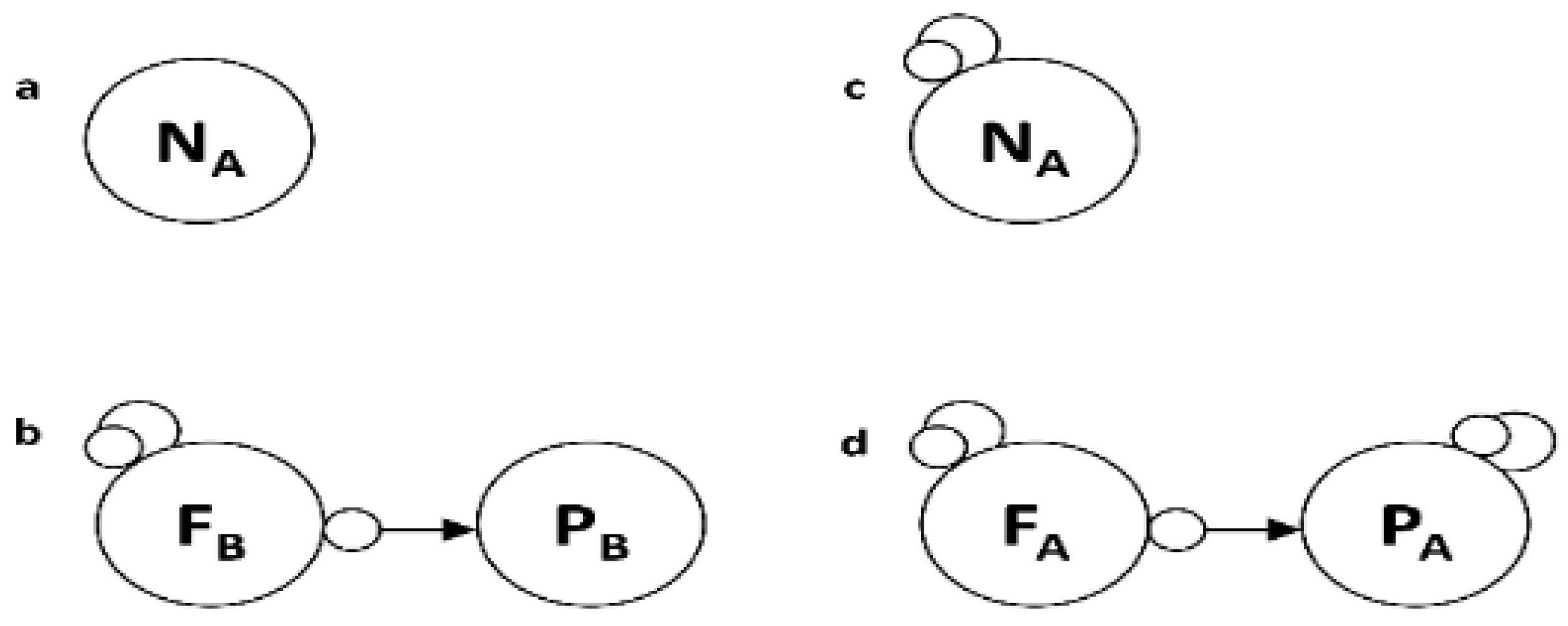
Figure 2.
Loop models of a six-node food chain. Nodes are depicted as large circles, and parameter inputs are shown as dark input arrowheads or circle heads. Lines, ending in small arrowheads, produce a positive effect on the nodes they touch, and circle heads produce a negative effect on the node they touch. Key to nodes: N=nutrient, A=algae, H=herbivores, M=meso-predator, F=small fish, and P=piscivore. A. The top predator is self-damped. B. The top predator is not self-damped. Predictions are given in Table 3.
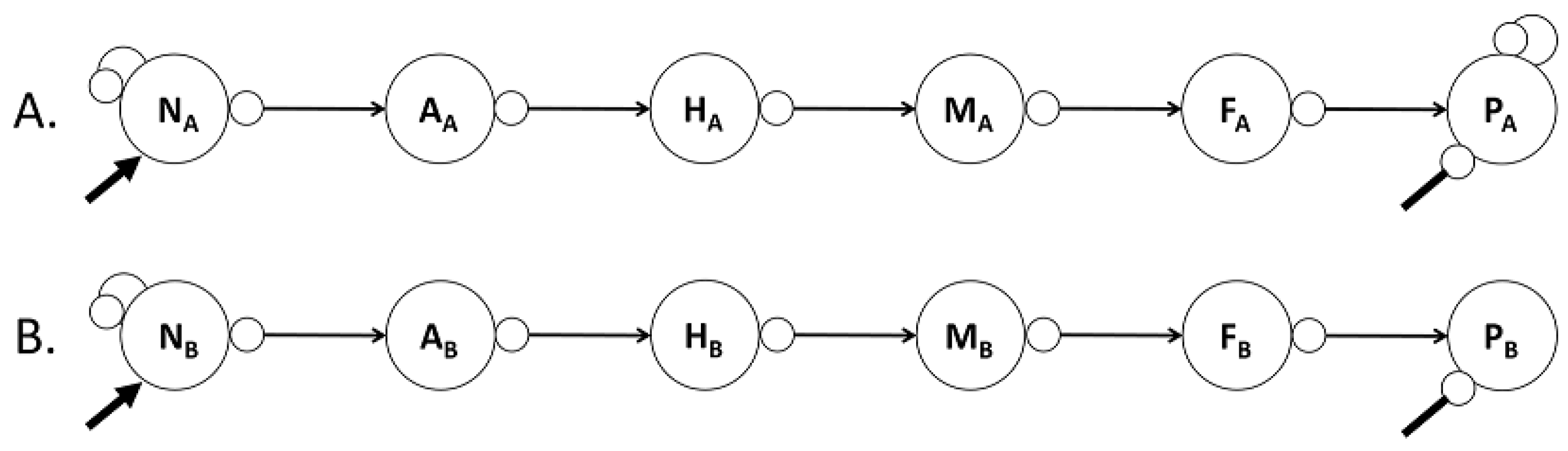
Figure 3.
Loop models of a six-node food chain with side links. Key to nodes: N=nutrient, A=algae, H=herbivores, M=meso-predator, F=small fish, and P=piscivore.
Figure 3.
Loop models of a six-node food chain with side links. Key to nodes: N=nutrient, A=algae, H=herbivores, M=meso-predator, F=small fish, and P=piscivore.
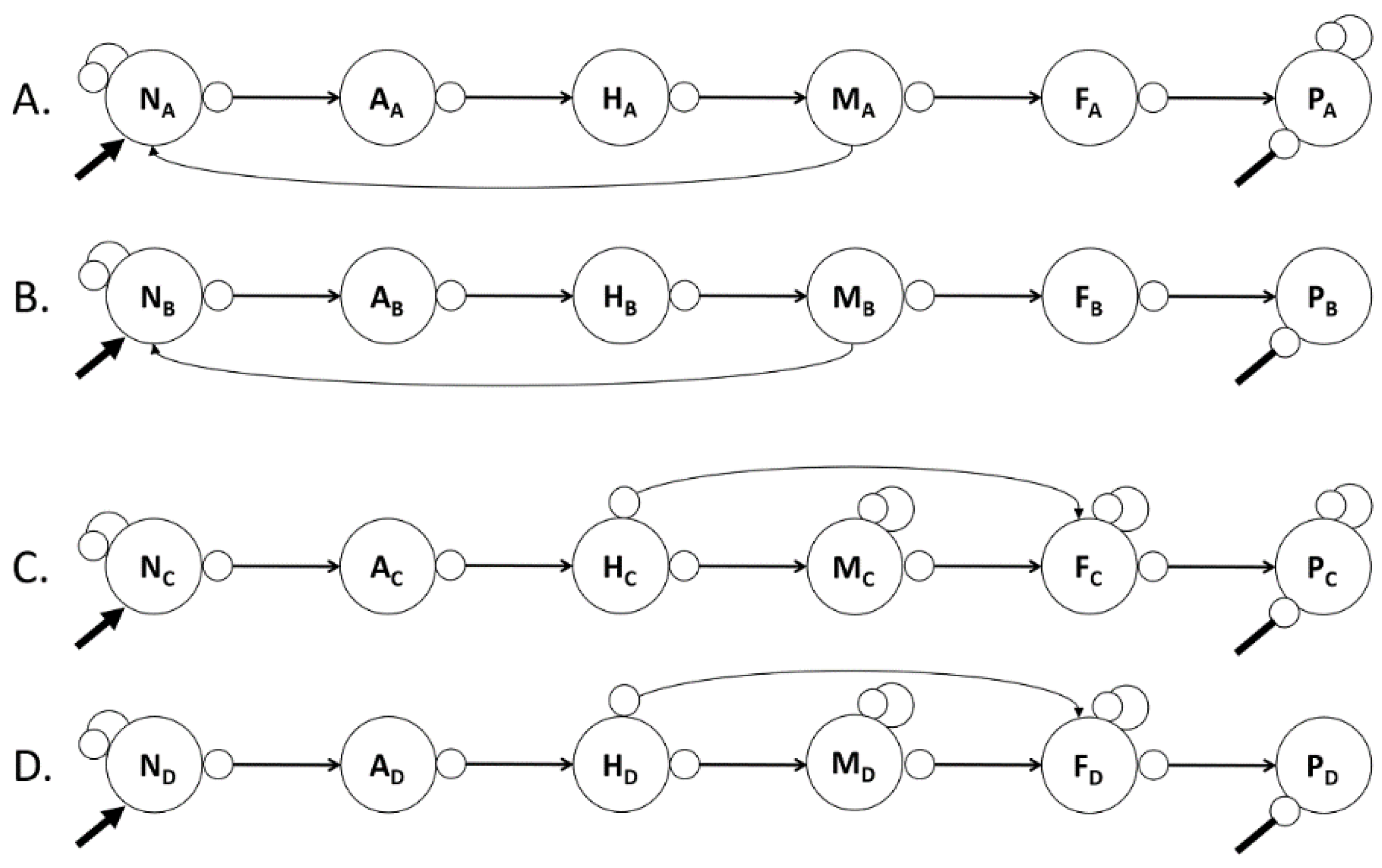
Figure 4.
Core Model of Several Marine Plankton Communities. This is a summary of four sets of food web models from the Delaware Bay, Narragansett Bay, and two mesocosms: the Marine Ecosystem Research Laboratory at the University of Rhode Island, located on the shores of Narragansett Bay, and the Dalhousie University Tower Tank in Halifax, Nova Scotia (Lane, 2018b). Key to nodes: Si=silica, N1=inorganic nitrogen/phosporus ratio, N2=organic nutrient pool, A1=diatoms, A2=dinoflagellates, A3=luxury consuming diatoms, A4=microflagellates, A5=monads and miscellaneous algae, A6=silica flagellates, Z1=adult copepods, Z2=immature copepods, Z3=adult copepods, Z4=cladocerans, O=Oikopleura spp. (tunicates), M=mollusc larvae, PC=polychaeta and cirriped larvae, D=decapod larvae, T=ctenophores, S=Sagitta spp. (chaetognaths), MD=hydromedusae, and A=anemonae larvae.

Figure 5.
Example of a random network of 21 nodes and 69 links, like Figure 4 Loop Model. .
Figure 5.
Example of a random network of 21 nodes and 69 links, like Figure 4 Loop Model. .
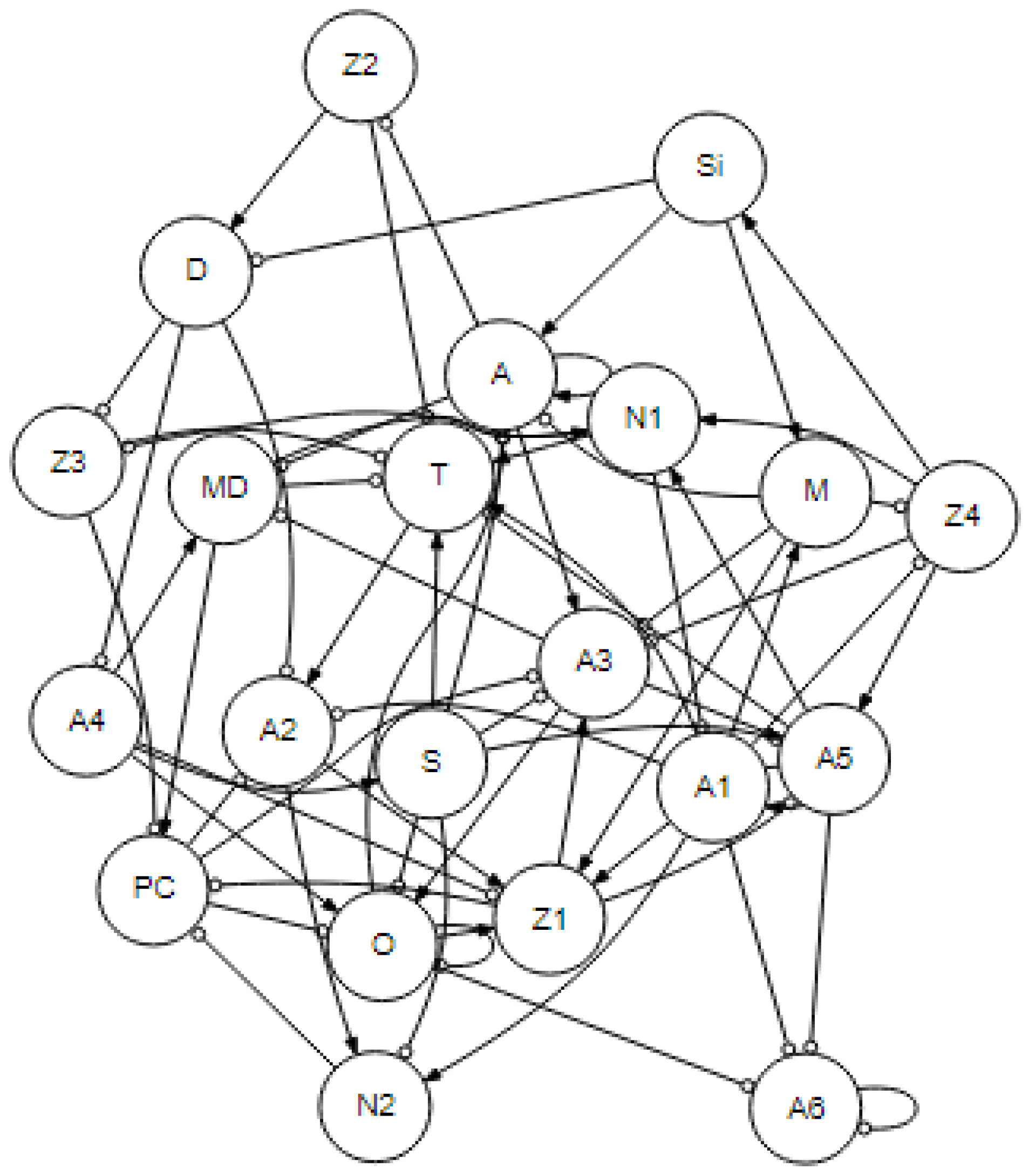
Figure 6.
Feedforward network motifs with three nodes. Motifs a-d are coherent since both pathways from NA to HA are of the same sign, and they reinforce each other. Motifs e-h are incoherent since the two pathways from NA to HA have opposite signs. Type 1 equals a and e, Type 2 equals b and f, Type 3 equals c and g, and Type 4 equals d and h.
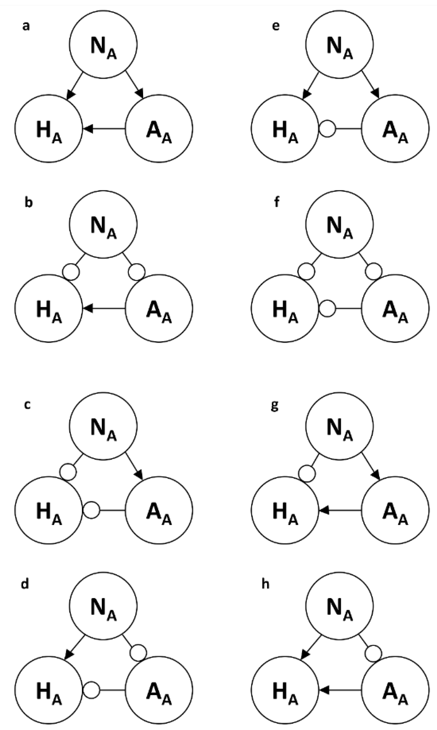
Table 1.
Overview of Definitional Considerations (C1-C4) for Ecological Control from a Single Species to a Food Web. Only a few possible examples of density changes are included. Each controller may internally change or be subject to the influence of an external driver, which is not part of the system. For a detailed explanation of changes for trophic pathways, see Lane (2017a,b). Key: b = birthrate and d = death rate.
| Controller (C1) |
Controlee (C2) |
Change (C3) |
Process (C4) |
|
|---|---|---|---|---|
| (1)Single Species A on Self | An external driver to A or A changing internally due to gene turning on or off, developmental process, etc. |
Species A | Species A exhibits changes in density with concurrent changes in birth or death rates. | Species A is activated or deactivated to cause morphological, physiological, behavioral, population etc. changes. |
|
(2) Two Species Interactions |
An external driver to A or A changing internally |
Species B: Prey |
Predator decreases prey density. | Predator A consumes Prey B (Predator ‘b’ increases) (Prey ‘d’ increases). |
| An external driver to B or B changing internally |
Species A: Predator | Prey increases predator density. | Prey B is consumed by Predator A. (Predator ‘b’ increases). |
|
|
(3) Trophic Pathway -Trophic Cascade (top-down) |
An external driver to Predator A or A changing internally A = Species or Functional Group A |
Nodes B & C or Functional Groups B & C on the pathway: A-B-C |
Densities change as: 0 0 0, + - + or - + - + - + or - + - |
Coupled biological interactions, especially predator-prey pairs of 3 or more nodes. |
| -Trophic Escalade (bottom-up) | An external driver to Prey C or C changing internally C = Species or Functional Group C |
Nodes C & B or Functional Groups C & B on the pathway: C-B-A |
Densities change as: 0 0 0, + + + or - - - 0 + 0 or 0 - 0 + 0 + or - 0 - |
Coupled biological interactions, especially predator-prey pairs of 3 or more nodes. |
| (4) Food web | Externally Perturbed Species or Functional Group or internally changing |
Other Food Web Components |
Densities of one or more nodes may change, or the whole food web structure can be altered. | External driver to one node can change all others through multiple pathways and feedback loops. A food web may undergo self-reorganization. |
Table 2.
Examples of drivers affecting ecological systems in context-independent and context-dependent situations across the biological hierarchy.
Table 2.
Examples of drivers affecting ecological systems in context-independent and context-dependent situations across the biological hierarchy.
| EXTERNAL DRIVERS | INTERNAL DRIVERS | |
|---|---|---|
| CONTEXT INDEPENDENT | ||
| One Species | A top predator experiences a favourable temperature change, causing it to increase its reproduction in a Q10 response. | |
| Two Species | An algal species poisons an herbivorous copepod, decreasing its abundance but not its position in the food web. | |
| Pathways: ≥ 3 Species | Rising light levels increase photosynthetic rates of phytoplankton, initiating a trophic escalade. | A top predator consumes several prey species, whose pattern of relative abundance is not maintained in the absence of the predator, resulting in a trophic cascade; however, the nodes and links remain intact. |
| Food Web | Abundances of food web nodes might change, but system identity and overall network configuration remains intact although system exhibits various behaviors. | |
| CONTEXT DEPENDENT | ||
| One Species | A pH change that exceeds a species’ tolerance level causes it to go locally extinct, thereby removing that node and all its links. | As some copepods develop from eggs to adults, their feeding habits change from herbivory to carnivory, and new food webs (or links) emerge. |
| Two Species | An invasive predator species becomes established in the food web, creating a new node with new links and local extinction of the original predator. | A top predator consumes a prey species to such low levels that it becomes locally extinct, and the system changes. |
| Pathways: ≥ 3 Species | Decreasing temperatures cause a decline in fish egg production, initiating a trophic cascade. |
|
| Food Web | Nodes and links are added or subtracted, thus changing food web structure. System identity does not remain intact. |
|
Table 3.
Community effects predictions for parameter inputs entering at the bottom (nutrient-Rows 1-4) and the top (predator-Rows 5-8) of a food chain producing trophic escalades (TEs) and trophic cascades (TCs) in Figures 2a and 2b. Key to nodes: N=nutrient, A=algae, H=herbivores, M=meso-predator, F=small fish, and P=piscivore. Row 1 should read that if there is a positive parameter input to NA, then N, A, H, M, F, and P all increase their standing crops. Each row contains one set of predictions for all nodes in the food chain. The prediction part of this table is a Community Effects Matrix.
PREDICTIONS 
|
|||||||||
|---|---|---|---|---|---|---|---|---|---|
| ROW NUMBER | TE or TC | FIGURE | PARAMETER INPUT | N | A | H | M | F | P |
| 1 | TE | 1a | +NA | + | + | + | + | + | + |
| 2 | TE | 1a | -NA | - | - | - | - | - | - |
| 3 | TE | 1b | +NB | 0 | + | 0 | + | 0 | + |
| 4 | TE | 1b | -NB | 0 | - | 0 | - | 0 | - |
| 5 | TC | 1a | -PA | + | - | + | - | + | - |
| 6 | TC | 1a | +PA | - | + | - | + | - | + |
| 7 | TC | 1b | -PB | + | - | + | - | + | - |
| 8 | TC | 1b | +PB | - | + | - | + | - | + |
Table 4.
Community effects predictions for parameter inputs entering at the bottom (nutrient-Rows 1-4) and top (predator-Rows 3-12) of a food chain producing trophic escalades (TEs) and trophic cascades (TCs) in Figures 3a and 3b. Key to nodes: N=nutrient, A=algae, H=herbivores, M=meso-predator, F=small fish, and P=piscivore. In this model, there is a one-way link change representing the invertebrate meso-predators (M) excretion of a large amount of bioavailable nitrogen to the nutrient stock (N), which affects trophic cascade predictions but not those of trophic escalades (Rows 1-4). * This indicates that when the parameter input affects P, there is a second pathway that goes from P-F-M-N-A-H in the trophic cascade predictions (Rows 5-12). ‘?’ indicates ambiguous predictions for two or more pathways for Rows 5-12. The prediction part of this table is a Community Effects Matrix.

Table 5.
Community effects predictions for parameter inputs entering at the bottom (nutrient: Rows 1-8) and top (predator: Rows 9-16) of a food chain producing trophic cascades (TCs) and trophic escalades (TEs) in Figures 2C and 2D. Key to nodes: N=nutrient, A=algae, H=herbivores, M=meso-predator, F=small fish, and P=piscivore. ‘?’ indicates ambiguous predictions for two or more pathways. * represents a potential second pathway, N-A-H-F-M, for Tes. ** indicates that when the parameter input affects P, there is a third pathway that goes from P-F-H-M for trophic cascades. The prediction part of this table is a Community Effects Matrix.
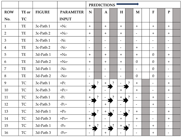
Table 6.
Number of Pathways (Operating and Non-operating)and Feedbacks Per Level (1-21) for an Ecological Skeleton Loop No. 16. L = number of links in a path, and N = number of nodes in a feedback loop. For loops, but not paths, the numbers of nodes and links are the same since the loop returns to the starting node.
| Loop Length | Operating Paths |
Non-operating Paths |
Total Paths |
N | Negative Feedback Loops |
Positive Feedback Loops | Total Feedback Loops |
|---|---|---|---|---|---|---|---|
| 1 | 54 | 0 | 54 | 1 | 15 | 0 | 15 |
| 2 | 137 | 4 | 141 | 2 | 25 | 0 | 25 |
| 3 | 297 | 10 | 307 | 3 | 5 | 3 | 8 |
| 4 | 552 | 27 | 579 | 4 | 0 | 10 | 10 |
| 5 | 933 | 44 | 977 | 5 | 1 | 7 | 8 |
| 6 | 1376 | 53 | 1429 | 6 | 8 | 7 | 15 |
| 7 | 1682 | 40 | 1722 | 7 | 12 | 2 | 14 |
| 8 | 1631 | 38 | 1669 | 8 | 3 | 3 | 6 |
| 9 | 1322 | 20 | 1342 | 9 | 0 | 2 | 2 |
| 10 | 802 | 9 | 811 | 10 | 0 | 0 | 0 |
| 11 | 378 | 0 | 378 | 11 | 0 | 0 | 0 |
| 12 | 121 | 0 | 121 | 12 | 0 | 0 | 0 |
| 13 | 28 | 0 | 28 | 13 | 0 | 0 | 0 |
| 14 | 0 | 0 | 0 | 14 | 0 | 0 | 0 |
| 15 | 0 | 0 | 0 | 15 | 0 | 0 | 0 |
| 16 | 0 | 0 | 0 | 16 | 0 | 0 | 0 |
| 17 | 0 | 0 | 0 | 17 | 0 | 0 | 0 |
| 18 | 0 | 0 | 0 | 18 | 0 | 0 | 0 |
| 19 | 0 | 0 | 0 | 19 | 0 | 0 | 0 |
| 20 | 0 | 0 | 0 | 20 | 0 | 0 | 0 |
| 21 | 0 | 0 | 0 | 21 | 0 | 0 | 0 |
| Total | 9313 | 245 | 9558 | Total | 69 | 34 | 103 |
Table 7.
Community effects matrix for No. 16 Ecological Skeleton shown in Figure 4 with zooplankton links (d and e). Read predictions for changes in standing crops across a row for a positive driving force to the left-hand node in each row. Key to nodes: Si=silica, N1=inorganic nitrogen/phosporus ratio, N2=organic nutrient pool, A1=diatoms, A2=dinoflagellates, A3=luxury consuming diatoms, A4=microflagellates, A5=monads and miscellaneous algae, A6=silica flagellates, Z1=adult copepods, Z2=immature copepods, Z3=adult copepods, Z4=cladocerans, O=Oikopleura spp. (tunicates), M=mollusc larvae, PC=polychaeta and cirriped larvae, D=decapod larvae, T=ctenophores, S=Sagitta spp. (chaetognaths), MD=hydromedusae, and A=anemonae larvae.
| Si | N1 | N2 | A1 | A2 | A3 | A4 | A5 | A6 | Z1 | Z2 | Z3 | Z4 | A | D | M | MD | O | PC | S | T | |
| +Si | + | - | + | - | - | + | - | - | + | + | + | + | - | - | - | - | + | - | - | + | + |
| +N1 | - | + | - | + | + | - | + | + | - | - | - | - | + | + | + | + | - | + | + | - | - |
| +N2 | - | - | + | - | + | + | - | - | - | - | - | - | - | + | + | + | - | - | - | - | - |
| +A1 | ? | ? | ? | + | ? | - | ? | ? | ? | ? | ? | ? | ? | ? | ? | ? | ? | ? | + | ? | ? |
| +A2 | - | - | - | - | + | + | - | - | - | - | - | - | - | + | + | + | - | - | - | - | - |
| +A3 | - | - | + | - | - | + | - | - | - | + | + | + | - | - | - | - | + | - | - | + | + |
| +A4 | + | - | + | - | - | + | + | - | + | + | + | + | - | - | - | - | + | + | - | + | + |
| +A5 | + | - | + | - | - | + | - | + | + | + | + | + | + | - | - | - | + | - | - | + | + |
| +A6 | - | + | - | + | + | - | + | + | + | - | - | - | + | + | + | + | - | + | + | - | - |
| +Z1 | + | + | - | + | + | - | + | + | + | + | - | - | + | + | + | + | - | + | + | - | + |
| +Z2 | + | + | + | - | - | + | + | + | + | + | + | + | + | + | + | - | + | + | - | + | + |
| +Z3 | + | + | + | + | - | - | + | + | + | + | + | + | + | + | + | - | + | + | + | + | + |
| +Z4 | - | + | - | + | + | - | + | - | - | - | - | - | + | + | + | + | - | + | + | - | - |
| +A | ? | + | ? | + | ? | - | - | + | + | - | + | - | + | + | - | - | - | - | + | - | - |
| +D | + | + | + | + | - | - | + | + | + | + | + | + | + | - | + | - | + | + | + | + | + |
| +M | - | - | + | - | - | + | - | - | - | - | - | - | - | - | - | + | - | - | - | - | - |
| +MD | - | - | - | - | + | + | - | - | - | - | - | - | - | - | - | + | + | - | - | - | - |
| +O | - | + | - | + | + | - | - | + | - | - | - | - | + | + | + | + | - | + | + | - | - |
| +PC | - | - | - | + | + | + | - | - | - | - | - | - | - | + | + | - | - | - | + | - | - |
| +S | - | - | - | - | + | + | - | - | - | - | - | - | - | - | - | + | - | - | - | + | - |
| +T | - | - | + | - | - | + | - | - | - | - | + | + | - | - | - | - | + | - | - | + | + |
Table 8.
Listing of Network Properties and Potential Internal Constraints for Marine Food Webs Key: NEI=Nutrients, Energy, Information.
Table 8.
Listing of Network Properties and Potential Internal Constraints for Marine Food Webs Key: NEI=Nutrients, Energy, Information.
| Potential Ecosystem Chimera Functions | |||
|---|---|---|---|
| Structure & Function | Secure NEI: Nutrients, Energy, Information | Maintain Modular Identity/Stability | Manage Time |
| 3-Tier Lattice | Built around nutrient input nodes, contains nine nodes most likely to receive environmental drivers and occur as high-frequency links and paths. Accommodates a complete set of feeding types. |
Helps form modular patterns and shapes; lattices are robust structures common in in biological hierarchies. Could be 3-dimensional in nature. Lattice structures are known to be robust in other contexts. |
Lattice structure shortens the time for energy, nutrient, and information flows among the nine key nodes. Promotes a scaffolding in terms of key temporal relationships. |
|
Valid Complement Rule |
Determines the flows of NEI by distinguishing operating from non-operating paths |
Constraints the behavior of nodes not on the path into a set of disjoint loops. | All nodes are slotted into temporal paths and cycles synchronously for each time dominated by an external driver. |
| Stability Rules- Routh-Hurwitz Criteria | Closed loops facilitate recycling and material economies. | Overall pattern of feedback loops, including their lengths and signs, ensures network stability when there is a prevalence of short negative loops versus long positive ones. |
Each feedback loop takes a given amount of time to traverse all its nodes and return to the starting node. Generally, longer loops take longer than short ones. |
| Non-linear Focal Points | Assists in the choice of pathways on which to move nutrients, energy, and information. | Provides the flexibility so that the main lattice module can undergo topological stretching without breaking. |
Gives time management flexibility through the coordination of life history stages. |
|
Satellite Nodes |
Turn pathways on and off as a function of the satellite's self-damping. | Self-damping adds to overall network stability. | As a result of the time given, the satellite will only be self-damped at high densities in an annual cycle. |
|
Network Motif: Auto-regulation |
Keeps nutrients in a steady state, which is often observed in marine environments. |
Central stabilizer in food webs. Helps balance longer positive loops. | Significantly affects temporal relationships. |
|
Network Motif: Feedforward 3 nodes |
Could provide security as well as change NEI rates as conditions warrant. |
Provides path choice, which has temporal ramifications. | It is the primary source of anticipation and can speed up critical interactions. |
|
Network Motif: Bi-fan/Parallel 4 nodes |
Provides pathway flexibility, perhaps increasing security. |
It could help in maintaining stability. | Unclear |
Disclaimer/Publisher’s Note: The statements, opinions and data contained in all publications are solely those of the individual author(s) and contributor(s) and not of MDPI and/or the editor(s). MDPI and/or the editor(s) disclaim responsibility for any injury to people or property resulting from any ideas, methods, instructions or products referred to in the content. |
© 2025 by the authors. Licensee MDPI, Basel, Switzerland. This article is an open access article distributed under the terms and conditions of the Creative Commons Attribution (CC BY) license (http://creativecommons.org/licenses/by/4.0/).
Copyright: This open access article is published under a Creative Commons CC BY 4.0 license, which permit the free download, distribution, and reuse, provided that the author and preprint are cited in any reuse.


