

Submitted:
28 July 2025
Posted:
29 July 2025
You are already at the latest version
Abstract
Prototype-Based Networks (PBNs) are inherently interpretable architectures that facilitate understanding of model outputs by analyzing the activation of specific neurons —referred to as prototypes—during the forward pass. The learned prototypes serve as transformations of the input space into a latent representation that more effectively encapsulates the main characteristics shared across data samples, thereby enhancing classification performance. Crucially, these prototypes can be decoded and projected back into the original input space, providing direct interpretability of the features learned by the network. While this characteristic marks a meaningful advancement toward the realization of fully interpretable artificial intelligence systems, our findings reveal that prototype representations can be deliberately or inadvertently manipulated without compromising the superficial appearance of explainability. In this study, we present a series of empirical investigations that substantiate this phenomenon and introduce it as a structural paradox inherent to the architecture itself, which may pose a significant robustness concern for explainable AI methodologies.
Keywords:
Prototype-Based Networks
; Interpretable AI
; Robustness of Explanations
; Neural Networks
1. Introduction
Model interpretability is a critical requirement in the development of machine learning models intended to represent aspects of real-world phenomena. Numerous techniques and studies have sought to enhance interpretability, primarily through post hoc analyses or by employing surrogate models that are inherently more interpretable. Despite these efforts, a fundamental challenge persists: establishing a clear correspondence between the knowledge acquired by the model and observable elements of reality. In an effort to address this issue, a Prototype Deep Neural Network (PDNN) was introduced in [1]. Prototype learning is a subclass of intrinsically interpretable methods, derived from the classical paradigm of case-based reasoning known as prototype classification. In this context, a prototype is not constrained to a single observation from the training set, but rather may constitute a generalized representation formed from a combination of multiple samples in the learned latent space [2]. The prototype learning framework typically incorporates an autoencoder in conjunction with a prototype classifier layer. The autoencoder generates a compressed latent representation of the input data, while the prototype layer identifies representative points within this space that both resemble specific inputs and are indicative of particular classes. Each learned prototype can subsequently be visualized through the decoder, enabling interpretability of the learned features, and can be traced back to the output softmax layer, thereby providing insight into class associations. Moreover, this architectural design supports a form of case-based reasoning by identifying the training sample(s) most similar to a given prototype, further enhancing the transparency and accountability of the model’s decision-making process.
In this context, while the interpretability of the method has received considerable attention, the reliability and validity of the learned prototypes have often been overlooked. For relatively simple datasets, such as handwritten digits [3], prototype validation is typically performed by reconstructing and visualizing the prototypes in the input space, followed by a qualitative assessment of whether the prototypes visually resemble the intended classes. However, this raises a critical question: can we confidently assert that a prototype which appears to represent, for instance, the digit ‘1’, is indeed interpreted as such by the deep neural network (DNN)? In this study, we address this question through a series of experiments, including the development of a novel Deep Prototype-Based Network. Our results demonstrate that visual similarity does not necessarily align with the model’s internal representation, highlighting a potential gap between human interpretability and model-driven classification.
2. State of the Art
[4] were the first to show that deep networks can reason through learned prototypes while remaining end-to-end trainable. Prototype-based neural networks offer a hybrid approach that combines the power of deep learning with the interpretability of case-based reasoning. Its architecture integrates a convolutional autoencoder with a prototype-based classification layer, allowing the model to explain its predictions through comparisons with prototypical training examples. Building upon this foundational work, [5] proposed ProtoPNet, a model that popularized the "this-looks-like-that" paradigm through patch-to-prototype visualizations. The training methodology incorporated techniques such as prototype projection and class-specific weight regularization, achieving competitive performance across fine-grained classification tasks involving bird, car, and dermatological image datasets, while preserving interpretable, image-level justifications.
Two primary strategies have been proposed to overcome the representational limitations inherent in single-layer prototype-based models. First, [6] introduced ProtoTree, a differentiable decision tree architecture in which internal nodes correspond to learned prototypes. This structure enables an input to traverse only nodes, producing compact and interpretable rule chains. Second, explicit prototype hierarchies [7] organize low-level visual parts into increasingly abstract semantic concepts, facilitating multi-granular reasoning and enhancing robustness to out-of-distribution inputs.
Hybrid approaches have also been developed to enable reasoning beyond raw pixel representations. Concept Bottleneck Models (CBMs) [8] structure the prediction pipeline around human-interpretable attributes, allowing users to intervene and correct misclassified concepts at inference time. In a complementary direction, the Deep k-Nearest Neighbours (DkNN) algorithm [9] enhances arbitrary classifiers by incorporating layer-wise nearest neighbor retrieval, thereby quantifying model uncertainty through non-conformity scores. Both methods underscore the utility of leveraging intermediate representations, particularly similarity structures within hidden layers, without compromising predictive accuracy, a principle that underpins the multi-layer prototype architecture proposed in this work. Additionally, Capsule Networks [10] implement dynamic routing mechanisms to capture part-to-whole relationships, while part-based R-CNNs [11] localize discriminative object regions.
The Deep Prototype Network (DPN) introduced in this work adopts a compositional reasoning framework akin to prior hierarchical or part-based models, but implements this structure through a deliberately layered architecture rather than relying on post hoc clustering of prototypes. This design choice is motivated by the principle that successive prototype layers should progressively capture increasingly abstract semantic concepts or larger spatial extents, thereby enabling richer part-to-whole reasoning directly within the network’s forward pass.
3. Deep Prototype-Based Network Architecture
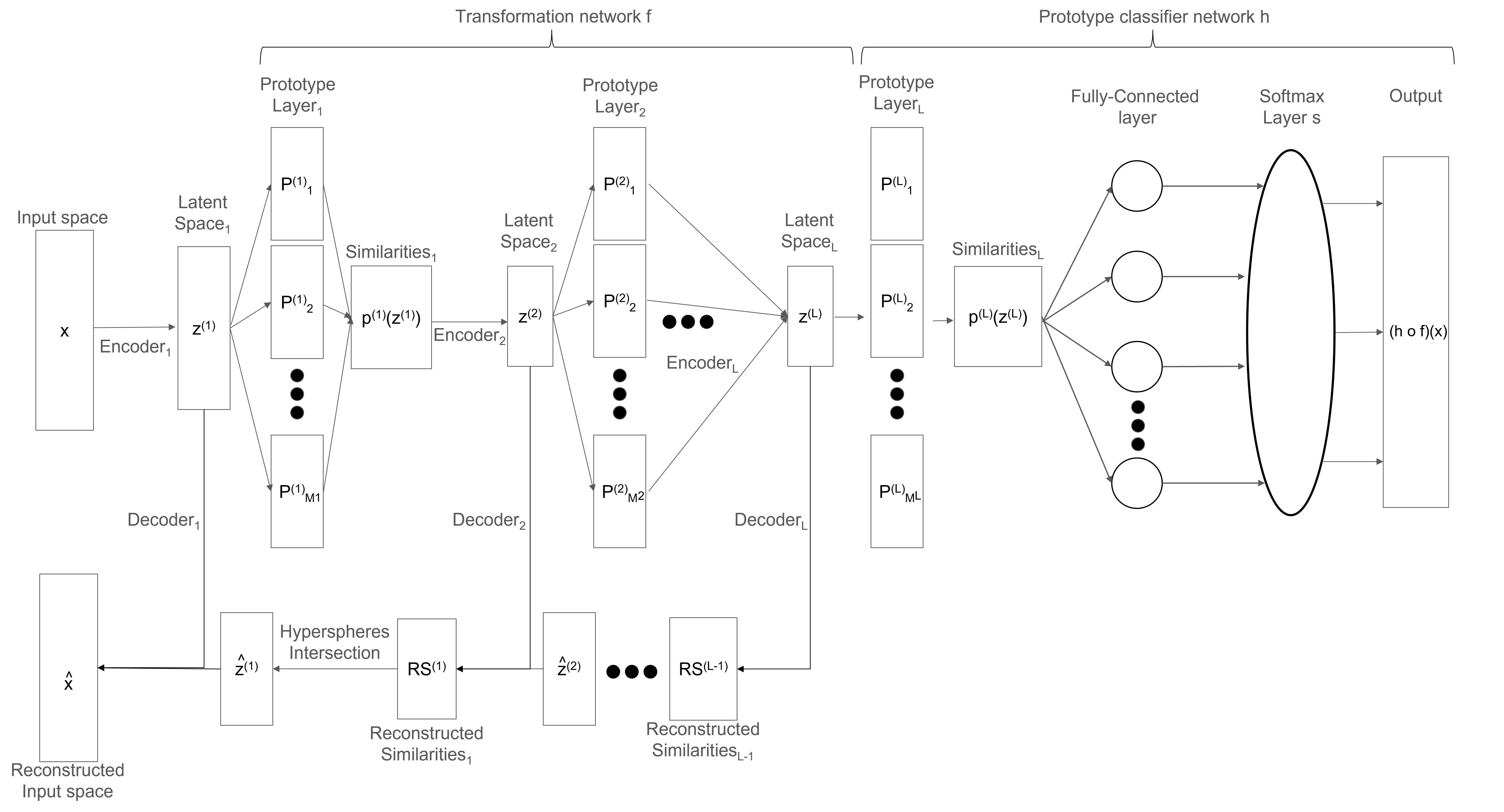
Figure 1 illustrates the proposed Deep Prototype-Based Network (DPBN) architecture, which extends Li et al. [2018]’s notation, cost terms, and design philosophy, but stacks several prototype layers in a feedforward chain rather than using a single one. This architecture performs a back-and-forth data flow that couples representational capacity with prototype-based interpretability.
Let , , denote a finite training set sampled from an underlying distribution . All spaces are Euclidean and, therefore, equipped with the canonical inner product and the induced norm . The uppercase calligraphic symbols note sets or spaces, and the superscripts in parentheses index the depth . The set of all network parameters is denoted as .
3.1. The Forward Encoding Flow
The upper part of Figure 1 shows that the forward flow begins in the input space, followed by the first encoder, which maps the input data to a latent space. Then, the transformation network f comprises L-1 stacked triples consisting of a prototype layer, the calculation of a similarity vector, and an encoder for the following layer. Finally, the prototype classifier network h takes as input the last prototype layer (L), calculates the similarity vector, and passes the results through a linear mapping with a subsequent softmax layer that produces the estimated classification distribution of an input.
The input space domain is a subset of a p-dimensional real vector space. A sample is denoted by x . No further structure is assumed, except for the differentiability of all subsequent mappings defined on .
The first layer of the DPBN is the first encoder, which projects input data onto a lower-dimensional manifold:
The mapping is usually implemented using a convolutional neural network that ends with a fully connected layer of width . The parameters associated with this mapping are collectively denoted by and form part of the general parameter set.
The next layer is the first prototype layer ,
and comprises a finite set of prototypes. The value is a fixed hyperparameter a priori, while prototypes are learned during the training process. Given a latent representation , its similarity vector is calculated using the squared Euclidean distance to all prototypes. It is collected in the similarity vector
which defines differentiable functions , thereby enabling the application of gradient-based optimization methods without requiring any modifications.
The next layer is the second encoder. The resulting similarity vector computed in the previous layer, which does not contain any positional ordering, is compressed by a learned distance encoder to obtain the second layer representation.
The function is implemented as a multilayer perceptron, with its parameters collectively denoted by . The representation can be expressed as using the composition of functions.
Similarly to the first layer, for every subsequent layer , there is an encoder that generates the latent space , followed by a prototype set , then a similarity vector , and finally an encoder for the next layer :
We denote as the composite mapping that transforms x into .
To provide the final classification decision after passing through all layers of the DPBN, the final similarity vector is fed into a linear map to obtain
The subsequent softmax activation function produces the estimated class distribution , where is the predicted class.
A summary of the forward flow from the input vector x to the predicted class distribution is as follows:
3.2. The Backward Decoding Flow
What distinguishes prototype-based networks, and in particular the proposed DPBN, from regular neural networks is the presence of prototypes that, through their reconstruction back into the input space, offer visual explanations for their predictions. However, this visualization is not straightforward in the case of the DPBN. The procedure to visualize deeper prototypes introduces a novel approach called the hypersphere intersection (HS-Int) algorithm, which transforms a reconstructed similarity vector at deep ℓ, in Figure 1 or , into a reconstructed code .
The lower part of Figure 1 shows the backward decoding flow that reconstructs the deepest code back into the input space. This reconstruction process performs L-1 decoding and hypersphere-intersection pairs until obtaining the first reconstructed code . Finally, is decoded back into .
The hypersphere intersection algorithm is based on previous results from algebraic and geodesy/GPS positioning [12,13,14], as well as nonlinear least-squares optimization (Levenberg-Marquardt) [15,16] and the Moore-Penrose generalized inverse matrix theory [17,18].
For any depth , the decoder produces the radius vector
which, together with the prototype set , defines hyperspheres in the ambient space as follows:
where and to simplify the notation. Thus, the objective becomes to recover a point or, if the intersection is empty, the solution to the minimization problem
We draw on previous studies in this field to design the algorithm in three steps. The first is to perform linear reduction by applying Bancroft’s algebraic difference trick [12] to obtain the linear system:
Its least-squares solution is , where is the Moore-Penrose pseudoinverse. Every other solution differs from by an element of the null space of A:
where represents the rank of matrix A, N stacks an orthonormal basis of , with being the kernel of matrix A, so d equals the number of remaining degrees of freedom and are their coordinates. If , the linear part has isolated at most one candidate; otherwise, the quadratic constraint of the next step must fix (or show that there is no exact intersection).
The second step inserts the above-mentioned parameterization into the first sphere equation , which yields
If , no free parameters remain, and q reduces to a constant; the unique linear candidate is an exact intersection; otherwise, no actual solution exists.
If , then is an ordinary quadratic in one variable. Its roots have closed forms tabulated by Norrdine [14, Alg. 2], producing up to two exact points, which we collect in .
Lastly, if , then it means that the same equation defines at most a -dimensional quadric in the space. Therefore, we launch a Levenberg-Marquardt search [16] from to find a feasible (or certify that none exists), following Norrdine’s least squares recipe [14, Alg. 1].
Finally, any that satisfies is mapped through and added to in the third step. However, if no exact intersection is found, (), we minimize the nonlinear least-squares cost
The optimization process uses the Levenberg-Marquardt-damped Gauss-Newton scheme [15,16], which smoothly interpolates between gradient descent and the Gauss–Newton step via an adaptive damping factor. After convergence, we obtain . The local uniqueness is verified with the Jacobian rank criterion of Abel-Chaffee [13]. The algorithm finally returns together with the uniqueness flag.
Once the HS-Int algorithm is described, we can define the decoding cascade, which starts from , applies a decoding step
and then applies the HS-Int algorithm
to . Note that the decoding step transforms a code from a latent space into a reconstructed similarity vector. Then, the HS-Int algorithm takes the reconstructed similarities vector and the set of prototypes from the corresponding prototype layer to generate the reconstructed code for the previous layer. Finally, is the global reconstruction against which the reconstruction term in (2) is measured. This cascade enforces explicit geometric consistency between successive latent spaces, endowing every latent point with a deterministic pre-image in the input domain.
The reconstruction pathway can be summarized as
The proposed DPBN provides expressive capacity and interpretability. Every depth applies the composition , which is Lipschitz continuous when employs bounded activation functions, endowing the network with a hierarchical piecewise-smooth warping of the latent metric. Yet interpretability is preserved: each prototype is deterministically mapped to the input domain by the reconstruction chain, which yields a visual or otherwise perceptible exemplar representing that prototype at its innate semantic granularity.
3.3. Guided Prototype Learning
Together with the pipelines for classification and decoding, it is crucial to define the joint learning objective of the network architecture.
Let be the cross-entropy between the prediction and the ground truth y. With referring to the latent codes of a mini-batch of size B, we define the layer-wise prototype coverages as:
Similarly, with a mini-batch of size B, we establish the loss functions of the autoencoders for the image and the distances as:
As such, for positive scalars acting as regularization terms , , , and , the total loss reads
All model parameters are trained by stochastic gradient descent on (2), with gradients obtained via automatic differentiation through the analytic Jacobian of HS−Int whenever the exact intersection is unique; otherwise, the sub-gradient of the best-fit residual is used.
4. Experiments and Results
In this section, we conduct a systematic evaluation of the proposed Deep Prototype-Based Network (DPBN), complemented by a series of targeted architectural variants. This analysis aims to demonstrate the model’s capabilities while also addressing a key challenge: the tension between visually interpretable prototype reasoning and the internal mechanisms of class assignment within the network.
The first is a baseline experiment to assess performance on the MNIST dataset ( [3]) and to examine the prototype representations obtained from the proposed DPBN architecture (see Figure 1). The second experiment is a model distillation study in which we investigate whether the prototypes learned by the deepest layer of a four-layer Deep Prototype-Based Network (DPBN) can be effectively transferred to a significantly shallower model, without compromising either predictive performance or interpretability. The third experiment addresses a binary classification task designed to demonstrate that the network can produce accurate predictions and visualizations consistent with the class "0", while its internal explanatory mechanisms align more closely with class "1".
For each experimental configuration, we report both classification accuracy and a novel validation metric introduced in this study—the Normalized Negative Entropy (NNE) score. Quantitative findings are further supported by qualitative analyses, comprising visualizations of reconstructed prototypes and learned weight matrices. Collectively, the results elucidate the impact of each architectural choice on the reliability, interpretability, and overall performance of DPBNs.
All the experiments are conducted using the MNIST( [3]) benchmark dataset. The original training set, comprising 60,000 images, is randonmly partitioned into for training and for validation. The official test set of images is held out for evaluation. All images are resized to pixels and normalized to the range using min-max scaling.
4.1. NNE Score
Prototype-based networks typically conclude with a linear classifier, where the weight matrix maps prototype–sample distances to class logits. To assess the interpretability of this final classification layer, we introduce the Normalized Negative Entropy (NNE) score. This metric interprets the prototype-to-class weight matrix W as an information-theoretic channel. After negating W, a row-wise softmax is applied to obtain a class probability distribution for each prototype. The Shannon entropy of each distribution is then computed, inverted, normalized by , and averaged across all prototypes. The resulting NNE score lies within the interval , attaining a maximum value of 1 only when each prototype exhibits a one-hot (i.e., perfectly class-specific) voting pattern.
In contrast to geometric alignment measures—such as the B-Cos transform [19], which enhances the fidelity of saliency maps by maximizing cosine similarity between inputs and classifier weights, or the support-vector-based alignment strategy employed by WASUP [20]—the NNE metric exclusively captures the distributional sharpness of the classification head, providing a complementary perspective on model interpretability.
Because large negative distances should yield a high vote, we first negate the weight matrix and apply a row–wise softmax:
Each row can now be read as a categorical distribution over classes for prototype i. As such, for a row we can compute its Shannon entropy
and normalise it by the maximum possible entropy to obtain a confidence score
when is a one–hot vector (prototype decisively represents one class) and when is uniform (prototype conveys no class information).
Finally, we average over all P prototypes:
is therefore higher for more interpretable weight matrices.
We validated the metric with two extreme cases:
| Matrix | NNE |
| Identity (perfectly sharp) | |
| Uniform (fully diffuse) |
It complements structural sparsity metrics such as global/local size and Hoyer–Square norms in ProtoS-ViT [21] and the “transparent-head complexity’’ of Shallow-ProtoPNet [22] by quantifying decisiveness even when the head is dense. Where neuron-level Class-Selectivity Indices normalize entropy over activations [23], NNE is the first to apply an entropy normalization directly to prototype voting weights, making it agnostic to input distribution and layer depth. Recent analyses of classifier weight spectra, enabled by bilinear multilayer perceptrons (MLPs) [24], underscore the value of interpreting the classification head as an information-theoretic channel. In this context, the NNE score provides a concise, task-size-invariant metric that aligns with and supports this perspective.
The proposed metric will be employed throughout this work to evaluate the quality of the classification weight matrix across all experiments, serving as a means to assess and compare the reliability and class specificity of the learned prototypes.
4.2. Experiment 1: Baseline Architecture
The objective of this experiment is twofold: to evaluate the performance of the proposed architecture on the MNIST dataset and to analyze the structure of the resulting prototype representations. As an initial step, we consider the canonical Deep Prototype-Based Network (DPBN), which closely follows the configuration introduced by [4], with minor modifications to facilitate subsequent ablation studies. The input pipeline preserves the original luminance pixel values of the MNIST digits, thereby avoiding information loss during preprocessing.
Within the network, layer 1 comprises compact convolutional encoder–decoder module that projects each input image into a 40-dimensional latent vector and reconstructs it back into pixel space. The encoder employs a fixed stride pattern of and a sequence of convolutional filters , progressively reducing the spatial resolution from to over four downsampling stages. This architectural design ensures that each spatial location in the final feature map corresponds to a roughly square receptive field in the input image, a property leveraged in later experiments to interpret prototype activations in a spatially meaningful manner.
The flattened feature map is subsequently projected into a latent representation of dimension via a fully connected layer. The choice of is deliberate, as it constrains the image autoencoder to learn a non-trivial, low-dimensional manifold rather than approximating the identity mapping. This serves as an implicit regularization mechanism for the initial prototype search space. Within this space, prototypes are allocated, resulting in a prototype-to-latent ratio of . Empirical observations from preliminary experiments indicated that this ratio is sufficient to support a near one-to-one correspondence between digit classes and prototypes, while avoiding the introduction of redundant representations.
The subsequent layers (layers 2 through 4) share an identical structural design, differing from the initial layer primarily in that their encoders are implemented as multilayer perceptrons (MLPs) operating on similarity vectors rather than raw image data. Specifically, each distance vector produced by layer l is projected into a latent space of dimension , , then decoded back to its original dimensionality , and subsequently passed to the next prototype layer of equal size. In each layer, the prototypes are initialized from a uniform distribution and jointly optimized alongside the corresponding autoencoder weights. Importantly, we enforce the condition at every depth to ensure that the resulting distance matrices are overcomplete -a necessary property for the hypersphere-intersection solver used to reconstruct prototype representations across layers.
The coefficients we set to based on a coarse log-grid search aimed at balancing classification accuracy with reconstruction fidelity. Model training was performed using the Adam optimizer with a fixed learning rate of 1e-4. An early stopping criterion with a patience of 100 epochs was employed, terminating training when validation accuracy failed to improve over 100 consecutive epochs. On the MNIST dataset, the model converged to a test accuracy of 98.05% after approximately 850 epochs, thereby establishing a strong performance upper bound for the ablation studies that follow.
Interpretability, however, diminishes with increasing network depth. As illustrated in Figure 2, reconstructed prototypes from all four layers are visually compared. Prototypes in the first layer exhibit clearly defined glyphs, each distinctly associated with a specific digit class. This observation confirms that the autoencoder, in conjunction with the terms regularization terms, effectively aligns prototypes with the underlying data manifold. By the layer 2, the prototypes lose fine-grained details and become more abstract, although they still retain rough class-specific contours. In layers 3 and 4, interpretability degrades substantially: the reconstructed shapes converge into nearly indistinguishable forms, differentiated only by subtle intensity variations and with weakly class-informative interpretable patterns. Despite this loss in human interpretability, the softmax-normalized weight matrix yields a Normalized Negative Entropy (NNE) score of 0.26, indicating that the classifier maintains a coherent and class-specific internal representation, even as the prototypes themselves become less visually discernible. This observation is particularly significant, as it indicates that the final-layer prototypes retain sufficient information to support accurate classification while simultaneously integrating multiple visual patterns. This behavior is a consequence of the decreasing dimensionality across successive layers, which compels the network to fuse lower-level features. Accordingly, the process can be interpreted as a hierarchical compositional mechanism that preserves discriminative attributes across layers.
4.3. Experiment 2: Model Distillation
In this experiment we investigate whether the prototypes learned by the deepest layer of a four-layer DPBN could be effectively transferred to a significantly shallower model without compromising either predictive accuracy or interpretability. Specifically, the prototype layer extracted from the fourth layer of the reference DBPN was copied into a single-layer DPBN, where it remained fixed during training. Only the autoencoder and the classification head were subsequently trained. Qualitative comparisons between the original layer-4 prototypes and those reconstructed by the distilled model, along with the associated weight matrices and , are shown in Figure 3 and Figure 4.
Despite the substantial reduction in network depth, the distilled model achieved an accuracy statistically indistinguishable from that of the baseline. Moreover, its weight matrix maintained coherence, with a NNE of 0.18. To assess whether this performance could be attributed to the information encoded in the transferred prototypes, we repeated the experiment using randomly initialized prototype vectors, which were likewise frozen during training. Contrary to our initial hypothesis, the network again attained comparable accuracy and produced sharply defined reconstructed prototypes. This suggests that the raw numerical values of the prototypes, in isolation, contribute little semantic content. Rather, interpretability appears to arise from the dynamics of the autoencoder and the spatial configuration of the prototypes within the latent space. Notably, the geometry of this space retains semantic structure: prototypes corresponding to visually similar digits, such as 8 and 9, are positioned closely, whereas those representing semantically distant digits, such as 2 and 9, are more widely separated. We postulate that this latent space organization underlies the richer structure observed in the weight matrix when training begins with learned or trainable prototypes as opposed to random ones. These findings motivated the follow-up experiment described in the subsequent section, in which the network was trained end-to-end using randomly initialized, frozen prototypes. This design aimed to isolate the contribution of latent space geometry from the influence of prototype initialization.
4.4. Experiment 3: Can a 1 Look Like a 0?
In this experiment we investigate whether the conclusions drawn in the previous multiclass setting generalize to the simpler binary task of distinguishing the digit “0” from all other handwritten digits. To construct the training corpus, all images corresponding to class “0” from the MNIST training split were retained, while samples from the remaining classes were randomly downsampled to ensure that the alternative class (denoted other) contained an equal number of instances. The resulting dataset was thus balanced, with 80% allocated for training, 10% for validation, and the remaining 10% for testing. All target labels were transformed into binary form using the indicator function .
We retained the deep prototype architecture of the previous experiments, but specified a four-layer prototype hierarchy
where each pair denotes the latent dimensionality, and the number of prototypes. The network was trained for 370 epochs with Adam (learning rate = ) and early stopping after 100 epochs without validation improvement. The highest validation accuracy achieved was 99.49%, with a final test accuracy of 99.48%. Despite this strong predictive performance, the interpretability metrics were less encouraging. Specifically, the softmax-normalized weight matrix of the final classification layer exhibited a normalized negative entropy (NNE) of , indicating a relatively flat association between prototypes and class labels. Furthermore, two of the four prototypes reconstructed from the deepest layer resembled noisy, amorphous “clouds” (see Figure 5) rather than well-defined digit patterns, and the weight matrix (see Figure 6) deviated substantially from a one-hot configuration.
To examine whether the latent geometry captured by the deep model could be more explicit, we distilled the last-layer prototypes into a shallow DPBN comprising a single layer, following the same procedure as in Experiment 2. The prototypes were held fixed during training, while only the autoencoder and classification weights were updated. Training converged after 210 epochs, achieving an accuracy of 99.83%, marginally surpassing that of the original deep model. These results support the hypothesis that a well-structured set of prototypes can facilitate more efficient representation learning, even when the prototypes themselves lack of clear visual interpretability.
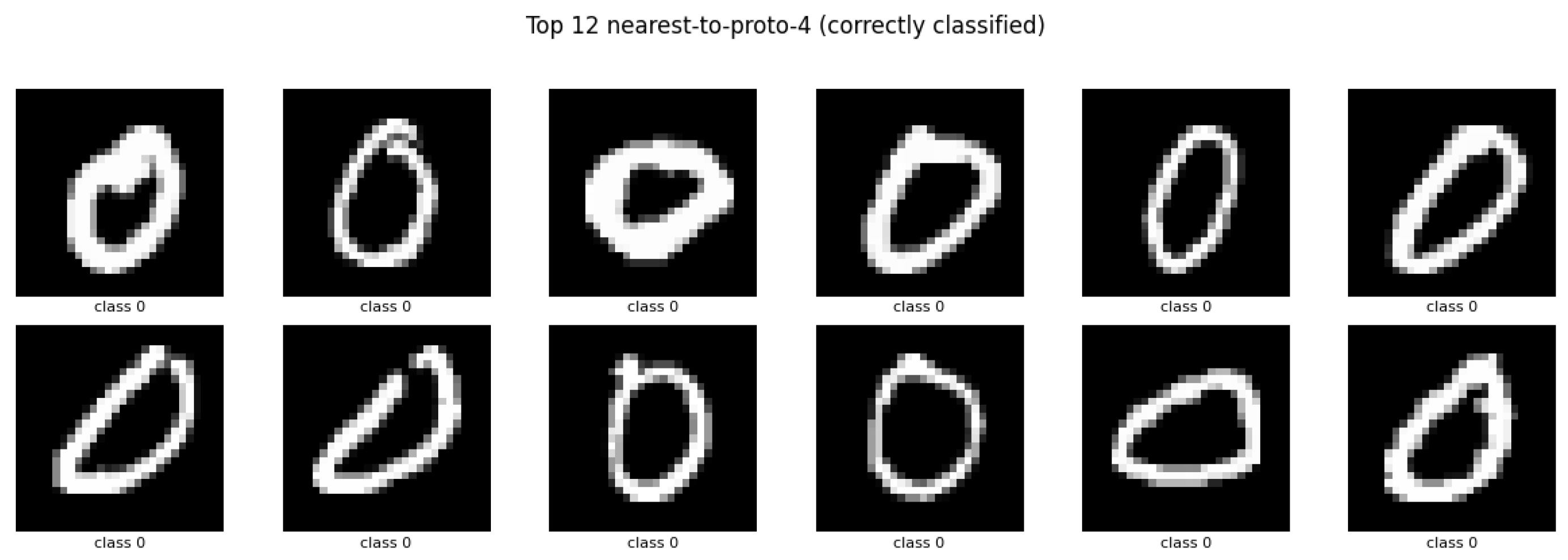
A detailed examination of the distilled model revealed an noteworthy behavior. Prototype #4, whose reconstruction clearly depicts a digit “0“ (see Figure 7), is associated by the weight matrix with the ”others” class with a probability of 66 %. An analysis of the twelve test images with latent encodings closest to this prototype (Figure 8) confirms that all correspond to well-formed instances of the digit “0”, each correctly classified as class “0“. Consequently, the prototype provides clear visual evidence of the digit “0” while functionally contributing to the decision for the opposing class. Because the mapping between prototypes and classes is learned independently of the visual characteristics of the prototypes, users lacking access to the weight matrix may be misled into believing that the model’s predictions for the “others” class are based on archetypal non-zero digits, when in fact the decisive signal is anchored in a visually canonical zero.
The binary classification setting thus amplifies a concern previously suggested by the multiclass experiments: prototype visualizations alone are insufficient to establish model trustworthiness. A prototype may function as a decoy, simultaneously presenting a compelling, human-interpretable exemplar while driving predictions for an unexpected class. Given that the distance vectors input to the linear classification head are high-dimensional, manual verification of class–prototype associations is impractical, and summary metrics such as normalized negative entropy (NNE) reflect only global sharpness rather than individual inconsistencies.
5. Conclusions
In this study, we introduced a novel prototype-based neural network architecture incorporating multiple prototype layers. We evaluated its performance and interpretability using the MNIST dataset, demonstrating both its representational capabilities and highlighting critical limitations concerning interpretability. Results demonstrate the network’s capacity to integrate and represent patterns across successive prototype layers. However, we observed a progressive decline in the visual interpretability of prototypes at deeper layers, complicating human understanding of the learned representations. Importantly, the decline in visual clarity at deeper prototype layers did not compromise the model’s predictive performance, which remained consistently high—indicating that the final prototype layer retained strong discriminative capacity despite reduced interpretability. A distilled shallow model, constructed by reusing the final prototype layer from the original deep prototype-based network (DPBN) as a fixed component, achieved a slight improvement in classification accuracy (99.83%). However, it exposed a critical flaw—prototypes visually representing “0” contributed internally to decisions for the “1” class. Hence, visualization of prototypes alone are insufficient for model transparency and reliable interpretability, and it is required to align visual and functional behaviors. Accordingly, we argue that prototype-based explanations within the “this-looks-like-that” paradigm necessitate additional safeguards—either through training constraints that enforce alignment between visual and functional semantics or via post-hoc auditing tools capable of identifying contradictory associations. A comprehensive investigation into such reliability guarantees is reserved for future work.
Author Contributions
Conceptualization, E.G-C.; methodology, E.G-C. and D.M.; software, R.I.; validation, E.G-C., D.M., and R.I.; formal analysis, E.G-C. and D.M.; investigation, E.G-C and R.I. and D.M.; data curation, R.I.; writing—original draft preparation, E.G-C. and R.I.; writing—review and editing, E.G-C and D.M.; visualization, R.I.; supervision, E.G-C.; All authors have read and agreed to the published version of the manuscript.
Funding
This research received no external funding.
Conflicts of Interest
The authors declare no conflicts of interest.
References
- Li, O.; Liu, H.; Chen, C.; Rudin, C. Deep Learning for Case-based Reasoning through Prototypes: A Neural Network that Explains its Predictions. CoRR 2017, abs/1710.04806, [1710.04806]. [Google Scholar] [CrossRef]
- Ras, G.; Xie, N.; Van Gerven, M.; Doran, D. Explainable deep learning: A field guide for the uninitiated. Journal of Artificial Intelligence Research 2022, 73, 329–396. [Google Scholar] [CrossRef]
- Deng, L. The mnist database of handwritten digit images for machine learning research. IEEE Signal Processing Magazine 2012, 29, 141–142. [Google Scholar] [CrossRef]
- Li, O.; Liu, H.; Chen, C.; Rudin, C. Deep Learning for Case-Based Reasoning through Prototypes: A Neural Network that Explains Its Predictions. In Proceedings of the Proceedings of the 32nd AAAI Conference on Artificial Intelligence, 2018.; ArXiv preprint arXiv:1710.04806 (v2, Nov. 2017).
- Chen, C.; Li, O.; Tao, D.; Barnett, A.; Rudin, C.; Su, J. This Looks Like That: Deep Learning for Interpretable Image Recognition. In Proceedings of the NeurIPS; 2019. [Google Scholar]
- Nauta, M.; van Bree, R.; Seifert, C. Neural Prototype Trees for Interpretable Fine-Grained Image Recognition. In Proceedings of the CVPR; 2021. [Google Scholar]
- Gulshad, S.; Long, T.; van Noord, N. Hierarchical Explanations for Video Action Recognition. In Proceedings of the 2023 IEEE/CVF Conference on Computer Vision and Pattern Recognition Workshops (CVPRW); 2023; pp. 3703–3708. [Google Scholar] [CrossRef]
- Koh, P.W.; Nguyen, T.; Tang, Y.S.; Mussmann, S.; Pierson, E.; Kim, B.; Liang, P. Concept Bottleneck Models. In Proceedings of the ICML; 2020. [Google Scholar]
- Papernot, N.; McDaniel, P. Deep k-Nearest Neighbors: Towards Confident, Interpretable and Robust Deep Learning. In Proceedings of the ICML; 2018. [Google Scholar]
- Sabour, S.; Frosst, N.; Hinton, G.E. Dynamic Routing Between Capsules. In Proceedings of the NeurIPS; 2017. [Google Scholar]
- Zhang, N.; Donahue, J.; Girshick, R.; Darrell, T. Part-based R-CNNs for Fine-grained Category Detection. In Proceedings of the ECCV; 2014. [Google Scholar]
- Bancroft, S. An Algebraic Solution of the GPS Equations. IEEE Transactions on Aerospace and Electronic Systems 1985, AES-21, 56–59. [Google Scholar] [CrossRef]
- Abel, J.; Chaffee, J. Existence and Uniqueness Analysis for the GPS Equations. IEEE Transactions on Aerospace and Electronic Systems 1991. [Google Scholar] [CrossRef]
- Norrdine, A. An Algebraic Solution to the Multilateration Problem. In Proceedings of the Proc. International Conference on Indoor Positioning and Indoor Navigation (IPIN); 2012; pp. 1–6. [Google Scholar]
- Levenberg, K. A Method for the Solution of Certain Non-Linear Problems in Least Squares. Quarterly of Applied Mathematics 1944, 2, 164–168. [Google Scholar] [CrossRef]
- Marquardt, D.W. An Algorithm for Least-Squares Estimation of Nonlinear Parameters. Journal of the Society for Industrial and Applied Mathematics 1963, 11, 431–441. [Google Scholar] [CrossRef]
- Moore, E.H. On the Reciprocal of the General Algebraic Matrix. Bulletin of the American Mathematical Society 1920, 26, 394–395. [Google Scholar]
- Penrose, R. A Generalized Inverse for Matrices. Proceedings of the Cambridge Philosophical Society 1955, 51, 406–413. [Google Scholar] [CrossRef]
- Bohle, M.; Singh, N.; Fritz, M.; Schiele, B. B-Cos Alignment for Inherently Interpretable CNNs and Vision Transformers. IEEE transactions on pattern analysis and machine intelligence 2024, PP. [Google Scholar] [CrossRef] [PubMed]
- Wolf, T.N.; Kavak, E.; Bongratz, F.; Wachinger, C. SIC: Similarity-Based Interpretable Image Classification with Neural Networks. 2025; arXiv:cs.CV/2501.17328. [Google Scholar]
- Turbé, H.; Bjelogrlic, M.; Mengaldo, G.; Lovis, C. ProtoS-ViT: Visual foundation models for sparse self-explainable classifications. 2024; arXiv:cs.CV/2406.10025. [Google Scholar]
- Singh, G.; Frizzo Stefenon, S.; Yow, K.C. The shallowest transparent and interpretable deep neural network for image recognition. Scientific Reports 2025, 15, 13940. [Google Scholar] [CrossRef] [PubMed]
- Leavitt, M.L.; Morcos, A. Selectivity considered harmful: evaluating the causal impact of class selectivity in DNNs. 2020; arXiv:cs.LG/2003.01262. [Google Scholar]
- Pearce, M.T.; Dooms, T.; Rigg, A.; Oramas, J.M.; Sharkey, L. Bilinear MLPs enable weight-based mechanistic interpretability. arXiv preprint arXiv:2410.08417 Analyzes bilinear MLP weight-spectrum for mechanistic interpretability. 2025, arXiv:2410.08417. [Google Scholar]
Figure 1.
DPBN architecture.
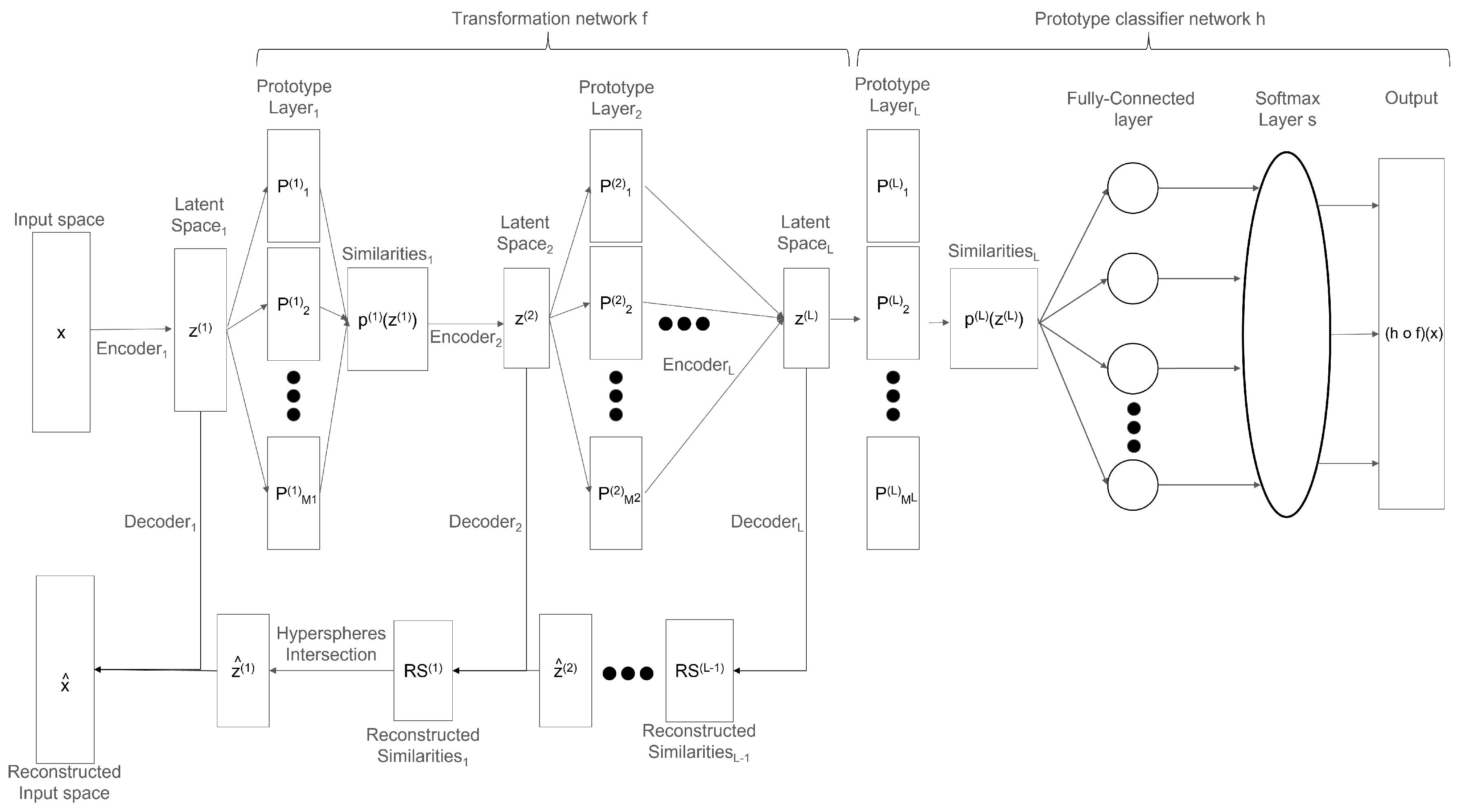
Figure 2.
Reconstructions of prototypes reveal that the uppermost panel (layer 1) exhibits digit-specific structures, while deeper layers (from top to bottom) tend to converge toward patterns that are less interpretable by humans due to their combination.
Figure 2.
Reconstructions of prototypes reveal that the uppermost panel (layer 1) exhibits digit-specific structures, while deeper layers (from top to bottom) tend to converge toward patterns that are less interpretable by humans due to their combination.
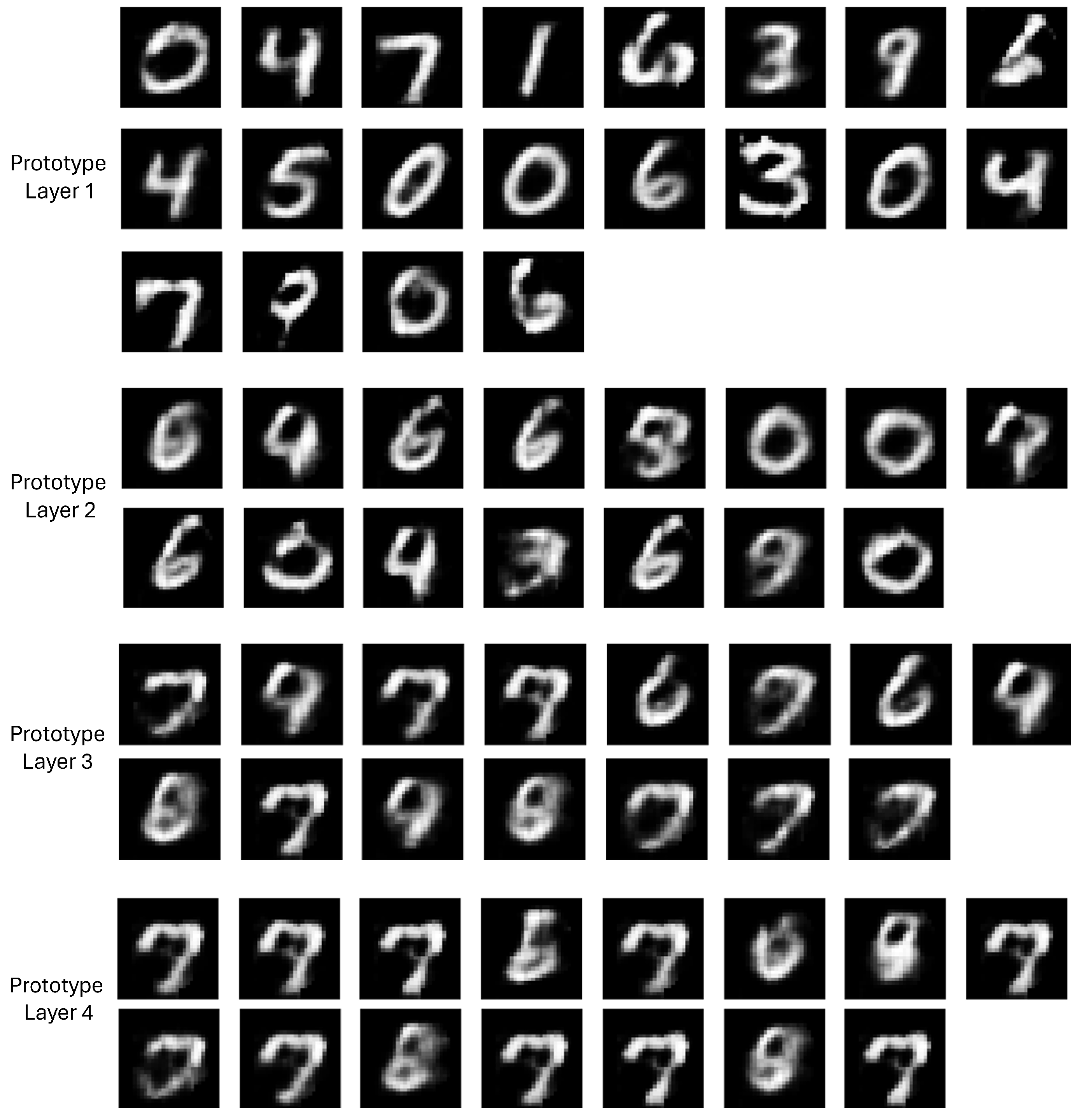
Figure 3.
Prototypes derived from the final layer in Experiment 2, presented alongside the corresponding weight matrix.
Figure 3.
Prototypes derived from the final layer in Experiment 2, presented alongside the corresponding weight matrix.
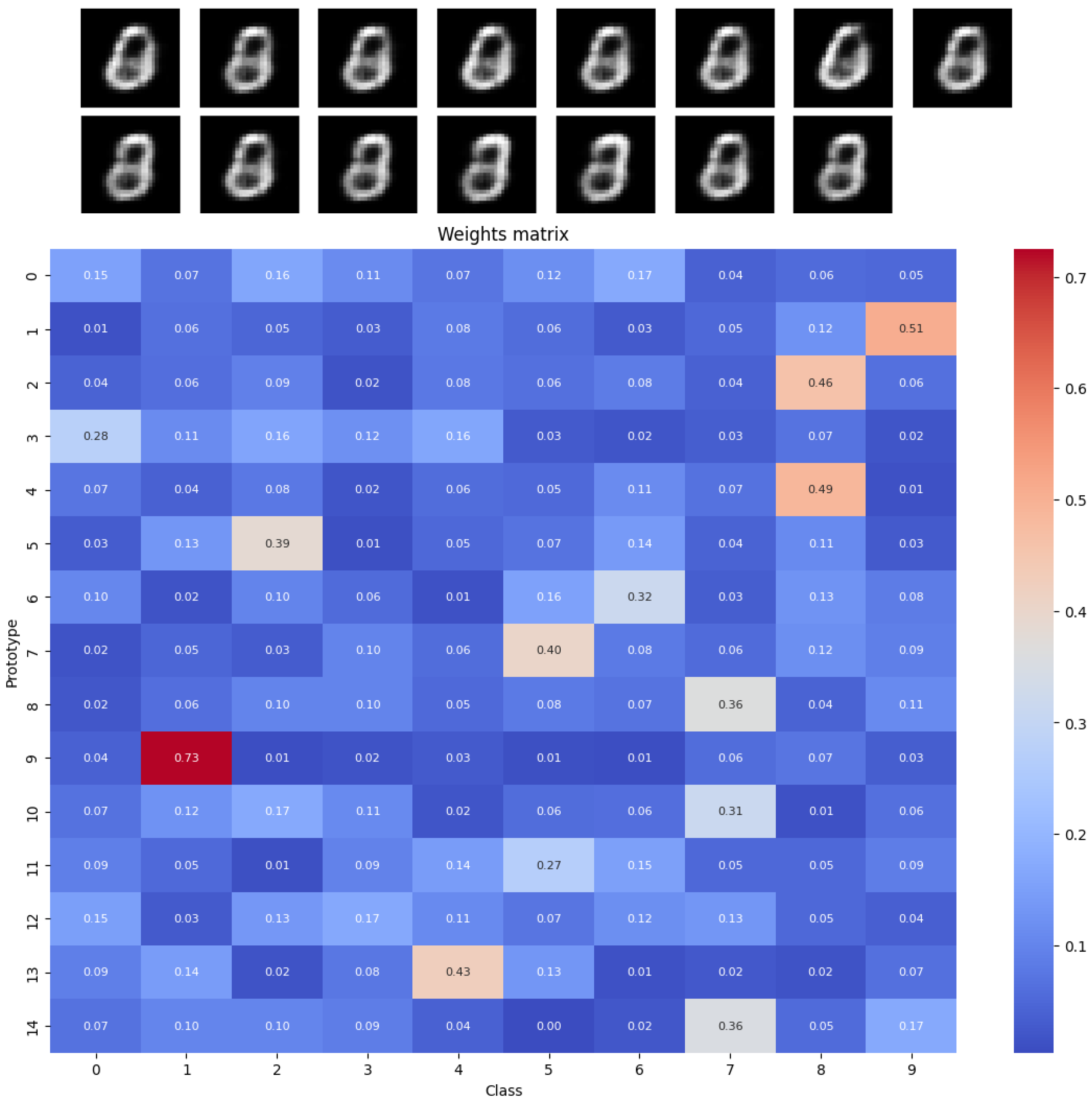
Figure 4.
Prototypes obtained from those transferred from a 4-layer Deep Prototype-Based Network (DPBN) in Experiment 2, shown together with the corresponding weight matrix.
Figure 4.
Prototypes obtained from those transferred from a 4-layer Deep Prototype-Based Network (DPBN) in Experiment 2, shown together with the corresponding weight matrix.
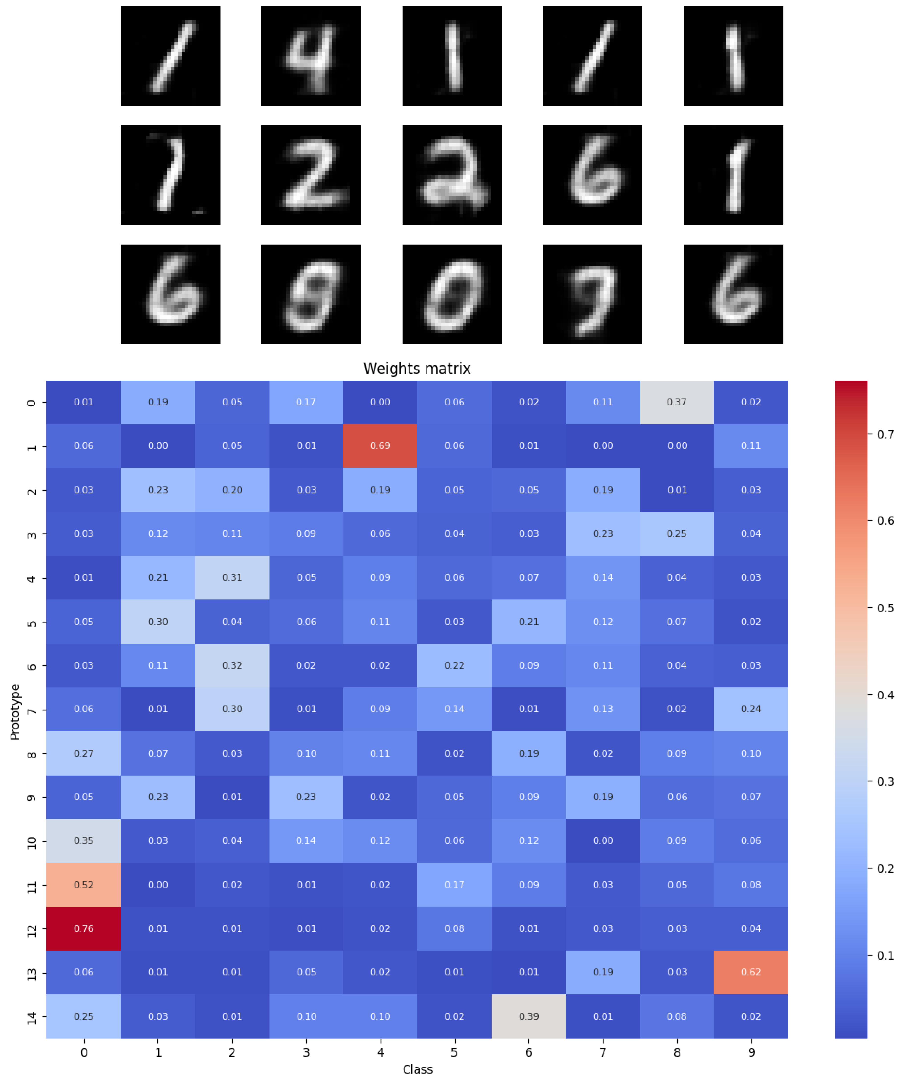
Figure 5.
Reconstructed prototypes from the last layer showing a low degree of interpretability.
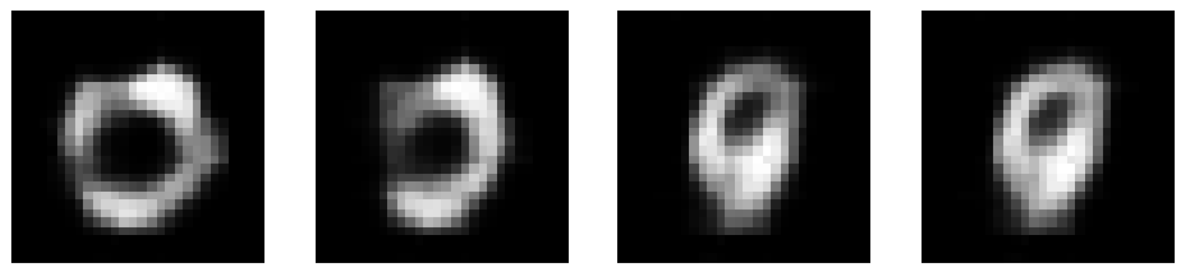
Figure 6.
Softmax-normalised weight matrix of the deep prototype network. Rows correspond to prototypes, columns to the two classes. Prototype #4 (bottom row) is visually a digit “0’’ yet assigns the bulk of its weight to the other class.
Figure 6.
Softmax-normalised weight matrix of the deep prototype network. Rows correspond to prototypes, columns to the two classes. Prototype #4 (bottom row) is visually a digit “0’’ yet assigns the bulk of its weight to the other class.
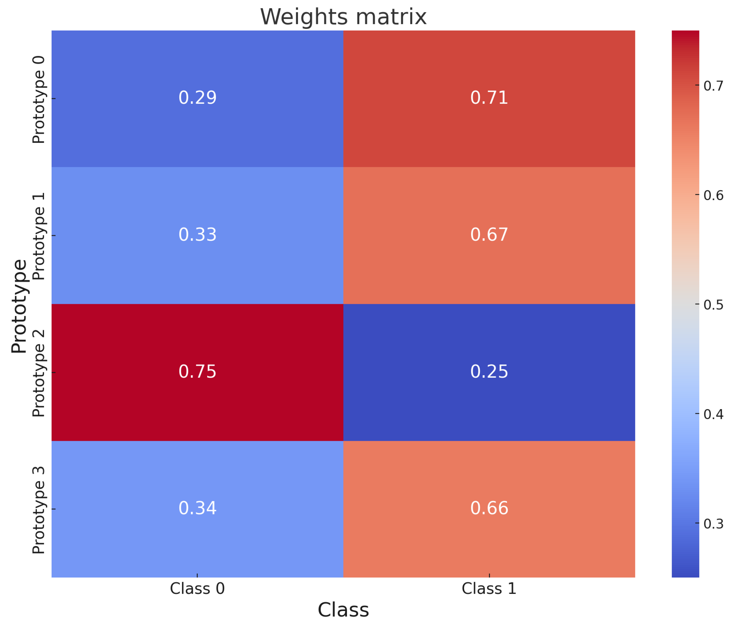
Figure 7.
Reconstructed deepest-layer prototypes after training. The last prototype (right-most) is a clear “0’’ despite its functional association with the other class.
Figure 7.
Reconstructed deepest-layer prototypes after training. The last prototype (right-most) is a clear “0’’ despite its functional association with the other class.
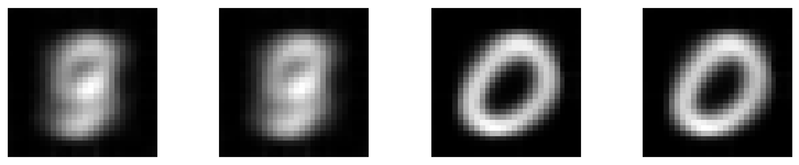
Figure 8.
Twelve test images nearest to Prototype #4 in latent space, all correctly labelled as class “0’’.
Figure 8.
Twelve test images nearest to Prototype #4 in latent space, all correctly labelled as class “0’’.
Disclaimer/Publisher’s Note: The statements, opinions and data contained in all publications are solely those of the individual author(s) and contributor(s) and not of MDPI and/or the editor(s). MDPI and/or the editor(s) disclaim responsibility for any injury to people or property resulting from any ideas, methods, instructions or products referred to in the content. |
© 2025 by the authors. Licensee MDPI, Basel, Switzerland. This article is an open access article distributed under the terms and conditions of the Creative Commons Attribution (CC BY) license (http://creativecommons.org/licenses/by/4.0/).
Copyright: This open access article is published under a Creative Commons CC BY 4.0 license, which permit the free download, distribution, and reuse, provided that the author and preprint are cited in any reuse.