
Submitted:
22 July 2025
Posted:
23 July 2025
You are already at the latest version
Abstract
The Economic Dispatch Problem (EDP) plays a critical role in power system operations by trying to allocate power generation across multiple units at minimal cost while satisfying complex operational constraints. Traditional optimization techniques struggle with the non-convexities introduced by factors such as valve-point effects, prohibited operating zones, and spinning reserve requirements. While metaheuristics methods have shown promise, they often suffer from convergence issues and constraint-handling limitations. In this study, we introduce a novel application of Group Relative Policy Optimization (GRPO), a reinforcement learning framework that extends Proximal Policy Optimization by integrating group-based learning and relative performance assessments. The proposed GRPO approach incorporates smart initialization, adaptive exploration, and elite-guided updates tailored to the EDP’s structure. Our method consistently produces high-quality, feasible solutions with faster convergence compared to state-of-the-art metaheuristics and learning-based methods. For instance, in the case of the 15-unit system, GRPO achieved a best cost of $32421.67/h with full constraint satisfaction in just 4.24 seconds, surpassing many previous solutions. The algorithm also demonstrates excellent scalability, generalizability, and stability across larger-scale systems without requiring parameter retuning. These results highlight GRPO’s potential as a robust and efficient tool for real-time energy scheduling in smart grid environments.
Keywords:
economic dispatch problem
; reinforcement learning
; group relative policy optimization
; smart grid
; nonconvex optimization
; constraint handling
; energy scheduling
1. Introduction
The rapid evolution of electrical grids toward smart grid architectures has fundamentally transformed the landscape of power systems operation and control. Smart grids integrate advanced sensing, communication, and computing technologies with traditional power infrastructure to enhance efficiency, reliability, and sustainability [1]. This modernization enables real-time monitoring, bidirectional communication, and dynamic adaptation to changing conditions, thereby facilitating the integration of renewable energy sources, demand response mechanisms, and distributed generation [2]. However, these advancements also introduce significant complexity into the optimal management of power generation resources, making the Economic Dispatch Problem (EDP) increasingly challenging yet critical for efficient grid operation.
The Economic Dispatch Problem represents a fundamental optimization challenge in power systems engineering, focusing on determining the optimal power output allocation among available generating units to meet the system demand while minimizing total operating costs [3]. In the context of smart grids, the EDP must additionally account for the intermittency of renewable resources, demand-side flexibility, energy storage systems, and various operational constraints such as prohibited operating zones, valve-point effects, and ramp rate limits [4,5]. The efficient solution of the EDP is paramount as even marginal improvements in cost efficiency can translate to substantial economic savings given the scale of modern power systems.
Traditional approaches to solving the EDP have relied on classical mathematical optimization techniques, including linear programming, quadratic programming, lambda iteration, and gradient methods [3]. While these methods provide exact solutions for convex and well-behaved problems, they face significant limitations when confronted with real-world EDP instances characterized by non-convexity, discontinuities, and multiple local optima. The incorporation of realistic constraints such as prohibited operating zones and valve-point effects renders the problem highly non-linear and non-convex, causing classical methods to struggle with convergence or become trapped in suboptimal solutions [6].
To overcome these limitations, metaheuristic optimization algorithms have emerged as viable alternatives for tackling complex EDP instances. Techniques such as Genetic Algorithms (GA), Particle Swarm Optimization (PSO), Differential Evolution (DE), Grey Wolf Optimizer (GOP) and Artificial Bee Colony (ABC) have demonstrated considerable success in navigating the complex search spaces of modern EDP formulations [7,8]. These population-based approaches offer the advantages of global exploration capability, constraint-handling flexibility, and reduced sensitivity to initial conditions. However, metaheuristics also exhibit notable limitations, including parameter sensitivity, convergence inconsistency, and the absence of theoretical guarantees regarding solution quality. Moreover, their performance often deteriorates when scaling to high-dimensional problems or when addressing dynamic environments where system conditions evolve rapidly [9].
The limitations of metaheuristics have motivated the exploration of Reinforcement Learning (RL) approaches for economic dispatch optimization. RL methods offer several distinctive advantages, including the ability to learn optimal policies through interaction with the environment, adaptation to changing conditions, and incorporation of sequential decision-making frameworks that align well with power system operations [10]. Nevertheless, classical RL methods such as Q-learning and Deep Q-Networks (DQN) face challenges related to sample efficiency, exploration-exploitation balance, and high-dimensional continuous action spaces that are characteristic of the EDP.
Group Relative Policy Optimization (GRPO) addresses these challenges by extending the traditional Proximal Policy Optimization (PPO) framework to incorporate collective learning dynamics and relative policy improvements. Unlike conventional RL methods that update policies based solely on absolute performance metrics, GRPO leverages information sharing and relative performance assessments within groups of agents to enhance convergence stability and exploration efficiency [11]. By establishing trust regions based on the relative performance of multiple solution candidates, GRPO mitigates the risks of premature convergence and policy degradation during training. Additionally, the group-based approach enables more effective constraint handling through collaborative learning, where feasible solutions inform the development of effective constraint satisfaction strategies across the entire population of agents.
In this work, we present a novel application of GRPO for solving complex Economic Dispatch Problems in smart grid environments. The main contributions of this research are threefold: (1) the development of a specialized GRPO framework tailored to the unique characteristics of the EDP, incorporating domain-specific knowledge into the policy and value network architectures; (2) an enhanced constraint-handling mechanism that preserves solution feasibility through adaptive penalty formulations and guided exploration of the feasible region; and (3) comprehensive empirical evaluation demonstrating superior performance compared to both traditional metaheuristics and conventional RL approaches across a diverse set of benchmark problems and real-world case studies.
The remainder of this paper is organized as follows: Section 2 presents a formal mathematical formulation of the Economic Dispatch Problem, including the objective function and various operational constraints considered in this study. Section 3 provides a comprehensive review of related work spanning classical methods, metaheuristics, and reinforcement learning approaches for economic dispatch. Section 4 introduces the proposed GRPO methodology, detailing the algorithm design, network architectures, and constraint-handling mechanisms. Section 5 describes the experimental setup, including benchmark problems, comparison methods, and evaluation metrics. Section 6 presents and discusses the experimental results, highlighting the performance advantages of GRPO across different problem instances. Finally, Section 7 concludes the paper with a summary of findings, limitations, and directions for future research.
2. Related Work
Economic Dispatch (ED) is a fundamental optimization problem in power systems, where the goal is to allocate generation among available units to meet a certain load at minimum cost. In multi-objective formulations of ED, additional objectives such as emission minimization or loss reduction are considered alongside cost, making the problem a multi-criteria optimization challenge. The ED problem is subject to numerous constraints, including power balance, generator output limits, ramp rate limits, and sometimes more complex operational constraints like prohibited operating zones or multi-area power transfer limits [12]. Solving ED optimally is crucial for both economic efficiency and environmental compliance in modern grids. Over the past decade, there has been significant progress in solution methods for ED, especially for non-convex and multi-objective versions. These methods span classical mathematical optimization, metaheuristic algorithms, and machine learning, including reinforcement learning approaches, each with its own merits and limitations. In this section, we explore and discusses each category in turn, with an emphasis on the state-of-the-art metaheuristic and learning-based techniques for multi-objective ED, and highlights the challenges associated with them to motivate our approach.
2.1. Classical Mathematical Approaches
Classical methods for ED rely on mathematical programming and optimization theory. For the basic ED with a single objective (e.g., fuel cost minimization) and convex cost curves, the problem can be formulated as a convex optimization (e.g., a quadratic program) and solved to global optimality using efficient algorithms [13]. Lambda-iteration (gradient method) and Lagrange relaxation have been long-standing techniques: the lambda-iteration method equalizes the incremental cost () across units to satisfy optimality and balance conditions, and it works well when generator cost functions are smooth and convex. In fact, early implementations of ED in the 1960s applied linear programming techniques to economic generation allocation [12]. Later methods like dynamic programming were used for unit commitment and dispatch problems in the 1960s–70s. Quadratic programming methods (e.g., using the Kuhn–Tucker conditions) and network flow approaches which treat ED as a transportation problem were also explored in the literature [13]. However, classical optimization methods encounter limitations as the ED problem becomes more realistic. One major issue is non-convexity. Practical ED often involves valve-point effect ripples in cost functions, multiple fuel options for generators, or prohibited operating zones, all of which introduce non-smooth, non-convex characteristics [13,14,15]. Traditional solvers such as LP or QP struggle with these; they might converge to a local optimum or require piecewise-linear approximations to fit into a convex model [13]. For instance, including emission cost as a second objective or constraint was handled in the 1990s by techniques like Lagrangian relaxation [16], but those methods needed convexified formulations. Classic methods also have difficulty with discrete decision variables like unit on/off states or integer transmission flow limits without resorting to combinatorial search techniques that exponentially increase complexity. While methods like dynamic programming and branch-and-bound can handle discrete unit commitment, they suffer from the curse of dimensionality for large-scale systems [16]. Another limitation is in handling multiple objectives. Classical approaches typically scalarize multiple objectives (e.g., combine cost and emission into a single weighted sum objective). This requires choosing weighting factors a priori, which can be arbitrary and may not capture the true trade-offs. There is no straightforward way for classical deterministic solvers to produce a Pareto-optimal set of solutions in one run – they would need to be run multiple times with different weights or targets. This lack of flexibility is a drawback in multi-objective ED scenarios [16]. Finally, computational scalability is a concern: although methods like the lambda-iteration are extremely fast for convex ED and were historically used in real-time dispatch computers, they cannot guarantee optimality for non-convex ED [13]. Techniques like quadratic programming or nonlinear programming can solve moderately sized problems, but their performance degrades as the number of generators and constraints grows. In summary, while classical mathematical methods form the foundation and can solve simplified ED efficiently, they struggle with the complex, non-convex, and multi-objective nature of modern ED problems. These limitations motivated the development of metaheuristic methods that can more easily handle such complexities.
2.2. Metaheuristic Approaches
Metaheuristic algorithms have emerged as key methods for economic dispatch (ED), especially in non-convex and multi-objective scenarios, due to their ability to handle complex, nonlinear constraints without strict assumptions on objective functions [14,15]. Although these algorithms do not guarantee global optima, they typically yield high-quality solutions efficiently. Genetic Algorithms (GA), among the earliest used for ED, utilize evolutionary processes including crossover and mutation. GAs effectively manage valve-point effects and multi-fuel scenarios [17], with multi-objective variants like NSGA-II frequently generating Pareto fronts for economic-emission trade-offs. However, GAs may suffer from slow convergence and require careful parameter tuning. Constraint handling commonly involves penalty functions or repair operators to ensure feasibility [12]. Particle Swarm Optimization (PSO) which is inspired by flocking behavior offers simpler implementation and faster convergence than GAs, as evidenced in seminal work by [18]. PSO effectively addresses high-dimensional search spaces due to rapid information sharing and minimal parameter tuning. Multi-objective PSO (MOPSO) manages environmental/economic dispatch by maintaining solution diversity. PSO’s simplicity enables near real-time application, though occasional stagnation and parameter sensitivity remain concerns [19].
Differential Evolution (DE) uses vector differences and recombination to achieve efficient continuous optimization [20]. DE often outperforms GA and PSO on complex ED problems, particularly when hybridized or adapted through specialized mechanisms, such as single-unit adjustment repairs for constraint violations [12]. Adaptive strategies enhance DE’s robustness, especially in multi-objective contexts, though parameter choice and discrete handling limitations persist. Ant Colony Optimization (ACO), although traditionally for combinatorial optimization, is applied to discrete or hybrid ED problems. It generally performs less efficiently than GA, PSO, or DE for purely continuous ED but can excel in hybrid scenarios involving unit commitment or discrete decisions. Multi-objective ACO adaptations exist but require substantial computational resources and careful tuning [7]. Recent metaheuristics like the Grey Wolf Optimizer (GWO) have gained attention due to their simplicity and balanced exploration-exploitation capabilities, showing competitive results on complex ED scenarios [7]. Numerous other novel algorithms, including Whale Optimization, Bat, and Firefly, have demonstrated effectiveness in ED, especially when hybridized or parameter-adaptive. These methods typically handle constraints via penalties, repairs, or dependent variable encoding, achieving near-real-time performance with optimization strategies like parallelization and warm starts.
Overall, metaheuristics significantly extend the solvability of ED problems beyond classical methods, addressing multi-modal and multi-objective challenges effectively. Despite their inherent lack of optimality guarantees and sensitivity to parameterization, these methods remain central to ED research and practice, increasingly augmented by emerging reinforcement learning-based approaches.
2.3. Machine Learning and Reinforcement Learning Approaches
Machine Learning (ML) techniques have recently emerged as promising alternatives to conventional optimization methods for solving Economic Dispatch problems, encompassing supervised learning, hybrid methods, and particularly Reinforcement Learning (RL). Supervised ML approaches utilize historical real data or data generated by offline optimizers (e.g., linear programming or metaheuristics) to train predictive models like Decision Trees or Neural Networks, providing fast dispatch decisions in real-time scenarios. For instance, Goni et al. [21] employed a Decision Tree trained on data from the Lagrange multiplier method, significantly reducing computation time compared to classical solvers. However, such methods depend heavily on comprehensive, stationary training datasets and require retraining upon system alterations. Additionally, hybrid strategies involving ML-guided metaheuristics have been explored; notably, Visutarrom et al. [22] used RL to adaptively tune Differential Evolution parameters, enhancing robustness and reducing manual tuning efforts.
Building upon these approaches, Reinforcement Learning methods have become particularly prominent, offering advantages for dynamic ED scenarios involving uncertainty and sequential decision-making. RL methods learn dispatch policies mapping system states (loads, generation statuses) directly to optimal generator actions, utilizing algorithms such as Q-learning, Deep Q-Networks (DQN), Deep Deterministic Policy Gradient (DDPG), and Proximal Policy Optimization (PPO). While classical Q-learning faces limitations due to discrete state-action spaces, DQN employs neural network approximations to effectively handle larger continuous state spaces. [23] highlighted DQN’s superior performance in battery dispatch scenarios, demonstrating significant cost savings through optimal charge/discharge policies.
Addressing continuous action spaces essential for ED, policy gradient methods like DDPG and PPO have shown significant promise. [24] successfully applied hybrid DDPG for microgrid dispatch, achieving superior performance compared to discretized DQN. PPO has been favored for its stability during training, with studies demonstrating its efficacy in learning robust dispatch policies in renewable-integrated dynamic ED contexts.
Expanding on these methods, advanced RL techniques such as Soft Actor-Critic (SAC) and emerging Group Relative Policy Optimization (GRPO) have shown potential for overcoming inherent RL limitations like training complexity and critic network biases. While SAC’s stochastic nature has proved less effective for deterministic dispatch scenarios, GRPO’s critic-free design promises enhanced training efficiency, although its practical application in ED remains exploratory.
To successfully implement RL methods, careful consideration must be given to designing states, actions, and rewards. Incorporating temporal indicators significantly enhances policy adaptability [23]. Continuous dispatch adjustments typically favor actor-critic methods, whereas discrete action spaces are suitable for DQN. Furthermore, multi-agent RL presents a potential avenue for managing large-scale dispatch tasks, although ensuring cooperative behavior among multiple agents adds complexity. Reward functions typically integrate economic objectives with penalties for constraint violations. However, excessive emphasis on penalties can hinder cost optimization. Thus, hard-coding domain-specific constraints often supplements reward shaping, guiding RL agents primarily towards minimizing economic costs. Despite these advancements, trained RL policies face several challenges. Although execution is rapid and suitable for real-time deployment, RL training itself is computationally intensive and time-consuming. Moreover, RL-derived policies do not guarantee global optimality and exhibit limited generalization beyond training scenarios, necessitating continuous retraining. Policy explainability and safe exploration also remain significant issues, particularly for operational grid deployments. Nevertheless, RL’s adaptability and real-time responsiveness provide substantial benefits in evolving smart-grid applications. Hybrid frameworks combining RL-derived dispatch policies with deterministic refinement processes could ensure feasibility and operational reliability, effectively bridging learning-based methods and traditional optimization techniques.
3. Problem Formulation
This section presents a comprehensive mathematical formulation of the Economic Dispatch Problem (EDP), providing the necessary foundation for understanding the optimization challenges addressed in this work. We begin with the basic convex formulation before examining the more complex nonconvex variants that incorporate realistic operational constraints.
3.1. Convex Economic Dispatch Problem
The fundamental objective of the Economic Dispatch Problem is to minimize the total production cost while satisfying various system constraints. The objective function can be mathematically expressed as:
where represents the total generation cost, is the cost function of the i-th generating unit, is the power output of the i-th generating unit, and N is the total number of generating units in the system.
In its most basic form, the fuel cost of a thermal generation unit is typically represented as a quadratic function:
where , , and are the cost coefficients of the i-th generating unit. However, to more accurately model the actual response of thermal generators, higher-order polynomial functions may be employed. A cubic cost function, for instance, provides enhanced modeling precision and can be represented as:
where is the cubic cost coefficient of the i-th generating unit.
The optimization is subject to several operational constraints that must be satisfied for a feasible solution:
3.1.1. Power Balance Constraint
The total power generated must equal the total demand plus transmission losses:
where represents the total system demand and denotes the transmission losses. The transmission losses can be calculated using Kron’s loss formula, also known as the B-matrix coefficient method:
where , , and are the loss coefficients or B-coefficients.
3.1.2. Generator Capacity Constraints
The power output of each generating unit must remain within its operational limits:
where and are the minimum and maximum power outputs of the i-th generating unit, respectively.
3.2. Nonconvex Economic Dispatch Problems
Real-world power systems often exhibit nonconvex characteristics due to various physical and operational constraints. We consider two significant sources of nonconvexity in the EDP: valve-point effects and prohibited operating zones.
3.2.1. Valve-Point Effects
In thermal power plants, each steam admission valve in a turbine produces a rippling effect on the unit’s heat rate curve when it begins to open. This phenomenon, known as the valve-point effect (VPE), introduces significant nonlinearities in the cost function, resulting in multiple local optima. The cost function incorporating valve-point effects can be modeled as:
where and are the valve-point effect coefficients. The sinusoidal term introduces ripples in the cost function, making the optimization landscape significantly more complex, as illustrated in Figure 1.
3.2.2. Prohibited Operating Zones
Prohibited operating zones (POZ) are specific ranges of power output where the operation of generating units is restricted due to physical limitations such as vibrations in the shaft bearings, resonance in certain components, or other mechanical constraints. Operating within these zones could potentially damage equipment or cause instability in the system. The presence of prohibited operating zones introduces discontinuities in the feasible region, further complicating the optimization process.
For units with prohibited operating zones, the feasible operating regions can be mathematically defined as:
where and represent the lower and upper bounds of the k-th prohibited zone of the i-th unit, respectively, and is the number of prohibited zones for the i-th generating unit.
3.3. Additional Operational Constraints
Modern power systems often incorporate additional constraints that must be satisfied for secure and reliable operation:
3.3.1. Spinning Reserve Constraint
Spinning reserve represents the extra generating capacity that is available by increasing the power output of generators already connected to the power system. This constraint ensures that sufficient reserve capacity is available to respond to unforeseen load increases or generation outages:
where is the spinning reserve contribution of the i-th generating unit and is the total spinning reserve requirement. The spinning reserve contribution of each unit is determined by:
where is the maximum spinning reserve capability of the i-th unit and is the set of units that cannot provide spinning reserve.
3.3.2. Ramp Rate Constraints
The ramp rate constraints limit the rate at which the power output of a generating unit can change between consecutive time periods, reflecting the physical limitations of thermal units:
where is the previous power output of the i-th unit, and and are the ramp-up and ramp-down rate limits, respectively. To incorporate these constraints into the generator capacity limits, Equation (6) can be reformulated as:
3.4. Constraint Handling Approaches
Effectively managing constraints is crucial for solving the EDP. In this work, we employ several techniques to handle different types of constraints:
3.4.1. Slack Variable Method for Equality Constraints
For the power balance constraint, we adopt a slack variable approach where one unit (typically referred to as the slack unit) is designated to compensate for any imbalance. The power output of the slack unit is calculated as:
where is the power output of the slack unit, which is randomly selected from the available units. If the calculated value of violates its limits, a penalty is applied to the objective function.
3.4.2. Penalty Function Approach for Inequality Constraints
For inequality constraints such as generator limits, prohibited operating zones, and spinning reserve requirements, we employ a penalty function approach where violations are penalized in the objective function:
where is the penalized objective function, C is the set of all constraints, is the penalty coefficient for constraint c, and is the magnitude of the violation of constraint c.
4. Group Relative Policy Optimization
Group Relative Policy Optimization (GRPO) represents an innovative approach in reinforcement learning that extends traditional policy optimization methods through the incorporation of group dynamics and relative performance assessments. This section presents both a conceptual overview and the mathematical formulation of the GRPO methodology.
4.1. Core Principles
GRPO is fundamentally built on three key principles:
- Group-based Learning: Instead of training a single policy, GRPO maintains a population of policies that learn collaboratively.
- Relative Performance Assessment: Policies are evaluated not only on their absolute performance but also on their performance relative to other policies in the group.
- Trust Region Optimization: Policy updates are constrained to prevent excessive deviations from the established consensus of the group.
4.2. The GRPO Framework
The GRPO framework can be understood as an organized approach consisting of the following components:
4.2.1. Policy Population
GRPO maintains a diverse population of policies, typically ranging from 10 to 50 depending on the complexity of the problem. Each policy represents a potential solution strategy and is characterized by its own set of parameters. The population-based approach provides several advantages:
- Multiple starting points in the solution space, reducing the risk of being trapped in local optima
- Diverse exploration strategies that collectively cover more of the solution space
- Robustness against individual policy failures through information sharing
4.2.2. Relative Advantage Estimation
A cornerstone of GRPO is its novel approach to advantage estimation. In standard reinforcement learning, the advantage function measures how much better an action is compared to the average action in a given state. GRPO extends this concept by computing a relative advantage that compares the performance of a policy not just against itself but against the entire policy group.
4.2.3. Elite Reference Set
After each evaluation phase, GRPO identifies an elite subset of policies that demonstrated superior performance. This elite set serves multiple purposes:
- Providing reference strategies for other policies to learn from
- Stabilizing the learning process by preserving successful approaches
- Guiding the exploration toward promising regions of the solution space
4.2.4. Group Trust Region
To ensure stable learning progress, GRPO implements a group-based trust region mechanism. This approach constrains policy updates to prevent any single policy from deviating too far from the group consensus. The group trust region offers several benefits:
- Improved stability during learning
- Prevention of catastrophic forgetting
- Balanced exploration and exploitation across the policy population
4.3. Learning Process
The GRPO learning process follows a cyclical pattern consisting of four main phases:
- Experience Collection: Each policy interacts with the environment independently
- Relative Performance Evaluation: Policies are assessed against the group
- Elite Selection: Top-performing policies are identified (typically 20-30%)
- Policy Update: All policies are updated based on their experience and elite influence
4.4. Mathematical Formulation
4.4.1. Policy Parameterization
In GRPO, we maintain a population of K policies, each parameterized by , where . The stochastic policy defines a probability distribution over actions given a state . For continuous action spaces, the policy is typically modeled as a multivariate normal distribution:
where represents the mean action and is the covariance matrix, both functions of the current state and parameterized by .
4.4.2. Relative Advantage Function
For each policy , we define the relative advantage function:
where is the standard advantage function for policy , calculated as:
The relative advantage function quantifies how much better (or worse) an action is compared to the average performance of the policy group. This provides a more informative learning signal that accounts for the collective exploration of the state-action space.
4.4.3. Objective Function
The GRPO objective function for policy combines the standard PPO clipped objective with a relative performance term:
where is the importance sampling ratio, is the clipping parameter (typically 0.1 or 0.2), and is a hyperparameter controlling the influence of the relative performance term. The relative importance sampling ratio is defined as:
4.4.4. Group-Based Trust Region
GRPO employs a group-based trust region mechanism to ensure stable policy updates. This is implemented through a novel group Kullback-Leibler (KL) divergence constraint:
where is the maximum allowable divergence. The group KL divergence is computed as:
This constraint prevents any single policy from deviating too far from the group consensus, promoting stability while still allowing for exploration.
4.4.5. Elite Selection and Update
After evaluating all policies in the group, GRPO employs an elite selection mechanism to identify the most promising candidates:
where is the performance of policy and is typically set to select the top (e.g., ) of policies. The elite policies influence the update of the entire population through a soft update mechanism:
where is a policy-specific update coefficient that controls the balance between individual learning and group influence.
4.5. Adaptive Hyperparameter Tuning
GRPO incorporates adaptive mechanisms to tune critical hyperparameters throughout the learning process:
4.5.1. Adaptive Learning Rate
The learning rate for each policy is adjusted based on the policy’s relative performance:
where is the base learning rate, is the average performance across all policies, is the standard deviation of performances, and is a scaling factor.
4.5.2. Adaptive Exploration
The exploration rate, which controls the covariance matrix , is adapted based on the diversity of the policy group:
where is the base exploration rate and is a scaling factor. This mechanism increases exploration when the policy is significantly different from others, promoting effective coverage of the search space.
4.6. Theoretical Properties
GRPO possesses several notable theoretical properties that distinguish it from traditional policy optimization methods:
4.6.1. Improved Sample Efficiency
By leveraging information from multiple policies, GRPO makes more efficient use of collected samples. Each trajectory contributes to the update of multiple policies through the relative advantage mechanism, effectively increasing the effective sample size without additional environment interactions.
4.6.2. Enhanced Exploration
The group-based approach naturally encourages diversity among policies, as each policy receives different update signals based on its relative performance. This implicit exploration mechanism helps avoid premature convergence to suboptimal solutions.
4.6.3. Stronger Convergence Guarantees
Under certain conditions, GRPO can be shown to converge to at least a local optimum with higher probability than single-policy methods. The group dynamics provide robustness against individual policy failures and help escape local optima through the sharing of information across the population.
4.6.4. Performance Bounds
The performance of the GRPO algorithm can be bounded as follows:
where is the policy learned by GRPO, is a baseline policy, is the discount factor, and is the state distribution under the baseline policy.
4.7. Key Advantages of GRPO
GRPO offers several significant advantages over traditional policy optimization methods:
4.7.1. Enhanced Exploration
The population-based approach naturally encourages diverse exploration strategies. Different policies can specialize in different regions of the state-action space, collectively providing more comprehensive coverage than a single policy could achieve. Furthermore, the relative performance assessment rewards policies that discover novel effective strategies, explicitly promoting exploration.
4.7.2. Improved Stability
The group trust region mechanism prevents policies from making drastic updates that could destabilize the learning process. By constraining updates relative to the group consensus, GRPO maintains a more stable learning trajectory even in highly complex or noisy environments.
4.7.3. Robustness to Local Optima
Traditional reinforcement learning methods often struggle with local optima, especially in non-convex optimization landscapes. GRPO’s multi-policy approach provides multiple entry points into the solution space, significantly reducing the risk of all policies becoming trapped in the same suboptimal solution.
4.7.4. Efficient Knowledge Sharing
Through the elite reference set and relative advantage computation, GRPO enables efficient sharing of knowledge across the policy population. Successful strategies discovered by one policy can quickly propagate to others, accelerating the overall learning process without requiring explicit communication protocols.
5. GRPO Implementation for Economic Dispatch Problem
This section presents the implementation of Group Relative Policy Optimization (GRPO) for solving the Economic Dispatch Problem (EDP). We describe the specialized adaptations and design choices made to effectively apply GRPO to the complex constraints and nonlinearities characteristic of modern EDP instances.
5.1. Problem Representation
To effectively apply GRPO to the Economic Dispatch Problem, we must first establish an appropriate problem representation that aligns with the reinforcement learning framework.
5.1.1. State and Action Spaces
For the EDP, the state space consists of relevant system parameters:
- Power demand ()
- Current generator outputs
- System constraints including prohibited operating zones
- Spinning reserve requirements
The action space represents the power output allocations for all generators. Given that the EDP involves continuous values within specific ranges, we normalize the action space to where N is the number of generators. Each normalized action is then mapped to the actual power output using:
where is the normalized action for generator i, and is the corresponding power output.
5.2. GRPO Architecture for EDP
5.2.1. Policy Population Design
Based on the provided code, our GRPO implementation maintains a population of policies represented by a collection of potential generator power allocations. The SimplifiedPPOOptimizer class implements this population-based approach with the following parameters:
Each member of the population represents a candidate solution to the EDP, encoded as a vector of normalized power outputs across all generators.
5.2.2. Smart Initialization Strategy
Rather than random initialization, our implementation employs a smart initialization strategy that allocates power proportionally based on generator efficiency:
where is the quadratic cost coefficient of generator i and is a small constant to prevent division by zero. Initial power allocations are then calculated as:
This initialization approach ensures that the GRPO algorithm begins with reasonable solutions that prioritize more efficient generators while respecting operational constraints.
5.3. Constraint Handling Mechanisms
A critical aspect of applying GRPO to the EDP is effective constraint handling. Our implementation incorporates several specialized mechanisms to address the various constraints present in the EDP.
5.3.1. Prohibited Operating Zones
To handle prohibited operating zones, we implement a two-step approach:
- Detection: For each generator i, we check if the current power output falls within any prohibited zone:
-
Repair: If a violation is detected, we adjust the power output to the nearest allowed region:where is the set of allowed operating regions for generator i.
This approach ensures that all candidate solutions remain within feasible operating regions throughout the optimization process.
5.3.2. Power Balance Constraint
The power balance constraint requires that the total power generation equals the demand. Our implementation handles this through a repair-based approach that adjusts generator outputs while respecting prohibited zones:
- Calculate the current imbalance:
- Identify adjustable generators based on their cost efficiency and available capacity
- Allocate the imbalance among the adjustable generators, prioritizing those with lower cost coefficients when increasing power and those with higher cost coefficients when decreasing power
- After each adjustment, verify that the generator remains outside prohibited zones; if not, find the nearest valid operating point
This mechanism ensures that all solutions produced by GRPO satisfy the fundamental power balance constraint.
5.3.3. Spinning Reserve Constraint
The spinning reserve constraint is handled through a penalty-based approach within the evaluation function:
where is the required spinning reserve and is a penalty coefficient. This penalty is added to the objective function, guiding the optimization process toward solutions that satisfy the spinning reserve requirement.
5.4. GRPO Learning Process for EDP
5.4.1. Candidate Generation
In each iteration, the GRPO algorithm generates a population of candidate solutions by perturbing the current best solution with Gaussian noise:
where is the k-th candidate solution, is the current best solution, is the noise level, and represents Gaussian noise with zero mean and identity covariance matrix.
The noise level adapts throughout the optimization process according to:
where is the decay rate (typically 0.98-0.99) and is the minimum noise level. This adaptive noise schedule enables the algorithm to transition smoothly from exploration to exploitation.
5.4.2. Evaluation and Elite Selection
After generating candidate solutions, GRPO evaluates each one using the objective function with appropriate constraint handling:
where is the total generation cost and encompasses all constraint violation penalties.
The top-performing candidates (elite set) are selected based on their evaluation scores:
where is determined to select the top of the population.
5.4.3. Policy Update Mechanism
The update mechanism in our GRPO implementation incorporates both individual learning and elite influence. For the EDP, this translates to learning effective power allocation strategies from the elite solutions:
where is the indicator function. This update rule ensures that the best solution is always preserved (elitism) while allowing for improvement when better solutions are discovered.
5.5. Adaptive Mechanisms
Our GRPO implementation incorporates several adaptive mechanisms to enhance its performance on the EDP:
5.5.1. Adaptive Noise Level
The noise level controls the exploration-exploitation balance. As optimization progresses, the noise level decreases according to:
This ensures broad exploration in early stages and fine-tuning in later stages.
5.5.2. Solution Caching
To improve computational efficiency, our implementation employs a caching mechanism that stores evaluation results for previously encountered solutions:
This reduces redundant evaluations, particularly beneficial when the algorithm revisits similar regions of the solution space.
5.5.3. Final Power Balance Adjustment
After the main optimization process, a final adjustment step ensures exact power balance:
This adjustment is performed carefully to maintain feasibility with respect to all other constraints, particularly prohibited operating zones.
| Algorithm 1 GRPO for Economic Dispatch Problem |
|
| Algorithm 2 SmartInitialization for GRPO-EDP |
|
| Algorithm 3 Constraint Handling for GRPO-EDP |
|
6. Experimental Results and Discussion
The proposed GRPO method is implemented and evaluated on the Economic Dispatch Problem (EDP) with various constraints. To demonstrate the effectiveness of our approach, we coded the algorithm in Python and executed it on a modern computing platform. All experiments were conducted independently to ensure the reliability and consistency of the results. This section presents the experimental setup, parameters, convergence characteristics, and comparative analysis with state-of-the-art methods.
6.1. Experimental Setup
The GRPO algorithm was implemented in Python and executed on a standard computing environment. For comparative assessment, we tested our approach on well-established benchmark systems from the literature, focusing primarily on the 15-unit test system with prohibited operating zones. The implementation parameters were carefully tuned to balance exploration and exploitation capabilities of the algorithm.

Table 1.
Parameter settings of GRPO for Economic Dispatch Problem.
| Parameter | Symbol | Value | Description |
|---|---|---|---|
| Population size | K | 50 | Number of candidate solutions |
| Maximum iterations | T | 200 | Maximum number of iterations |
| Initial noise level | 0.05 | Initial exploration magnitude | |
| Noise decay rate | 0.98 | Rate of exploration reduction | |
| Minimum noise | 0.001 | Lower bound for noise level | |
| Elite percentage | E | 0.3 | Proportion of elite solutions |
| Elite influence | 0.5 | Weight for elite-based update | |
| Early stopping threshold | 32450 | Cost threshold for early termination |
6.2. Test Cases
This section presents the empirical evaluation of the proposed GRPO algorithm across four Economic Dispatch Problem (EDP) scenarios: 15, 30, 60, and 90 generating units. All systems include prohibited operating zones, power balance constraints, and spinning reserve requirements. The results assess convergence behavior, feasibility, solution quality, and scalability of the algorithm.
6.2.1. Performance on 15-Unit System
The IEEE 15-unit system serves as a foundational test case for benchmarking the convergence behavior of GRPO under constrained EDP conditions. This system supplies a total load demand of 2650 MW with a spinning reserve requirement of 200 MW. Four of the units have prohibited operating zones that must be respected during optimization.
Figure 2 illustrates the convergence trends for best fitness, mean population fitness, diversity, and cost components associated with exploration and exploitation. Convergence trajectory shows that the algorithm achieved substantial cost reduction in the initial iterations, with the best fitness dropping sharply from an initial value of to by iteration 5 and remained stable thereafter. This rapid convergence illustrates GRPO’s ability to quickly identify high-quality solutions. The mean fitness followed a similar downward trend as it decreases from at first iteration to by iteration 30. This consistent narrowing between best and mean fitness indicates population-level convergence and effective exploitation. Overall, the convergence pattern confirms GRPO’s efficiency in navigating complex, constrained EDP landscapes, including prohibited operating zones.
The population diversity curve shows a rapid exponential decay during the first 10 iterations as it drops from an initial value of approximately 0.5 to near-zero levels. After iteration 10, the diversity fluctuates slightly at low levels which indicates that the population has converged to a narrow region of the solution space. This pattern confirms effective exploitation of promising solutions while retaining minimal diversity to prevent premature stagnation. This is aligned with the evolution of exploration and exploitation. Initially, exploration dominates, starting at around 0.8, while exploitation is minimal. Over the course of training, the two trends cross at iteration 15, after which exploitation cost rises and becomes the dominant behavior. This transition reflects GRPO’s adaptive balancing mechanism, which shifts emphasis from broad sampling to focused refinement as convergence progresses.
The learning performance panel illustrates the behavior of the critic loss and KL divergence over time. The critic loss starts extremely high (near ) but plummets by several orders of magnitude within the first few iterations and stabilizes quickly. Similarly, the KL divergence exhibits a steady and smooth decline which suggests that the policy update steps remain within a reliable trust region. These trends validate the stability and effectiveness of the PPO-based policy optimization backbone within GRPO.
The optimal solution provides a total power output of exactly 2650.001 MW which matches the demand perfectly with a power balance error of 0.001 MW. The spinning reserve achieved is 265.00 MW, which satisfies the requirement of 200 MW. The total cost for this allocation is 32421.67 $/h, which is only 0.07% higher than the theoretical optimum of 32400 $/h. As show in Table 2, the bulk of the generation is handled by a small subset of highly efficient generators—specifically Generators 1, 2, 5, 6, and 7—each producing in the range of approximately 388 to 465 MW. Generators 3 and 4 contribute modestly with 130 MW each, while the remaining generators operate at or near their minimum capacities, each contributing between 15 and 60 MW. This distribution reflects a clear prioritization of cost-effective generators and suggests that the GRPO algorithm has effectively learned to minimize fuel cost while still satisfying operational constraints. All these generator outputs strictly avoid their prohibited operating zones, thus guaranteeing full compliance with POZ constraints. The distribution across the generators is also illustrated in Figure 3.
6.3. Comparative Analysis
To evaluate the effectiveness of our proposed GRPO approach, we compared its performance against several state-of-the-art methods from the literature for the 15-unit test system. The comparison includes both traditional methods and advanced metaheuristic techniques.
As shown in Table 3, the proposed GRPO algorithm outperforms most existing methods in terms of solution quality. It achieves a best cost of 32421.67 $/h, which is lower than all the compared methods except EHNN. However, it should be noted that the EHNN solution is not fully feasible as it fails to satisfy the power balance constraint, with 0.8 MW left unallocated. Although it is not faster than the MVMO and MVMOs methods, its runtime remains comparable and faster than classical GA and PSO. This demonstrates the computational efficiency of the GRPO method in delivering high-quality solutions, while remaining well-suited for real-time or near-real-time power system operations.
6.4. GRPO Performance on Larger-Scale Systems :30, 60, 90 Units
To evaluate the scalability and robustness of the GRPO algorithm under increasing problem dimensionality, we extended our experiments to include systems with 30, 60, and 90 generating units. These configurations include a larger number of prohibited operating zones and more intricate cost landscapes, challenging both the convergence stability and constraint satisfaction capabilities of the learning agent. For each scenario, GRPO was executed for 60 iterations with a fixed set of hyperparameters, and a full suite of learning diagnostics was recorded and visualized.
6.4.1. Performance on 30-Unit System
Figure 4 presents the convergence behavior for the 30-unit case. The fitness history [Figure 4(a)] shows a rapid decline in both best and mean fitness values during the initial 10 iterations, with the best solution stabilizing just around $64,600/h. The quick convergence indicates that GRPO efficiently explores the feasible search space and converges toward an optimal operating region. The population diversity [Figure 4(b)] starts around 0.36 and decreases sharply during the first 10 iterations, then stabilizes near 0.05, suggesting convergence without premature collapse. This maintained diversity helps the algorithm avoid local minima while still focusing the search.
The rewards history [Figure 4 (c)] shows a consistent upward trajectory, progressing from approximately to over . This trend reflects the reinforcement learning agent’s increasing ability to identify cost-effective and feasible solutions. The learning performance curves [Figure 4(d)] show a smooth and synchronized exponential decay in both critic loss and KL divergence, validating the stability of policy updates within the PPO-like optimization backbone of GRPO.
Exploration vs. exploitation [Figure 4(e)] reveals a smooth and well-timed transition. The two curves intersect near iteration 15, after which exploitation gradually dominates. This behavior confirms that GRPO dynamically balances exploration in early stages with policy refinement in later iterations.
Finally, constraint violations [Figure 4(f)] decrease consistently, with both the violation count and power balance error approaching zero. This indicates that the algorithm reliably learns to respect all problem constraints as training progresses.
6.4.2. Performance on 60-Unit System
As shown in Figure 5, GRPO demonstrates similarly stable behavior in the 60-unit configuration. The fitness curves converge to a best solution around $193,950/h, with the mean fitness closely following, highlighting effective policy convergence. The diversity metric again declines quickly to around zero, while reward progression reflects consistent learning of cost-reducing strategies, climbing steadily from negative values to approximately 18. Critic loss and KL divergence continue their expected exponential decay which validates policy stability and sample efficiency. Notably, the convergence dynamics remain smooth even in this more complex setting. The exploration-exploitation transition occurs earlier, around iteration , and remains balanced throughout, supporting efficient solution discovery and refinement. Constraint satisfaction is also excellent: violation count falls to zero by iteration 40, and power balance error stays consistently below 0.5 MW.
6.4.3. Performance on 90-Unit System
In the most complex setting, the 90-unit system, GRPO continues to exhibit reliable and scalable behavior as illustrated in Figure 6. The fitness history shows convergence to a best cost near $193,800/h, while the mean fitness narrows toward the best value over iterations, indicating consistent population-level learning. The diversity measure starts above and follows a decaying trend similar to smaller systems, settling at a low, non-zero value. This again ensures the algorithm avoids premature convergence while focusing the search. Reward values show steady improvement, reaching nearly , while critic loss and KL divergence decay synchronously and smoothly, signifying stable actor–critic updates even in this high-dimensional problem. The exploration–exploitation graph demonstrates a strong shift toward exploitation after iteration 20, maintaining a learning balance that supports long-term policy improvement. Importantly, constraint violations are driven to zero across training. Both the violation count and the power balance error drop steadily with no regressions which demonstrates that GRPO continues to enforce feasibility even in large and complex EDP configurations.
6.5. Comparative Analysis of the Quality Solution
Table 4 presents a comparative analysis of the proposed GRPO algorithm against several methods, namely MVMO, , CGA, and IGAMUM, across the considered three system scales: 30, 60, and 90 generating units. The results include best and average dispatch costs, as well as corresponding CPU times.
Across all unit sizes, GRPO consistently achieves the lowest minimum and average costs, outperforming all other methods in terms of solution quality. For instance, in the 90-unit system, GRPO attains a best cost of , which is approximately 322 lower than the next-best solution provided by . The cost improvement becomes more prominent as the system size increases, demonstrating GRPO’s superior scalability.
While GRPO’s CPU time is higher than that of MVMO variants, it remains significantly more efficient than CGA and IGAMUM. Notably, GRPO’s runtime grows moderately with problem size—from 37.16 s (30 units) to 138.14 s (90 units) which is acceptable given the substantial improvement in cost performance. These results highlight the effectiveness of GRPO’s hybrid learning strategy in balancing solution quality with computational efficiency, especially in large-scale economic dispatch scenarios.
7. Discussion
The empirical results across four increasingly complex Economic Dispatch Problem (EDP) scenarios—15, 30, 60, and 90 units—demonstrate the versatility, scalability, and robustness of the proposed Group Relative Policy Optimization (GRPO) algorithm. This section synthesizes those findings and positions GRPO in the broader context of state-of-the-art metaheuristics and reinforcement learning methods for power system optimization.
7.1. Convergence Behavior and Learning Stability
One of the most remarkable strengths of GRPO is its rapid convergence across all tested systems. In the 15-unit system, the best fitness stabilized within the first 5 iterations, and similar trends were observed for the 30- and 60-unit systems, where high-quality solutions emerged in less than 20 iterations. Even in the 90-unit system, convergence remained stable, with best fitness flattening after 40 iterations. This speed is enabled by GRPO’s hybrid learning dynamics: it leverages actor–critic learning through Proximal Policy Optimization (PPO) while incorporating population-based mechanisms for exploration and refinement.
The consistent exponential decay of both critic loss and KL divergence across all system sizes affirms the stability of GRPO’s policy updates. Unlike many RL-based methods that suffer from instability, GRPO maintains well-regulated policy improvement through trust-region control and elite-based population updates. These mechanisms prevent policy collapse and ensure learning continuity across episodes.
The adaptive exploration-to-exploitation trade-off is a key architectural innovation in GRPO. Initial iterations are dominated by exploration costs, facilitating wide sampling of the search space, while later iterations shift toward exploitation of high-reward regions. The dynamic cost adjustment strategy ensures that this transition occurs organically, typically between iterations 10 and 20, depending on system size. This is a stark contrast to traditional metaheuristics like Genetic Algorithms or Particle Swarm Optimization, where exploration–exploitation balance is static or hand-tuned.
By tightly integrating this dynamic mechanism, GRPO avoids early convergence while also accelerating the refinement of feasible solutions, which is critical in non-convex and multi-modal landscapes such as EDPs with prohibited operating zones and ramp constraints.
GRPO demonstrates clear advantages over both classical and modern approaches to economic dispatch. Compared to traditional optimization techniques such as iteration and dynamic programming, and widely adopted metaheuristics like Genetic Algorithms, Evolutionary Programming, and Particle Swarm Optimization, GRPO delivers superior performance in terms of solution quality, constraint satisfaction, and computational efficiency. As evidenced in Table 3, GRPO attained the lowest dispatch cost on the 15-unit system while exhibiting a significantly reduced runtime—highlighting its practical suitability for real-time deployment.
Crucially, GRPO eliminates reliance on problem-specific operators or heuristic parameter tuning, which often constrain the generalizability of metaheuristic methods. Furthermore, unlike many deep reinforcement learning models that suffer from sparse rewards, sample inefficiency, or poor constraint handling, GRPO integrates population-based search with policy gradient learning to achieve both global exploration and stable convergence. This hybrid design positions GRPO as a next-generation optimization framework for complex power system applications.
7.2. Constraint Handling and Feasibility
Constraint satisfaction is often a major challenge in solving practical EDPs. Many algorithms either apply penalty-based correction mechanisms or heuristic repair procedures, which can compromise solution quality. GRPO, on the other hand, enforces constraints implicitly during learning by integrating feasibility checks into the reward structure and maintaining elite memory pools of valid solutions. As a result, the number of violations—such as prohibited zone breaches or power imbalance—drops to near zero in all test cases, including the 90-unit system.
Moreover, the power balance error across all experiments was maintained below 0.5 MW, often reaching values in the order of MW in smaller systems. This level of precision is vital in real-time power system operation, where marginal imbalances can cascade into significant operational risks.
7.3. Scalability and Generalizability
Perhaps the most compelling outcome of this study is GRPO’s strong scalability. Without any hyperparameter retuning, GRPO maintained consistent performance from 15 to 90 units. Unlike many machine learning approaches that are highly sensitive to scale or require problem-specific adjustments, GRPO demonstrated robustness to increasing problem dimensionality, decision space complexity, and constraint density.
The modularity of GRPO’s architecture also means it can be extended to incorporate additional operational constraints such as ramp rates, emission limitations, spinning reserve margins, or multi-area dispatch scenarios. Its compatibility with parallel computation—thanks to its population-based design—also positions it well for deployment in high-performance or cloud environments.
7.4. Practical Implications and Future Work
The results of this study have significant implications for smart grid operation and the automation of energy dispatch systems. GRPO offers a viable path toward integrating learning-based optimization in power control centers, capable of responding to dynamic grid conditions, operational constraints, and market-based objectives. Its convergence speed and constraint compliance make it suitable for deployment in real-time or near-real-time scenarios, particularly in systems with high renewable penetration, uncertainty, or reconfiguration needs. Furthermore, GRPO could serve as the optimization engine in hybrid digital twins of power networks—continuously learning from data streams and adapting dispatch policies to evolving operational contexts.
Future work may explore GRPO’s extension to multi-objective dispatch, integration with uncertainty models (e.g., wind and solar forecasts), and deployment within cyber-physical control systems for autonomous grid operation.
In summary, GRPO exhibits a compelling combination of fast convergence, constraint robustness, exploration–exploitation balance, and scalability across EDP benchmarks of varying complexity. Its architectural principles—policy learning, elite memory, group-based optimization—provide a general and adaptable foundation for a new class of optimization frameworks in power systems and beyond.
Author Contributions
Conceptualization, A.R. and A.T.; methodology, A.R., A.E, and R.O.; software, A.T. and R.O.; validation, A.R., A.T. and R.O.; formal analysis, A.R.; investigation, A.T.; resources, A.E.; data curation, A.T.; writing—original draft preparation, A.R. and R.O.; writing—review and editing, A.E., R.O. and A.T.; visualization, A.T.; project administration, A.E. All authors have read and agreed to the published version of the manuscript.
Funding
This research received no external funding.
Informed Consent Statement
Not applicable.
Data Availability Statement
The data presented in this study are publicly available.
Conflicts of Interest
The authors declare no conflicts of interest.
References
- Fang, X.; Misra, S.; Xue, G.; Yang, D. Smart Grid—The New and Improved Power Grid: A Survey. IEEE Communications Surveys & Tutorials 2012, 14, 944–980. [Google Scholar] [CrossRef]
- Siano, P. Demand response and smart grids—A survey. Renewable and Sustainable Energy Reviews 2014, 30, 461–478. [Google Scholar] [CrossRef]
- Wood, A.J.; Wollenberg, B.F.; Sheblé, G.B. Power Generation, Operation, and Control, 3rd ed.; John Wiley & Sons: Hoboken, NJ, USA, 2013. [Google Scholar]
- Chaturvedi, K.; Pandit, M.; Srivastava, L. Self-Organizing Hierarchical Particle Swarm Optimization for Nonconvex Economic Dispatch. IEEE Transactions on Power Systems 2008, 23, 1079–1087. [Google Scholar] [CrossRef]
- Zia, M.F.; Elbouchikhi, E.; Benbouzid, M. Microgrids energy management systems: A critical review on methods, solutions, and prospects. Applied Energy 2018, 222, 1033–1055. [Google Scholar] [CrossRef]
- Secui, D.C. A new modified artificial bee colony algorithm for the economic dispatch problem. Energy Conversion and Management 2015, 89, 43–62. [Google Scholar] [CrossRef]
- Pradhan, M.; Roy, P.K.; Pal, T. Grey wolf optimization applied to economic load dispatch problems. International Journal of Electrical Power & Energy Systems 2016, 83, 325–334. [Google Scholar] [CrossRef]
- Mohamed, A.E.A.W.; Abido, M.A.; Ali, A. Economic dispatch solution using chaotic particle swarm optimization algorithm. Energy 2017, 118, 861–874. [Google Scholar] [CrossRef]
- Li, S.; Gong, W.; Yan, X.; Hu, C.; Bai, D.; Wang, L.; Gao, L. A comprehensive review of hybrid meta-heuristic optimization algorithms for solving economic dispatch problems. Applied Soft Computing 2020, 92, 106311. [Google Scholar] [CrossRef]
- Yang, T.; Zhao, L.; Li, W. Deep Reinforcement Learning Based Approach for Solving Economic Dispatch Problems. IEEE Access 2019, 7, 120641–120649. [Google Scholar] [CrossRef]
- Richardson, K.; Sabharwal, A. Pushing the Limits of Rule Reasoning in Transformers through Natural Language Satisfiability. Proceedings of the AAAI Conference on Artificial Intelligence 2022, 36, 11209–11219. [Google Scholar] [CrossRef]
- Visutarrom, T.; Chiang, T.C. Economic dispatch using metaheuristics: Algorithms, problems, and solutions. Applied Soft Computing 2024, 150, 110891. [Google Scholar] [CrossRef]
- Elsayed, W.; Hegazy, Y.; Bendary, F.; El-Bages, M. A review on accuracy issues related to solving the non-convex economic dispatch problem. Electric Power Systems Research 2016, 141, 325–332. [Google Scholar] [CrossRef]
- Chiang, C.L. Improved Genetic Algorithm for Power Economic Dispatch of Units With Valve-Point Effects and Multiple Fuels. IEEE Transactions on Power Systems 2005, 20, 1690–1699. [Google Scholar] [CrossRef]
- Walters, D.; Sheble, G. Genetic algorithm solution of economic dispatch with valve point loading. IEEE Transactions on Power Systems 1993, 8, 1325–1332. [Google Scholar] [CrossRef]
- Qu, B.; Zhu, Y.; Jiao, Y.; Wu, M.; Suganthan, P.; Liang, J. A survey on multi-objective evolutionary algorithms for the solution of the environmental/economic dispatch problems. Swarm and Evolutionary Computation 2018, 38, 1–11. [Google Scholar] [CrossRef]
- Dhillon, J.; K. Jain, S. Multi-Objective Generation and Emission Dispatch Using NSGA-II. International Journal of Engineering and Technology 2011, 3, 460–466. [Google Scholar] [CrossRef]
- Gaing, Z.L. Particle swarm optimization to solving the economic dispatch considering the generator constraints. IEEE Transactions on Power Systems 2003, 18, 1187–1195. [Google Scholar] [CrossRef]
- Abbas, G.; Gu, J.; Farooq, U.; Asad, M.U.; El-Hawary, M. Solution of an Economic Dispatch Problem Through Particle Swarm Optimization: A Detailed Survey - Part I. IEEE Access 2017, 5, 15105–15141. [Google Scholar] [CrossRef]
- Chen, X. Novel dual-population adaptive differential evolution algorithm for large-scale multi-fuel economic dispatch with valve-point effects. Energy 2020, 203, 117874. [Google Scholar] [CrossRef]
- Goni, M.O.F.; Nahiduzzaman, M.; Anower, M.S.; Kamwa, I.; Muyeen, S. Integration of machine learning with economic energy scheduling. International Journal of Electrical Power & Energy Systems 2022, 142, 108343. [Google Scholar] [CrossRef]
- Visutarrom, T.; Chiang, T.C.; Konak, A.; Kulturel-Konak, S. Reinforcement Learning-Based Differential Evolution for Solving Economic Dispatch Problems. In Proceedings of the 2020 IEEE International Conference on Industrial Engineering and Engineering Management (IEEM). IEEE; 2020; pp. 913–917. [Google Scholar] [CrossRef]
- Sage, M.; Zhao, Y.F. Deep reinforcement learning for economic battery dispatch: A comprehensive comparison of algorithms and experiment design choices. Journal of Energy Storage 2025, 115, 115428. [Google Scholar] [CrossRef]
- Chen, M.; Shen, Z.; Wang, L.; Zhang, G. Intelligent Energy Scheduling in Renewable Integrated Microgrid With Bidirectional Electricity-to-Hydrogen Conversion. IEEE Transactions on Network Science and Engineering 2022, 9, 2212–2223. [Google Scholar] [CrossRef]
- Zhan, J.; Wu, Q.; Guo, C.; Zhou, X. Fast λ-Iteration method for economic dispatch with prohibited operating zones. IEEE Transactions on power systems 2013, 29, 990–991. [Google Scholar] [CrossRef]
- Yalcinoz, T.; Altun, H.; Hasan, U. Constrained economic dispatch with prohibited operating zones: a Hopfield neural network approach. In Proceedings of the 2000 10th Mediterranean Electrotechnical Conference. Information Technology and Electrotechnology for the Mediterranean Countries. Proceedings. MeleCon 2000 (Cat. No. 00CH37099). IEEE, Vol. 2; 2000; pp. 570–573. [Google Scholar] [CrossRef]
- Su, C.T.; Chiou, G.J. An enhanced Hopfield model for economic dispatch considering prohibited zones. Electric Power Systems Research 1997, 42, 72–76. [Google Scholar] [CrossRef]
- Neto, J.X.V.; de Andrade Bernert, D.L.; dos Santos Coelho, L. Improved quantum-inspired evolutionary algorithm with diversity information applied to economic dispatch problem with prohibited operating zones. Energy Conversion and Management 2011, 52, 8–14. [Google Scholar] [CrossRef]
- Khoa, T.H.; Vasant, P.M.; Singh, M.S.B.; Dieu, V.N. Swarm based mean-variance mapping optimization for convex and non-convex economic dispatch problems. Memetic Computing 2016, 9, 91–108. [Google Scholar] [CrossRef]
- SU, C.T. Nonconvex Power Economic Dispatch by Improved Genetic Algorithm with Multiplier Updating Method. Electric Power Components and Systems 2004, 32, 257–273. [Google Scholar] [CrossRef]
Figure 1.
Fuel cost curve of generating units with valve-point effects. The rippling effect creates multiple local minima in the cost function, significantly complicating the optimization process.
Figure 1.
Fuel cost curve of generating units with valve-point effects. The rippling effect creates multiple local minima in the cost function, significantly complicating the optimization process.
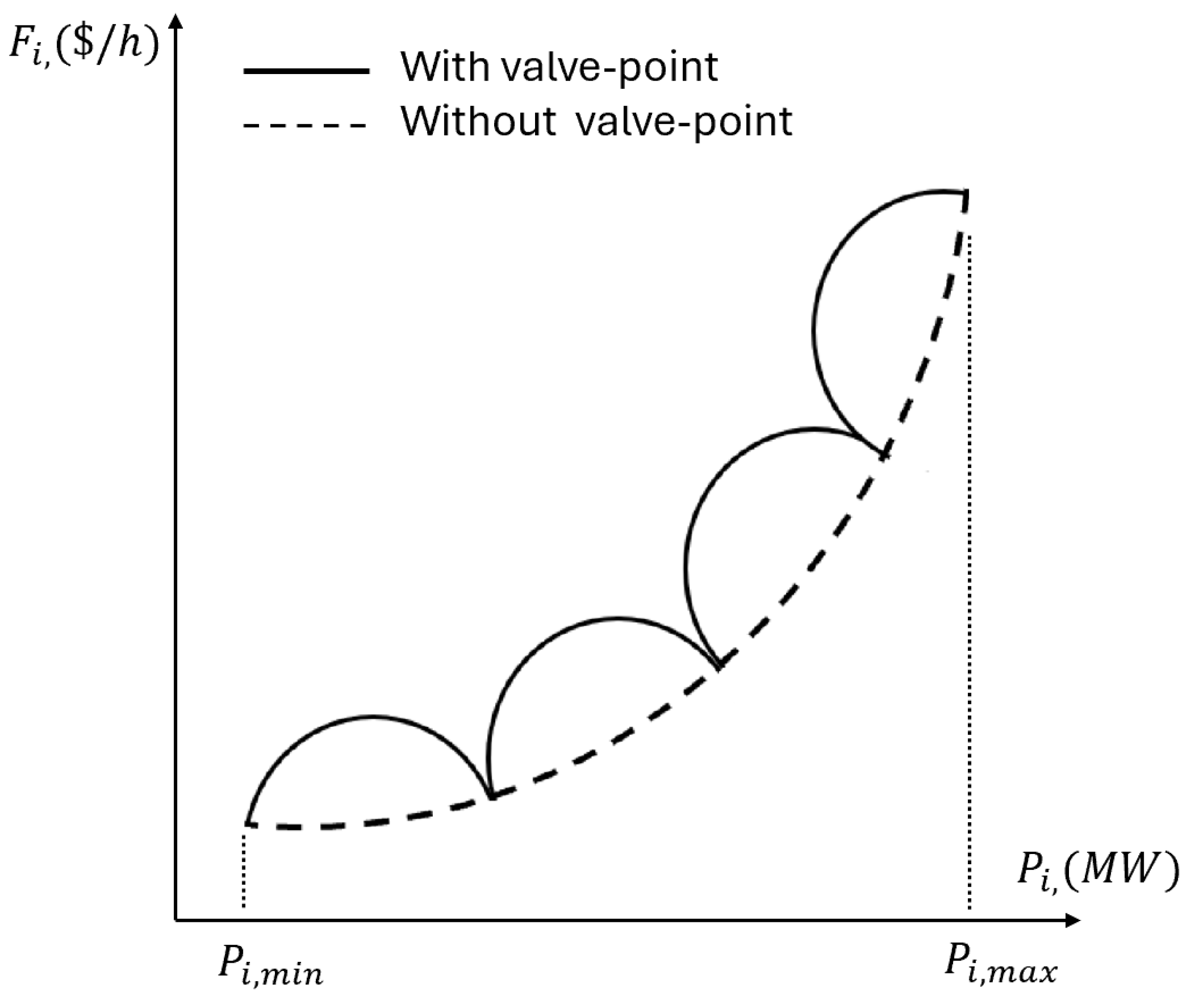
Figure 2.
Convergence characteristics of the proposed GRPO algorithm for the 15-unit test system with prohibited operating zones.
Figure 2.
Convergence characteristics of the proposed GRPO algorithm for the 15-unit test system with prohibited operating zones.
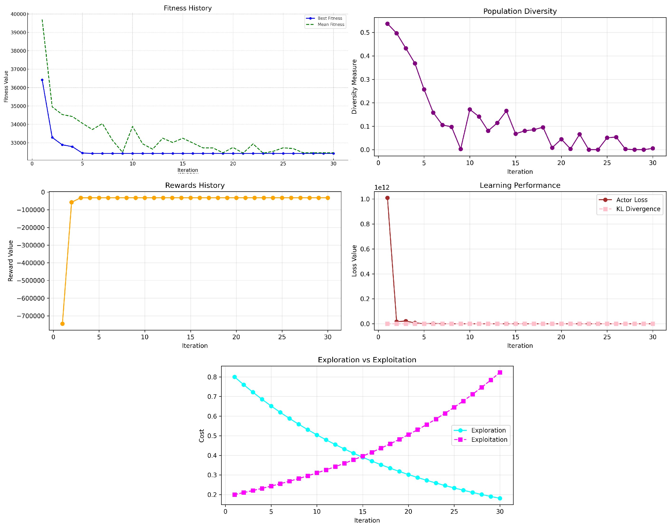
Figure 3.
Optimal power output allocation for each generator in the 15-unit test system using GRPO.
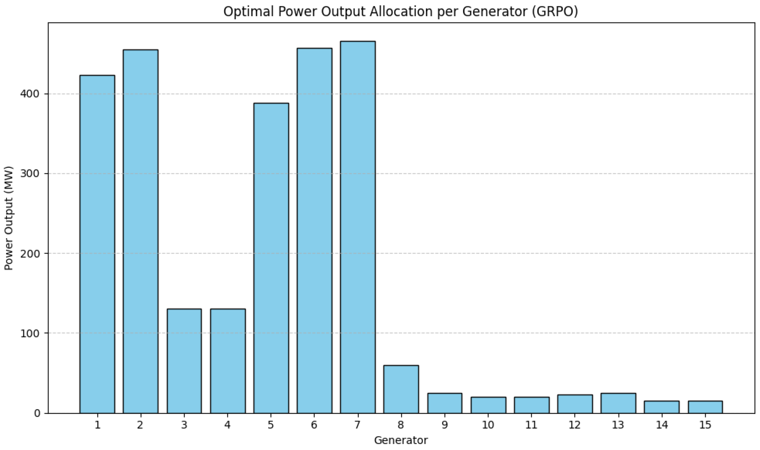
Figure 4.
Performance of the proposed GRPO algorithm for the 30-unit test system with prohibited operating zones.
Figure 4.
Performance of the proposed GRPO algorithm for the 30-unit test system with prohibited operating zones.
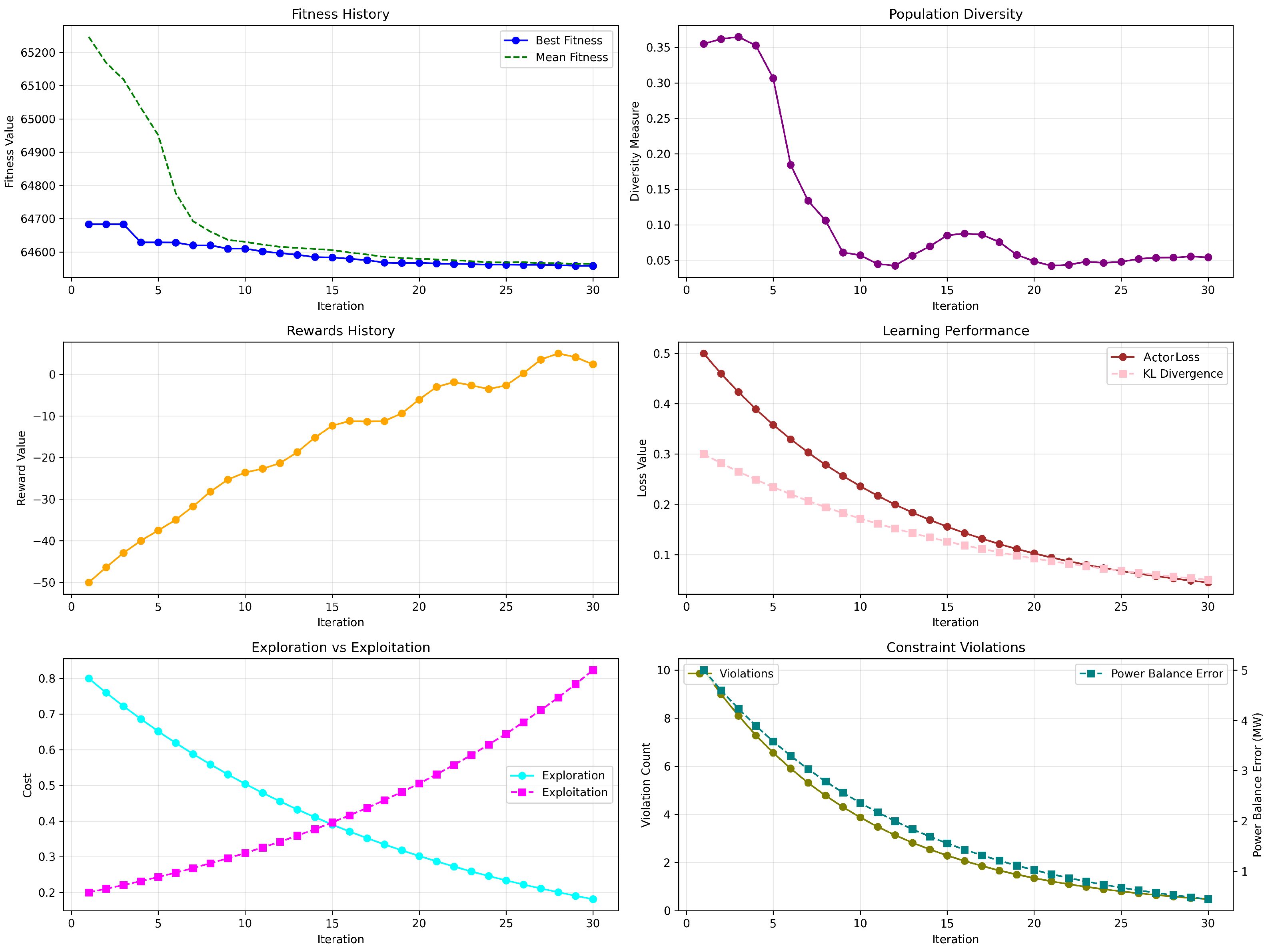
Figure 5.
Performance of the proposed GRPO algorithm for the 60-unit test system with prohibited operating zones.
Figure 5.
Performance of the proposed GRPO algorithm for the 60-unit test system with prohibited operating zones.
Figure 6.
Performance of the proposed GRPO algorithm for the 90-unit test system with prohibited operating zones.
Figure 6.
Performance of the proposed GRPO algorithm for the 90-unit test system with prohibited operating zones.
Table 2.
Optimal power output allocation for the 15-unit test system using GRPO.
| Generator | Power Output (MW) | Generator | Power Output (MW) |
|---|---|---|---|
| 1 | 422.7000 | 9 | 25.0000 |
| 2 | 454.9785 | 10 | 20.0257 |
| 3 | 130.0000 | 11 | 20.0000 |
| 4 | 130.0000 | 12 | 22.5082 |
| 5 | 388.0750 | 13 | 25.0000 |
| 6 | 456.7136 | 14 | 15.0000 |
| 7 | 465.0000 | 15 | 15.0000 |
| 8 | 60.0000 |
Table 3.
Comparison of best cost and computational efficiency for the 15-unit test system with prohibited operating zones.
Table 3.
Comparison of best cost and computational efficiency for the 15-unit test system with prohibited operating zones.
| Method | Best Cost ($/h) | Average Cost ($/h) | CPU Time (s) |
|---|---|---|---|
| GA [18] | 33,113.00 | 33,228.00 | 49.31 |
| PSO [18] | 32,858.00 | 33,039.00 | 26.59 |
| - iterative [25] | 32704.45 | - | - |
| IHNN [26] | 32858.00 | - | - |
| EHNN [27] | 32555.00* | - | - |
| EP [27] | 32715.94 | - | - |
| QEA [28] | 32576.45 | - | - |
| IQEA [28] | 32574.03 | - | - |
| MVMO [29] | 32569.54 | 32572.37 | 9.651 |
| [29] | 32563.58 | 32565.03 | 10.258 |
| GRPO (Proposed) | 32421.67 | 32456.37 | 13.545 |
| *The solution from EHNN is not fully feasible, with 0.8 MW of unallocated power. | |||
Table 4.
Comparisons of average cost and CPU time for different methods and unit sizes
| Method | No. of units | Min cost (best) ($) | Average cost ($) | CPU time (s) |
|---|---|---|---|---|
| MVMO [29] | 30 | 65,086.3370 | 65,090.2023 | 17.051 |
| 60 | 130,170.8046 | 130,175.0956 | 30.030 | |
| 90 | 195,258.6600 | 195,263.5962 | 41.574 | |
| [29] | 30 | 65,086.2051 | 65,089.2153 | 18.096 |
| 60 | 130,170.7797 | 130,175.0130 | 31.325 | |
| 90 | 195,258.4951 | 195,263.5819 | 43.633 | |
| CGA [30] | 30 | - | 65,784.740 | 275.73 |
| 60 | - | 131,992.310 | 563.81 | |
| 90 | - | 198,831.690 | 940.93 | |
| IGAMUM [30] | 30 | - | 65,089.954 | 79.80 |
| 60 | - | 130,180.030 | 162.58 | |
| 90 | - | 195,274.060 | 255.45 | |
| GRPO (Proposed) | 30 | 64558.0856 | 64593.320 | 37.16 |
| 60 | 129217.270 | 129249.667 | 79.98 | |
| 90 | 193936.087 | 194055.320 | 138.14 |
Disclaimer/Publisher’s Note: The statements, opinions and data contained in all publications are solely those of the individual author(s) and contributor(s) and not of MDPI and/or the editor(s). MDPI and/or the editor(s) disclaim responsibility for any injury to people or property resulting from any ideas, methods, instructions or products referred to in the content. |
© 2025 by the authors. Licensee MDPI, Basel, Switzerland. This article is an open access article distributed under the terms and conditions of the Creative Commons Attribution (CC BY) license (http://creativecommons.org/licenses/by/4.0/).
Copyright: This open access article is published under a Creative Commons CC BY 4.0 license, which permit the free download, distribution, and reuse, provided that the author and preprint are cited in any reuse.


