
Submitted:
11 July 2025
Posted:
15 July 2025
You are already at the latest version
Abstract
The rapid growth of the automobile industry has intensified the demand for accurate price prediction models in the used car market. Buyers often struggle to determine fair market value due to the complexity of factors such as mileage, brand, model, transmission type, accident history, and overall condition. This study presents a comparative analysis of machine learning models for used car price prediction, with a strong emphasis on the impact of feature engineering. We begin by evaluating multiple models—including Linear Regression, Decision Trees, Random Forest, Support Vector Regression (SVR), XGBoost, Stacking Regressor, and Keras-based neural networks—on raw, unprocessed data. We then apply a comprehensive feature engineering pipeline that includes categorical encoding, outlier removal, data standardization, and extraction of hidden features (e.g., vehicle age, horsepower). Results demonstrate that advanced preprocessing significantly improves predictive performance across all models. For instance, the Stacking Regressor’s R² score increased from 0.14 to 0.8899 after feature engineering. Ensemble methods such as CatBoost and XGBoost also showed strong gains. This research not only benchmarks models for this task but also serves as a practical tutorial illustrating how engineered features enhance performance in structured ML pipelines for the fellow researchers. The proposed workflow offers a reproducible template for building high-accuracy pricing tools in the automotive domain, fostering transparency and informed decision-making.
Keywords:
feature engineering
; machine learning
; regressor
; price prediction
; car price prediction
; regression
; continuous value prediction
1. Introduction
The used car market has experienced significant growth in recent years, driven by rising consumer demand for affordable transportation and the rise of online car marketplaces. Accurately predicting the price of a pre-owned vehicle is a challenging task due to the numerous factors influencing its value, including mileage, brand, model, transmission type, accident history, and overall condition. Traditional car valuation methods rely on expert assessments or basic statistical models, which often fail to capture the complex, nonlinear relationships among vehicle attributes.
With advancements in machine learning (ML), predictive models have become increasingly effective in estimating used car prices based on historical sales data. This study explores the application of various ML algorithms, including XGBRegressor [1], Stacking Regressor [2], Linear Regression [3,4], Random Forest [5], Support Vector Regression (SVR) [6], and Keras-based neural networks [7], to develop an accurate and scalable price prediction model.
A crucial component of this research is feature engineering [8], which plays a vital role in enhancing model performance. Key transformations applied in our pipeline include:
- Extracting horsepower and engine displacement from engine specification strings.
- Converting categorical features into numerical representations using appropriate encoding techniques.
- Standardizing transmission types via regular expression-based mapping.
- Applying target encoding to brand data based on average vehicle price [9].
- Encoding binary and nominal features using label and binary encoding.
- Identifying and removing statistical outliers [10].
The dataset used in this study [11] contains 4,009 entries and includes attributes such as transmission type, mileage, brand, exterior and interior color, manufacturing year, clean title status, fuel type, accident history, engine details, and selling price. By applying advanced ML techniques to both raw and feature-engineered versions of the data, we aim to build robust models that provide reliable, data-driven price estimations.
By comparing model performance before and after feature engineering, this study offers practical insights into how structured data transformations significantly enhance predictive accuracy. Our findings contribute a reproducible, tutorial-style pipeline applicable to real-world regression tasks in automotive and related domains.
2. Related Work
Several studies have explored machine learning techniques to predict used car prices. However, most focus primarily on model selection, with limited emphasis on the effects of feature engineering. This section reviews representative contributions and highlights how our work advances the state of the art through methodical data transformation and comparative analysis.
Venkatasubbu and Ganesh (2019) applied Lasso, Multiple Regression, and Regression Tree models to a small dataset of 804 records from the Kelley Blue Book. While they reported a high value (0.9927), their dataset lacked diversity and advanced feature processing, limiting generalizability [12].
Zhu (2023) utilized linear regression, decision trees, random forest, and neural networks on U.S. car sales data, employing one-hot encoding for categorical variables. The study achieved reasonable accuracy ( = 0.789 using XGBoost), but did not explore preprocessing techniques beyond basic encoding, nor did it evaluate ensemble strategies [13].
Huang et al. (2023) implemented a model fusion framework incorporating XGBoost, CatBoost, LightGBM, and artificial neural networks, achieving an impressive of 0.9845. However, the feature engineering was limited to forward selection, and no comparison was made between raw and transformed data [14].
Collard (2022) focused on vehicle depreciation modeling using Ridge, Lasso, and Random Forest regressors, along with basic cleaning and normalization. The study did not explore the impact of feature engineering or ensemble modeling [15].
Gupta et al. (2024) and Samruddhi & Kumar (2020) implemented simple pipelines using basic encoding and standard regression or classification models (e.g., KNN). While valuable for introductory applications, these approaches lacked methodological depth and comprehensive comparisons [16].
Bukvić et al. (2022) applied correlation analysis and classification models, reporting strong results (R² = 0.95). However, their modeling pipeline lacked advanced encoding, model stacking, or comparison across preprocessing strategies [17].
In contrast to these studies, our work focuses on quantifying the impact of advanced feature engineering on model performance. We introduce domain-informed transformations such as mileage normalization, car age derivation, transmission standardization using regular expressions, and multiple encoding strategies (label, binary, target). We benchmark over ten models, including tuned versions of XGBoost, CatBoost, LightGBM, SVR, and Stacking Regressor, along with deep neural networks. Our experiments also include execution time comparisons and performance benchmarking both before and after step-by-step comprehensive feature engineering, revealing a substantial improvement in the best-performing model’s score from 0.14 (raw features) to 0.8899 (engineered features).

Table 1.
Comparison of existing studies with the proposed work.
| Study | Feature Engineering | Models Used | R² Score | Remarks |
|---|---|---|---|---|
| Venkatasubbu & Ganesh (2019) | None | Lasso, Regression Tree | 0.9927 | Very small dataset (804 rows) |
| Zhu (2023) | One-hot encoding | Linear, RF, ANN | 0.789 (XGBoost) | No advanced processing |
| Huang et al. (2023) | Forward selection | XGB, CatBoost, ANN | 0.9845 | No raw vs engineered comparison |
| Collard (2022) | Basic cleaning | Ridge, RF | Not stated | Depreciation model focused |
| Gupta et al. (2024) | Basic encoding | Linear, Classifiers | Not stated | Focus on transparency |
| Samruddhi & Kumar (2020) | Simple preprocessing | KNN | ∼0.85 | Small-scale demonstration |
| Bukvić et al. (2022) | Correlation only | Linear Regression | 0.95 | Limited modeling diversity |
| Our Work | Advanced (regex, encodings, scaling) | 10+ models incl. Stacking | 0.8899 | Comprehensive comparison, before/after feature engineering |
This review highlights a consistent gap in prior research—limited feature engineering and an absence of pipeline-level comparisons. Our contribution addresses this gap through a complete modeling framework that incorporates feature transformation, model optimization, and evaluation of deep learning and ensemble techniques under varying preprocessing conditions.
To further illustrate the performance improvements enabled by feature engineering, Figure 1 presents a visual comparison of scores across the relevant evaluated models, both before and after applying transformation techniques. The plot clearly demonstrates that ensemble-based models—particularly Stacking Regressor, CatBoost, and XGBoost—benefited significantly from structured preprocessing, achieving the highest performance gains. Even simpler models, such as Linear Regression , showed measurable improvement following feature enhancement. The later part of the paper demonstrates how the feature engineering is done on the messy publicly available data set and improve the prediction performance dramatically.
3. Materials and Methods
The pre-owned cars dataset was taken from Kaggle [11]. To get the accurate car price prediction, we have performed an extensive feature engineering including filtering and removing unnecessary data, converting textual data to numerical form, removing outliers and finding important features through correlations [18]. The summary of the work done is shown in a data flow diagram in Figure 2.
4. Exploratory Analysis
4.1. Dataset
We have collected the freely available pre-own car dataset from Kaggle [11]. The dataset consists of 4,009 records with 12 features, representing key attributes influencing the price of used cars.
The dataset includes the following attributes:
- Brand: Categorical representation of car brands.
- Mileage: The total distance the car has traveled.
- Fuel Type: Encoded as integers, representing fuel categories (e.g., Petrol, Diesel, other, etc.).
- Transmission: Encoded as integers, indicating Manual or Automatic transmission.
- Exterior Color & Interior Color: Coded numerical representations of car colors.
- Accident History: Indicates whether the car has been involved in an accident (binary feature).
- Clean Title: A binary feature indicating whether the car has a clean ownership record.
- Price: The target variable representing the selling price of the vehicle.
- Age: The number of years since the car’s manufacture.
- Horsepower: The power output of the car’s engine.
- Engine Displacement: The engine size, measured in liters.
4.2. Graphical Analysis
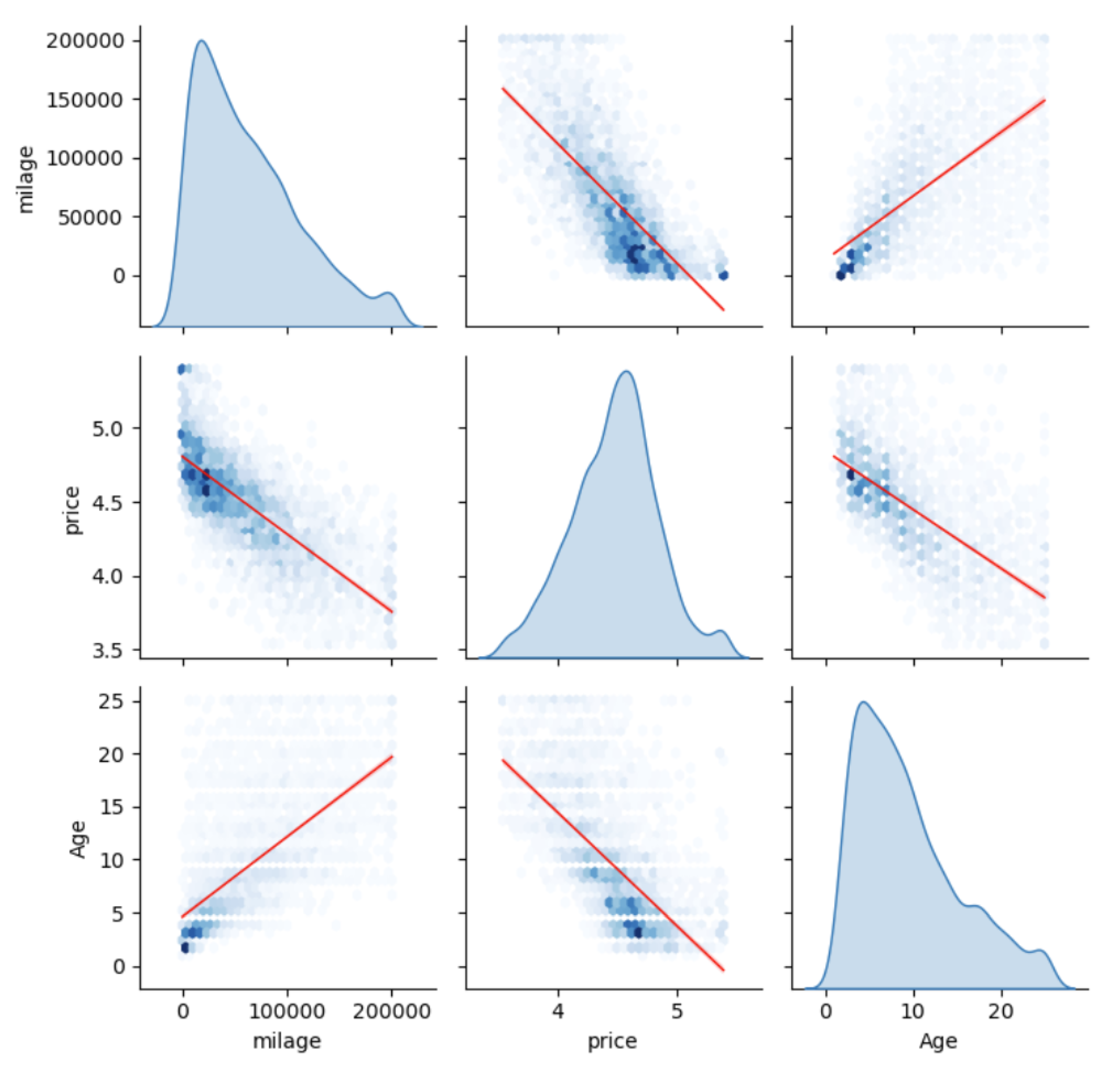
To visually explore relationships between features, we generated a pair plot (Figure 3) and a correlation heatmap (Figure 5). These visualizations highlight the most influential variables affecting vehicle price, including age and mileage, which show strong negative correlations.
4.2.1. Pairplot
To gain a better understanding of the dataset, visualizations were produced for the significant features [19]. A pair plot was generated for price, age, and mileage to observe the relationships between these numerical features. The plot demonstrates expected trends, such as some cars having higher mileage and prices and vice versa.
Figure 3.
Pair plot showing relationships between price, age, and mileage.
4.2.2. Correlation Analysis: Before and After Feature Engineering
To understand the impact of feature engineering, we analyzed Pearson correlations between features and price before and after transformation.
Figure 4 shows the correlation matrix using minimally processed data. As shown, the relationships with price are weak or misleading due to unstandardized formats, missing values, and unencoded categorical variables. For example:
- Mileage has a weak negative correlation with price ().
- Model year shows only a weak positive correlation ().
- Brand, fuel type, color, and transmission exhibit near-zero correlation due to inconsistent encoding and categorical noise.
- Horsepower and engine data were not yet extracted, so they don’t contribute meaningfully.
Figure 4.
Correlation heatmap before feature engineering. Most relationships with price are weak or noisy due to unprocessed categorical and textual features.
Figure 4.
Correlation heatmap before feature engineering. Most relationships with price are weak or noisy due to unprocessed categorical and textual features.
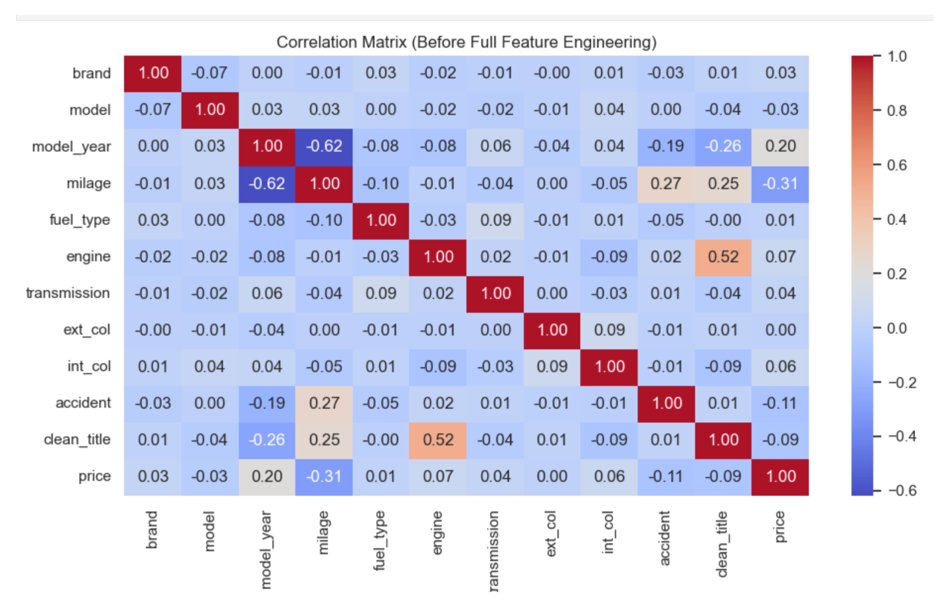
Figure 5 shows the correlation matrix after full preprocessing and feature engineering. Key improvements include:
- Mileage now shows a strong negative correlation with price (), confirming that higher mileage reduces car value.
- Age exhibits a strong negative correlation (), as expected.
- Horsepower has a strong positive correlation (), now accurately extracted from engine specifications.
- Brand also correlates well (), reflecting the effect of target encoding.
- Engine displacement also correlates moderately with price ().
- Accident history and manual transmission now show clearer negative correlations ( to ).
Figure 5.
Correlation heatmap after full feature engineering. Stronger, more interpretable relationships emerge between features and price.
Figure 5.
Correlation heatmap after full feature engineering. Stronger, more interpretable relationships emerge between features and price.
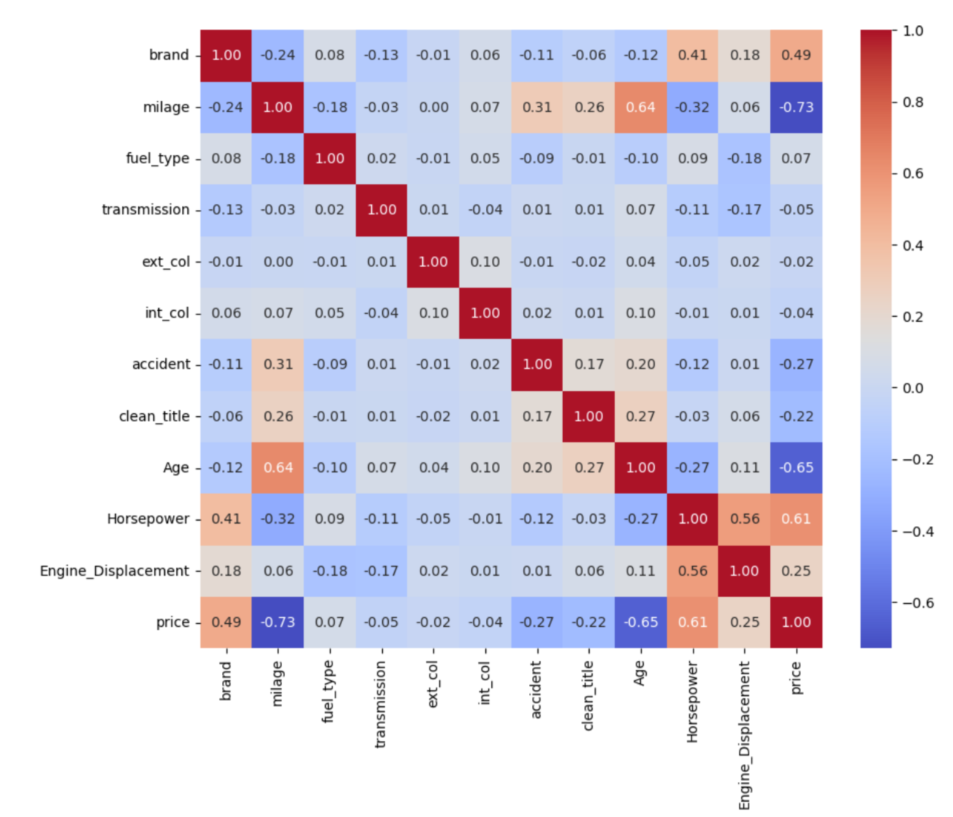
These improvements validate the importance of structured feature engineering for meaningful pattern extraction in tabular ML tasks.
4.2.3. Brand Variance
Figure 6 shows the distribution of car manufacturers in the dataset. The brand feature was target-encoded, meaning each brand was assigned a numeric value based on its average vehicle price. This transformation helps the model capture brand-specific pricing trends more effectively.
The most frequently represented brands are Ford, BMW, and Mercedes-Benz, indicating strong market presence and demand. Other well-represented brands include Chevrolet, Porsche, and Toyota. In contrast, premium manufacturers such as Bugatti, Rolls-Royce, and Maybach appear infrequently, likely due to their high price and limited availability.
This results in a long-tail distribution — a small number of brands dominate the dataset, while many others have minimal representation. Such imbalance can potentially affect the model’s ability to generalize pricing patterns across less common manufacturers.
Figure 7 displays the feature importance derived from correlation coefficients with the target variable, vehicle price. Positive correlations indicate features that increase with price, such as horsepower and brand, while negative correlations reflect inverse relationships. Notably, mileage and age exhibit strong negative correlations (-0.70 and -0.60, respectively), confirming that older, high-mileage vehicles tend to be priced lower. In contrast, horsepower shows a strong positive correlation, aligning with market expectations that more powerful vehicles command higher prices. Categorical features like fuel type, transmission, and interior/exterior color show relatively weaker correlations, suggesting that their influence is either more nuanced or captured through interaction with other variables. This correlation-based ranking guided our selection and transformation of features during the engineering phase.
4.3. Impact of Feature Engineering on Model Performance
To further quantify the effectiveness of feature engineering, we evaluated five regression models on both raw and fully processed datasets. Figure 8 presents a side-by-side comparison of scores before and after feature transformation.
The results highlight a substantial improvement in predictive performance across all models. Linear Regression improved from an of just 0.03 to 0.79, while Stacking Regressor achieved a leap from 0.15 to 0.88. Ensemble models such as CatBoost and XGBoost also showed significant gains, reinforcing the value of structured preprocessing.
5. Feature Engineering
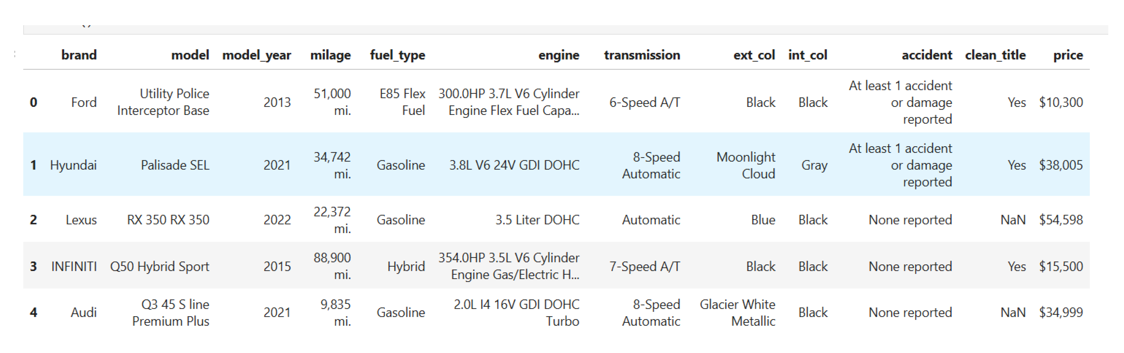
This figure shows a sample of the original dataset, including key features such as brand, model, mileage, fuel type, engine specification, transmission, color, accident history, and price. As evident, the raw data contains inconsistent formats, categorical text, and missing values, which makes it unsuitable for direct application of machine learning algorithms.
Figure 9.
Raw data from the dataset [11] which is not readily available for applying machine learning algorithms.
Figure 9.
Raw data from the dataset [11] which is not readily available for applying machine learning algorithms.
To address this, comprehensive preprocessing and feature engineering are required. In the following steps, we detail how the dataset was transformed into a structured, model-ready format.
Predicting the price of a pre-owned vehicle is a complex task influenced by multiple factors such as brand, mileage, accident history, transmission type, and engine specifications. Feature engineering plays a crucial role in transforming raw data into meaningful features. These transformations improve the model’s ability to make accurate predictions.
This process involves multiple steps:
- Data Cleaning – Handling missing values, correcting inconsistencies, and ensuring data quality [20].
- Feature Transformation – Converting categorical variables into numerical values and normalizing numerical features.
- Feature Selection – Identifying the most relevant variables that contribute to price prediction.
- Outlier Detection & Handling – Removing or adjusting anomalies that may skew predictions.
- Feature Scaling – Standardizing or normalizing features for better model performance [21].
5.1. Importance of Feature Engineering in Car Price Prediction
- Well-engineered features help machine learning models detect patterns more effectively.
- Cleaning and transforming data removes irrelevant details that could mislead the model.
- Domain-specific feature engineering (e.g., converting color names into standard categories) makes the model insights more understandable.
- Used car data often contains missing values, inconsistent entries, and outliers, requiring proper preprocessing.
In our car dataset features fall into the following two categories:
5.1.1. Numerical Features
- Mileage (higher mileage often reduces value)
- Age of the Car (older cars generally have lower prices)
- Horsepower (higher power may indicate a more expensive car)
- Engine Displacement (larger engines often correlate with higher prices)
5.1.2. Categorical Features
- Brand & Model (premium brands tend to hold value better)
- Transmission Type (automatic cars are often priced differently from manual ones)
- Fuel Type (diesel, petrol, electric—each has different market demand)
- Exterior & Interior Color (some colors retain value better)
- Accident History (cars with reported accidents tend to be cheaper)
- Clean Title (a clean title means no major past issues, which impacts pricing)
5.2. Handling Missing Values
Certain features contained missing values, which were handled as follows:
- Fuel Type: Missing values in the fuel type column were replaced with “not supported.” Additionally, any invalid characters, such as “–,” were standardized to “not supported” for consistency.
- Clean Title: If the clean title information was missing, it was assumed that the vehicle does not have a clean title, so the missing values were replaced with “no.”
- Accident Reports: When accident history data was unavailable, the missing values were replaced with “None reported,” assuming no reported incidents.
5.3. Data Standardization
To maintain uniformity and facilitate analysis, certain numerical fields were converted into a consistent format:
- Mileage: Originally stored as a string with units such as “mi.” and commas, mileage values were stripped of these characters and converted into a numerical format.
- Price: The price field, initially stored as a string containing dollar signs and commas, was cleaned by removing these symbols and converted into a numerical format.
5.4. Calculating Vehicle Age
Since the model year provides insight into the vehicle’s age, this value was transformed by subtracting it from the current year. After deriving the age, the model year column was removed, as it was no longer necessary.
5.5. Price Transformation
To normalize price distribution and minimize skewness, a logarithmic transformation was applied. This adjustment ensures that price data is more normally distributed, improving the performance of machine learning models that assume normality in input features.
5.6. Feature Engineering: Transmission
5.6.1. Primary Standardization
Raw transmission data presented numerous variations (e.g., “6-Speed A/T”, “8-Speed PDK”, “CVT-F”) requiring standardization. A detailed mapping dictionary consolidated these variations into three main categories:
- Automatic: Including standard automatics, dual-clutch systems, and CVTs
- Manual: Encompassing all manual transmissions regardless of speed configuration
- Other: Capturing variable transmissions and non-standard configurations
5.6.2. Consistency Enhancement
A secondary function was created for classification:
- Identifying “Automatic” keywords for automatic transmissions
- Detecting “Manual” indicators for manual transmissions
- Defaulting unmatched cases to “Other”
5.6.3. Numerical Encoding
Final transformation converted categories to numerical values:
5.6.4. Benefits
The implemented approach provided multiple advantages:
- Reduced dimensionality while preserving transmission type distinctions
- improved data quality through standardization
- Improved model interpret-ability
- Improved the correlation with price
This approach successfully transformed complex transmission descriptions into a simplified, model-ready feature while preserving essential information for price prediction.
5.7. Feature Engineering: Engine
5.7.1. Data Extraction
Raw engine data contained multiple specifications within a single string (e.g., "2.0L 255HP", "1.8 Liter Turbo"), requiring structured parsing to extract key numerical attributes:
- Horsepower: Extracted from descriptions containing HP indicators, representing the vehicle’s power output.
- Engine Displacement: Measured in liters, representing the total volume of the engine’s cylinders.
To systematically extract these values, Regular Expressions (Regex) were employed due to their efficiency in pattern recognition within text-based datasets.
5.7.2. Regex-Based Parsing and Standardization
Regex [22] patterns were designed to extract the numerical values corresponding to horsepower and displacement:
Horsepower Extraction:
- Regex Pattern:(\d+d+)HP|\d+d+
- This pattern captures numeric values preceding an “HP” indicator or standalone decimal values signifying horsepower.
- Example: From "2.0L 255HP", the pattern extracts 255 as horsepower.
Engine Displacement Extraction:
- Regex Pattern:(\d+d+L|\d+d+ Liter)
- This pattern identifies values followed by “L” or “Liter,” ensuring proper detection of engine displacement.
- Example: From "1.8 Liter Turbo", the pattern extracts 1.8 as engine displacement.
These extracted values were then subjected to data preprocessing:
- Removal of unit indicators (e.g., "L", "Liter") for displacement.
- Conversion to numerical format for both attributes.
- Imputation of missing values using mean-based techniques.
5.7.3. Numerical Encoding
Final transformation ensured compatibility with numerical models:
Where:
- Horsepower: Extracted and imputed as needed.
- Engine Displacement: Converted to numerical format.
5.7.4. Benefits
The use of regex-based feature extraction provided multiple advantages:
- Automated parsing of complex engine descriptions, eliminating manual intervention.
- Standardization of measurement units for consistent data representation.
Raw textual engine specifications were efficiently transformed into structured numerical features, ensuring they are utilized fully in making prediction.
5.8. Feature Engineering: Interior and Exterior Color
5.8.1. Color Consistency
Color normalization is essential in data processing to standardize categorical attributes and improve dataset consistency. In automotive datasets, color descriptions often vary due to manufacturer naming conventions and subjective marketing terms. Standardization ensures that similar colors are grouped under common labels, reducing variability and enhancing data quality.
5.8.2. Categorization
A predefined set of base colors provides a structured framework for classification. This approach simplifies analysis and ensures uniform representation across different sources. Any descriptions that do not match predefined categories are assigned to an "other" category to maintain data integrity.
5.8.3. Benefits
- Eliminates inconsistencies in color descriptions.
- Facilitates accurate comparisons and analyses.
- Enhances compatibility with machine learning models by reducing feature sparsity.
By applying systematic categorization techniques, color normalization transforms unstructured textual attributes into meaningful and standardized data, improving the overall reliability of analytical models.
5.9. Outlier Detection and Treatment
Outlier detection is a crucial preprocessing step in data analysis that ensures data consistency and prevents extreme values from distorting statistical analyses and machine learning models. The Interquartile Range (IQR) method is a widely used technique to identify and handle outliers effectively.
5.9.1. Interquartile Range (IQR) Method
The IQR method identifies outliers based on the spread of the middle 50% of the data. The first quartile (Q1) and third quartile (Q3) define the interquartile range, calculated as:
Values falling below or above are considered outliers and are adjusted accordingly.
5.9.2. Normalization
The IQR method is applied to multiple numerical attributes in automotive datasets, such as:
- Age: Standardizing vehicle age to remove extreme values.
- Price: Ensuring consistency in vehicle pricing distribution.
- Mileage: Preventing extreme mileage values from skewing predictions.
- Horsepower: Normalizing horsepower values to maintain reliable model inputs.
- Engine Displacement: Eliminating anomalies in engine specifications.
5.9.3. Benefits
Applying the IQR-based approach offers multiple advantages:
- Improves the robustness of statistical analysis.
- Enhances the performance of machine learning models by reducing noise.
- Ensures a more accurate representation of data trends.
- Prevents extreme values from distorting prediction outcomes.
By systematically detecting and adjusting outliers, datasets achieve better consistency, reliability, and usability in predictive modeling and statistical evaluations.
5.10. Categorical Data Encoding
5.10.1. Theoretical Background
Categorical data encoding is essential in transforming non- numeric features into a numerical format suitable for machine learning models. Encoding techniques ensure that categorical variables contribute effectively to model performance while preserving interpretability.
5.10.2. Feature Encoding Methods
Various encoding techniques were applied to different categorical attributes in the dataset:
-
Binary Encoding: Used for boolean variables such as accident history and clean title, where values were mapped as follows [23]:
- -
- Accident History: "At least 1 accident or damage reported" → 1, "None reported" → 0.
- -
- Clean Title: "Yes" → 1, "No" → 0.
- Label Encoding: Applied to categorical attributes with a clear ordinal structure, such as fuel type, exterior color, and interior color, to convert them into numerical representations [24].
- Target Encoding: Initially, one-hot encoding was used for the brand attribute. However, due to a lack of correlation with price, target encoding was implemented instead. This technique captures the relationship between categorical variables and a target variable (price), enhancing model performance [25].
5.10.3. Benefits
By applying appropriate encoding methods, the following advantages were achieved:
- Improved compatibility with machine learning models.
- Reduction in feature dimensionality by avoiding unnecessary expansion.
- Better representation of categorical variables in relation to predictive outcomes.
By systematically encoding categorical features, the dataset was transformed into a structured numerical format, ensuring optimal performance in predictive modeling.
6. Train Test Split
The train-test split is a fundamental step in machine learning that ensures unbiased model evaluation. By dividing the dataset into distinct training and testing subsets, the model’s ability to generalize to unseen data can be effectively assessed. This prevents overfitting and provides a reliable estimate of model performance [26].
Dataset Partitioning
The dataset was divided into two subsets:
- Training Set: Comprising 80% of the data, used for model training and learning patterns.
- Testing Set: The remaining 20%, used to evaluate model performance on unseen data.
This balanced split ensures the model learns meaningful patterns without overfitting and maintains strong performance on previously unseen data.
7. Machine Learning Algorithms
This section discusses the various machine learning algorithms utilized in the prediction model for vehicle pricing.
7.1. Linear Regression Performance Analysis
Linear regression is a fundamental algorithm used to establish a linear relationship between dependent and independent variables. It assumes a straight-line relationship and is useful for interpreting feature importance through coefficient values. It was used as a baseline predictor for vehicle price, trained on a scaled feature set and evaluated using normal regression metrics. The model achieved a Root Mean Squared Error (RMSE) of 0.1634, reflecting a very small difference between predicted and actual prices [27]. Most importantly, the R2 Score [28] was 0.7983, indicating that approximately 79.8% of the variation in car prices is accounted for by the features used in the model. This suggests that Linear Regression provides a solid baseline, although ensemble models might yield better results.
Support Vector Regression (SVR) Performance Analysis
Support Vector Regression (SVR) is an extension of Support Vector Machines (SVM) for regression tasks. It employs a kernel trick to capture non-linearity in data, making it effective for complex relationships between vehicle attributes and price.
SVR was employed as part of the predictive modeling process for car price prediction, trained on the scaled dataset and evaluated using standard regression metrics. The Root Mean Squared Error (RMSE) was 0.1447, indicating minimal deviation between predicted and actual prices. Most importantly, the R2 Score was 0.8419, meaning that approximately 84.19% of the variance in car prices is explained by the model. This highlights SVR’s effectiveness in modeling non-linear relationships, showing a notable improvement over linear regression models.
7.2. Random Forest Regression and Performance Analysis
Random Forest is an ensemble learning method that constructs multiple decision trees and aggregates their predictions to enhance accuracy. It mitigates overfitting and effectively captures non-linear dependencies in datasets, making it well-suited for prediction tasks.
In this study, Random Forest Regression was employed for vehicle price prediction, using 150 estimators (n_estimators) to achieve robust performance through the averaging of predictions. The model achieved a Root Mean Squared Error (RMSE) of 0.1313, indicating minimal variation between predicted and actual prices. Furthermore, the R2 score of 0.8697 demonstrates that approximately 86.97% of the variance in car prices is explained by the model, underscoring the effectiveness of ensemble methods in tackling complex regression problems.
7.3. XGBoost Regression and Performance Analysis
XGBoost is an optimized version of gradient boosting, renowned for its speed, performance, and ability to handle missing values, feature interactions, and non-linearity. These attributes make it a robust choice for price prediction tasks.
In this study, XGBoost Regression achieved a Root Mean Squared Error (RMSE) of 0.1262, reflecting minimal deviation between predicted and actual prices. Additionally, the score of 0.8798 indicates that 87.98% of the variance in vehicle prices is explained by the model’s input features, highlighting its effectiveness in capturing complex patterns and delivering highly accurate predictions.
7.4. Stacking Regressor and Performance Analysis
Stacking Regressor is an ensemble learning technique that combines multiple base models to enhance predictive accuracy. It utilizes a meta-model trained on the predictions of individual estimators to leverage their combined strengths. The stacked model in this study included the following estimators: SVR (C=10, gamma=0.1, epsilon=0.1), Random Forest (n_estimators=500, max_depth=10), and XGBoost (n_estimators=500, learning_rate=0.05).
The model achieved a Root Mean Squared Error (RMSE) of 0.1208, demonstrating minimal deviation between predicted and actual prices. Furthermore, the score of 0.8899 indicates that 88.99% of the variance in vehicle prices is explained by the input features, showcasing the superior performance of the Stacking Regressor in capturing complex patterns and delivering accurate predictions.
7.5. XGBRegressor with Grid Search and Performance Analysis
XGBRegressor, a core implementation of XGBoost, was employed in both base form and with hyperparameter tuning via GridSearch to enhance model performance [29]. Grid Search Cross Validation was used to optimize key parameters, evaluating 729 parameter combinations across 3 cross-validation folds. The best parameters were identified as follows: colsample_bytree = 0.8, learning_rate = 0.1, max_depth = 5, min_child_weight = 1, n_estimators = 300, and subsample = 1.0.
Using these optimized parameters, the retrained model was evaluated and achieved a Root Mean Squared Error (RMSE) of 0.1213, indicating minimal deviation from actual car prices. The score of 0.8888 illustrates that 88.88% of the variance in vehicle prices is explained by the model’s input features, confirming the effectiveness of the optimized XGBRegressor in capturing complex patterns and providing accurate predictions.
7.6. Keras Regression and Performance Analysis
Keras Regression leverages deep learning to capture complex patterns for price prediction. The model architecture comprised a sequential neural network with the following configuration: Input layer (12 neurons, ReLU activation), Hidden layer (8 neurons, ReLU activation), Hidden layer (4 neurons, ReLU activation), and Output layer (1 neuron for regression). The network was trained using the Adam optimizer with a loss function of Mean Squared Error (MSE), over 100 epochs with a batch size of 64, and validated on the test set.
The model achieved a Root Mean Squared Error (RMSE) of 0.1602, indicating a small deviation between predicted and actual prices. The score of 0.8061 indicates that 80.61% of the variance in car prices is explained by the input features. While the results are reasonable, optimizing hyperparameters, refining the network architecture, or improving training strategies could further enhance the model’s performance.
7.6.1. Early Stopping and Dropout Techniques
Early stopping prevents overfitting by halting training once validation performance stops improving, while dropout randomly deactivates neurons during training, enhancing model generalization by reducing reliance on specific features.
Neural Network Architecture with Early Stopping and Dropout: The model followed the previous Keras architecture, but dropout layers with a rate of 30% were added after each dense layer. Early stopping was configured to monitor validation loss, stopping training after 10 epochs of no improvement. The model was compiled using the Adam optimizer with a Mean Squared Error (MSE) loss function. Training was conducted for a maximum of 100 epochs with a batch size of 64, but early stopping ensured efficiency.
The architecture was as follows: Input layer (12 neurons, ReLU activation + 30% dropout), Hidden layer (8 neurons, ReLU activation + 30% dropout), Hidden layer (4 neurons, ReLU activation + 30% dropout), and Output layer (1 neuron for regression).
Performance Metrics: The model achieved a Root Mean Squared Error (RMSE) of 0.2950, showing a significant deviation between predictions and actual values, and an score of 0.3429, indicating that only 34.29% of the variance in car prices was explained by the input features. While dropout and early stopping effectively reduced overfitting, the overall predictive performance was significantly weaker compared to other approaches.
7.6.2. Analysis of Deep Learning Underperformance
Despite its success in vision and language tasks, deep learning models often underperform on small, structured tabular datasets. In our study, a Keras-based neural network was compared against tree-based regressors for used car price prediction. The deep model consistently lagged behind, and the reasons are outlined below.
Data Size and Complexity: Neural networks require large datasets to generalize effectively. With approximately 4,000 samples, the dataset was insufficient for the network to learn robust patterns, whereas tree-based models such as XGBoost and stacking regressors handled this scale well.
Categorical Feature Handling: Although encoding techniques (e.g., target encoding) were applied, the deep model struggled to extract meaningful relationships from categorical inputs. In contrast, tree-based models natively process such features more effectively.
Overfitting: Regularization methods (dropout, early stopping) were used, yet the model showed signs of overfitting and poor generalization. Due to the data being low, the dropout was a bad implementation.
Performance Comparison: Deep learning performance was inconsistent, with R² scores ranging from 0.34 to 0.79 and RMSE up to 3.79, far behind the ensemble-based approaches.
Conclusion: Tree-based models remain better suited for small, structured datasets. Future work may investigate hybrid architectures combining deep learning for feature extraction with tree-based regressors for prediction.
7.7. LightGBM Performance Analysis
LightGBM (Light Gradient Boosting Machine) is an efficient and fast boosting algorithm designed for large datasets. It achieves high accuracy while maintaining computational efficiency [30].
Model Training and Performance Analysis: LightGBM was trained on the scaled dataset using default hyperparameters. Upon evaluation, the model demonstrated a Root Mean Squared Error (RMSE) of 0.1257, reflecting minimal deviation from true price values. The Score of 0.8806 shows that 88.06% of the variance in vehicle prices was explained by the input features. These results highlight LightGBM as an efficient and competitive ensemble-based technique for regression tasks.
7.8. CatBoost
CatBoost is a gradient boosting algorithm specifically optimized for categorical data. It natively handles categorical features without extensive preprocessing, making it particularly effective for structured datasets [31].
Model Training and Performance Analysis: CatBoost Regressor was trained on the scaled dataset with default parameter settings. The model achieved a Root Mean Squared Error (RMSE) of 0.1212, indicating high prediction accuracy with minimal deviation from true values. The Score of 0.8890 highlights that 88.90% of the variance in car prices was explained by the input features. These results establish CatBoost as one of the most effective models in this study, outperforming traditional regression approaches and several ensemble techniques.
7.9. Comparison Table
Table 2 summarizes the final performance of all evaluated regression models after applying the full feature engineering pipeline. The results are reported using two complementary metrics: RMSE (root mean squared error) and R2 score.
Among all models, the Stacking Regressor achieved the best overall performance, with an RMSE of 0.1208 and an R2 score of 0.8899. Tree-based ensemble models like CatBoost and XGBoost (with or without Grid Search) followed closely, demonstrating strong predictive power with RMSE values around 0.12 and R2 scores above 0.88.
LightGBM and Random Forest also performed well, showing slightly higher errors but maintaining strong R2 scores above 0.86. SVR and the Keras-based neural network achieved moderate performance, with RMSE values of 0.1447 and 0.1602, respectively. Although their R2 scores remain above 0.80, they fall short of the ensemble methods.
Linear Regression, while still the simplest model, improved significantly after preprocessing, achieving an R2 of 0.7983. However, deep learning models incorporating dropout and early stopping showed the weakest performance, likely due to underfitting or insufficient optimization, with an RMSE of 0.2950 and an R2 of just 0.3429.
These results highlight the strength of ensemble tree-based methods on structured tabular data and underscore the importance of both preprocessing and model selection in achieving high predictive accuracy.
While all regression models listed in Table 2 were trained and evaluated under the same pipeline, only a subset of five was selected for detailed before-and-after comparison in Table 3. These models—Linear Regression, Random Forest, XGBRegressor (Base), CatBoost, and the Stacking Regressor—were chosen based on three key criteria:
- Architectural diversity: The selected models span a spectrum of complexity, ranging from simple linear models (Linear Regression) to ensemble tree-based methods (Random Forest, XGBoost, CatBoost) and meta-learners (Stacking Regressor). This variety allows for a more generalizable understanding of how feature engineering affects different model classes.
- Interpretability and reliability: These models produced consistently interpretable results with stable performance across runs, making them ideal candidates for a controlled comparison. In contrast, models like SVR and Keras-based neural networks exhibited high sensitivity to hyperparameters, slower training, or inconsistent behavior, which would complicate a fair before-and-after analysis.
- Analytical clarity: Including all models in before-and-after plots would introduce visual clutter and diminish readability without offering additional insights. The selected models sufficiently represent the performance trends observed across the broader set.
This focused comparison enables clearer visualization of the impact of feature engineering while maintaining methodological rigor.
7.10. Model Performance Comparison
To visually compare the performance of different regression models, we plotted their R2 and RMSE scores side by side. Figure 10 illustrates both how well each model explains the variance in vehicle prices (R2) and their average prediction error (RMSE).
From Figure 10, it is evident that ensemble models like Random Forest, XGBoost, and the Stacking Regressor consistently outperform simpler models such as Linear Regression and Support Vector Regression (SVR). These ensemble methods excel at capturing nonlinear feature interactions, managing multicollinearity, and handling feature noise — all of which are crucial in real-world, heterogeneous datasets like used car listings.
In contrast, simpler models such as Linear Regression lack the capacity to model complex relationships unless supported by extensive feature engineering, and SVR, while more flexible, can be sensitive to feature scaling and hyperparameter tuning. Meanwhile, deep learning models, though highly expressive, underperformed due to the relatively small dataset size and the nature of tabular, structured data, which typically favors decision-tree-based methods over neural architectures. These results reaffirm the strength of ensemble regressors as a default choice for tabular regression tasks, especially when combined with thoughtful feature transformations.
7.11. Time Comparison
Figure 11 presents the execution time for each regression model. As expected, simple models like Linear Regression and base XGBRegressor complete training in under a second. Tree-based models such as Random Forest and CatBoost remain relatively efficient, while ensemble methods like the Stacking Regressor and XGBoost with GridSearch exhibit the highest training time—over 30 seconds in some cases.
Deep learning models, including Keras Regression with dropout and early stopping, also show longer execution times due to iterative training and validation monitoring. Interestingly, techniques like early stopping, while reducing overfitting, introduce additional training overhead.
This analysis highlights an important trade-off: while complex models tend to offer better accuracy, they often come at a significantly higher computational cost. For deployment in real-time systems or large-scale platforms, these time differences could affect scalability. Future work may explore more efficient stacking frameworks, model pruning, or distillation to reduce inference time without compromising performance.
8. Comparative Analysis: With vs. Without Feature Engineering
Feature engineering plays a critical role in enhancing the predictive power of machine learning models, particularly when working with structured tabular datasets. To quantify its impact, we conducted a comparative study using two configurations: one using only minimal preprocessing, and the other incorporating a comprehensive feature engineering pipeline.
In the baseline setup, categorical variables were left largely untouched or processed using simple label encoding without accounting for cardinality or relationship to the target. Additionally, no derived features or transformations were introduced. As a result, most models struggled to capture underlying patterns. For instance, Random Forest and XGBoost achieved R² scores between 0.12 and 0.14, and RMSE values exceeding 133,000. Linear Regression performed worst, with an R² of just 0.03—highlighting its inability to model nonlinear relationships in raw tabular data (See Figure 12 and Figure 8).
By contrast, the final version of the dataset underwent extensive feature engineering, which proved transformative. Key techniques included:
- Categorical encoding: High-cardinality fields such as brand and model were encoded using target encoding and frequency-based grouping, improving alignment with the target variable.
- Outlier removal: Abnormal values in price, mileage, and horsepower were filtered using interquartile range (IQR) logic to reduce noise and variance.
- Normalization: Continuous features were scaled to stabilize gradient-based learning and improve model convergence.
- Feature extraction: Additional features such as car age, engine displacement, and power-to-weight ratios were derived from raw attributes, enhancing feature richness.
These transformations resulted in substantial performance gains. For example, the Stacking Regressor improved from an R² of 0.1486 to 0.8899 and achieved an RMSE of just 0.1208. XGBoost and Random Forest also exhibited significant improvements, outperforming their baseline results by a large margin.
Linear models showed the greatest relative improvement due to their reliance on properly scaled, transformed inputs. Ensemble tree-based models, though more robust, still benefited greatly from the clearer signal provided by the engineered features.
The findings underscore that feature engineering is not merely a supporting step, but a critical component of predictive modeling in structured domains. In many real-world scenarios, enhancing data representation may yield greater improvements than algorithm selection or hyperparameter tuning. Future work should continue to prioritize domain-aware preprocessing techniques to further advance model generalizability and robustness.
To further quantify the magnitude of improvement enabled by feature engineering, we selected five representative models—Linear Regression, Random Forest, XGBoost, CatBoost, and the Stacking Regressor—for focused analysis. These models were chosen based on their performance diversity and widespread use in regression tasks. Figure 13 and Figure 14 illustrate the absolute improvements in R2 and RMSE, respectively, observed after applying the full feature engineering pipeline.
To visually contrast model performance before and after feature engineering, we present a grouped comparison of R2 and RMSE values across five key models. This highlights the absolute difference in predictive power and error between raw and transformed data inputs. The comparison of R² scores is shown in Figure 8, while the RMSE values before and after feature engineering are presented in Figure 12.
To complement the overall analysis above, we now provide a detailed breakdown of how each model individually responded to the feature engineering process, with reference to the results visualized in Figure 13 and Figure 14.
Interestingly, Linear Regression exhibited the largest absolute improvement in R2 score—rising dramatically from just 0.03 to 0.7983. This 26-fold increase in explanatory power is expected, as linear models are highly sensitive to raw data quality, scaling, and encoding. Initially, unprocessed categorical and inconsistent inputs rendered Linear Regression ineffective. After structured preprocessing—including label and target encoding, feature scaling, and outlier removal—the model could finally uncover the underlying linear relationships between features and price.
Random Forest, a tree-based ensemble method, also saw a notable improvement in R2, increasing from 0.1272 to 0.8697, with a corresponding RMSE reduction of nearly 133,566 units. As a model that naturally handles non-linearities and feature interactions, Random Forest already performed moderately well on raw data. However, the addition of cleaned, standardized inputs—particularly horsepower, mileage, and encoded categorical variables—boosted its predictive consistency.
XGBoost, a gradient boosting algorithm, improved from 0.1245 to 0.8798 in R2 score and reduced its RMSE by 133,774, confirming its strength in capturing complex relationships. The model’s built-in regularization and high sensitivity to noise make it an ideal candidate for structured but noisy datasets, and it clearly benefited from outlier filtering and transformation of engine and brand features.
CatBoost, known for handling categorical variables natively, increased from an R2 of 0.1490 to 0.8890, with an RMSE reduction of 131,888. Its performance gain demonstrates that even models designed for raw categorical data benefit from additional preprocessing steps—such as normalization, feature extraction, and transmission standardization. This also shows that native support does not eliminate the need for domain-informed preprocessing.
Finally, the Stacking Regressor, which combines SVR, Random Forest, and XGBoost, achieved the highest R2 score after feature engineering—rising from 0.1486 to 0.8899. It also showed a substantial RMSE reduction of 131,920 units. This model leveraged the strengths of its diverse base learners, and its improvement underscores how ensemble blending can further amplify the benefits of well-engineered features.
In summary, although ensemble methods such as CatBoost, XGBoost, and Stacking Regressor already possessed strong baseline performance due to their robustness and architectural advantages, they still benefited meaningfully from structured feature engineering. The consistent pattern across all models—each showing RMSE reductions exceeding 130,000 units—highlights the profound impact of thoughtful preprocessing, including outlier removal, encoding strategies, and extraction of latent numerical features from raw strings. These results reinforce the conclusion that feature engineering is often a more effective lever for performance enhancement than model complexity alone.
9. Conclusions and Discussion
This research successfully demonstrates the effectiveness of machine learning techniques in predicting used car prices with high accuracy. The study emphasizes the critical role of feature engineering—such as data normalization, categorical encoding, and outlier removal—in improving model performance. These preprocessing steps transformed raw data into more informative representations, which enhanced model interpretability and predictive accuracy. Categorical encoding was particularly useful in standardizing variables like brand, fuel type, and transmission. Similarly, outlier filtering and normalization helped minimize distortion and ensured consistent pricing patterns.
In addition, the creation of derived features from existing variables—such as age of the vehicle, power-to-weight ratios, and indicators for premium models—contributed to stronger signal representation and better generalization. We believe this work serves as a practical tutorial for researchers seeking to understand how thoughtful, domain-informed feature engineering can elevate structured machine learning pipelines.
When comparing models with and without feature engineering, it is evident that incorporating these techniques has a substantial impact on performance. Models such as XGBoost, CatBoost, and the Stacking Regressor consistently achieved significantly higher R2 scores and lower RMSE values compared to their non-engineered counterparts. Among them, the Stacking Regressor achieved the best overall performance with an R2 score of 0.8899. Even simpler models like Linear Regression, which initially performed poorly, showed dramatic improvement after proper preprocessing.
However, it is also important to consider execution time when selecting models for real-world deployment. As shown in Figure 11, complex ensemble methods—such as stacking, deep learning models with early stopping, and grid-searched XGBoost—incurred significantly higher training times. In contrast, simpler models like Linear Regression and base XGBoost trained in a fraction of the time while still achieving reasonably good performance. This highlights a key trade-off between model complexity and computational efficiency. For time-sensitive applications or resource-constrained environments, models with lower training overhead may be preferred, even at a slight cost to accuracy.
Despite these promising results, opportunities for improvement remain. Future research could incorporate real-time market trends, expand the dataset to capture broader geographic diversity and a wider range of vehicle conditions, or integrate external economic indicators to better account for price fluctuations. In addition, more rigorous hyperparameter tuning or exploration of deep learning architectures may yield further improvements. Reinforcement learning and adaptive pricing models could also be explored for dynamic pricing scenarios.
The integration of machine learning into the used car pricing domain has clear practical implications. Automated valuation systems powered by these models can assist consumers in making informed decisions and help dealerships offer competitive, fair prices. Ultimately, these tools can improve transparency, boost market efficiency, and increase trust between buyers and sellers.
Looking ahead, the proposed model could be extended to support real-time applications, such as pricing modules for online marketplaces, insurance risk assessments, or dynamic loan evaluations. Furthermore, incorporating time-series data and location-aware features could improve model generalizability across regions and economic cycles. With continued refinement, systems like the one presented here can become vital tools for digital transformation in the automotive and financial industries.
Author Contributions
Conceptualization, I.F. and G.G.M.N.A.; methodology, I.F., G.G.M.N.A.; software, I.F., G.G.M.N.A, and S.S.K; validation, I.F., G.G.M.N.A. and S.S.K.; formal analysis, I.F. and S.S.K.; investigation, G.G.M.N.A. and S.S.K.; resources, G.G.M.N.A. and S.S.K.; data curation, I.F.; writing—original draft preparation, I.F, G.G.M.N.A. and S.S.K.; writing—review and editing, G.G.M.N.A, S.S.K; visualization, I.F..; supervision, G.G.M.N.A. and S.S.K..; project administration, G.G.M.N.A. and S.S.K.; funding acquisition, G.G.M.N.A. All authors have read and agreed to the published version of the manuscript.
Funding
“This research is partly supported by the Bradley University Faculty Scholarship Award (FSA) under grant number 1326872.“
Data Availability Statement
The dataset used in this study are publicly available in Kaggle [11] .
Conflicts of Interest
The authors declare no conflicts of interest.
References
- Malik, S.; Harode, R.; Singh, A. XGBoost: A Deep Dive into Boosting ( Introduction Documentation ) 2020. [CrossRef]
- Pavlyshenko, B. Using Stacking Approaches for Machine Learning Models. In Proceedings of the 2018 IEEE Second International Conference on Data Stream Mining &, 2018, Processing (DSMP); pp. 255–258. [CrossRef]
- Sykes, A.O. An introduction to regression analysis 1993.
- Shen, J. Linear Regression. In Encyclopedia of Database Systems; LIU, L., ÖZSU, M.T., Eds.; Springer US: Boston, MA, 2009; Springer US: Boston, MA, 2009; pp. 1622–1622. [Google Scholar] [CrossRef]
- Breiman, L. Random Forests. Machine Learning 2001, 45, 5–32. [Google Scholar] [CrossRef]
- Zhang, F.; O’Donnell, L.J. Support vector regression. In Machine learning; Elsevier, 2020; pp. 123–140.
- Moolayil, J. An Introduction to Deep Learning and Keras. In Learn Keras for Deep Neural Networks: A Fast-Track Approach to Modern Deep Learning with Python; Apress: Berkeley, CA, 2019; pp. 1–16. [Google Scholar] [CrossRef]
- Zheng, A.; Casari, A. Feature Engineering for Machine Learning: Principles and Techniques for Data Scientists, 1st ed.; O’Reilly Media, Inc., 2018.
- Kosaraju, N.; Sankepally, S.R.; Mallikharjuna Rao, K. Categorical Data: Need, Encoding, Selection of Encoding Method and Its Emergence in Machine Learning Models—A Practical Review Study on Heart Disease Prediction Dataset Using Pearson Correlation. In Proceedings of the Proceedings of International Conference on Data Science and Applications; Saraswat, M.; Chowdhury, C.; Kumar Mandal, C.; Gandomi, A.H., Eds., Singapore, 2023; pp. 369–382.
- Kwak, S.K.; Kim, J.H. Statistical data preparation: management of missing values and outliers. Korean journal of anesthesiology 2017, 70, 407. [Google Scholar] [CrossRef] [PubMed]
- Najib, T. Used Car Price Prediction Dataset. https://www.kaggle.com/datasets/taeefnajib/used-car-price-prediction-dataset. Accessed: 2025-02-07.
- Venkatasubbu, P.; Ganesh, M. Used Cars Price Prediction using Supervised Learning Techniques. International Journal of Engineering and Advanced Technology (IJEAT) 2019, 9, 216–219. [Google Scholar] [CrossRef]
- Zhu, A. Pre-Owned Car Price Prediction Using Machine Learning Techniques. Technical report, Unpublished Technical Report, 2023. Available from institutional repository or on request.
- Huang, J.; Yu, Z.; Ning, Z.; Hu, D. Used Car Price Prediction Analysis Based on Machine Learning. In Proceedings of the Proceedings of the International Conference on Artificial Intelligence and Data Science (ICAID), 2023, pp. 356–364. [CrossRef]
- Collard, M. Price Prediction for Used Cars: A Comparison of Machine Learning Regression Models. Bsc thesis, Mid Sweden University, 2022.
- Gupta, N.; Soni, A.; Sharma, S. Machine Learning Based Approach for Predicting the Price of Used Cars. International Research Journal of Modernization in Engineering Technology and Science 2024, 6. [Google Scholar]
- Bukvić, L.; Pašić-Krinjar, J.; Fratrović, T.; Abramović, B. Price Prediction and Classification of Used Vehicles Using Supervised Machine Learning. Sustainability 2022, 14, 17034. [Google Scholar] [CrossRef]
- Hall, M.A. Correlation-based feature selection for machine learning. PhD thesis, The University of Waikato, 1999.
- Fallon, E. Machine learning in EDA: Opportunities and challenges. In Proceedings of the 2020 ACM/IEEE 2nd Workshop on Machine Learning for CAD (MLCAD). IEEE; 2020; pp. 103–103. [Google Scholar]
- Gudivada, V.; Apon, A.; Ding, J. Data quality considerations for big data and machine learning: Going beyond data cleaning and transformations. International Journal on Advances in Software 2017, 10, 1–20. [Google Scholar]
- Ali, P.J.M.; Faraj, R.H.; Koya, E.; Ali, P.J.M.; Faraj, R.H. Data normalization and standardization: a technical report. Mach Learn Tech Rep 2014, 1, 1–6. [Google Scholar]
- Magyar, D.; Szénási, S. Parsing via Regular Expressions. In Proceedings of the 2021 IEEE 19th World Symposium on Applied Machine Intelligence and Informatics (SAMI); 2021; pp. 000235–000238. [Google Scholar] [CrossRef]
- Gilbert, E.N.; Moore, E.F. Variable-length binary encodings. Bell System Technical Journal 1959, 38, 933–967. [Google Scholar] [CrossRef]
- Shah, D.; Xue, Z.Y.; Aamodt, T.M. Label encoding for regression networks. arXiv preprint arXiv:2212.01927, arXiv:2212.01927 2022.
- Pargent, F.; Pfisterer, F.; Thomas, J.; Bischl, B. Regularized target encoding outperforms traditional methods in supervised machine learning with high cardinality features. Computational Statistics 2022, 37, 2671–2692. [Google Scholar] [CrossRef]
- Tan, J.; Yang, J.; Wu, S.; Chen, G.; Zhao, J. A critical look at the current train/test split in machine learning. arXiv preprint arXiv:2106.04525, arXiv:2106.04525 2021.
- Kaneko, H. A new measure of regression model accuracy that considers applicability domains. Chemometrics and Intelligent Laboratory Systems 2017, 171, 1–8. [Google Scholar] [CrossRef]
- Chicco, D.; Warrens, M.J.; Jurman, G. The coefficient of determination R-squared is more informative than SMAPE, MAE, MAPE, MSE and RMSE in regression analysis evaluation. Peerj computer science 2021, 7, e623. [Google Scholar] [CrossRef] [PubMed]
- Liashchynskyi, P.; Liashchynskyi, P. Grid search, random search, genetic algorithm: a big comparison for NAS. arXiv preprint, arXiv:1912.06059 2019.
- Ke, G.; Meng, Q.; Finley, T.; Wang, T.; Chen, W.; Ma, W.; Ye, Q.; Liu, T.Y. Lightgbm: A highly efficient gradient boosting decision tree. Advances in neural information processing systems 2017, 30. [Google Scholar]
- Prokhorenkova, L.; Gusev, G.; Vorobev, A.; Dorogush, A.V.; Gulin, A. CatBoost: unbiased boosting with categorical features. Advances in neural information processing systems 2018, 31. [Google Scholar]
Figure 1.
Comparison of scores before and after feature engineering across all evaluated machine learning based regressors.
Figure 1.
Comparison of scores before and after feature engineering across all evaluated machine learning based regressors.
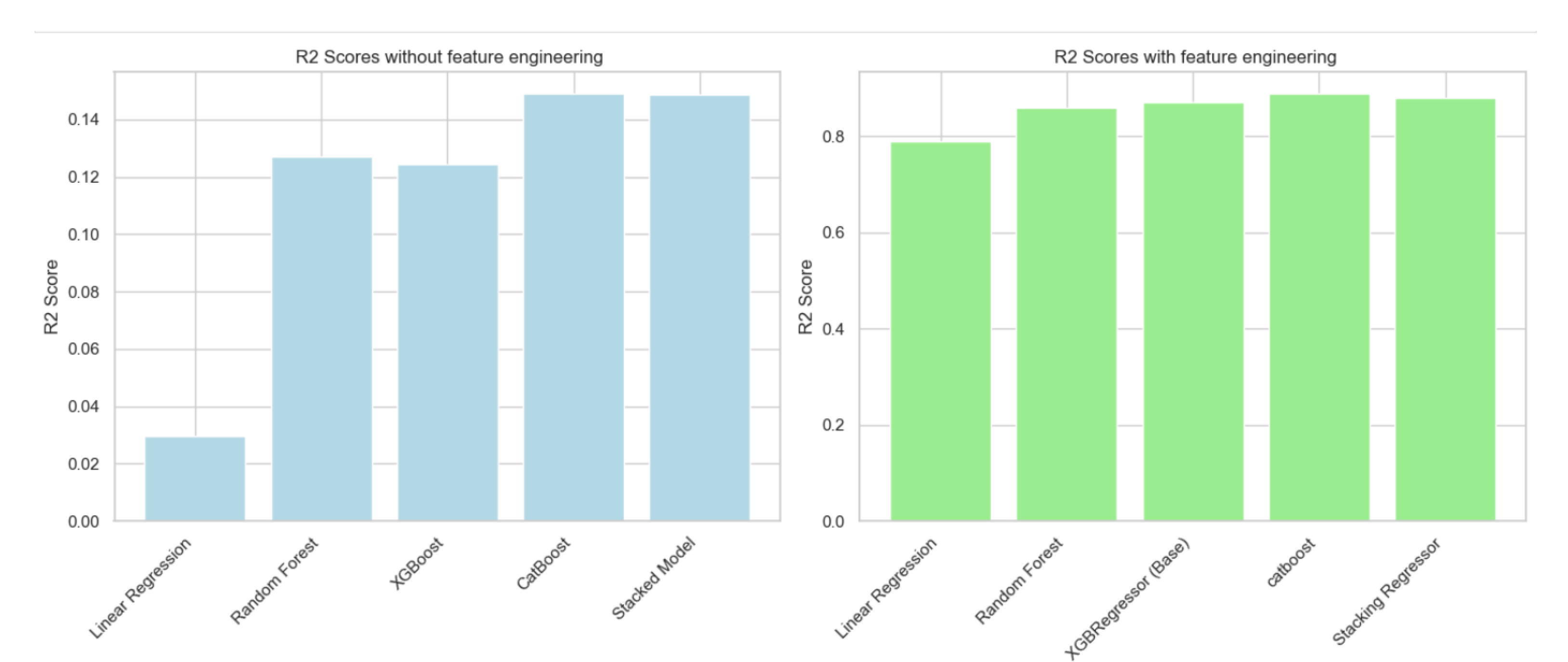
Figure 2.
Process flow diagram. Note that just to optimize the space usage, we have placed the names of some ML algorithms on the left, right and bottom, but they do not have any special meaning based on their position in the diagram.
Figure 2.
Process flow diagram. Note that just to optimize the space usage, we have placed the names of some ML algorithms on the left, right and bottom, but they do not have any special meaning based on their position in the diagram.
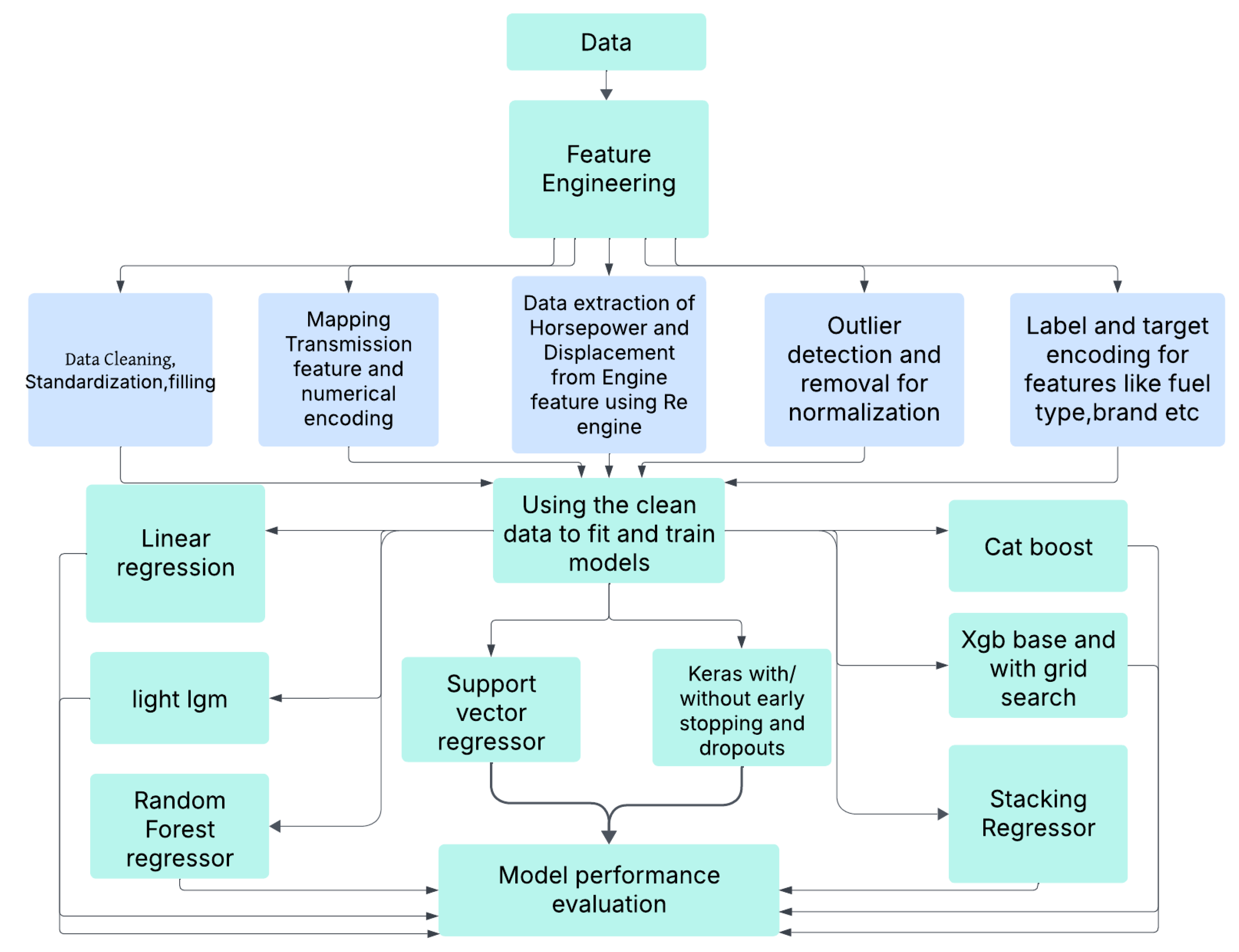
Figure 6.
Car distribution in the dataset by brand. A few manufacturers dominate, resulting in a long-tail distribution.
Figure 6.
Car distribution in the dataset by brand. A few manufacturers dominate, resulting in a long-tail distribution.

Figure 7.
Feature importance plot showing the influence of each variable on model predictions.

Figure 8.
Comparison of scores before and after feature engineering across selected models. Performance improved dramatically for all models, especially for ensemble-based regressors.
Figure 8.
Comparison of scores before and after feature engineering across selected models. Performance improved dramatically for all models, especially for ensemble-based regressors.

Figure 10.
Comparison of different regression models based on and RMSE scores.

Figure 11.
Execution Time Comparison (in seconds) for Different Regressors, highlighting the trade-off between model complexity and training duration.
Figure 11.
Execution Time Comparison (in seconds) for Different Regressors, highlighting the trade-off between model complexity and training duration.
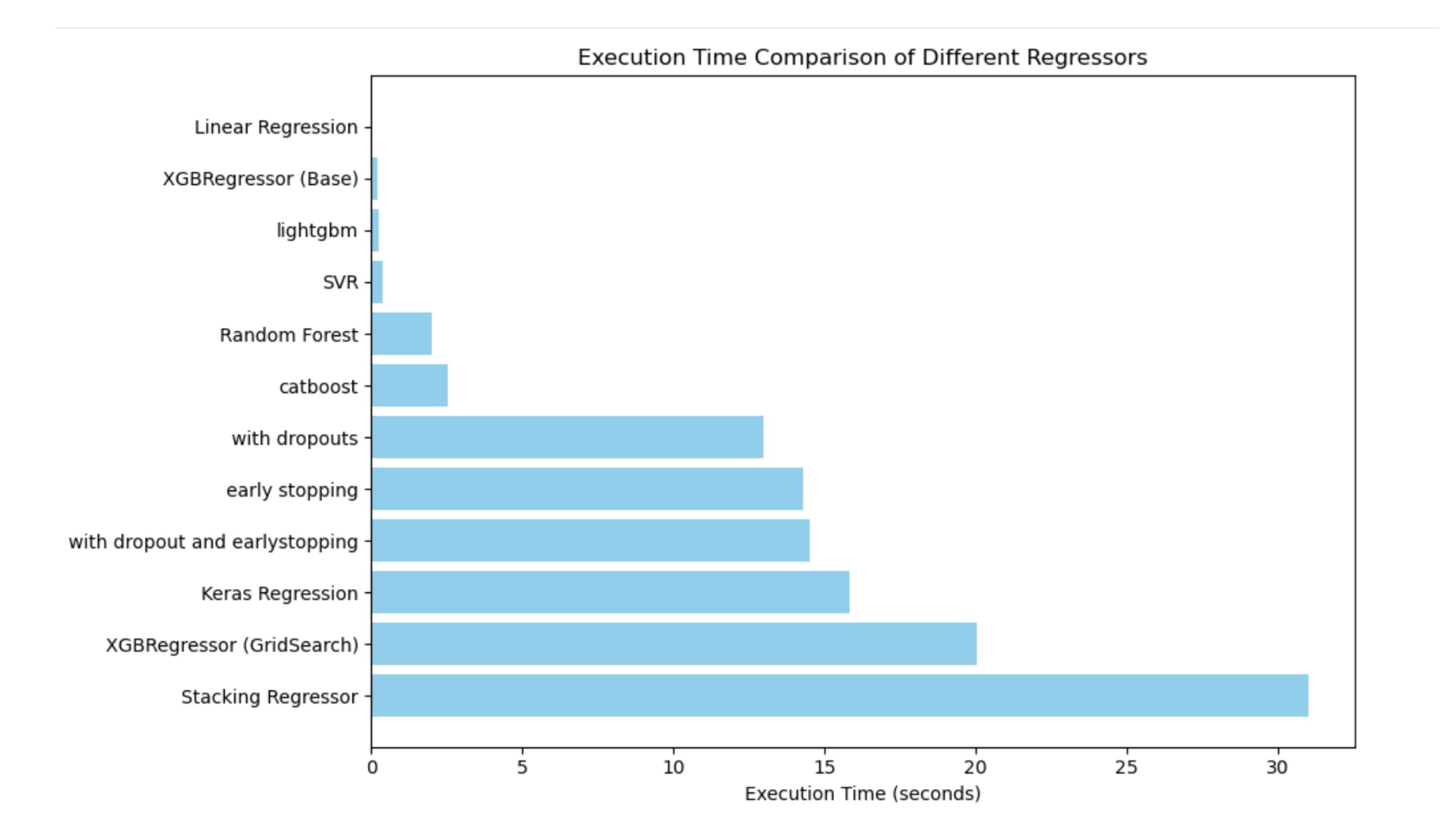
Figure 12.
Model Performance Comparison Before and After Feature Engineering. While ensemble models performed reasonably well even on unprocessed data, all models, especially Linear Regression, saw substantial gains following structured preprocessing. RMSE is shown on a log scale to visualize both high and low error magnitudes.

Figure 13.
Improvement in R2 Score Due to Feature Engineering. Linear Regression experienced the largest absolute gain, while all models showed substantial improvements, reinforcing the importance of structured preprocessing.
Figure 13.
Improvement in R2 Score Due to Feature Engineering. Linear Regression experienced the largest absolute gain, while all models showed substantial improvements, reinforcing the importance of structured preprocessing.

Figure 14.
Reduction in RMSE After Feature Engineering. All selected models showed a significant decrease in prediction error, particularly Linear Regression, which benefited the most from improved feature quality.
Figure 14.
Reduction in RMSE After Feature Engineering. All selected models showed a significant decrease in prediction error, particularly Linear Regression, which benefited the most from improved feature quality.
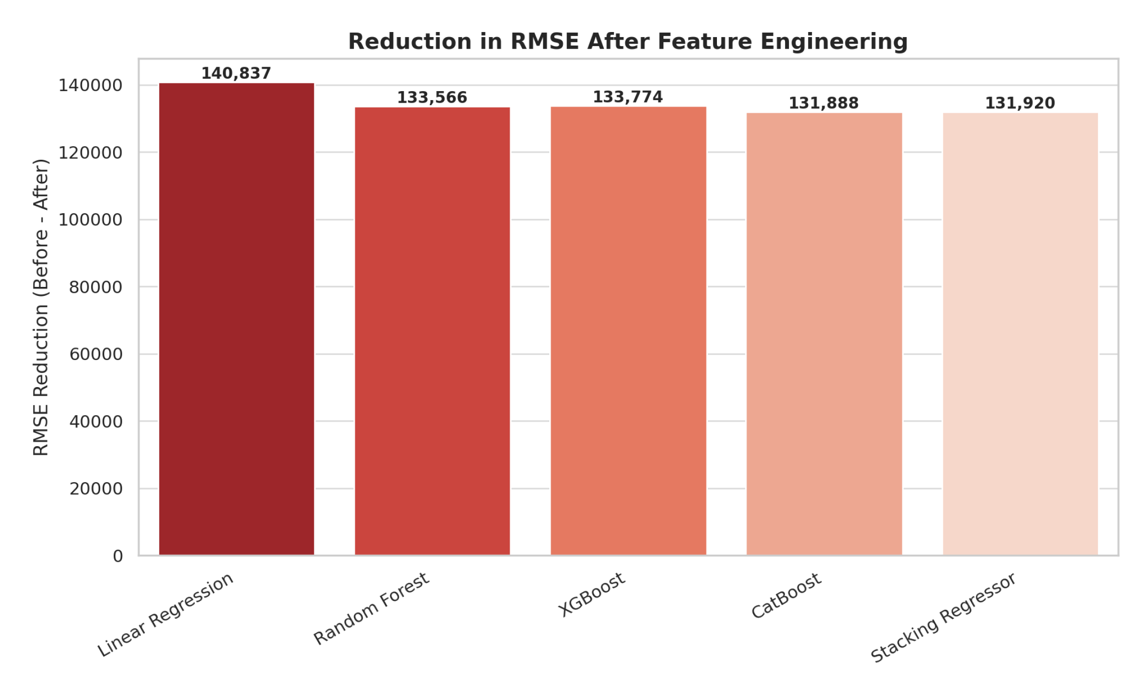
Table 2.
Comparison of R² Scores and RMSE for Different Regression Models.
| Regressor | RMSE | R² Score |
|---|---|---|
| Stacking Regressor | 0.1208 | 0.8899 |
| CatBoost | 0.1216 | 0.8890 |
| XGBoost (Grid Search) | 0.1213 | 0.8888 |
| LightGBM | 0.1225 | 0.8840 |
| XGBoost Regressor | 0.1262 | 0.8798 |
| Random Forest | 0.1313 | 0.8697 |
| SVR | 0.1447 | 0.8419 |
| Neural Network (Keras) | 0.1602 | 0.8061 |
| Linear Regression | 0.1634 | 0.7983 |
| Neural Network (Dropout & Early Stopping) | 0.2950 | 0.3429 |
Table 3.
Comparison of R² Scores and RMSE Before and After Feature Engineering for Selected Models.
| Model | R² Score (Before) | R² Score (After) | RMSE (Before) | RMSE (After) |
|---|---|---|---|---|
| Linear Regression | 0.0296 | 0.7983 | 140838.13 | 0.1634 |
| Random Forest | 0.1272 | 0.8697 | 133566.21 | 0.1313 |
| XGBRegressor (Base) | 0.1245 | 0.8798 | 133774.73 | 0.1262 |
| CatBoost | 0.1490 | 0.8890 | 131888.52 | 0.1216 |
| Stacking Regressor | 0.1486 | 0.8899 | 131920.13 | 0.1208 |
Disclaimer/Publisher’s Note: The statements, opinions and data contained in all publications are solely those of the individual author(s) and contributor(s) and not of MDPI and/or the editor(s). MDPI and/or the editor(s) disclaim responsibility for any injury to people or property resulting from any ideas, methods, instructions or products referred to in the content. |
© 2025 by the authors. Licensee MDPI, Basel, Switzerland. This article is an open access article distributed under the terms and conditions of the Creative Commons Attribution (CC BY) license (http://creativecommons.org/licenses/by/4.0/).
Copyright: This open access article is published under a Creative Commons CC BY 4.0 license, which permit the free download, distribution, and reuse, provided that the author and preprint are cited in any reuse.


