
Submitted:
10 July 2025
Posted:
15 July 2025
You are already at the latest version
Abstract
Assessment of the quality of sports motion is very important for providing individual training and adapting to current performance. In handball, a good shooting motion is key during a match. In this study, a method is proposed to automatically classify expert and beginner handball shooting motions. This method is illustrated using the public H3DD dataset. This dataset contains the motions of 44 beginners and 18 experts. Each shooting action is represented by a sequence of 3D skeletons. The proposed method uses a dynamic time-warping algorithm, with three angles extracted from each frame. These three angles were selected by expert handball coaches as representatives of the shooting motion dynamics in each frame. This is the first time that handball player ability has been automatically classified during a shooting motion using the aforementioned public dataset. The proposed method achieved an average accuracy of 90.47% for the test set (10% test, 90% training) by using randomly selected balanced samples from the dataset.
Keywords:
pattern recognition
; signal processing
; artificial intelligence
; images
; motion analysis
; dynamic time warping
; skeleton
; performance evaluation
; sports
; handball
1. Introduction
Artificial intelligence has been increasingly used in the analysis, learning, and recognition of sports motion. Sensors used to acquire motion data can be attached to the human body or operated remotely.
The sensors most commonly used include color cameras to generate image sequences, inertial measurement units (IMU) to provide information on kinematics, including acceleration, rotation, direction, and angular velocity; range sensors to measure depth; pressure sensors to measure force per unit area; electromyographic sensors to quantify muscle contraction intensity; heart rate sensors to monitor heart activity; and geolocation sensors to provide latitude, longitude, and elevation [1].
Human motion can be described by using physical models. For instance, kinematics helps to describe linear and angular motions. Kinetics are related to the causes of motion such as forces, torque, and moments. Work, energy, and power help sports science quantify the efficiency and calories spent [1].
To describe and understand human actions using the data provided by sensors, signals must be processed to derive high-level knowledge. Machine learning and pattern recognition play key roles in data transformation [1-3].
Human activity recognition (HAR) can be categorized as simple or complex. [4] proposed four levels of human activity: gestures, actions, interactions, and group activities. Gestures are simple movements of a person´s body. These actions are single-person activities. Interactions involve two or more people and objects. Group activities are performed by conceptual groups of multiple people and/or objects.
For HAR in sports, [3] proposed three main categories: individual, joint, and team activities. Individual actions occur when only one player is involved in the action to be recognized. Joint activities involve at least two players performing a combination of one or more simple actions, interactions with objects and/or complex actions. Finally, team activities are strategic actions involving the entire team.
Owing to the proliferation of depth cameras and methods for accurately estimating the joint locations of the human body, skeleton representations are widely used for human activity recognition [5]. The public dataset H3DD used in this study uses skeleton sequences to represent individual actions [6].
A vitally important skill in handball is shooting. It allows you to score and pass. At its most basic, shooting is an overarm shot, and there are many variations. It is also basic to develop players’ initiative to threaten goals and to identify when there is a good opportunity to score. In this context it is fundamental to learn how to throw correctly [22]. Given the importance of overarm shots in handball, they are the subject of research of this paper, using the H3DD dataset [6,20].
The rest of the introduction section will present related works to handball activity recognition, then a summary of the contributions, and finally the organization of the rest of the paper.
The papers described in the following are related to handball activity recognition (Figure 1). The sensors most used in activity recognition and motion analysis in handball include color (Red,Green,Blue) RGB or (Depth) RGB-D cameras, IMUs, and local positioning systems (LPS) [3], [6], [7].
Machine learning approaches in handball movement analysis use handcrafted or deep features [3], [8]. [9] reviewed different methods for 3D pose estimation and tracking using a sequence of images captured from a monocular camera. They assessed 12 methods of 3D pose estimation using a custom dataset of handball jump shots. Most methods which were developed in other sports and scenarios exhibit performance degradation in unseen scenarios, such as handball actions.
[11] presented a method for detecting and tracking handball players in videos.They used manual and automated extracted blobs to train a boosting algorithm. Their method achieved 84% accuracy in detecting players in the same game in a test set, and 74% accuracy in an unseen game. For a 3 min video with a single player, the percentage of frames automatically tracked with boosting tracking was 84%.
[12] performed multiple tracking of handball players. They used a combination of player detection at each frame using YOLOv3 and then determined the optimal tracking of each player using the DeepSort algorithm.
[13] showed how to use IMUs and local positioning systems (LPS) to monitor the positions and activities of handball players in a match to determine physical demands. Other researchers have focused on biomechanical analysis of motion [7], [14].
[7] tested 17 experienced handball players to automatically measure ball velocity and classified different approaches (jump, running, standing) and throw types (circle, whip) using IMUs and machine learning. The authors used a random forest classifier. The ball’s velocity was predicted with an error of 1.05 m/s. The average accuracy for classifying approach types varied between 88% and 95%, and for throw types was 85 – 95%.
[14] investigated 11 joint movements during overarm throwing in experienced handball players. They found that elbow angle and internal rotation velocity of the shoulder at ball release were strongly correlated with throwing performance. Additionally, better throwers started to rotate their pelvis earlier during throwing.
Finally, the studies mostly related to activity recognition in handball are [8], [10], [15], [16]. [8] developed a method for building a dataset for action recognition learning in handball. Sections of the video showing the beginning of an action were manually selected. Then, the players were automatically detected using the Mask R-CNN. Players were tracked using activity measures derived from optic flow computations. Tracking of the related bounding boxes in successive frames was performed by applying the Hungarian algorithm. This method was tested for four actions: passing, dribbling, shooting, and jump-shot.
[10] created semi-manually the UNIRI-HBD_v2 dataset for handball action recognition. This dataset contains nine action classes (crossing, shot, defense, jump shot, dribbling, throw, catch, running, and passing). The authors compared several deep learning models for player and ball detection, player tracking, concatenating frames, validation of action sequences, action recognition, and spatiotemporal localization. They found that existing models are reliable for person detection but not for ball detection. Specialized models must be developed to detect the ball. General object tracking and pedestrian tracking models did not perform well on this specialized dataset. For action recognition, the best recognition result was F1=78%, which was averaged over all the classes.
[15] use the position and tracking of team players from a plan view to generate temporal segmentation and recognition of team activities in sports. They illustrated their method in handball and field hockey. Their method computed the position distribution for each frame. From these distributions, five motion images were computed through frame differencing and optic flow. Subsequently, six features were computed for each motion image using second-order weighted moments. The concatenation of these features using frames before and after proved useful for classifying activities using a support vector machine classifier. Their method achieved a 94.61% correct classification rate (CCR) for six handball activities and 88.06% CCR for eight field hockey activities.
[16] presented several strategies for determining the most active players in handball. Their proposal includes detection, tracking, and activity measures.
It is very interesting that, through other considerations, [6] found very similar angles to [14] as features for the comparison of throwing motion. In their work, [6] used shoulder angle, elbow angle, and trunk inclination. They determined these angles based on advice from experienced coaches and analysts and by selecting the angles at the joints that had higher interclass correlation coefficients.
In the present study, the same angles chosen by [6] were used as features to automatically classify the performance during the overarm thrown motion.
The main contributions of this study are as follows: 1. This is the first time a method has been presented to automatically classify overarm shots in handball for experts or beginners. 2. This method is illustrated using the public H3DD dataset of overarm shots, which includes the movements performed by experts and beginners. Our method is a novel combination of existing techniques for feature extraction and normalization in sequences of 3D skeletons before using existing classifiers. 3. Because the H3DD dataset is unbalanced in terms of the number of elements for experts and beginners and includes shots performed by left-handed and right-handed people, the method describes preprocessing for handling both situations. We are using traditional sampling methods to deal with unbalanced sets. Our method describes how to handle the data from left-handed and right-handed people to extract features in a uniform way in both cases. 4. It is shown that by extracting balanced samples from the dataset, classification accuracy increases. 5. A comparison is made in classification between using directly the distance provided by dynamic time warping (DTW), and a K-NN classifier, and using features obtained with the warped trajectories. The warping path provided by dynamic time warping allows us to select a normalized number of frames to extract feature vectors for each motion sequence. It is shown that by using these features, better classification results are obtained. The description of the features obtained from the warped trajectories is described in more detail in section of Materials and Methods.
The remainder of this paper is organized as follows. Section 2 describes the public dataset H3DD used for the experiments as well as the proposed method for automatically classifying overarm shots between expert and beginner levels. Section 3 Experiments and Results presents the experiments performed with the public dataset, the results and evaluation of the proposed method. Section 4 discusses the results in the context of existing literature. Finally, Section 5 provides conclusions, limitations, and perspectives for future work.
2. Materials and Methods
This section describes the main characteristics of the public H3DD dataset of handball overarm throwing motion [6,20] as well as the method proposed for learning and automatically classifying the throw ability of experts and beginners.
2.1. H3DD Dataset of Handball Overarm Throws
The H3DD dataset of handball overarm throws was first introduced in [6], and is available at [20]. The handball players that generated the dataset included 18 experts and 44 beginners. Each player performs a single shot. Therefore, the dataset consists of 18+44= 62 overarm throws. Because the throws are divided into two different folders for expert and beginner throws, they are implicitly labelled with their class ability. The expert and beginner level of each player is determined by the original creators of the database. They were advised by an expert handball coach. One important aspect that was not highlighted in the original paper [6] that introduced the dataset is that some players were left-handed, and others were right-handed. This information was not explicitly available in the dataset; therefore, we labeled each throw with this information.
Each player’s throw was recorded using an MS Kinect V2 sensor while shooting the handball goal. The details of the experimental scenario and acquisition protocol can be found in [6].
The MS Kinect V2 sensor can track up to six people and generate five streams [17]: 1) RGB sequence of images, 2) depth sequence of images, 3) 2D sequence of skeletons, 4) 3D sequence of skeletons, and 5) audio streams.
For each overarm throw in the H3DD dataset only the 3D sequence of skeletons is available. In each frame, the human body is represented by a 3D skeleton, which is a graphical representation consisting of 25 3D joints connected by 24 segments. Each 3D joint consists of 3D coordinates in meters (x=horizontal, y=vertical, z=depth) with respect to the MS Kinect V2 coordinate system.
The number of frames for each throw in the H3DD dataset varied. For the expert throws, the dataset had seven frames for each throw. For beginners, the dataset varied between six and 22 frames. The characteristics of the dataset are summarized in Table 1.
2.2. Hardware and Software
The experiments and results described in this paper were obtained using a laptop with 16 GB RAM, 11th Gen Intel Core i7-1165G7 @ 2.80 GHz, 1.69 GHz (base), 256 GB SSD, running Windows 10 Pro 22H2, 64 bits.
The software used was MATLAB R2024a 64 bits.
2.3. Method
To automatically learn and classify the throws in the H3DD dataset from the 3D skeleton sequences into expert and beginner classes, it is worth highlighting three sources of variability in the dataset (Table 1). 1) Different dominant arms for performing the throw (right- or left-handed), 2) the numbers of frames in each throw for the beginner class can vary between 6 and 22 frames, and 3) unbalanced classification classes. There were more examples of beginner throws than of expert throws (44/18= 2.44 times).
The proposed method considers the above-mentioned sources of variability in the H3DD dataset as follows: 1) Because the features that are used to learn and classify the throwing motion depend heavily on the arm that performs the action (left or right), the dataset was augmented with this label information; thus, the method can select the appropriate 3D joints to extract features. This additional information does not affect the purpose of the method, which automatically classifies the ability and not the identification of the throw laterality (left or right). 2) As in [6], we use the dynamic time warping (DTW) algorithm [18] to obtain invariance to the speed of realization of the movement because the number of frames varies with each throw. The beginners’ sequences were processed to obtain normalized uniform sequences of length 7 frames. We chose this number of frames, as this is also used for all the expert sequences. 3) When extracting examples from the unbalanced dataset for training and testing, random sampling was performed to obtain balanced sets. Further details of these procedures are provided below. The main steps of the proposed method are illustrated in Figure 2.
2.4. Features
[6] analyzed all the angles and their Interclass Correlation Coefficient (ICC) in the joints and skeleton generated by MS Kinect V2 for two classes of beginner and expert handball players, and found that the trunk inclination angle, shoulder angle, and elbow angle were more useful (informative) than the remaining angles. These angles were proposed as features to characterize the overarm-throwing motion (Figure 3). [14] through kinematic analysis of the overarm throwing motion in experienced handball players, found that the elbow angle and shoulder angle showed a strong relationship with performance.
The handball coach at our university also confirmed that the angles proposed by [6] are good discriminators for analyzing overarm throwing motion, and these are the angles that we used in this research as features to classify overarm throwing motion between expert and beginner players.
To calculate these three angles from the skeleton and 3D joints generated by the MS Kinect V2, some of these joints were used to define two vectors for computing each angle, as shown (Figure 3).
The trunk inclination angle α1 was measured by the angle between vectors U1 and V1. Vector U1 moves from the hip joint to the shoulder joint. Vector V1 moves from the hip joint to the knee joint (Figure 3). For shoulder angle α2, the angle between vectors U2 and V2 was used. Vector U2 moves from the shoulder joint to the spine-shoulder joint. Vector V2 moves from the shoulder joint to the elbow joint (Figure 3). Finally, the elbow joint angle α3 was computed from the vectors U3 and V3. U3 moved from the elbow joint to the shoulder joint and V3 connected the elbow joint to the wrist joint (Figure 3). It is important to note that to use a specific joint provided by the MS Kinect V2 sensor, it is necessary to indicate the side of the body that is performing the motion, that is, the throw in this case. For example, if the player is left-handed, to compute vector U1, the left hip and left shoulder joints are used. This observation highlights the importance of determining the dominant arm during throwing motion.
The three angles, αi, i = 1,…,3, are computed using the formula to obtain the angle between two vectors (1).
An overarm throwing motion is represented by three angles αi, i = 1,…,3, for each frame.
2.5. Uniform Sequence Length and Alignment
Because some overarm throws are fast or slow, it is important to obtain invariance in the speed of realization to analyze the configuration of the body from the beginning to the end of the motion.
The dynamic time warping (DTW) algorithm allows the comparison of similarities and differences between signals with different time durations [18]. In addition, it provides correspondence between the parts of the two signals through the “warping path.”
In the case of overarm throw sequences, for each frame, we take three angles αi, i = 1,...,3 for each sequence (1). If sequence X is composed of M samples (frames) each in three-dimensional space (K=3), and if sequence Y is composed of N samples (frames) in 3D space (K=3), then both signals can be represented by matrices. Sequence X is a K × M matrix (2) and sequence Y is a K × N matrix (3).
Given d(X(m),Y(n)), the distance between the mth sample of X and the nth sample of Y specified by a metric, the DTW algorithm stretches signals X and Y onto a common set of instances such that the global signal-to-signal measure is the smallest [18].
The DTW algorithm seeks a path parameterized by two sequences of the same length, ix and iy, such that d* is minimum (4) [18].
In addition, the DTW algorithm provides the common set of instants ix, iy or “warping path,” such that X(ix) and Y(iy) have the smallest possible distance d*, between them [18].
The vectors ix, iy each contain a monotonically increasing sequence in which the indices of the elements of the corresponding signal, X or Y, are repeated the necessary number of times [18].
Some overarm-throwings in the dataset H3DD are composed of different numbers of frames (Table 1). Using the three angles, αi, i = 1,..,3, for each frame and concatenating them to obtain a feature vector for a sequence, results in feature vectors of different lengths.
Using the warping path provided by DTW, it is possible to align two sequences to obtain sequences of the same length. However, when creating the H3DD dataset, [6] manually performed frame sampling for all expert throws to leave each expert sequence of length seven frames (Table 1). In contrast, beginner sequences varied in length; apparently, they did not apply the same manual procedure (Table 1).
To normalize all beginner sequences to seven frames, we applied the following procedure: Of the 44 beginner sequences (Table 1), there were five sequences in the H3DD dataset that had seven frames. From these five sequences, we obtain an initial beginner model, iteration = 0, inspired by the expert model procedure described in [6]. The initial beginner model, iteration=0, was obtained by computing the median of each angle αi, i = 1,...,3, for all frames in the sequence. For example, for computing the median of angle αi, for a fixed angle “i", and fixed frame, we compute the median using the values of that angle coming from the five beginners’ sequences for the fixed frame.
That is, if α_mbijk, i = 1,...,3, j=1,..7, k=0, is the value of the initial beginner model for angle i, frame j, iteration k=0, and is computed for each angle i, each frame j, and iteration k fixed as
Where the angles α_ij (fixed i, and j) come from the five beginner sequences that have 7 frames (iteration k=0).
With this initial beginner model, α_mbijk, i = 1,...,3, j=1,..7, k=0, all beginner sequences can be normalized to seven frames using the DTW algorithm and the warping path ix, iy provided.
Now that we have transformed the beginner sequences into seven frames, the beginner model α_mbijk, i = 1,...,3, j=1,..7, k=1, is updated for iteration k=1 using (5). However, all 44 transformed beginner sequences are now used.
With the beginner model α_mbijk, i = 1,...,3, j=1,..7, k=1, at this iteration involving all 44 transformed beginner sequences, using the DTW algorithm, and the warping paths ix, iy, 44 transformed beginner sequences were obtained from seven frames each.
Although the process could continue iterating, at this step, we stopped, now that we have 44 transformed beginners’ sequences each of seven frames.
After this normalization process, all transformed sequences have seven frames each. The expert sequences were not transformed because they already had 7 frames each. Now, all transformed sequences can be represented by three angles per frame, with seven frames each, α_ij, i = 1,...,3, j=1,..7. By concatenating all the features (three angles per frame), a sequence (seven frames) can now be represented by 3 × 7 = 21 features.
It is now possible to perform a classification process; however, because the classes are unbalanced (18 expert sequences and 44 beginner sequences) (Table 1), in the next section, we describe a sampling process to obtain balanced classes.
2.6. Balanced Classes
The sampling process used to obtain a dataset with balanced classes is very simple. Because there are 18 expert sequences and 44 transformed beginner sequences, the sampling process without repetition, randomly extracted 18 sequences from the transformed 44 beginner sequences.
Then, every time the random sampling process is completed, a dataset of 18 expert and 18 beginner sequences is obtained. The extracted balanced dataset is then used for the classification process. We apply a cross-validation procedure for training and validation with five folds but always setting apart a percentage of data for testing, that is not involved in the training, validation process. More details are provided in the next section, and in the experiments section.
2.7. Classification
For the classification process, a dataset consisting of 18 experts and 18 randomly selected beginner throws was prepared. For each throw sequence, the features are 3 × 7 =21 (three features per frame, seven frames), and the dataset for classification is represented by a matrix of 36 rows (18 expert and 18 beginner throws) and 22 columns (21 features per throw, plus an indicator variable, 0 for beginner and 1 for expert throw).
We followed a cross-validation procedure for training and validation, and a percentage of the dataset is set apart for testing and does not participate in training and validation. For the cross-validation process during training and validation five folds were used.
The experiments and results of applying 34 classifiers are described in the next section. These are the classifiers that are part of the MATLAB interactive classification application [19].
The 34 classifiers used for testing in the experiments are listed in Table 2.
3. Experiments and Results
For the experiments, since there were 2.44=44/18 more beginners than expert shots, a random sampling without repetition of beginners’ shots was performed 10 times to obtain balanced datasets of 18 experts and 18 beginners.
For each dataset, 34 classifiers were tested, and in each case, portions of 10%, 20%, and 30% were left aside in the dataset for the classification test [19]. In other words, a separate set is set aside that is not involved in training or validation. The results of the classification experiments using the different test sets are summarized in Table 3. It is important to mention that the partitions routine from Matlab works randomly, and divides the dataset in training, validation and test subset, in integer values, and as closest as possible to the specified values (e.g. 10%, 20%, or 30% for the test subsets). The number of elements in each subset is always integer.
Table 3 shows the metrics of the best classifier (number 20) after averaging each classifier separately with the randomly balanced dataset selected for the classification. In this case, we generated ten balanced datasets extracted randomly from the H3DD unbalanced dataset. The partition of the dataset in training-validation and testing is represented by the notation TV (train-validation)/T(testing); for instance, 70/30 means that 70% of the dataset was used for training and validation and 30% for testing.
The performance metrics of accuracy, precision, recall, specificity, F1 and true negative rate (TNR) can be computed from Equations (6) – (11).
where TP, FN, TN, and FP are the true positive, false negative, true negative, and false positive, respectively.
4. Discussion
In [6], where the H3DD dataset was introduced, the authors used the DTW distance for several purposes, but not for automatically classifying expert and beginner shots. They used the DTW distance for the following interesting applications: 1) to measure the distance of beginners from a static model of experts to rank the beginners; 2) to measure the distance of beginners from a dynamic model of experts to rank the beginners; 3) for each beginner, rank the experts according to the DTW distance for the static case, using only one frame; and 4) for each beginner, rank the experts using DTW distance to match for individual training, for the dynamic case, using all the frames.
In complement to [6], the DTW distance can be used for classification. It is important to clarify that [6] did not do an automatic classification procedure. In this paper we do automatic classification of expert and beginners’ sequences.
We tried to directly use the DTW distance for classification in combination with the KNN algorithm for various values of K and folds, using the unbalanced dataset, and then the balanced dataset. However, these results were lower than those obtained using the method proposed in this study. A comparison of these scenarios is shown in Table 4 for the best case of K=4 and Folds=5. The comparable partition was 80/20 with 80% for training and 20% for testing. The metrics used were precision (7), recall (8), accuracy (6), and F1 (10).
As can be seen from the comparison results (Table 4), the balanced classes procedure in the dataset and the sequence normalization through the warping path of DTW generate a constant-size feature vector for the dynamic sequences, allowing the use of off-the-shelf classifiers. The increment of the F1 metric following the proposed procedure was 34.08% = 77.41%–43.33%, compared with using the DTW distance and KNN classifier directly without any normalization.
It is important to note that the proposed method provides higher accuracy when more data is used for training, such as in the 90/10 scenario (90% for training and 10% for testing), which provides an average accuracy of 90.47% (Table 3).
5. Conclusions
This paper presented a method for automatically learning and classifying overarm throw shots in expert and beginner handball classes.
This method was applied to the public dataset H3DD of handball shots, which were manually labelled in experts and beginners. This dataset has some particularities, because some of the shots were performed by right-handed players and others by left-handed players. The number of members in each class was different, generating unbalanced classes, and the number of frames per sequence varied (Table 1). This is the first time that the automatic classification of handball shots has been reported for the H3DD dataset.
For the case of 80% training and validation, and 20% testing, our method achieved F1 = 77.41%, which is 34.08% higher than that of a direct application of the DTW distance and a classification method such as KNN (Table 2). For the case of 90% training and validation, and 10% testing, our method increases its average F1 metric to 87.50% (Table 2).
The proposed method can be adapted for comparing and classifying other movements in handball and other sports provided in terms of skeleton sequences (Fig. 1).
One limitation of the proposed method is that the number of reference frames used to normalize each class through the warping path is not automatically determined. For the H3DD dataset of the expert class, the sequences were already normalized in seven frames; therefore, this number of frames was a natural choice for normalizing the beginners’ class (Table 1).
Future work will study how to automatically determine the number of frames for each class, and when the number of classification classes is greater than two. For instance, if the classification ability is graded as beginner, intermediate, or expert, or if it is graded using a categorical representation [0,1, 2…, 10] or a continuum scale (for example, grading ability as 8.5).
Author Contributions
“Conceptualization, H.V.R.F., M.L.A.G., and J.J.C.G. ; methodology, H.V.R.F., M.L.A.G.; software, H.V.R.F.; validation, H.V.R.F., M.L.A.G., and J.J.C.G..; formal analysis, H.V.R.F., M.L.A.G., A.M.H., J.J.C.G. investigation, H.V.R.F., M.L.A.G.; resources, H.V.R.F.; data curation, H.V.R.F.; writing—original draft preparation, H.V.R.F.; writing—review and editing, H.V.R.F., M.L.A.G., A.M.H., J.J.C.G.; visualization, H.V.R.F.; supervision, H.V.R.F.; project administration, H.V.R.F..; funding acquisition, H.V.R.F. All authors have read and agreed to the published version of the manuscript.”.
Funding
“This research received no external funding”.
Data Availability Statement
The dataset used in this research was introduced in [6], and is available at: https://github.com/Elaoud/H3DD-dataset.git.
Conflicts of Interest
“The authors declare no conflicts of interest.”.
References
- Ashley, K. Applied machine learning for health and fitness; Apress: Berkeley, CA, USA, 2020. [Google Scholar]
- Bishop, C.M. Pattern recognition and machine learning; Springer: New York, NY, USA, 2006. [Google Scholar]
- Host, K.; Ivasic-Kos, M. An overview of human action recognition in sports based on computer vision. Heliyon 2022, 8(6), E09633. [Google Scholar] [CrossRef] [PubMed]
- Aggarwal, J.K.; Ryoo, M.S, Human activity analysis: a review. ACM Computing Surveys 2011, 43 (3) 16 1-43.
- Lo Presti, L.; La Cascia, M. 3D skeleton-based human action classification: A survey. Pattern Recognition 2016, 53 130-147.
- Elaoud, A.; Barhoumi, W.; Zagrouba ,E., et al. Skeleton-based comparison of throwing motion for handball players. J Ambient Intell Human Comput 2020,11 (4) 419-431.
- Van den Tillaar, R.; Bhandurge, S.; Stewart, T. Detection of different throw types and ball velocity with IMUs and machine learning in team handball. In ISBS Proceedings Archive, Liverpool, U.K. 2020.
- Pobar, M.;. Ivasic-Kos, M. Mask R-CNN and Optical Flow Based Method for Detection and Marking of Handball Actions. In 11th International Congress on Image and Signal Processing, BioMedical Engineering and Informatics, Beijing, China, 13-15 October 2018.
- Sajina, R.; Ivasic-Kos, M. 3D pose estimation and tracking in handball actions using a monocular camera. J Imaging 2022, 8(11), 308. [Google Scholar] [CrossRef] [PubMed]
- Host, K.; Pobar, M.; Ivasic-Kos, M. Analysis of Movement and Activities of Handball Players Using Deep Neural Networks. J Imaging 2023, 9(4), 80. [Google Scholar] [CrossRef] [PubMed]
- Barros, R. M. L.; Menezes, R. P.; Russomanno, T. G. : et al. Measuring handball players trajectories using an automatically trained boosting algorithm. Comput Methods Biomech Biomed Engin 2010, 14(1), 53–63. [Google Scholar] [CrossRef] [PubMed]
- Host, K.; Ivasic-Kos,M.; Pobar, M. Tracking Handball Players with the DeepSORT Algorithm. In 9th International Conference on Pattern Recognition Applications and Methods, Valletta, Malta, 22-24 February 2020.
- Lefevre, T.; Guignard, B.; Karcher, C.; et al. A deep dive into the use of local positioning system in professional handball: Automatic detection of players' orientation, position and game phases to analyze specific physical demands. Plos One 2023, 18(8), e0289752. [Google Scholar] [CrossRef] [PubMed]
- Van den Tillaar; R.; Ettema G. A three-dimensional analysis of overarm throwing in experienced handball players. Journal of Applied Biomechanics 2007, 23 (1) 12-19.
- Direkoǧlu, C.; O’Connor N.E. Temporal segmentation and recognition of team activities in sports. Machine Vision and Applictions 2018, 29 (3) 891-913.
- Pobar, M.; Ivasic-Kos, M. Active player detection in handball scenes based on activity measures. Sensors 2020, 20 (5) 1475.
- Mathworks. Key Features and Differences in the Kinect V2 Support.
- https://la.mathworks.com/help/imaq/key-features-and-differences-in-the-kinect-v2-support.html (accesed on 10 12 2024).
- Mathworks. DTW. Distance between signals using dynamic time warping.
- https://la.mathworks.com/help/signal/ref/dtw.html?lang=en accesed on 10 12 2024).
- Mathworks. Classification learner App. https://la.mathworks.com/help/stats/classification-learner app.html?lang=en.
- (accesed on 10 12 2024).
- Elaud, A. 2018. H3DD dataset of experts and beginners handball shots. https://github.com/Elaoud/H3DD-dataset.
- Murphy, K.P. 2022. Probabilistic Machine Learning. MIT Press, Cambridge, Massachusetts, USA.
- Hapkova, I.; Estriga, L.; Rot, C. 2019. Teaching handball, Volume 1: Teacher Guidelines, Handball at School, fun, passion and health. International Handball Federation, Basel, Switzerland.
Figure 1.
Main categories in related works to activity recognition in handball.
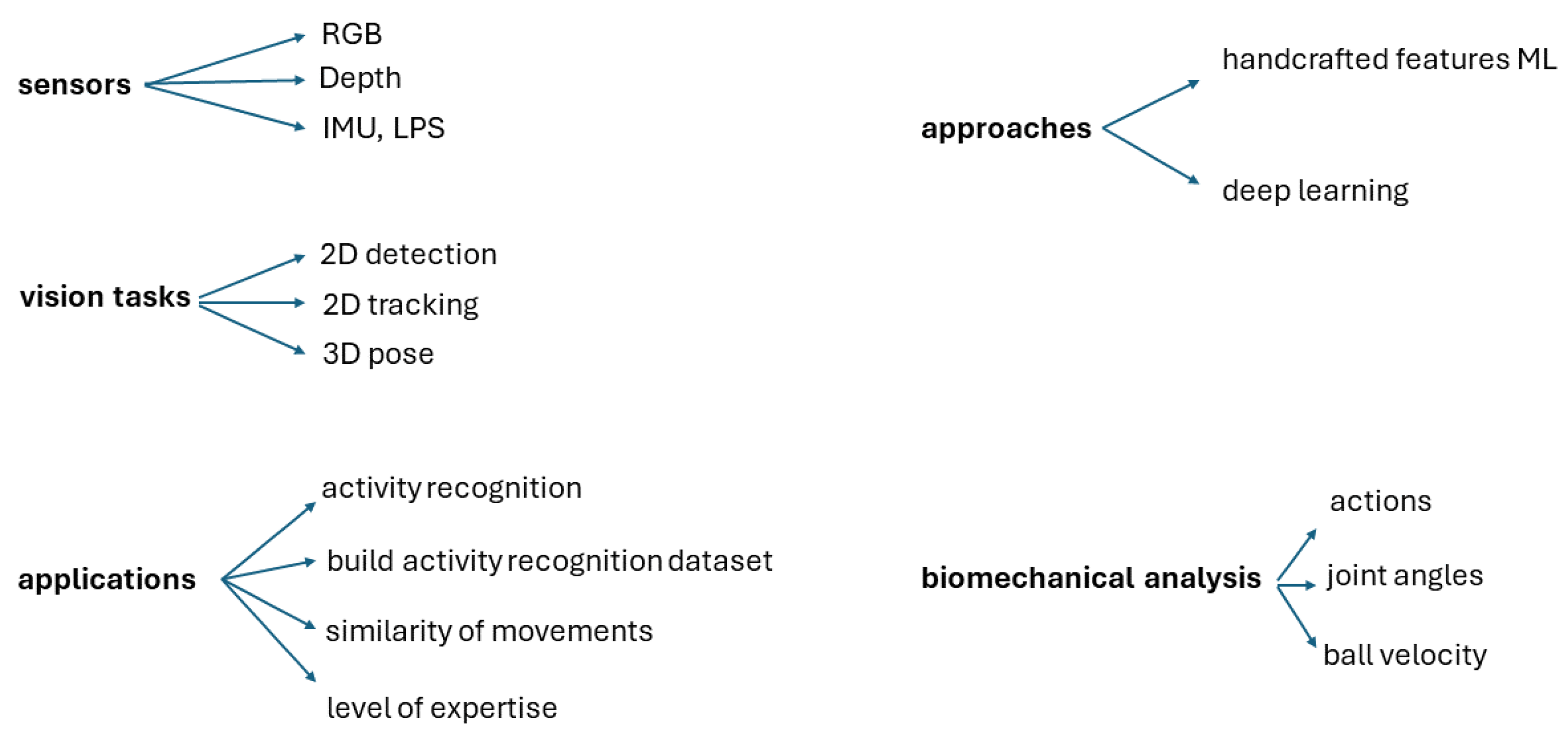
Figure 2.
Main steps for the proposed method for automatically learning and classifying handball overarm throws in expert or beginner classes.
Figure 2.
Main steps for the proposed method for automatically learning and classifying handball overarm throws in expert or beginner classes.
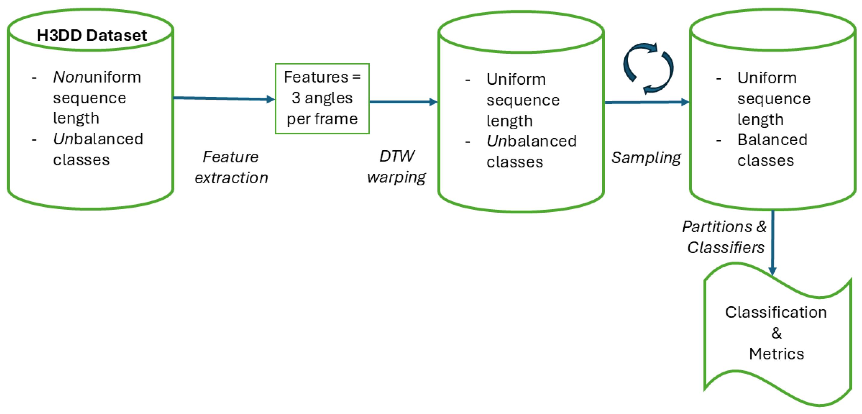
Figure 3.
Main Skeleton and 25 3D joints generated by MS Kinect V2 along with the three angles (α1,α2,α3) proposed by [6] to characterize overarm throwing motion.
Figure 3.
Main Skeleton and 25 3D joints generated by MS Kinect V2 along with the three angles (α1,α2,α3) proposed by [6] to characterize overarm throwing motion.
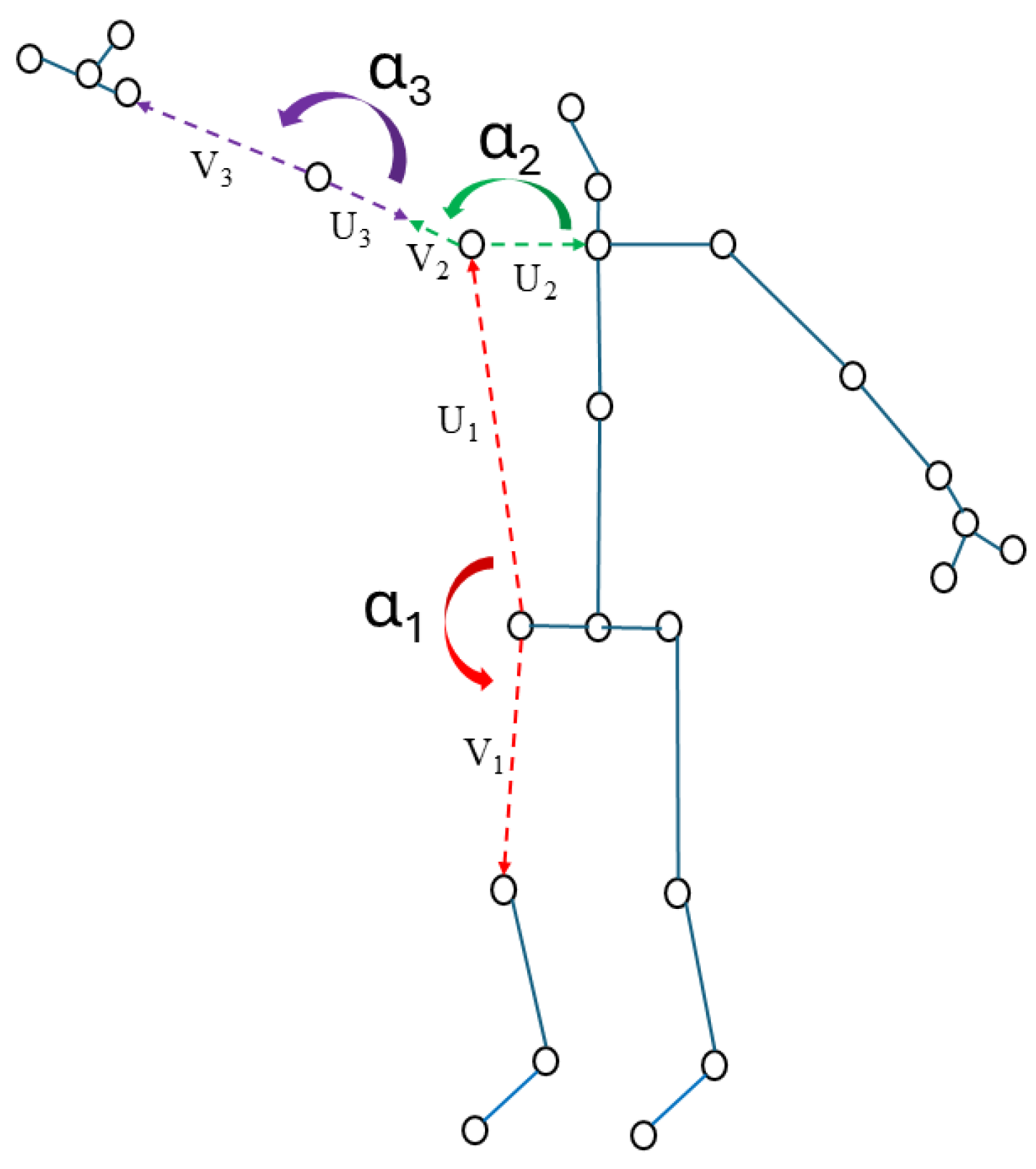

Table 1.
H3DD Dataset Composition.
| Characteristic | Expert | Beginner |
| Right-handed | 14 | 37 |
| Left-handed | 4 | 7 |
| Total | 18 | 44 |
| Frames range | 7 | 6 - 22 |
Table 2.
Classifiers used in the experiments.
| Model Number | Model Type | Hyperparameters |
| 1 | Tree | Maximum number of splits: 100; Split criterion: Gini's diversity index; Surrogate decision splits: Off |
| 2 | Tree | Maximum number of splits: 20; Split criterion: Gini's diversity index; Surrogate decision splits: Off |
| 3 | Tree | Maximum number of splits: 4; Split criterion: Gini's diversity index; Surrogate decision splits: Off |
| 4 | Linear Discriminant | Covariance structure: Full |
| 5 | Quadratic Discriminant | Covariance structure: Full |
| 6 | Binary GLM Logistic Regression | None |
| 7 | Efficient Logistic Regression | Learner: Logistic regression; Solver: Auto; Regularization: Auto; Regularization strength (Lambda): Auto; Relative coefficient tolerance (Beta tolerance): 0.0001; Multiclass coding: One-vs-One |
| 8 | Efficient Linear SVM | Learner: SVM; Solver: Auto; Regularization: Auto; Regularization strength (Lambda): Auto; Relative coefficient tolerance (Beta tolerance): 0.0001; Multiclass coding: One-vs-One |
| 9 | Naive Bayes | Distribution name for numeric predictors: Gaussian; Distribution name for categorical predictors: Not Applicable |
| 10 | Naive Bayes | Distribution name for numeric predictors: Kernel; Distribution name for categorical predictors: Not Applicable; Kernel type: Gaussian; Support: Unbounded; Standardize data: Yes |
| 11 | SVM | Kernel function: Linear; Kernel scale: Automatic; Box constraint level: 1; Multiclass coding: One-vs-One; Standardize data: Yes |
| 12 | SVM | Kernel function: Quadratic; Kernel scale: Automatic; Box constraint level: 1; Multiclass coding: One-vs-One; Standardize data: Yes |
| 13 | SVM | Kernel function: Cubic; Kernel scale: Automatic; Box constraint level: 1; Multiclass coding: One-vs-One; Standardize data: Yes |
| 14 | SVM | Kernel function: Gaussian; Kernel scale: 1.1; Box constraint level: 1; Multiclass coding: One-vs-One; Standardize data: Yes |
| 15 | SVM | Kernel function: Gaussian; Kernel scale: 4.6; Box constraint level: 1; Multiclass coding: One-vs-One; Standardize data: Yes |
| 16 | SVM | Kernel function: Gaussian; Kernel scale: 18; Box constraint level: 1; Multiclass coding: One-vs-One; Standardize data: Yes |
| 17 | KNN | Number of neighbors: 1; Distance metric: Euclidean; Distance weight: Equal; Standardize data: Yes |
| 18 | KNN | Number of neighbors: 10; Distance metric: Euclidean; Distance weight: Equal; Standardize data: Yes |
| 19 | KNN | Number of neighbors: 100; Distance metric: Euclidean; Distance weight: Equal; Standardize data: Yes |
| 20 | KNN | Number of neighbors: 10; Distance metric: Cosine; Distance weight: Equal; Standardize data: Yes |
| 21 | KNN | Number of neighbors: 10; Distance metric: Minkowski (cubic); Distance weight: Equal; Standardize data: Yes |
| 22 | KNN | Number of neighbors: 10; Distance metric: Euclidean; Distance weight: Squared inverse; Standardize data: Yes |
| 23 | Ensemble | Ensemble method: AdaBoost; Learner type: Decision tree; Maximum number of splits: 20; Number of learners: 30; Learning rate: 0.1; Number of predictors to sample: Select All |
| 24 | Ensemble | Ensemble method: Bag; Learner type: Decision tree; Maximum number of splits: 25; Number of learners: 30; Number of predictors to sample: Select All |
| 25 | Ensemble | Ensemble method: Subspace; Learner type: Discriminant; Number of learners: 30; Subspace dimension: 11 |
| 26 | Ensemble | Ensemble method: Subspace; Learner type: Nearest neighbors; Number of learners: 30; Subspace dimension: 11 |
| 27 | Ensemble | Ensemble method: RUSBoost; Learner type: Decision tree; Maximum number of splits: 20; Number of learners: 30; Learning rate: 0.1; Number of predictors to sample: Select All |
| 28 | Neural Network | Number of fully connected layers: 1; First layer size: 10; Activation: ReLU; Iteration limit: 1000; Regularization strength (Lambda): 0; Standardize data: Yes |
| 29 | Neural Network | Number of fully connected layers: 1; First layer size: 25; Activation: ReLU; Iteration limit: 1000; Regularization strength (Lambda): 0; Standardize data: Yes |
| 30 | Neural Network | Number of fully connected layers: 1; First layer size: 100; Activation: ReLU; Iteration limit: 1000; Regularization strength (Lambda): 0; Standardize data: Yes |
| 31 | Neural Network | Number of fully connected layers: 2; First layer size: 10; Second layer size: 10; Activation: ReLU; Iteration limit: 1000; Regularization strength (Lambda): 0; Standardize data: Yes |
| 32 | Neural Network | Number of fully connected layers: 3; First layer size: 10; Second layer size: 10; Third layer size: 10; Activation: ReLU; Iteration limit: 1000; Regularization strength (Lambda): 0; Standardize data: Yes |
| 33 | Kernel | Learner: SVM; Number of expansion dimensions: Auto; Regularization strength (Lambda): Auto; Kernel scale: Auto; Multiclass coding: One-vs-One; Standardize data: Yes; Iteration limit: 1000 |
| 34 | Kernel | Learner: Logistic Regression; Number of expansion dimensions: Auto; Regularization strength (Lambda): Auto; Kernel scale: Auto; Multiclass coding: One-vs-One; Standardize data: Yes; Iteration limit: 1000 |
Table 3.
Classification results of the best classifier (Classifier number 20).
| Train/test rate | Accuracy | Precision | Recall | F1 | TNR |
| 70/30 | 72.85 | 76.66 | 65.71 | 70.76 | 80.00 |
| 80/20 | 76.66 | 85.71 | 70.58 | 77.41 | 84.61 |
| 90/10 | 90.47 | 87.50 | 87.50 | 87.50 | 92.30 |
Table 4.
Methods comparison.
| Method | Precision | Recall | Accuracy | F1 |
| KNN unbalanced Dataset | 37.71 | 58.67 | 57.44 | 43.33 |
| KNN balanced Dataset | 55.73 | 82.95 | 56.95 | 65.75 |
| Proposed Method | 85.71 | 70.58 | 76.66 | 77.41 |
Disclaimer/Publisher’s Note: The statements, opinions and data contained in all publications are solely those of the individual author(s) and contributor(s) and not of MDPI and/or the editor(s). MDPI and/or the editor(s) disclaim responsibility for any injury to people or property resulting from any ideas, methods, instructions or products referred to in the content. |
© 2025 by the authors. Licensee MDPI, Basel, Switzerland. This article is an open access article distributed under the terms and conditions of the Creative Commons Attribution (CC BY) license (http://creativecommons.org/licenses/by/4.0/).
Copyright: This open access article is published under a Creative Commons CC BY 4.0 license, which permit the free download, distribution, and reuse, provided that the author and preprint are cited in any reuse.


