Submitted:
09 July 2025
Posted:
11 July 2025
You are already at the latest version
Abstract
Doppler scatterometers have demonstrated the ability to measure wide-swath ocean surface currents from airborne platforms. Since platform velocities for spaceborne platforms are almost two orders of magnitude larger, errors in the knowledge of the pointing of the radar antenna result in ocean current errors also two orders of magnitude larger, and this presents a major challenge to achieving useful measurements of ocean currents. Here, we present a new calibration method to estimate pointing biases that allows the removal of the dominant pointing errors and allowing the retrieval of global ocean currents with modest requirements on the system stability. The calibration method can be implemented in ground processing and does not impact the processing of onboard data. We illustrate the performance of the calibration on the performance of the proposed NASA/CNES ODYSEA Doppler scatterometer and assess its ability to meet the mission science goals.
Keywords:
ocean currents
; doppler scatterometry
; spaceborne
1. Introduction
Doppler scatterometers [1] are rotating pencil-beam radars that can be used for wide-swath simultaneous estimation of surface currents and winds. Although lower resolution than along-track interferometers [2], they can estimate wide-swath vector surface currents and winds by combining measurements of Doppler shift and backscatter cross sections along different look directions. This architectural difference makes them ideal candidates for global surface winds and currents mission [3] capable of acquiring daily synoptic global maps of surface winds and currents, which have many applications. Recently, NASA has selected the ODYSEA mission concept [3,4,5,6,7], which uses a Doppler scatterometer as its main instrument, for phase-A development as part of the first Earth Explorer set of mission concepts, and it is expected to make a decision regarding proceeding to the next phase in 2026.
Doppler scatterometer instruments have been demonstrated successfully from airborne platforms. Most recently, the Sub-Mesoscale Ocean Dynamics Experiment (S-MODE) [8], a NASA Earth-Ventures Suborbital (EVS3) mission, demonstrated to capability of airborne Doppler scatterometers to measure surface currents [9] and winds [10] with results that compare favorably against traditional in situ observations (e.g., ADCPs, anemometers). Scaling the airborne design to a spaceborne setting requires additional transmit power and a larger antenna [4], well within current technical capabilities, to achieve similar precision as that obtained from airborne instruments, albeit at lower spatial resolution. However, to achieve similar accuracy, the systematic error due to the need to know the antenna pointing accurately must be addressed, and that is the objective of this paper.
Translating radial surface velocities into currents requires knowledge of pointing vector. In [1], it is shown that an error in knowledge of , the azimuth angle between the platform velocity vector and the antenna look vector, results in an error of the ground-projected radial surface velocity, , given by , where is the platform speed. The different impact between air and spaceborne platforms due to is due to the vastly different platform speeds between the two cases. As an example, to achieve an accuracy greater than 10 cm/s (a threshold for the ODYSEA mission), requires a pointing knowledge of rad for an airborne instrument ( m/s), while requiring rad for a spaceborne instrument ( km/s), or nearly two orders of magnitude greater knowledge. For the spaceborne case, present Inertial Motion Units (IMUs) are capable of estimating pointing drifts with greater precision over short times ( minute), but suffer from drifts that will exceed the desired accuracy over much longer times. Similarly, mounting an antenna or controlling its long-term pointing drift due to thermoelastic low-frequency disturbances is beyond current direct measurement capabilities.
To overcome these challenges in the airborne case, Rodríguez et al. [1] acquired flight lines in opposite directions to separate the effects of pointing and ocean motion. Clearly, this cannot be done with a spaceborne instrument. A similar issue with pointing knowledge arises in wide-swath interferometric altimeters [11], such as the NASA/CNES SWOT mission, and a calibration approach based on the difference of scales between the ocean signal and the measurement errors, as well as the use of satellite cross-overs, has been demonstrated [12,13]. The typical time between cross-overs is greater than one hour, and often can be on the order of days. For SWOT, this works due to a very rigid, and expensive, mechanical system which results in very slow drifts for most of the orbit. Here, we explore an alternate approach that has the potential to work for much faster (shorter than one orbit period) drifts.
They key to our proposed approach is the fact that, for the very large swaths typical of spaceborne Doppler scatterometers, the ocean current signal has a spatial signature very different from the errors induced by pointing. This separation becomes evident when the radial velocity signatures are averaged along-track, and one of the key questions addressed in this paper is how long these averaging times must be in order to reduce leakage from the ocean current signature.
The details of the proposed algorithm are presented in Section 2.1, where we see that the leakage of ocean currents constitutes the main driver for the required averaging times. Section 2.2 discusses the sources of random errors for while Section 2.3 describes the simulation we use to assess the limitations of the calibration scheme. In Section 2.4, we examine the potential use of various sources of a priori ocean circulation information to mitigate current leakage and reduce the required averaging time. Section 3 presents the results of the simulation of the calibration scheme for a realistic orbit scenario, and the implications of these results for the design of future Doppler scatterometer missions is discussed in Section 4.
2. Materials and Methods
2.1. Calibration Approach
Following [1], we model the measured surface-projected radial velocity in the presence of an azimuth knowledge error, , as
where t labels the measurement time, or, equivalently, the along-track position; is the pointing error we seek to calibrate; and n represents random measurement errors. We only consider errors in azimuth pointing, since, as shown in [1], the elevation angle can be estimated from the radar timing to much greater accuracy than required here.
We separate into errors which vary quickly ( min), and cannot be calibrated using the approach proposed here, and slowly varying systematic errors ( min), which are our target. Quickly varying errors may be due to residual spin rate changes not captured by the antenna spin encoder; fast oscillations of the antenna structure (e.g., due to thermal snaps at a terminator crossing); or fast mechanical pointing changes not captured by the sensor IMU. We assume these errors can be minimized by adding suitable sensors (IMUs, azimuth angle encoders) to the instrument, by placing suitable requirements on the spacecraft and antenna mechanical structures, or adding them to the random error n.
The slowly varying errors may be due to thermoelastic deformation of the antenna or spacecraft not captured by pre-launch models or masked due to IMU drift; or they could be due to residual errors in the spin encoder sensor, which may fail to capture thermally driven changes in the antenna spin uncaptured by the encoder. The first kind of error will introduce time-varying shifts of the pointing, so that is uncorrelated with , and the radial velocity error will be proportional to . The second kind of errors, which have been observed in the DopplerScatt instrument [1], will induce errors which are periodic in , and may also vary slowly in time. The effect of an order m harmonic error in will be to introduce harmonic errors in due to the multiplication of by in .
The idea in our proposed algorithm is to use the fact that, over long wavelengths, the ocean circulation is uncorrelated with , whereas both of the systematic error sources have signatures which are periodic in . The first step in the algorithm is to bin into bins and estimate the average radial velocity as a function of . The minimum amount of time needed to perform the binning is given by the antenna rotation period, sec for ODYSEA.
In the absence of surface currents, this binning would be sufficient to produce a calibration of . However, as we will see below, if uncompensated, ocean motion may introduce significant errors in the estimates of . One way to reduce this leakage is to average along-track so that ocean features average out. The spatial scale of ocean currents and the platform velocity set the required averaging times. For most of the oceans, mesoscale eddies (diameter km) contribute much of the ocean leakage. Given typical spacecraft velocities, this would imply that the averaging time would need to be on the order of minute. There are, however, very long wavelength circulation patterns, such as western boundary currents (e.g., the Gulf Stream) or equatorial circulation, have significantly longer wavelengths and may produce geographically localized leakage if the averaging time is too short.
A potential way to mitigate for ocean currents is to use the fact that, at large scales, ocean circulation can be estimated independently by existing sensors (e.g., altimeters and scatterometers), or represented with sufficient skill by operational ocean circulation models. We can sample these prior models to the same space-times as the radar observations and produce , the prior estimate of the ocean circulation, which we can then subtract from the radial velocity observations to reduce the leakage from ocean motion. Section 2.4 discusses possible priors that could be used in the timeframe of the ODYSEA mission.
If we denote by the operation of binning observations by followed by along-track averaging for a time T, the following equations summarize the estimation algorithm for
where is the estimator for the pointing error correction; the first term on the right-hand side is the desired result; the second term represents the residual ocean leakage (after potentially removing a prior estimate of ocean motion); and the last term is the residual random error. We perform the temporal averaging by using a sliding, uniformly-weighted window of time-duration T, and associate with it a time t at the center of the window. It is possible that the averages may contain data over land or ice, and these data are discarded, so that the data in the moving window does not always contain the same number of samples, or may be missing altogether if insufficient data are present to form the averages.
2.2. Pointing Error Characteristics
The calibration model introduced above can accommodate any set of distortions that dependent on the azimuth angles and vary slowly enough so that ocean leakage and random errors can be averaged out. The model is not parametric and can accommodate arbitrary pointing characteristics that satisfy these requirements. Some errors considered here (e.g., thermoelastic distortions) are amenable to parametric modeling given a mechanical design, and the accuracy of the models at the microradian level may be hard to achieve or validate. While such models will undoubtedly help to improve pointing calibration, our goal here is more conservative: we examine the feasibility of using a generic model, with limited parametrization, that can accommodate a wide variety of feasible pointing error distortions.
Since is periodic, the most generic model for that satisfies these requirements can be written as
where N is the number of azimuth bins. Environmental parameters, such as variations in solar radiation along the orbit, will determine the specific form of the temporal variation of the harmonic coefficients. Without making any parametric assumptions about this variability, we assume that, for short enough periods compared to the characteristic times of drivers of the distortion, the temporal variability of the systematic pointing error can be modeled as a first order autoregressive (AR1) process, namely:
where is a zero-mean Gaussian variable, and is the update time between azimuth binning. This will result in a random process that has an exponential correlation time given by . The variance of is related to the total variance of by . Due to the linearity of the Fourier transform, , , will also be AR1 processes with correlation time . However, there is freedom to choose their contribution to the total variance, as long as the sum of the variances adds to the total variance. Below, we will investigate the effects of distributing the error between different harmonics; i.e., high- or low-frequency dominant errors.
It is instructive to examine the effect of different harmonics in the expansion on the surface current errors. Following [1], the radial velocity error can be translated into errors in the along-track, , and cross-track, , surface current components, and the results for the ODYSEA swath are shown in Figure 1. It is clear that the spatial frequency of the velocity errors increases with harmonic order. For low order harmonics, the errors will induce errors across the swath that are clearly unphysical and might be corrected using basin-scale circulation models. Higher harmonics will start to mimic mesoscale signatures and may have greater impact on meeting science goals. The ODYSEA mission [6,7], for instance, can meet most of its science goals by filtering out longer wavelengths (e.g., by applying a Gaussian filter whose width is 130 km) and concentrating on the residual mesoscale signals. In Figure 1, we show the residual errors after applying such a filter: lower-order harmonics have almost no contribution to the mesoscale errors.
It should be noted that, while we use the time-varying harmonic expansion to characterize the physical impact of different errors, and their relationship to sources in the hardware, the calibration algorithm introduced in the previous section does not estimate the harmonic expansion coefficients. Rather, it estimates , the net correction that must be applied to the radial velocity, independent of its source. The estimation of the harmonic expansion coefficients is not required for radial velocity correction, although it may be informative for understanding the error sources, and suffers additional estimation errors.
2.3. Data Simulator
We have built a global measurement simulator to assess the feasibility of the pointing calibration. The simulator uses two weeks of the ODYSEA orbit and generates space and time locations over the radar footprint for each antenna pointing location, radar range, and Doppler scatterometer pulse-pair. These data were then averaged over each radar footprint and pulse burst to generate an average radial velocity for each burst location. This is similar to the process that would be implemented during processing of the data as inputs to the calibration algorithm. The angular extent of the burst footprint is small enough that no useful information is lost, given the angular resolution of the azimuth binning used, which utilizes 1024 bins.
Two global ocean simulations were used to feed the ODYSEA simulator. The first is an uncoupled ocean simulation, and the second is a coupled ocean-atmosphere simulation. The reasoning is that the uncoupled simulation has a spacing grid resolution of ∼2 km, which permits the generation of a more vigorous small-scale ocean motions. Whereas the coupled simulation produces a more vigorous internal gravity wave continuum and wind-driven currents not well resolve in the uncoupled simulation.
The global high-resolution LLC-4320 (Latitude-Longitude-polar Cap 4320) model dataset features a horizontal spacing grid resolution of 1/48° and includes 90 vertical levels. The vertical resolution varies from 0.5 m at the sea surface ad 480 m at the seafloor. The model is forced by the European Centre for Medium-range Weather Forecasts (ECMWF) Atmospheric Reanalysis data, with a resolution of and updated every 6 hours. A more detailed description of the model can be found in Torres et al. [14].
The COAS (Coupled Ocean Atmosphere Simulation) model consists of the GEOS atmospheric and land model coupled to an ocean configuration of the MITgcm. GEOS was configured to run with a nominal horizontal grid spacing of 6.9 km and 72 vertical levels, while the MITgcm was configured to run with a nominal horizontal grid spacing of (up to 4.6 km at the equator) and 90 vertical levels. Both models are integrated and coupled every 45 s. Model outputs contain hourly three-dimensional atmospheric fields, and many diagnostic variables. A detailed description of COAS can be found in Torres et al. [6]. Further details of the GEOS configuration can be found in Molod et al. [15] and Strobach et al. [16], while MITgcm setup is described in Arbic et al. [17].
2.4. Ocean Prior Data
We consider ocean prior datasets that either simulate satellite measurement capabilities currently available, or use global data acquired by the Doppler scatterometer itself.
To simulate current satellite capabilities, we generated datasets that mimic the AVISO [18] and OSCAR [19] global products. The AVISO product uses altimeter measurements from multiple platforms to generate a global estimate of geostrophic currents. These currents do not contain ageostrophic components, such as wind-driven Ekman currents. The OSCAR product aims to add these wind driven currents by using winds from multiple scatterometer instruments, together with a simple model for the wind-driven currents. We follow a standard procedure to generate the satellite-like products by filtering the reference simulation (either LLC-4320 or COAS) in space and time. The AVISO-like (or geostrophic) dataset was generated by applying a 3-day running mean filter and 60 km diameter Gaussian spatial filter to the sea surface height. Afterwards, the geostrophic surface currents are computed, excluding the equatorial band, where geostrophy does not apply. To mimic OSCAR products, we analyzed OSCAR real-time Level 4 dataset provided by PO.DAAC (https://doi.org/10.5067/OSCAR-25N20). The analysis consisted of computing a frequency-wavenumber spectrum to determine the scales of variation resolved by OSCAR. The surface currents from COAS were low-passed with a 4-day running mean and 60 km diameter Gaussian filter. Figure 2 shows sample spectra for the OSCAR product used in our analysis, and the OSCAR-like and geostrophic products obtained by filtering the COAS simulation. Notice the close agreement between the OSCAR and OSCAR-like products and the reduced energy for the geostrophic currents.
Aside from priors derived from other satellites, it is possible to use the Doppler scatterometer data itself to generate ocean priors. One of the limitations of the OSCAR data is that the wind measurements are not collected at the same time as the surface currents. In addition, the wind-driven surface currents are parametrized as due to Ekman currents alone. Using the COAS model as truth, we derive an empirical wind-driven current by starting with the winds and currents estimated by the Doppler scatterometer, subtract a geostrophic current from the AVISO-like product (where available), compute the along and across-wind components of the residual currents, and average the results conditioned by wind speed. Since the response of the currents to winds will have a latitudinal dependence (see [19]), the globe is divided into 5-degree latitude bins and a separate estimate is obtained for each bin. Once the averages of the along and across-wind current components are obtained, one can estimate the wind speed dependence of the wind-driven current magnitude and direction relative to the wind. We find that a linear fit with wind speed is a good approximation to the data. Figure 3 shows the values for the constant, , and wind-speed proportionality coefficient, , for the magnitude and direction of the wind-driven currents. Away from the tropics, there is a negligible term for the current magnitude, while there will be a current whose magnitude is approximately 1% of the wind speed and which will be rotated approximately relative to the wind direction (depending on hemisphere). These results are qualitatively similar to Ekman currents. In the tropics, on the other hand, there is a stronger mean current along the wind direction, and stronger dependence on wind speed. This is not unexpected when geostrophy does not apply. Given these model fits, we construct a prior model for the wind driven current by fitting a smooth spline through the data, as shown in Figure 3. This wind driven current prior can then be used by itself, or in conjunction with an AVISO-like estimate of the geostrophic currents.
As a final ocean prior model, we consider the current climatology obtained by averaging the Doppler scatterometer data over a period of time (two weeks, in our case). Averaging the Doppler scatterometer data will average out, to some extent, the pointing errors when their correlation time is much shorter than the time over which the current "climatology" is constructed. The resulting climatology will only be weakly correlated with the instantaneous pointing errors, but will represent well the long wavelength, low frequency ocean circulation.
To assess the geographic variability of the prior, we present in Figure 4 the global mean and standard deviation of the residual radial velocities. After subtracting the geostrophic currents, the residuals are only reduced at mid-latitudes, but equatorial and Southern Ocean currents, where ageostrophy dominates, are not well represented. The empirical Ekman and combined geostrophic and Ekman do much better in reducing the residuals in these regions, but significant residuals can still be seen in the tropics, where the simple empirical model has only limited skill, and in the Southern Ocean, where transient strong wind events are not well captured by a static model. Next in skill is the two-week climatology, which, since it uses actual observations, does a better job at capturing equatorial circulation. However, a two-week climatology still misses strong transient wind events. Finally, the most skillful prior is the OSCAR-like product which does the best at capturing equatorial currents and transients. There is a concern, however, that, since the simulated data was produced from the true model by simple space-time averaging, it may have more dynamics skill that the current generation of OSCAR products have, but may represent model skill when ODYSEA is deployed.
3. Results
In this section, we use the characteristics of the Doppler scatterometer in the ODYSEA mission [3,4,5,6,7] as an example to assess the performance of the calibration algorithm in a realistic scenario. The ODYSEA instrument uses a conical scanning beam with a rotation period of 6 seconds to map a 1500 km swath that achieves 90% global mapping every day. The mission goals require a total threshold total error of 50 cm/s at 5 km resolution, which can then be averaged to km scales to achieve mapping of the ocean mesoscale [20,21]. The radial velocity pointing error, which is long-wavelength and systematic, is allocated a maximum threshold error of 7 cm/s, which is the driver for the required along-track averaging time. The current velocity errors grow near the nadir and outer swaths [1], so vector current mapping meeting the full requirements uses data from two subswaths symmetric around the nadir (called the vector swaths), while achieving the mission space-time and accuracy goals requires even smaller subswaths (called the performance swaths) the centered around azimuth angles of 45 deg. Below, we examine the impact of residual pointing errors over both subswaths.
3.1. Ocean Leakage
Residual ocean currents present the largest challenge to our pointing algorithm. As shown in Figure 4, this leakage can be significant, even after subtracting ocean priors and can preset long-wavelength signatures. We average along-track to reduce this leakage and present in Figure 5 the global residual errors for radial velocity and the two surface velocity components.
It is clear from this Figure that, without a prior correction or with the geostrophic correction, meeting the measurement requirement will require significant averaging: on the order of 20 minutes or, equivalently, of latitude. Using the Ekman priors or the two-week climatology will reduce the required averaging time by one-half, while the OSCAR-like prior will reduce it by about one-quarter. These time scales set the scales for the stability of the pointing system error stability. Pointing errors which vary more quickly must be measured directly or assimilated into the total measurement error budget.
Examining Figure 4 shows that the residuals will have signatures dominated by longer wavelengths, consistent with the red power-law spectrum for ocean circulation. From Figure 1, we see that longer ocean wavelengths correspond to the longer period harmonics of the pointing error, so it is reasonable to assume that ocean leakage will affect mostly the estimates of the low-frequency pointing errors. To quantify this, we perform a Fourier decomposition of the ocean leakage term, which is periodic in , and present the results for no priors, geostrophic + Ekman priors, and OSCAR-like priors in Figure 6.
As with the ocean current, the leakage spectrum follows a red spectral power-law, with the first few harmonics dominating most of the variability. The impact of the prior data is to reduce the low-frequency leakage, while the higher frequencies are similar in all cases.
To gauge the relative impact of the random measurement errors against the leakage, we also plot the random measurement error spectrum. In all cases, it is orders of magnitude smaller than the ocean leakage up to about 100 cycles, given the minimum averaging time of 10 minutes discussed above.
This dominance of the low-frequency harmonics has important implications on setting the pointing knowledge or control. In Figure 7, we plot the residual leakage if it can be assumed that the error induced by a varying number of low order harmonics can be neglected. These harmonics control very long wavelength errors, as shown in Figure 1, and may not affect the science that can be achieved when studying the mesoscales. The figure shows that the total knowledge requirements can be achieved with substantially shorter averaging times, and that for the cases where a prior is available, the measurement requirements can be met if the first couple of harmonics can be neglected or controlled mechanically. These harmonics are introduced mainly by thermoelastic distortions of the spacecraft, where a suitable mechanical model can be developed prior and after launch.
We expect the satellite to encounter similar environmental conditions from one orbit to another. Therefore, we investigate an additional approach based on the averaging between consecutive orbits. It aims at controlling the errors induced by thermoelastic effects, as well as the previous harmonic approach.
To do so, we average each time window (from 1 to 100 minutes) with the corresponding time windows of a given number of consecutive orbits. In fact, it consists of a sliding average centered on the current orbit (in the same way as the temporal averaging). We then plot the resulting ocean leakage of radial velocity in Figure 8.
Figure 8 illustrates the decrease of ocean leakage with the averaging among more and more orbits. It shows that this method enables to reduce the averaging time needed to meet the requirement, and therefore keep a good resolution of thermoelastic distorsions.
On the one hand without the use of a prior (left), we ensure that the 1 orbit average (blue line) shows consistent results with regards to Figure 5. Moreover, a 30 orbits average (purple line) enables to reduce required temporal average to 5 minutes.
On the other hand, the use of a prior (right) shows significant improvements, as a 10 orbits window (less than a day) is enough to meet the requirement without a temporal average any longer than 1 minute. It should be noted that the mean current prior we consider is the mean of 1.5 year COAS model interpolated on ODYSEA groundtrack. As it is already quite a conservative prior, we could expect to reduce leakage even more with the use of seasonal means.
3.2. Time Varying Errors
In addition to the ocean surface current leakage, the temporal variability of the pointing error is the other major constraint on the length of the along-track averaging time. To minimize the error, averaging times shorter than , the error correlation time, are desired, while reducing ocean leakage favors longer averaging times.
In this study, after consultation with spacecraft and instrument sensor experts, we assume that a pointing knowledge of 20 arcsec can be achieved. Results for other pointing error uncertainties can be scaled directly from the results presented below. From equation (5), the contributions from , which does not depend on , and the pointing error harmonics, which do, can be assigned arbitrarily given a total pointing knowledge error. Here we examine two cases. In the first case, temporal variability of the thermoelastic spacecraft and instrument distortions dominate and account for 80% of the pointing error variance. In the second case, the spinning antenna jitter dominates and is assigned 80% of the pointing error variance.
Given the total variance assigned to the harmonic pointing errors, it is still possible to distribute this variance arbitrarily among the different error harmonics. To examine this dependence, we assume that the pointing harmonics follow a power-law spectrum and vary the spectrum slope to account for different scenarios. In the first case, spectrum, the low-order harmonics dominate; in the second, spectrum, all harmonics contribute equally; while on the third, spectrum, the high-frequency jitter dominates.
Figure 9 shows the results of simulating these errors for different values of , and spectral distribution of errors given a 20 arcsec total pointing knowledge error. The results show that the contribution from the temporal variability are always smaller than the ocean leakage error, even when is as short as 1 minute. While errors increase with along-track averaging time, the averaging times required to reduce the ocean leakage will still meet the error budget allocation with margin. With respect to the balance between thermoelastic pointing errors and spin jitter harmonic errors, it is clear that the total error is most sensitive to errors. Since these are likely due to changes in solar radiation, they will likely have a longer correlation time of a large fraction of the ∼90 minute orbit period, which mitigates their impact. There is only a weak dependence of the harmonic errors on the spectral slope, with slightly worse errors when the higher order harmonic dominate the low-order contributions.
3.3. Geographic Error Distribution
Although the overall error allocation can be met after global averaging, the geographical variability of the ocean leakage can result in local variations of the estimated pointing error which exceed the desired performance. The issue is illustrated with an example of three orbit cycles over the mid-Pacific, as shown in Figure 10.
Since much of the ocean circulation is zonal (i.e., east-west) and the orbit is largely in the north-south direction, the radial velocity leakage will be concentrated along regions geographically localized regions such as the tropics or Southern Ocean. Applying the along-track calibration will extend the leakage from these regions into regions with small leakage. This geometry will result in increased radial velocity leakage for azimuth angle bands centered around .
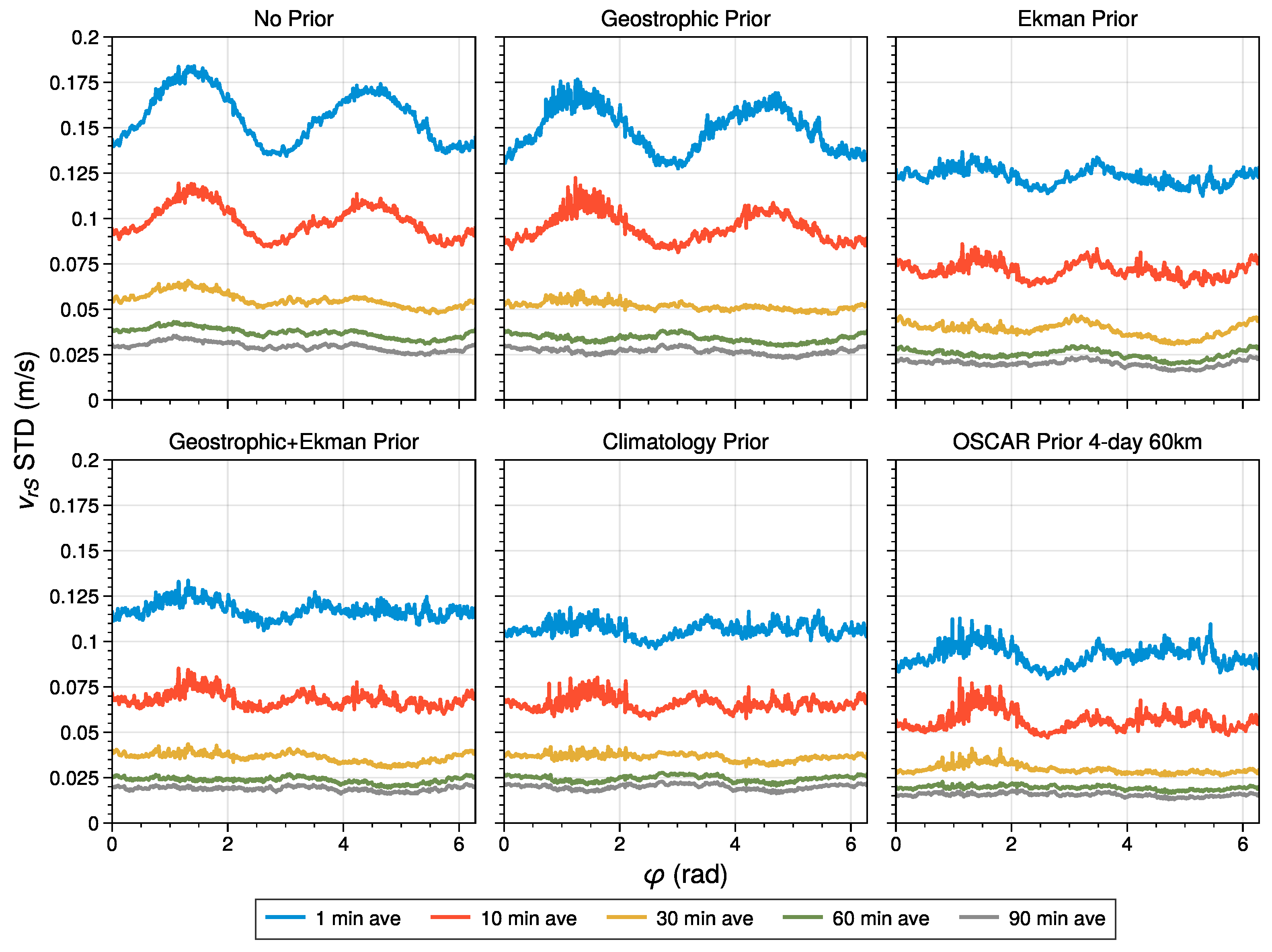
This azimuth dependence can be seen in Figure 11 or different ocean prior corrections. When no correction is applied, there is a significant modulation of the signal with . The modulation disappears with increased averaging time, as the error is reduced but spread out from the location of the strong currents, as illustrated in Figure 10, panels c. and d. The inclusion of the geostrophic (AVISO-like) does little to reduce the modulation, since both the Equatorial and Southern Ocean currents have significant wind-driven contributions. The magnitude of the modulations is reduced significantly if one includes priors which have wind-driven currents, as can be expected from the global distribution of residual radial velocity errors shown in Figure 4.
The calibration method examined here examines the viability of meeting a global requirement for ocean surface leakage using only one averaging time for the entire globe. This is certainly not optimal, as the averaging time could be varied to minimize leakage away from areas which contaminate the estimates significantly and the estimates from these regions can be down-weighted when computing the optimal estimate for the pointing. As this more optimal algorithm will be geographically dependent, as well as dependent on the performance of the ocean prior, we leave a detailed optimal algorithm for future work, and concentrate here on showing that the simpler algorithm is sufficient to meet the ODYSEA mission requirements.
Similar considerations will likely apply to regions, such as the Mediterranean Sea or near-coastal zones, where land contamination effects will limit the data that can be included in the averaging.
4. Discussion and Conclusions
While Doppler scatterometers for ocean surface current mapping have been demonstrated successfully from airborne platforms, scaling the measurement to a spaceborne instrument becomes more challenging, as the knowledge of the pointing of the radar antenna must be better by almost two orders of magnitude. Furthermore, the airborne techniques used to estimate this pointing error no longer apply, since they cannot be implemented with the satellite orbit geometry. Given the potential NASA/CNES ODYSEA mission, this issue becomes critical to address when assessing its feasibility.
In this paper, we have demonstrated a proof-of-concept approach for calibrating the pointing error, given that it behaves in a feasible way with a systematic dependence on the azimuth angle and a temporal variability characterized by a given correlation time. While specific mechanical implementations of the instrument may be able to improve this model by using detailed parametric models, our goal is to demonstrate that a simple generic model with limited parameters can be used to meet the ODYSEA error budget needs.
The major challenges to be overcome by the along-track averaging technique used here were the contamination of the estimate by ocean current leakage and the limitations imposed by the temporal variability of the error. We found that reducing ocean leakage required along-track averaging of at least 10 minutes, if no ocean corrections were applied. We then examined improvements based on various models of ocean currents that might be available now or in the next decade. We found that using these ocean priors, we could reduce the required averaging time from one-half to one-quarter, depending on the skill of the mode.
The angular characteristics of the error were shown to be a major factor in determining the amount of ocean leakage that would be present. We found that constant pointing biases or low-order harmonics dominated the ocean leakage contamination. These errors introduce basin-scale distortions which may be negligible when examining the ocean mesoscales (i.e., scales smaller than ∼300 km), but may be limiting for basin-scale absolute currents (e.g., net Equatorial wind-work). On the other hand, given current capabilities to constrain spacecraft distortions, the temporal variability of the pointing errors played a significantly smaller role. An even smaller role was played by the random measurement errors.
Finally, we showed that, although using a single along-track averaging time was sufficient to meet calibration requirements globally, geographically localized leakage could result in larger errors or larger temporal stability requirements. We pointed out that a future implementation of this algorithm should tune the averaging times depending on geographical ocean signals, a task for future work.
For the moment, we conclude that using a simple, reduced parameter, calibration process is sufficient for meeting ODYSEA measurement requirements. Future developments will only improve this assessment. The algorithm is general enough that it can be translated easily for other potential Doppler scatterometer missions, such as the OSCOM mission proposed by [22].
Author Contributions
ER conceived the calibration algorithm, did the analysis for simulation results and wrote the paper; HT sampled the model data and generated the simulated AVISO and OSCAR-like prior datasets; AW built the measurement simulator and was the link to the ODYSEA design; CU and AB independently validated the ocean leakage results, advised on simulating the geostrophic priors, and suggested an optimal time averaging strategy.
Funding
This work was performed at the Jet Propulsion Laboratory, California Institute of Technology under prime contract with NASA (80NM0018D0004), and was awarded under NASA Research Announcement (NRA) NNH17ZDA001N-EVS3, Research Opportunities in Space and Earth Science (ROSES-2017), Appendix A.34: Earth Venture Suborbital-3; NASA Sub-Mesoscale Ocean Dynamics Experiment (NASA S-MODE). Datlas work was funded by the "Centre National d’Etudes Spatiales" grant DTN/TPI/TR-2024.0015117.
Data Availability Statement
LLC-4320 model output is accessible through the National Aeronautics and Space Administration research center (https://data.nas.nasa.gov/ecco).
Acknowledgments
This work was performed at the Jet Propulsion Laboratory, California Institute of Technology under prime contract with NASA (80NM0018D0004). High-End Computing was provided by the NASA Advanced Supercomputing (NAS) Division at the Ames Research Center. Copyright 2024 California Institute of Technology. US government sponsorship acknowledged
Conflicts of Interest
The authors declare no conflicts of interest.
References
- Rodríguez, E.; Wineteer, A.; Perkovic-Martin, D.; Gál, T.; Stiles, B.W.; Niamsuwan, N.; Rodriguez Monje, R. Estimating ocean vector winds and currents using a Ka-band pencil-beam Doppler scatterometer. Remote Sensing 2018, 10, 576. Publisher: MDPI. [CrossRef]
- Goldstein, R.M.; Zebker, H.A. Interferometric radar measurement of ocean surface currents. Nature 1987, 328, 707–709. Publisher: Nature Publishing Group. [CrossRef]
- Rodríguez, E.; Bourassa, M.; Chelton, D.; Farrar, J.T.; Long, D.; Perkovic-Martin, D.; Samelson, R. The winds and currents mission concept. Frontiers in Marine Science 2019, 6, 438. Publisher: Frontiers Media SA. [CrossRef]
- Rodriguez, E. On the optimal design of doppler scatterometers. Remote Sensing 2018, 10, 1765. Publisher: MDPI. [CrossRef]
- Wineteer, A.; Torres, H.S.; Rodriguez, E. On the Surface Current Measurement Capabilities of Spaceborne Doppler Scatterometry. Geophysical Research Letters 2020, 47, e2020GL090116. [CrossRef]
- Torres, H.; Wineteer, A.; Klein, P.; Lee, T.; Wang, J.; Rodriguez, E.; Menemenlis, D.; Zhang, H. Anticipated Capabilities of the ODYSEA Wind and Current Mission Concept to Estimate Wind Work at the Air–Sea Interface. Remote Sensing 2023, 15, 3337. Number: 13 Publisher: Multidisciplinary Digital Publishing Institute. [CrossRef]
- Lee, T.; Gille, S.; Ardhuin, F.; Bourassa, M.; Chang, P.; Cravatte, S.; Dibarboure, G.; Farrar, T.; Fewings, M.; Girard-Ardhuin, F. ODYSEA: a satellite mission to advance knowledge of ocean dynamics and air-sea interaction 2025.
- Farrar, J.T.; D’Asaro, E.; Rodriguez, E.; Shcherbina, A.; Lenain, L.; Omand, M.; Wineteer, A.; Bhuyan, P.; Bingham, F.; Villas Boas, A.B. S-mode: The sub-mesoscale ocean dynamics experiment. Bulletin of the American Meteorological Society 2025. Publisher: American Meteorological Society.
- Torres, H.S.; Rodriguez, E.; Wineteer, A.; Klein, P.; Thompson, A.F.; Callies, J.; D’Asaro, E.; Perkovic-Martin, D.; Farrar, J.T.; Polverari, F. Airborne observations of fast-evolving ocean submesoscale turbulence. Communications Earth & Environment 2024, 5, 771. Publisher: Nature Publishing Group UK London.
- Wineteer, A.; Rodriguez, E.; Martin, D.P.; Torres, H.; Polverari, F.; Akbar, R.; Rocha, C. Exploring the Characteristics of Ocean Surface Winds at High Resolution With Doppler Scatterometry. Geophysical Research Letters 2024, 51, e2024GL113455. [CrossRef]
- Rodriguez, E.; Fernandez, D.E.; Peral, E.; Chen, C.W.; De Bleser, J.W.; Williams, B. Wide-swath altimetry: a review. Satellite altimetry over oceans and land surfaces 2017, pp. 71–112. Publisher: CRC Press.
- Dibarboure, G.; Ubelmann, C.; Flamant, B.; Briol, F.; Peral, E.; Bracher, G.; Vergara, O.; Faugère, Y.; Soulat, F.; Picot, N. Data-Driven Calibration Algorithm and Pre-Launch Performance Simulations for the SWOT Mission. Remote Sensing 2022, 14, 6070. Number: 23 Publisher: Multidisciplinary Digital Publishing Institute. [CrossRef]
- Ubelmann, C.; Dibarboure, G.; Flamant, B.; Delepoulle, A.; Vayre, M.; Faugère, Y.; Prandi, P.; Raynal, M.; Briol, F.; Bracher, G.; et al. Data-Driven Calibration of SWOT’s Systematic Errors: First In-Flight Assessment. Remote Sensing 2024, 16, 3558. Number: 19 Publisher: Multidisciplinary Digital Publishing Institute. [CrossRef]
- Torres, H.S.; Klein, P.; Menemenlis, D.; Qiu, B.; Su, Z.; Wang, J.; Chen, S.; Fu, L.L. Partitioning Ocean Motions Into Balanced Motions and Internal Gravity Waves: A Modeling Study in Anticipation of Future Space Missions. Journal of Geophysical Research: Oceans 2018, 123, 8084–8105. _eprint: https://onlinelibrary.wiley.com/doi/pdf/10.1029/2018JC014438. [CrossRef]
- Molod, A.; Takacs, L.; Suarez, M.; Bacmeister, J. Development of the GEOS-5 atmospheric general circulation model: evolution from MERRA to MERRA2. Geoscientific Model Development 2015, 8, 1339–1356. Publisher: Copernicus GmbH. [CrossRef]
- Strobach, E.; Molod, A.; Trayanov, A.; Forget, G.; Campin, J.M.; Hill, C.; Menemenlis, D. Three-to-Six-Day Air–Sea Oscillation in Models and Observations. Geophysical Research Letters 2020, 47, e2019GL085837. _eprint: https://onlinelibrary.wiley.com/doi/pdf/10.1029/2019GL085837. [CrossRef]
- Arbic, B.; Alford, M.; Ansong, J.; Buijsman, M.; Ciotti, R.; Farrar, J.T.; Hallberg, R.; Henze, C.; Hill, C.; Luecke, C.; et al. A Primer on Global Internal Tide and Internal Gravity Wave Continuum Modeling in HYCOM and MITgcm. New Frontiers In Operational Oceanography 2018, pp. 307–391.
- Pujol, M.I.; Faugère, Y.; Taburet, G.; Dupuy, S.; Pelloquin, C.; Ablain, M.; Picot, N. DUACS DT2014: the new multi-mission altimeter data set reprocessed over 20 years. Ocean Science 2016, 12, 1067–1090. Publisher: Copernicus GmbH. [CrossRef]
- Bonjean, F.; Lagerloef, G.S.E. Diagnostic Model and Analysis of the Surface Currents in the Tropical Pacific Ocean. Journal of Physical Oceanography 2002, 32, 2938–2954. Publisher: American Meteorological Society Section: Journal of Physical Oceanography. [CrossRef]
- Chelton, D.B.; Schlax, M.G.; Samelson, R.M.; Farrar, J.T.; Molemaker, M.J.; McWilliams, J.C.; Gula, J. Prospects for future satellite estimation of small-scale variability of ocean surface velocity and vorticity. Progress in Oceanography 2019, 173, 256–350. Publisher: Elsevier. [CrossRef]
- of Sciences, N.A.; Medicine.; on Engineering, D.; Sciences, P.; Board, S.S.; on the Decadal Survey for Earth Science, C.; from Space, A. Thriving on our changing planet: A decadal strategy for Earth observation from space; National Academies Press, 2019.
- Du, Y.; Dong, X.; Jiang, X.; Zhang, Y.; Zhu, D.; Sun, Q.; Wang, Z.; Niu, X.; Chen, W.; Zhu, C. Ocean surface current multiscale observation mission (OSCOM): Simultaneous measurement of ocean surface current, vector wind, and temperature. Progress in Oceanography 2021, 193, 102531. Publisher: Elsevier. [CrossRef]
Figure 1.
Cross-track spatial signature of velocity errors (normalized for clarity) induced by different harmonics in the Fourier expansion of as a function of distance from the nadir. The solid orange/blue lines are the errors in the along/across-track velocities. The dashed lines represent the residual errors after removing wavelengths greater than 130 km.
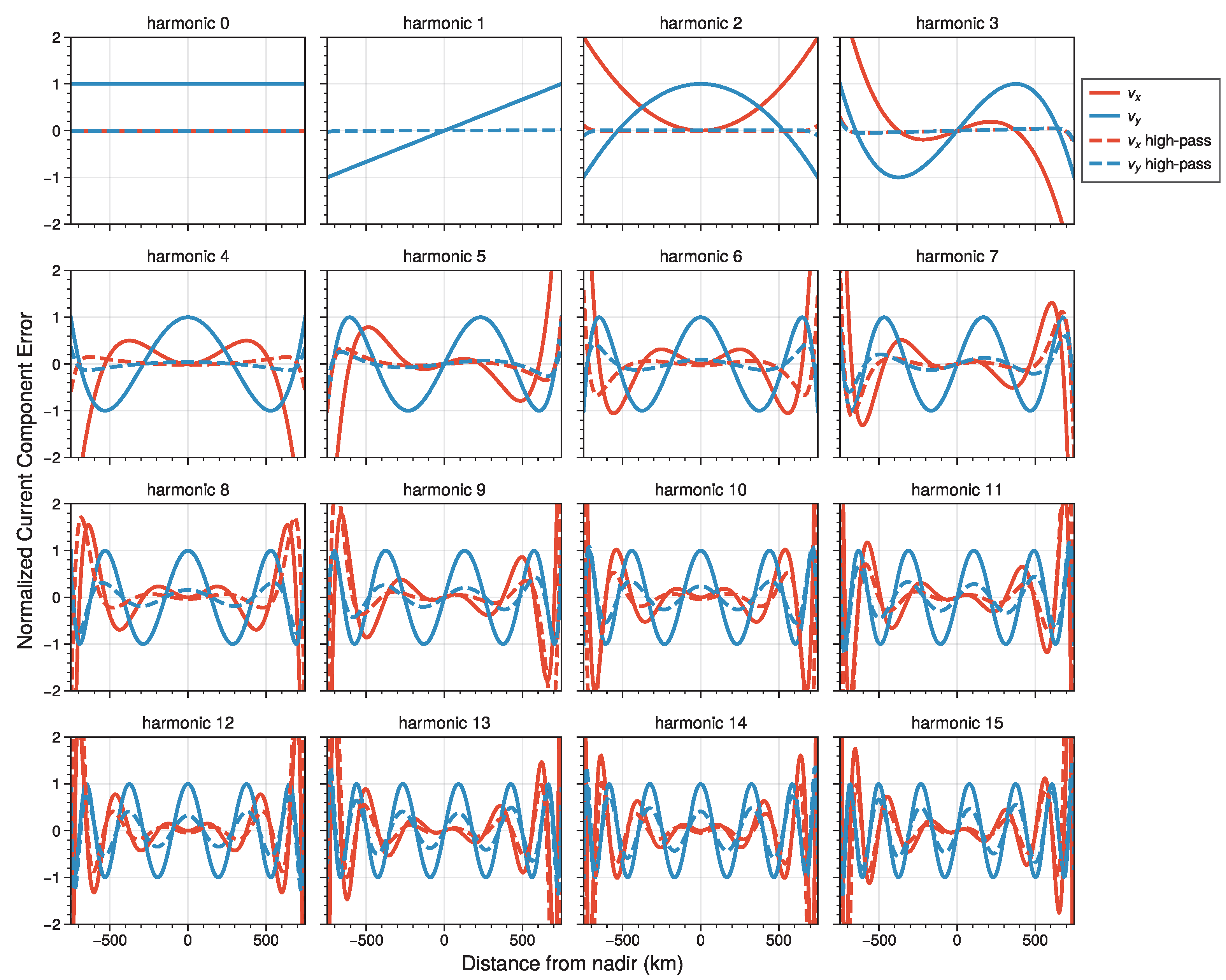
Figure 2.
Space-time spectra for ocean simulation and satellite-like priors. a) spectrum of the Coupled Ocean Atmosphere Simulation (COAS); b) spectrum of the PO.DAAC OSCAR product; b) spectrum for the OSCAR-like product; c) spectrum for the AVISO-like (geostrophic) product. The spectrum were computed in the Kuroshio Extension region. The gray rectangle in panel a) highlights the spectral coverage of ODYSEA sampling.
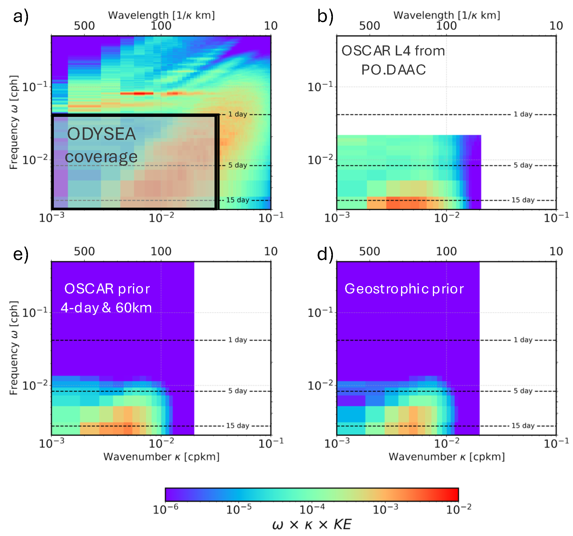
Figure 3.
Wind-driven current model parameters as a function of latitude. The estimates for the bias and slope parameters for each latitude band is plotted as a point, and a spline fit through the data, which will be used to smooth and interpolate the results, is plotted as solid line. The top row shows the results for the magnitude of the wind driven current, while the bottom row shows the angle of the current relative to the wind. The left column shows the constant value, while the right column shows the constant of proportionality with the wind speed, .
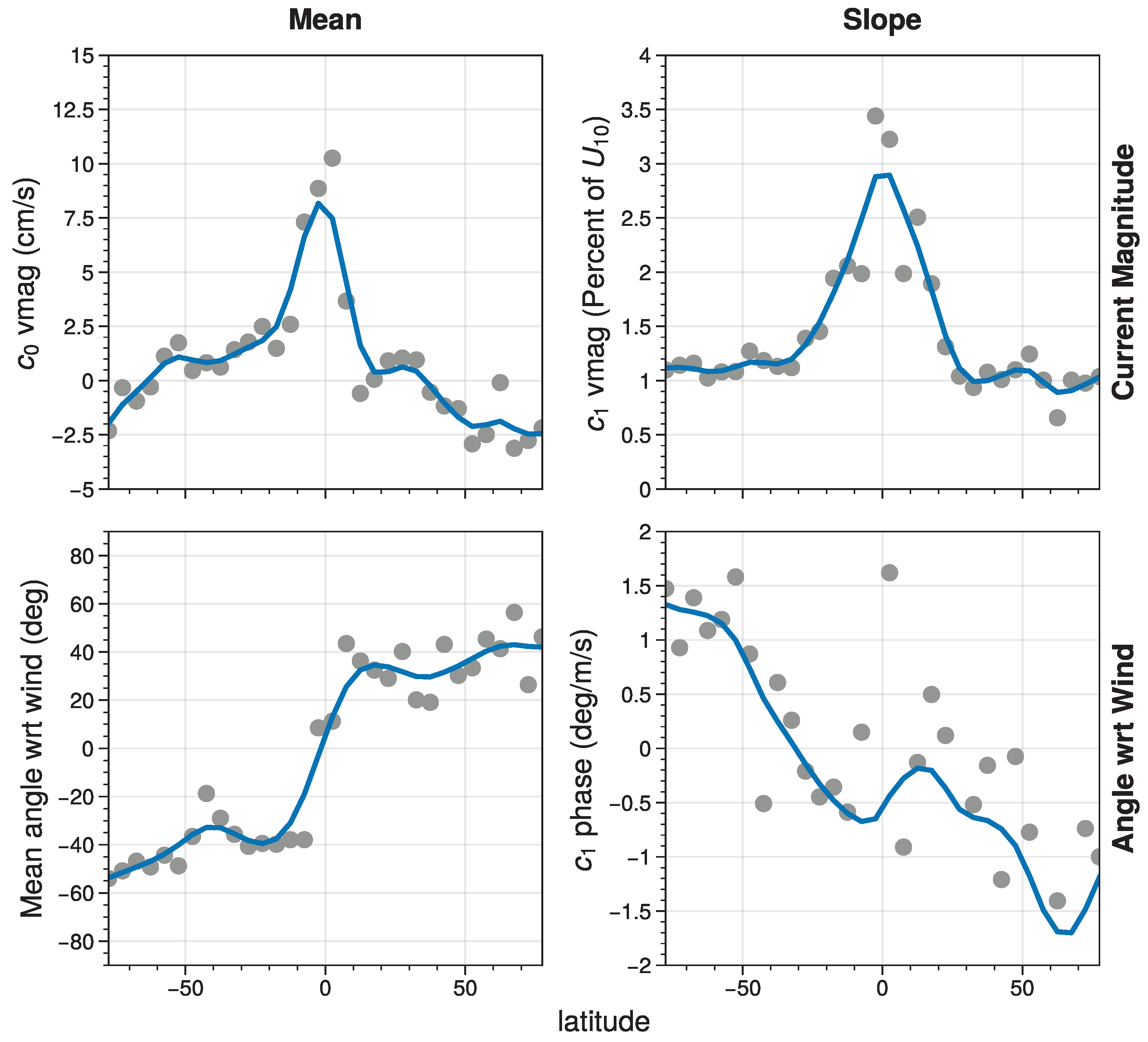
Figure 4.
Residual radial velocity after subtracting prior models for two-weeks of data. The left-hand column shows the mean difference, while the right-hand column shows the standard deviation of the differences. The top row shows the ocean leakage without removing any priors, and subsequent rows show the residuals after subtracting: 2) geostrophic (AVISO-like) model, 3) the wind-driven (Ekman-like) current model; 4) the sum of geostrophic and wind-driven models; 5) climatology; and, 6) the OSCAR-like model.

Figure 5.
(left) Radial velocity leakage as a function of averaging time with and without ocean priors as a function of along-track averaging time. The error allocation for ODYSEA is shown as a dashed line. (center, right) Derived pointing errors for the along-track (center) and cross-track (right) surface velocity components. The solid/dashed lines are the errors evaluated of the performance/vector swaths, while the black dashed lines represent the derived surface component measurement requirements for each swath.
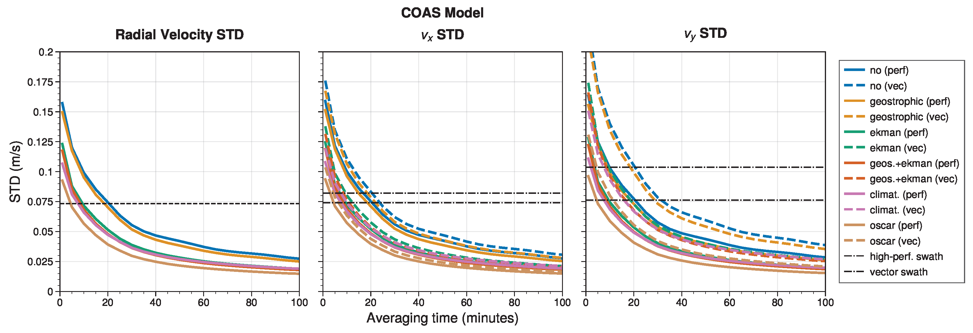
Figure 6.
(solid lines) Spectra of ocean leakage for no prior (left), geostrophic+Ekman (middle), and OSCAR-like priors, for a variety of averaging times. Also shown (dashed lines) are the spectra for the 50 cm/s at 5 km random errors after similar temporal averaging. For reference, a black dashed line showing an spectrum is included.
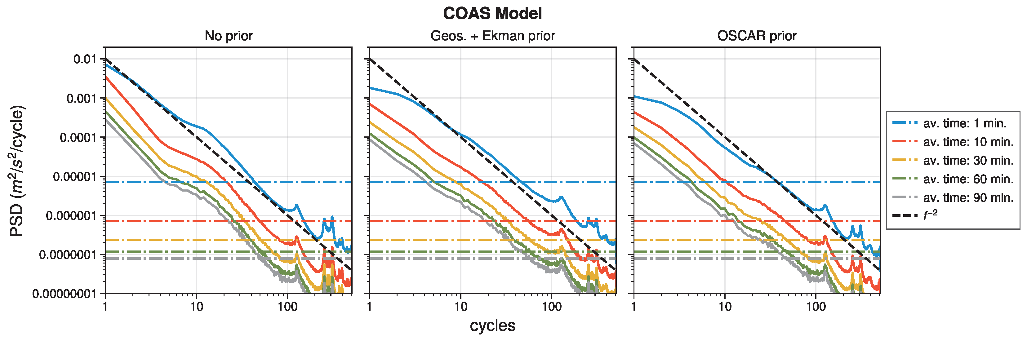
Figure 7.
Ocean leakage after removing a progressively larger number of low-frequency harmonics for the various prior models examined.
Figure 7.
Ocean leakage after removing a progressively larger number of low-frequency harmonics for the various prior models examined.
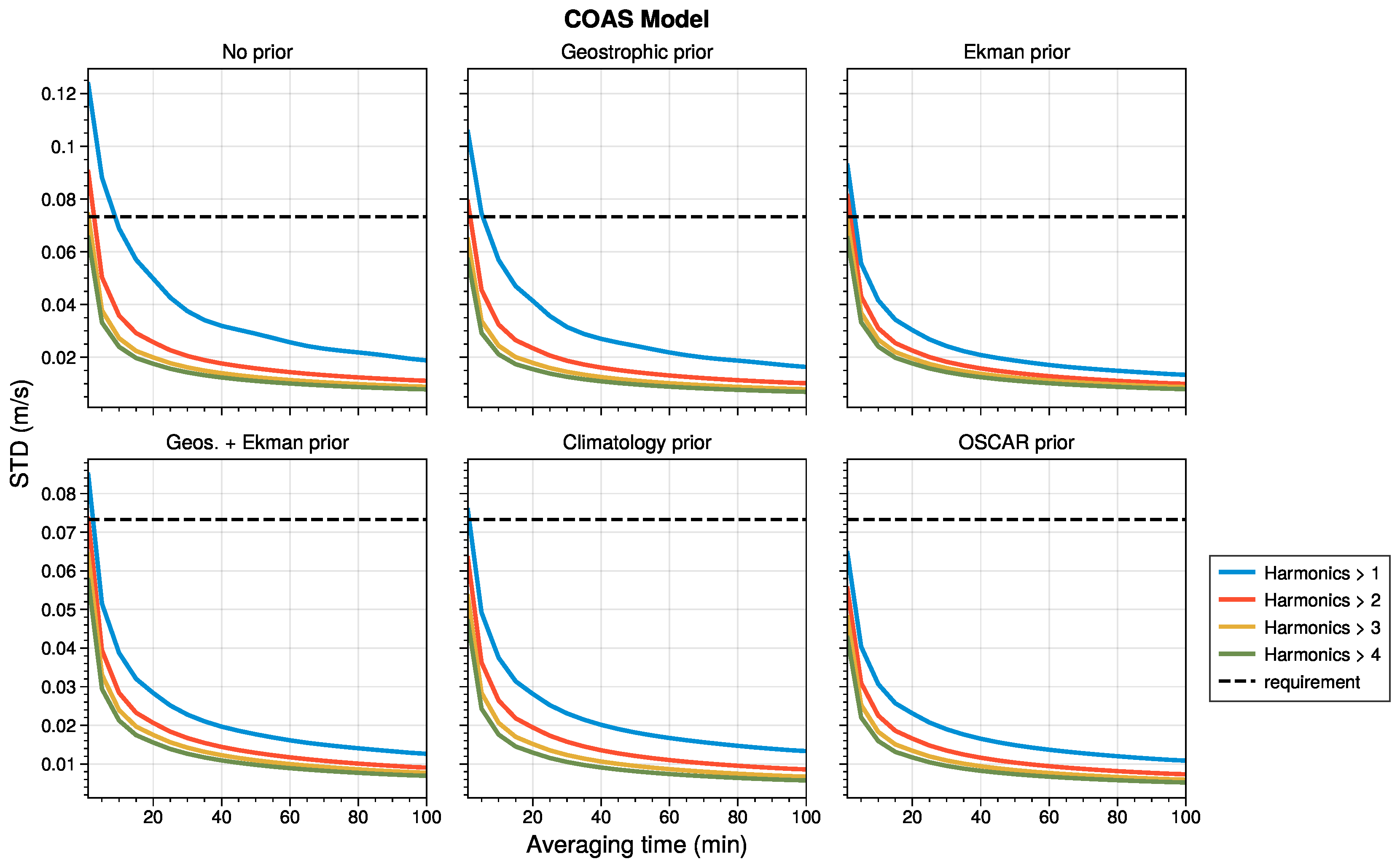
Figure 8.
Radial velocity leakage as a function of averaging time and increasing number of orbit averaging. Without prior (left). With a mean current prior (right). The error allocation for ODYSEA is shown as a horizontal black dashed line.
Figure 8.
Radial velocity leakage as a function of averaging time and increasing number of orbit averaging. Without prior (left). With a mean current prior (right). The error allocation for ODYSEA is shown as a horizontal black dashed line.
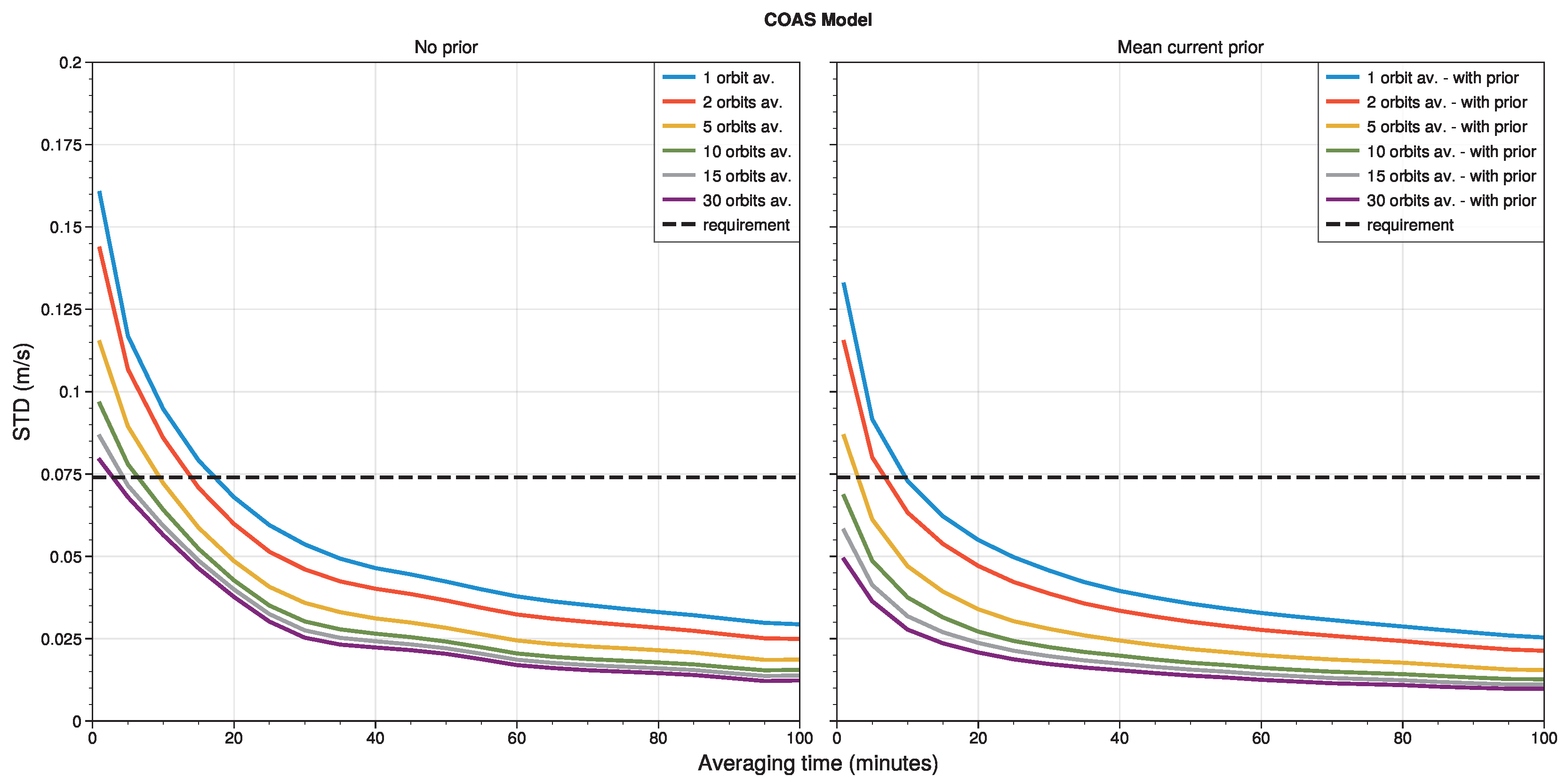
Figure 9.
Swath-averaged radial velocity error as a function of pointing error correlation time. In the top row, the error is dominated by , while on the bottom row, the spin harmonic coefficients dominate. The harmonic error is assigned a power-law behavior: (first column), (second column), and (third column). The different lines, coded by color, show different along-track averaging times. The dashed black line shows the required radial velocity error.
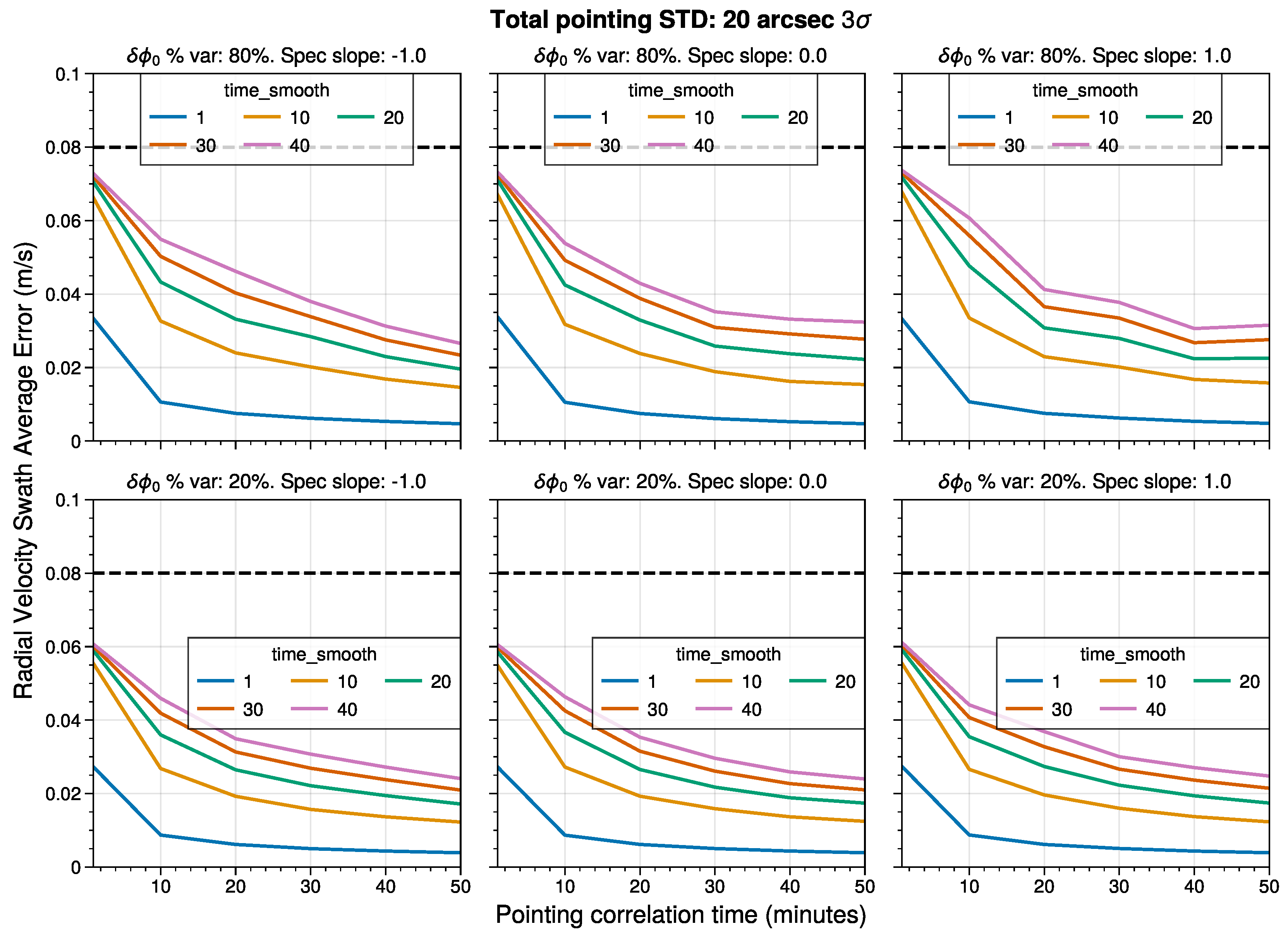
Figure 10.
a. Instantaneous radial velocity signal for three orbit cycles of the ODYSEA instrument. b. The same as a., but after applying a constant pointing error with 50 cm/s pointing error. c. Residual radial velocity errors after applying the 10-minute along-track average pointing calibration. d. Same as c., but after applying a 40-minute along-track average pointing correction.
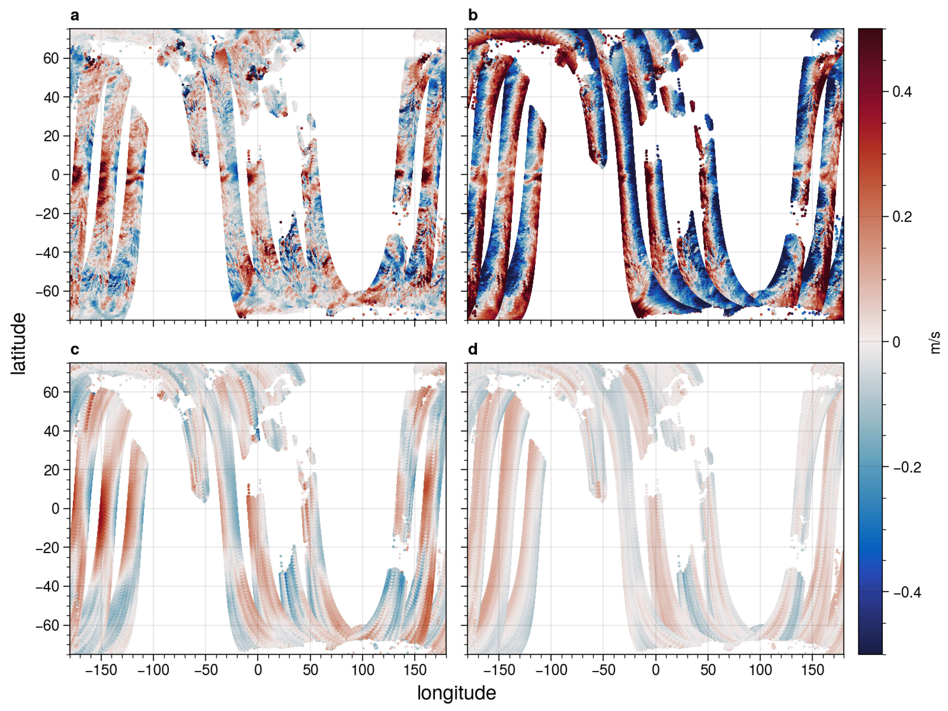
Figure 11.
Radial velocity leakage standard deviation as a function of , the azimuth angle relative to the platform heading. The various panels illustrate the impact of applying various models for ocean priors. Different along-track averaging times are indicated by varying line color.
Figure 11.
Radial velocity leakage standard deviation as a function of , the azimuth angle relative to the platform heading. The various panels illustrate the impact of applying various models for ocean priors. Different along-track averaging times are indicated by varying line color.
Disclaimer/Publisher’s Note: The statements, opinions and data contained in all publications are solely those of the individual author(s) and contributor(s) and not of MDPI and/or the editor(s). MDPI and/or the editor(s) disclaim responsibility for any injury to people or property resulting from any ideas, methods, instructions or products referred to in the content. |
© 2025 by the authors. Licensee MDPI, Basel, Switzerland. This article is an open access article distributed under the terms and conditions of the Creative Commons Attribution (CC BY) license (http://creativecommons.org/licenses/by/4.0/).
Copyright: This open access article is published under a Creative Commons CC BY 4.0 license, which permit the free download, distribution, and reuse, provided that the author and preprint are cited in any reuse.


