Submitted:
09 July 2025
Posted:
09 July 2025
You are already at the latest version
Abstract
Currently, the shear strength of coarse-grained soil is commonly determined using the Duncan formula, which establishes a relationship between the shear strength and confining pressure. Specifically, the parameters of the Duncan formula are estimated based on available test data using least squares regression, which mitigates the limitations associated with small sample sizes and significant errors in the classic grouping method. However, hypothesis testing in mathematical statistics reveals that the residual variances from the classic least squares estimation exhibit heteroscedasticity and autocorrelation, violating the fundamental assumptions required for least squares regression. Consequently, parameter estimates obtained through classic least squares regression have large variances, leading to unreliable statistical inferences. To address this issue, we propose a generalized least squares method that corrects for heteroscedasticity and autocorrelation of the residuals. Triaxial test data for five different coarse-grained soil materials are analyzed using the proposed method. The results show that the mean values of the estimated parameters of the Duncan formula are close to those obtained using the classic method, while their variances are significantly reduced, demonstrating the effectiveness of the proposed approach.
Keywords:
coarse-grained soil
; shear strength
; variance
1. Introduction
Coarse-grained soil has the advantages of easy accessibility, low cost, and high permeability and is therefore widely utilized in engineering projects such as roads, earth-rock dams, land reclamation, and high-fill airports. The shear strength of coarse-grained soil is a critical technical parameter as it directly affects both project safety and investment benefits.
The guidelines for determining the standard soil shear strength vary among different standards. For instance, the Design Code for Rolled Earth-Rock Fill Dams (SL274-2020) and standard NB/T10872-2021. stipulate that the standard value should be the average of the minimum shear strength. These specifications also define the required number of test groups: for anti-seepage soil materials, at least 11 groups are required, and each group contains 4–6 confining pressure levels. For coarse-grained materials, NB/T10872-2021 mandates a minimum of six test groups, whereas SL274-2020 requires at least 11 groups for both fine-grained soil and coarse-grained soil. The Unified Standard for Reliability Design of Hydraulic Engineering Structures (GB5099-2013) recommends using the 0.1 quantile of the probability distribution as the standard value for the strength of geotechnical materials and artificial foundations. In addition, the Code for Investigation of Geotechnical Engineering (GB 50021-2001, 2009 Edition) specifies that the standard value of a geotechnical parameter should be based on the one-sided confidence limit of the confidence interval for the mean value of the parameter matrix, which is derived using statistical interval estimation theory. By simplifying this approach, the relationship between the standard value and the mean value can be expressed as follows:
where is the coefficient of variation, which is the ratio of the standard deviation to the mean. n is the number of groups.
Apparently, it is equally important to determine the mean and variance (or standard deviation) of the soil shear strength for engineering practices.
Currently, the shear strength of coarse-grained soil is predominantly represented by the Duncan formula. In reliability analyses of the anti-sliding stability and foundation bearing capacity of coarse-grained soil, it is essential to predefine the variance of the parameters. Therefore, it is crucial to investigate the variance of the variables in the Duncan formula for determining the nonlinear shear strength of coarse-grained soil (Aghchai et al., 2020).
2. Nonlinear Shear Strength of Coarse-Grained Soil
The shear strength of soil is generally described by the Mohr-Coulomb theory:
where is the shear strength of the soil, is the normal stress on the shear plane, and are the cohesion (or interlocking force) and internal friction angle of the soil, and are the major and minor principal stresses at the limit equilibrium failure point in the triaxial test.
Typically, the indices c and are constants. However, for coarse-grained soil, the shear strength exhibits strong nonlinearity; hence, it is necessary to define these indices within a limited confining pressure range. In contrast to the linear relationship observed under low confining pressure conditions, under high confining pressure conditions, the strength envelope deviates from a straight line. To characterize the shear strength of coarse-grained soil across a wide confining pressure range, the following approaches have been employed in engineering practices. The first method involves a segmented description, in which different values of c and are used for low (typically 100–800 kPa) and high confining pressure conditions. Another approach directly models the curved envelope of the shear strength, such as the Demeler formula and the Duncan formula
where and are the shear strength coefficient and exponent. is the internal friction angle when the confining pressure is equal to the standard atmosphere, and is the decrease in the friction angle when the confining pressure increases by 10 times. According to the Duncan formula, the friction angle is expressed as follows: .
There are two methods for determining nonlinear strength indices. In the first method, the strength indices and are determined based on the test groups, and then, their minimum average values are determined. In the second method, the minimum average values of and under each confining pressure are determined first, and then, the friction angle is calculated based on these minimum average values. Finally, the strength indices are determined based on the Duncan formula. The parameters derived using these two methods differ and both methods suffer from an insufficient number of grouped samples, leading to large errors and a low accuracy for intermediate transition variables. To address this issue, all test data should be utilized, and the least squares method should be used to directly estimate the nonlinear strength parameters (Chen et al., 2019; Cao et al., 2007).
Linear regression for estimating Duncan’s nonlinear shear strength parameters of coarse-grained soil.
where is the independent variable, which is a non-random variable. is the dependent variable, which is a random variable. and − are the parameters to be determined.
The prerequisite of this method is that the regression residuals meet the requirements of classic least squares estimation.
3. Classic Least Squares Estimation
The linear regression model is as follows:
where is the residual term or the error term, which represents the influences of factors other than on the friction angle and the measurement error.
If the residual term satisfies the following three conditions, then the least squares regression is valid: (a) the mathematical expectation is , (b) the residuals under different confining pressures have equal variances, that is, , (), and (c) the residuals under different confining pressures are uncorrelated, that is, , . The above is the Gauss-Markov hypothesis.
The least squares method finds estimates of and − that minimize the square of the length of the residual vector , i.e.,.
By expanding this formula and taking partial derivatives with respect to and − and setting them equal to zero, and − can be obtained.
By substituting n sets of observation data into the above equation, we can obtain estimated values of and −.
4. Homogeneity of Variance and Correlation Test of the Residuals of the Duncan Formula Estimated VIA Least Squares Regression
Currently, the prerequisite of the least squares method is generally not tested when determining the shear strength parameters of soil. Chen et al. (2005) noticed the variance of the regression residuals and proposed that the weighted least squares method be applied to improve the regression. The weighting coefficient is , and are obtained via linear regression of the residuals and independent variables. This approach partially eliminates the variance of the residuals, but it does not fundamentally solve the problem. In the regression method recommended by the specification, i.e., , the independent variable is also a random variable. Based on this characteristic, Yu et al. (2012) proposed that the orthogonal least squares method be applied to correct the shear strength estimated based on regression using -. The above methods only involve regressions of the parameters of the Mohr-Coulomb formula, which only partially eliminates the variance of the regression residuals. To the best of our knowledge, the variance and correlation of the residuals in nonlinear regression of the shear strength of coarse-grained soil has not been studied (Chen et al., 2007; Gong et al., 2020; Gong et al., 2018).
4.1. Regression Residuals and the Covariance Matrix
Based on the test results for several coarse-grained materials from the sites of engineering projects, the nonlinear shear strength was determined to examine the variance and correlation of the residuals in the nonlinear strength regression. Specifically, in the triaxial test on coarse-grained granite from Area I of earth-rock dam project A, twelve sets of parallel tests were conducted under six confining pressure conditions (i.e., 100, 500, 1000, 1500, 2000, and 2500 kPa). The regression equation is shown in Figure 1, and the regression residuals are shown in Figure 2. As can be seen from Figure 2, the distribution of the residuals varies across the different confining pressures, indicating that the variance of the residuals is not uniform. To determine whether the residuals under the six confining pressures are correlated, it is necessary to test the covariance matrix of the residuals. The regression residuals of the friction angle from the triaxial tests were calculated, and the residual covariance matrix was obtained:
It can be seen that the main diagonal elements of the residual covariance matrix are not equal, and the non-diagonal elements are not zero, suggesting variance homogeneity and correlation of the residuals. In order to accurately determine the homogeneity and correlation of the regression residuals, hypothesis testing is required.
First, the Kolmogorov–Smirnov (K-S) method was applied to test whether the residuals as a whole satisfy the assumption of a normal distribution. Next, assuming that the ratio of the sample variances of the regression residuals at each confining pressure level follows the F-distribution, the sample variance at each confining pressure was calculated to test whether the residual variances were consistent across different confining pressures under a certain probability level (quantile). This step corresponds to the variance homogeneity test. Finally, the correlation of the regression residuals under different confining pressure levels was examined.
4.2. K-S Test for Normal Distribution of Regression Residuals
(1) Null hypothesis : and alternative hypothesis : , where is the given normal distribution function. (2) The test statistic is selected as the principal variable. When the null hypothesis is true, the test statistic is . At the significance level , if , then the null hypothesis is rejected, where is an appropriate constant. Kolmogorov derived the limiting distribution of and tabulated it. (3) The rejection region is determined. For a given significance level that satisfies , the quantile is the critical value, and the rejection region is .
Table 1 presents the regression residuals for the coarse-grained granite from Area I of project A under various confining pressure conditions. The mean and standard deviation of all of the residuals are 2.6659 10−4 and 1.6573. For a significance level of 0.01, 0.01, and t 1.63, which is taken as an approximate value of . Then, the rejection region is ).
0.1782. Because
0.1782 = 1.5119, and it falls outside the rejection region [1.63, +), we accept the hypothesis that the regression residuals of the shear strength are normally distributed.
4.3. Homogeneity Test of Regression Residuals Under Different Confining Pressure Conditions
Theoretical studies have shown that the F-test is sensitive to deviations from homogeneity of variance, making it suitable for testing the variance of residuals under different confining pressures. The null hypothesis H0 and alternative hypothesis H1 are
and , , , , and they are not all equal.
Determine the rejection region.
Let ,
and .
Then, the rejection region is (0, 0.2874] and [3.48, +.
Table 2 shows the sample variance ratios of the regression residuals under various confining pressures and whether they are in the rejection region. indicates that the variance ratio is in the acceptance region and the null hypothesis is accepted, while indicates that the variance ratio is in the rejection region and the null hypothesis is not accepted.
It can be seen that except for the diagonal elements where the variance ratio is equal to 1, seven of the sample variance ratios of the residuals under different confining pressures are in the acceptance region and eight are in the rejection region. Therefore, the variance homogeneity hypothesis is not accepted.
4.4. Residual Independence Test Under Different Confining Pressure Conditions
Assuming that the regression residuals under different confining pressures are two different random variables U and V, the independence test is equivalent to testing their correlation coefficient . The null hypothesis H0 and alternative hypothesis H1 are
0. The sample correlation coefficient R is used as the point estimator of
. R is shown in Table 3.
When is true,
It follows a t-distribution with degrees of freedom of . t can be found in Table 4. Given a significance level ,
If the observed value of t satisfies , then the null hypothesis is rejected.
, and =1.812.
The rejection regions are (0, −1.812] and [1.812, +.
It can be seen that seven of the above t values are within the rejection region. Therefore, the independence hypothesis of the residuals under each confining pressure is rejected.
The regression residual analysis of the nonlinear shear strength based on the Duncan formula for the coarse-grained soils from three engineering projects (projects A, B, and C) indicates that the diagonal elements of the covariance matrix of the least squares regression residuals for the nonlinear shear strength friction angle are not equal, and the non-diagonal elements are not zero. Although the probability distribution of the residuals passes the normality test, the residuals under different confining pressures exhibit homogeneity of variance and irrelevance. This confirms the occurrence of residual variance heteroscedasticity and autocorrelation across the different confining pressures.
5. Elimination of Residual Variance Heteroscedasticity and Autocorrelation
If the residuals exhibit heteroscedasticity and autocorrelation, the regression equation no longer meets the prerequisites of least squares regression. In this case, if the least squares method is used, although the estimated values of the parameters are unbiased, the variances of the parameters could deviate from the actual value. A solution is to replace the regression variables. For the linear regression equation
where , ‘. , and are the confining pressure and friction angle of the th test. The symbol ‘ denotes matrix transposition. is the covariance matrix of the residual vector under different confining pressures. is the variance of the residual vector.
It can be seen that the covariance matrix of the residual is not an identity matrix. is nonsingular and positive definite, and there exists a nonsingular symmetric matrix such that , that is, the matrix is the square root matrix of .
By defining new variables (Wang et al., 2021; Douglas et al., 2022), namely,
the regression equation becomes , i.e.,
After this transformation, the model residuals have a zero mean, i.e., =0, and the covariance matrix of is
Therefore, has a zero mean, constant variance, and uncorrelated variance. Equation (14) satisfies the general assumptions of the classic least squares estimation, and the least squares function is
The canonical equation for least squares is
The solution to the equation is
6. Examples
The triaxial test data for five types of coarse-grained materials used in three engineering projects (A, B, and C) were used to perform classic least squares regression and regression after eliminating the heteroscedasticity and autocorrelation of the residual variance. After obtaining the regression equation, the covariance matrix of the parameters was calculated (Table 5).
It can be seen that for each coarse-grained material, the regression parameters obtained using the two methods are similar, yet the variances of the parameters are reduced when the proposed method is applied.
For example, for the coarse-grained material from Area II of Project A, the regression equation from the classic least squares method and the covariance matrix between are
After eliminating the residual variance heteroscedasticity and autocorrelation, the regression equation and covariance matrix are
It can be seen that after eliminating the heteroscedasticity and autocorrelation, the parameter variance is reduced, providing more accurate estimates of the shear strength parameters of the coarse-grained soil.
7. Conclusions
The shear strength of coarse-grained soil has strong non-linearity and is commonly determined using the Duncan formula. However, the classic grouping method for estimating the parameters has the limitations of small sample sizes and large errors. When the classic least squares method is applied to estimate the Duncan shear strength parameters based on triaxial test data, it has been found that the residual variance exhibited heteroscedasticity and autocorrelation, which violates the prerequisites of the least squares method. In this study, we introduced a generalized least squares method to eliminate these issues. By analyzing triaxial test data from five types of coarse-grained soil materials used in three engineering projects, it was found that while the mean values of the shear strength parameters remained relatively unchanged compared to those obtained using the classic least squares method, the variance was significantly reduced, demonstrating the effectiveness of the proposed method. These improvements enable a more accurate characterization of the nonlinear shear strength of coarse-grained soil materials, enhancing the precision of geotechnical calculations.
Declaration of competing interest
The authors declare that they have no known competing financial interests or personal relationships that could have appeared to influence the work reported in this paper.
Acknowledgements
This research was supported by National Natural Science Foundation of China 52379116. We thank LetPub (www.letpub.com.cn) for its linguistic assistance during the preparation of this manuscript.
References
- SL274-2020, Design Code for Rolled Earth-rock Fill Dams [S]. [CrossRef]
- NB/T10872-2021, Design Code for Rolled Earth-rock Fill Dams [S]. [CrossRef]
- GB5099-2013, Unified standard for reliability design of hydraulic engineering structures [S].
- GB 50021-2001, Code for investigation of geotechnical engineering (2009 Edition) [S].
- CHEN Li-hong, CHEN Zu-yu, LI Guang-xin. Discussion of linear regression method to estimate shear strength parameters from results of triaxial tests. Rock and Soil Mechanics. 2005, 26(11): 1785–1789. [CrossRef]
- YU Dong-ming, YAO Hai-lin, WU Shao-feng. Difference and modification of regression analysis methods to estimate shear strength parameters obtained by triaxial test. Rock and Soil Mechanics. 2012, 33, 3037–3042. [CrossRef]
- CHEN Li-hong, CHEN Zu-yu, LI Guang-xin. A modified linear regression method to estimate shear strength parameters. Rock and Soil Mechanics. 2007, 28, 1421–1426. [CrossRef]
- WANG Gui-song, CHEN Min, CHEN Li-ping. Linear statistical model - linear regression and variance analysis. Beijing:Higher Education Press, 2021, ISBN: 9787040076059.
- DOUGLAS, C. Mentgomery, Elizabeth A. Peck, G Geoffrey Vining. Introduction to Linear Regression Analysis(Fifth Edition), Beijing: China machine Press, 2022, ISBN: 9787111532828.
- GONG Feng-qiang, LUO Song, GE Lin, et al. Evaluation of shear strength parameters of rocks by preset angle shear, direct shear and triaxial compression tests[J]. Rock Mechanics and Rock Engineering, 2020, 53: 2505-2519. [CrossRef]
- SHEN Jia-yi, SHU Zheng, CAI Ming, et al. A shear strength model for anisotropic blocky rock masses with persistent joints[J]. International Journal of Rock Mechanics and Mining Sciences, 2020, 134: 1-11. [CrossRef]
- TANG Xiao-song, LI Dian-qing, WANG Xiao-gang, et al. Statistical characterization of shear strength parameters of rock mass for hydropower projects in China [J]. Engineering Geology, 2018, 245: 258-265. [CrossRef]
- AGHCHAI M H, MAAREFVAND P, RAD H S. Analytically determining bond shear strength of fully grouted rock bolt based on pullout test results[J]. Periodica Polytechnica Civil Engineering, 2020, 64(1): 212-222. [CrossRef]
- CHEN Li-hong, LI Xu, XU Yao, et al. Accurate estimate of soil shear strength parameters[J]. Journal of Central South University, 2019, 26: 1000-1010. [CrossRef]
- CAO Wen-gui, ZHANG Yong-jie. Study on determining method for parameters of rock’s shear strength based on asymmetric triangular fuzzy numbers[J]. Chinese Journal of Rock Mechanics and Engineering, 2007, 26(7): 1340-1346. [CrossRef]
Figure 1.
Classic least squares regression of nonlinear shear strength and friction angle of coarse-grained soil from Area I of engineering project A.
Figure 1.
Classic least squares regression of nonlinear shear strength and friction angle of coarse-grained soil from Area I of engineering project A.
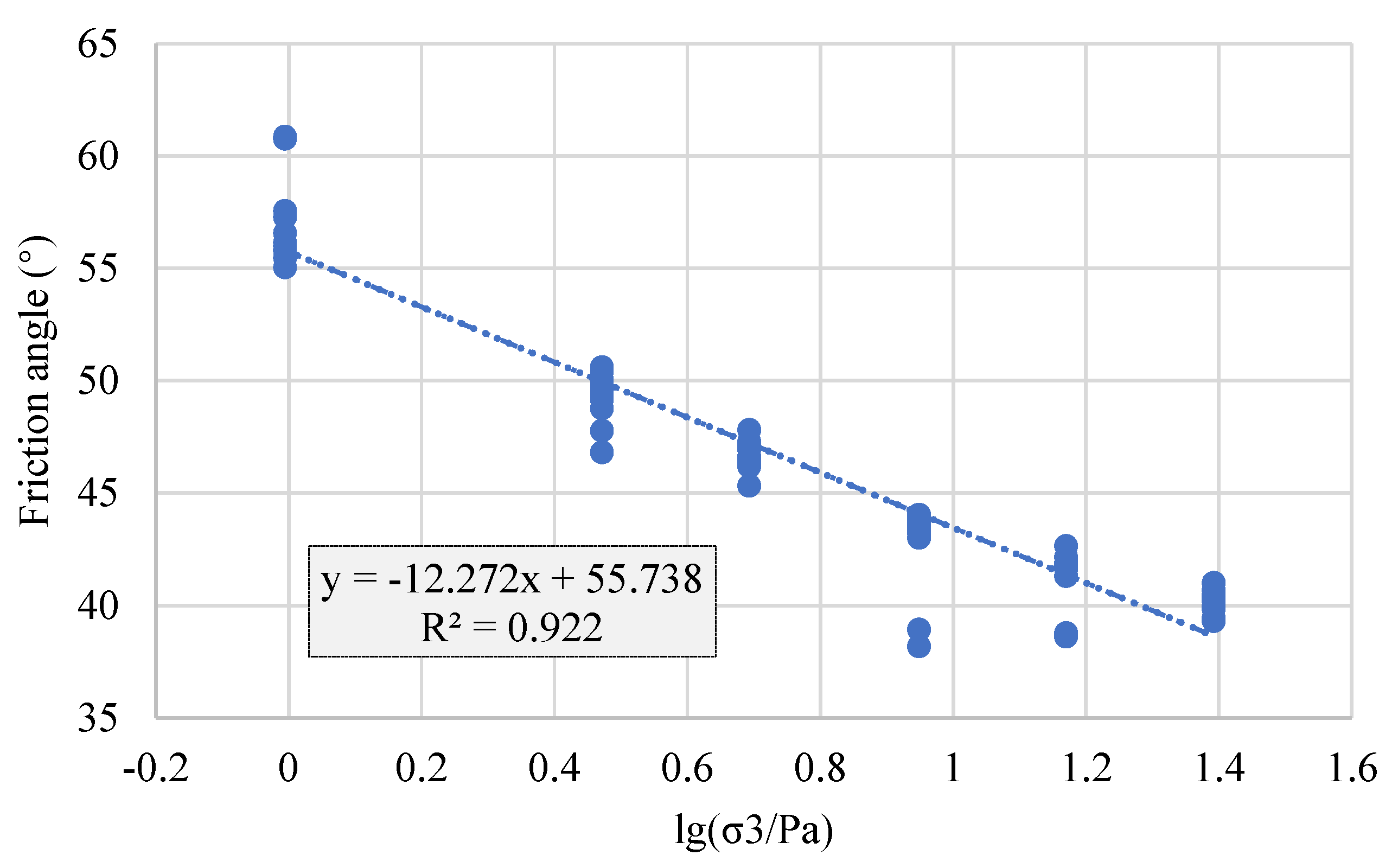
Figure 2.
Regression residuals of nonlinear shear strength and friction angle of coarse-grained soil from Area I of engineering project A from large-scale triaxial tests.
Figure 2.
Regression residuals of nonlinear shear strength and friction angle of coarse-grained soil from Area I of engineering project A from large-scale triaxial tests.
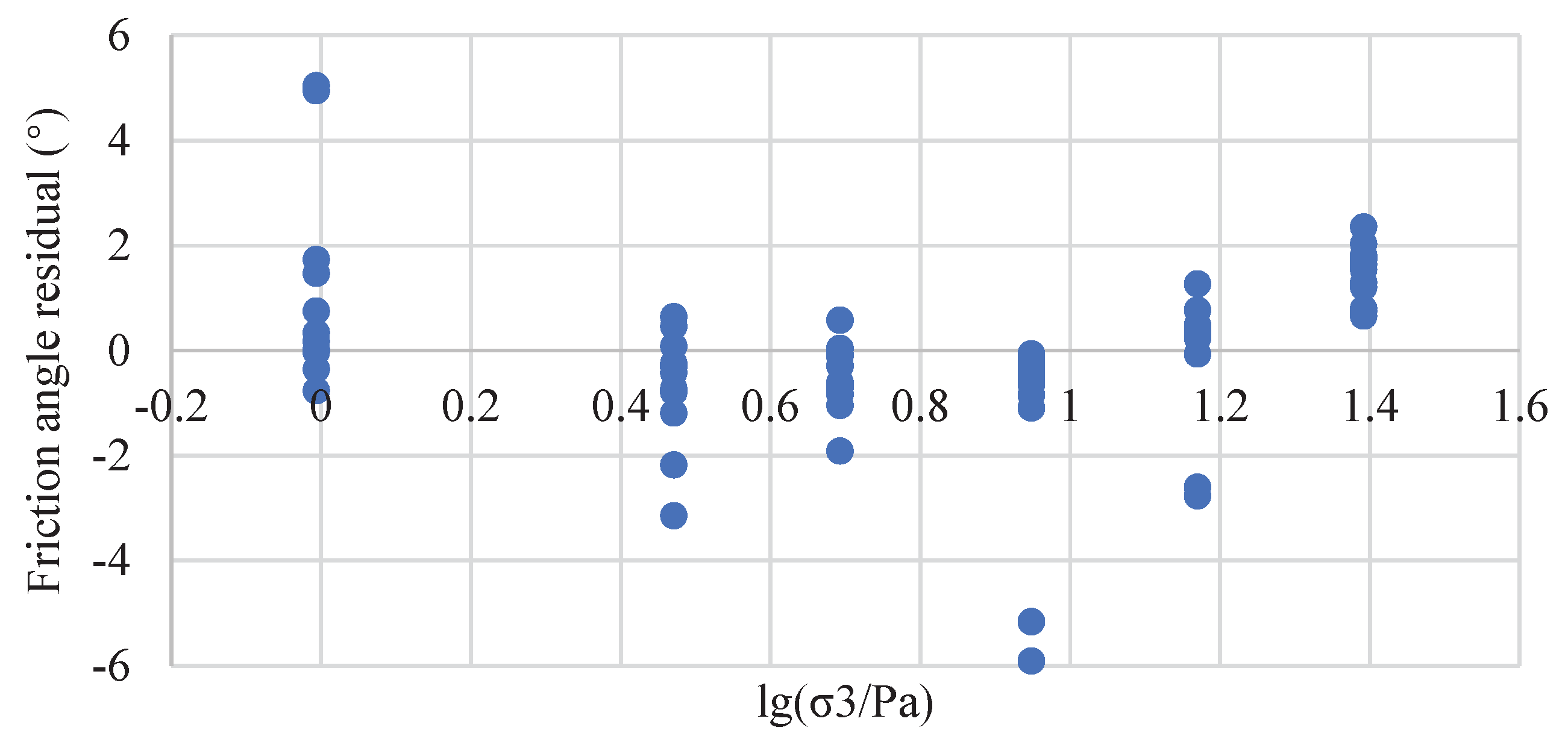

Table 1.
Least squares regression residuals and the residual variances.
| Confining pressure (kPa) | Friction angle residual (°) | Variance | |||||||||||
| 100 | 0.332 | −0.77 | 0.175 | 0.019 | 0.749 | 4.945 | −0.356 | 5.04 | 1.73 | 1.466 | 0.749 | −0.033 | 3.685 |
| 300 | −0.798 | −2.182 | −1.196 | −0.318 | −0.421 | 0.079 | −3.15 | −0.251 | 0.639 | −0.771 | −0.728 | 0.459 | 1.147 |
| 500 | −0.669 | −1.916 | 0.578 | −0.296 | −0.108 | −0.071 | −0.833 | −0.612 | 0.038 | −1.05 | −0.84 | −0.707 | 0.402 |
| 900 | −5.914 | −5.168 | −0.487 | −1.096 | −0.419 | −0.259 | −0.848 | −0.064 | −0.406 | −0.285 | −0.114 | −0.644 | 4.02 |
| 1500 | −2.77 | −2.604 | 0.763 | 0.469 | 0.403 | 0.487 | 0.233 | 0.366 | 0.384 | 1.27 | −0.071 | 0.335 | 1.607 |
| 2500 | 0.653 | 0.794 | 1.757 | 1.2 | 2.026 | 2.355 | 0.746 | 1.814 | 1.544 | 1.728 | 1.293 | 1.629 | 0.286 |
Table 2.
Ratio of variance of least squares regression residuals under different confining pressures.
Table 2.
Ratio of variance of least squares regression residuals under different confining pressures.
| Confining pressure (kPa) | 100 | 300 | 500 | 900 | 1500 | 2500 |
| 100 | 1 | |||||
| 300 |
|
1 | ||||
| 500 |
|
|
1 | |||
| 900 |
|
|
|
1 | ||
| 1500 |
|
|
|
|
1 | |
| 2500 |
|
|
|
|
|
1 |
Note: denotes acceptance of the null hypothesis, denotes rejection of the null hypothesis.
Table 3.
Calculation of R.
| Confining pressure (kPa) | 100 | 300 | 500 | 900 | 1500 | 2500 |
| 100 | 1 | |||||
| 300 | 0.471 | 1 | ||||
| 500 | 0.272 | 0.453 | 1 | |||
| 900 | 0.413 | 0.348 | 0.504 | 1 | ||
| 1500 | 0.337 | 0.323 | 0.537 | 0.957 | 1 | |
| 2500 | 0.67 | 0.616 | 0.555 | 0.704 | 0.69 | 1 |
Table 4.
Calculation of t.
| Confining pressure (kPa) | 100 | 300 | 500 | 900 | 1500 | 2500 |
| 100 | ||||||
| 300 | 1.688/ |
|||||
| 500 | 0.894/ |
1.607/ |
||||
| 900 | 1.434/ |
1.174/ |
1.845/ |
|||
| 1500 | 1.132/ |
1.079/ |
2.013/ |
10.432/ |
||
| 2500 | 2.854/ |
2.473/ |
2.11/ |
3.135/ |
3.015/ |
Note: denotes acceptance of the null hypothesis, denotes rejection of the null hypothesis.
Table 5.
Regression parameters of the Duncan formula for nonlinear shear strength of coarse-grained materials.
Table 5.
Regression parameters of the Duncan formula for nonlinear shear strength of coarse-grained materials.
| Regression method | Regression equation | Covariance matrix | |
| Slightly weathered coarse-grained granite from Area I of the engineering project A | Classic least squares method |
|
|
| Generalized least squares method |
|
|
|
| Coarse aggregate from Area II of engineering project A | Classic least squares method |
|
|
| Generalized least squares method |
|
|
|
| Weathered coarse-grained granite from Area II of engineering project B | Classic least squares method |
|
|
| Generalized least squares method |
|
|
|
| Coarse aggregate from Area II of engineering project B | Classic least squares method |
|
|
| Generalized least squares method |
|
|
|
| Gravel clay material from engineering project C | Classic least squares method |
|
|
| Generalized least squares method |
|
|
Note: The generalized least squares method can eliminate residual variance heteroscedasticity and autocorrelation. Intermediate variables are used to ensure that the regression meets the prerequisites of the least squares method.
Disclaimer/Publisher’s Note: The statements, opinions and data contained in all publications are solely those of the individual author(s) and contributor(s) and not of MDPI and/or the editor(s). MDPI and/or the editor(s) disclaim responsibility for any injury to people or property resulting from any ideas, methods, instructions or products referred to in the content. |
© 2025 by the authors. Licensee MDPI, Basel, Switzerland. This article is an open access article distributed under the terms and conditions of the Creative Commons Attribution (CC BY) license (http://creativecommons.org/licenses/by/4.0/).
Copyright: This open access article is published under a Creative Commons CC BY 4.0 license, which permit the free download, distribution, and reuse, provided that the author and preprint are cited in any reuse.


