Submitted:
01 July 2025
Posted:
02 July 2025
You are already at the latest version
Abstract
Spatial contextual features are effective to inform spatial object detection in terms of the different contextual nature of various objects. Traditional deep neural networks (DNN), such as convolu-tional based networks, only capture part of context by operating window-based convolutions on local neighborhood of pixels in 2D imagery or points in 3D point cloud. However, studies on spatial contextual feature detection on 3D point clouds are limited. This study presents a neural network-based spatial autocorrelation encoder, designed to enhance deep learning-driven 3D geospatial object detection by integrating neural network-derived spatial autocorrelation as a representation of spatial contextual features. The study investigated the effectiveness of such spatial contextual features by estimating the model performance trained on them alone. The results suggested that the derived spatial contextual information can help adequately identify some large objects in an urban-rural scene, such as buildings, terrain, and large trees. We further investigate how the spatial autocorrelation encoder can improve the model performance in terms of geo-spatial object detection. The results demonstrated significant improvements in detection accuracy across varied urban and rural environments, when compared to models without considering the spatial autocorrelation as an ablation. Moreover, the approach also outperformed the models trained by explicitly feeding traditional spatial autocorrelation measures (i.e., Matheron’s semi-variance). This study showcases advantages of the adaptiveness of the neural network-based en-coder in deriving a spatial autocorrelation representation. This advancement bridges the gap between theoretical geospatial concepts and practical AI applications. Consequently, this study demonstrated the potential of integrating geographic theories with deep learning technologies to address challenges in 3D object detection, paving a way for further innovations in this field.
Keywords:
Spatial Autocorrelation
; 3D Point Cloud
; Deep Learning
; GeoAI
; Object Detection
1. Introduction
3D geospatial object detection is underscored in its critical role in building accurate 3D models for state-of-the-art applications of geographic information science (GIScience). These applications span across digital earth [1], twin cities [2,3], and Building Information Modeling (BIM) [4,5], where 3D representations are important not only for visualizing but also for analysis and management of geospatial objects. In the domain of GIScience, the past decades have witnessed a remarkable evolution in 3D techniques, ranging from the development of data acquisition technologies (e.g., RGB-D Camera, and LiDAR1) to the evolution of data processing and analyzing supported by computing technologies. Early studies naively represent 3D spatial objects, essentially reflecting the spatial location of the object in a 3D space. For example, objects were represented by spatial points in a 3D network [6] to describe the spatial relationship among them. Moreover, the representations of buildings are simply derived from blueprints [7,8,9] without the as-built status of them. However, nowadays, the advancements of 3D techniques have made it possible to generate up-to-date and as-is representations of diverse geospatial objects, laying the foundation for the development of 3D geographical information systems (GIS). Therefore, there is a demand for accuracy and efficiency for 3D geospatial object detection.
An illustrative example of this is Tree Folio NYC2, which is a digital twin of New York City (NYC) Urban Canopy produced by the Design Across Scales Lab at Cornell University. It is a web-based GIS application designed to provide practitioners and stakeholders with a user-friendly platform for querying, analyzing, and visualizing the 3D point cloud representations of individual trees in NYC. The development of such applications requires the detection and extraction of trees from 3D point clouds. Due to the number of trees in NYC (approximately 8 million), it would become incredibly time-consuming and labor-intensive work if performed manually.
3D deep learning algorithms can be potentially used to address this challenge. Deep learning for object detection in 3D context has attracted unprecedented attention since the first deep neural network architecture, PointNet [10], which is a deep neural network designed to directly consume point cloud as input, shaping the development of neural network architectures in recent years. The variants of this architecture have been continuously serving as a key part in many cutting-edge architectures from recent studies [11,12,13,14]. Parallel to these advancements, the emergence of GeoAI—a synthesis of GIScience and Artificial Intelligence (AI)—marks a pivotal shift towards not only using cutting-edge AI methodologies to inform geospatial studies but also to enrich AI with geospatial insights [15,16]. A few efforts have been seen since then. For example, Chen [17] conducted a systematic investigation and proved the effectiveness of semivariance as a representation of spatial context in informing 3D deep learning.
Semivariance can be essentially quantified by an approach that evaluates pairwise differences in a neighborhood, such as using Matheron's estimator [18] and Dowd’s estimator [19]. Even though there are enhancement brought by explicitly feeding the semivariance into the model for object detection, there are at least two weaknesses of the method that may entangle the practitioners to use it. One is that pre-calculation of semivariance is required, which demands additional effort towards object detection rather than end-to-end3. The other weakness is that it is difficult for users, especially those without expert knowledge to well configure the parameters, such as number of nearest neighbors, number of bins, and semivariance estimators, which optimal setting might differ for various datasets.
This study tried to advance the efforts toward this thread, which is to explicitly incorporate the spatial context into consideration. Therefore, we proposed a spatial autocorrelation encoder, which is a neural network-based approach to extract high-dimensional vector as a representation of spatial contextual features for the neighborhood of each point based on pairwise differences ordered by spatial lag distance. The proposed neural network-based spatial autocorrelation encoder tries to address the bottlenecks of the previous efforts [17] that explicitly feed pre-calculated semivariance into the model. It neither requires the user to pre-calculate the contextual features for each point, nor demands expert knowledge to carefully configure the dataset-dependent parameters for the model. The proposed encoder automatically extracts a context embedding from the lag-ordered pairwise difference and the parameters are configured during the training process.
The proposed encoder not only enhances the capability of GIS in handling and interpreting 3D geospatial data but also paves the way for further investigation on geospatial insights in benefiting AI models. The implications of this study are significant for various applications, including environmental monitoring, disaster management, and urban studies, where quick and accurate interpretation of spatial data is crucial. The contributions of this study are highlighted as follows:
- Enhanced Geospatial Object Detection by Spatial Context: The study underscores the effectiveness of spatial contextual features for identifying diverse geospatial objects, embracing geographic theories, statistical methods, and deep learning advancements. It demonstrates the pivotal role of spatial statistics in enriching AI technologies for geospatial object detection from complex environments.
- Automate Contextual Representation Extraction: By developing a neural network-based encoder that effectively extracts spatially explicit contextual representations, this research showcases an innovative integration of AI in geospatial analysis. This approach simplifies the application of traditional semivariance estimations, offering a streamlined, and dataset-specific learning mechanism that enhances model accuracy and efficiency in geospatial object detection.
The remainder of this article is organized as follows: Section 2 reviews the related literature with a focus on contextual features in object detection. Section 3 explains the proposed neural network-based encoder for extracting the representation of spatial autocorrelation features. Section 4 demonstrates the 3D point cloud dataset used as an exemplary study case in urban and rural areas. Section 5 outlined our experiments that are designed to investigate the effectiveness of the derived spatial autocorrelation features in informing the model prediction. Moreover, the second experiment serves as an ablation study to verify the usefulness of the proposed neural network-based encoder. Section 6 reports the results of the experiments followed by discussions. Finally, the conclusions are depicted in Section 7.
2. Literature Review
Spatial contexts were identified as an essential features of imagery classification (a.k.a imagery segmentation in the domain of computer vision nowadays) on traditional remotely sensed imagery [20,21,22]. Spatial autocorrelation represented by semivariogram and semivariance are important measures to quantify this phenomenon and have been used for imagery classification in the domain of remote sensing [21,23,24].
Spatial context is also important to the task of 3D object detection [25,26,27]. To improve the performance of deep learning architectures on 3D datasets, many studies focus on using different feature extraction modules to improve the deep learning model. We listed some of them from a scope of geospatial insights enhancing AI model. Wu et al. [12] presented an advanced method for 3D object detection in point clouds, improving upon the Frustum PointNet [28] by incorporating local neighborhood information into point feature computation. This approach enhances the representation of each point through the neighboring features. The novel local correlation-aware embedding operation leads to superior detection performance on the KITTI dataset compared to the F-PointNet baseline. This method emphasized the importance of local spatial relationships for 3D object detection in deep learning frameworks. Klemmer et al. [29] added a positional encoder using Moran’s I as an auxiliary task to enhance a graph neural network in interpolation tasks. Fan et al. [30] designed a module based on the distance between points to capture its local spatial context to inform object detection. Engelmann et al. [27] proposed a neural network to incorporate larger-scale spatial context in order to improve the model performance by considering the interrelationship among subdivisions (i.e., blocks) of the point cloud. While most of the endeavors contribute to improving the model capability to derive discriminative features from spatial information, information from other channels seems to be overlooked [17]. Current LiDAR techniques often capture more information rather than only the position, such as intensity, and RGB, while some special sensors can further collect other spectrum information such as near inferred for thermal studies. Even though some studies integrate RGB as input [10,31,32], colors are not their focus and limited considerations are taken on utilizing them. Chen et al. [17] pioneered a study with a focus on making more use of RGB information by explicitly incorporating semivariance variables to improve the model performance, which are estimated based on the variation of observed color information and corresponding spatial lag distance. Extending the scope of Chen et al. [17], we further explore the spatial variances of non-spatial information in this study. The color information as well as the texture embedded in it, for example, is important for humans to recognize different objects [33,34]. Therefore, we emphasize the importance of color in geospatial object detection. Moreover, we call for an investigation of the channels other than spatial information and corresponding endeavor to improve the performance of models. We are leading a focus shift towards bridging the gap between the development of 3D deep learning and better utilizing non-spatial information.
3. Methodology
3.1. Spatial Autocorrelation and Lag-Ordered Pairwise Differences
Semivariogram is a measure of spatial autocorrelation of a geographic variable. An experimental semivariogram can be represented by a curve consisting of a series of semivariance, , in a lag distance h, where the formula of Matheron’s semivariance [18] can be represented by Equations 1-2.
where Z(xi) is the observed value at the location xi and d is the difference between observed values at xi and xi+h. In the context of 3D LiDAR point cloud, Z(xi) can represent an observed value at the point, such as a color channel value (e.g., RGB values), reflectance at a specific band (e.g., near infrared), and intensity.
In this study, we used the lag-ordered pairwise differences between a point and its neighbors as a representation for spatial autocorrelation-based context. We demonstrate the way to derive lag-ordered pairwise difference using one point as example shown in Figure 1. Let OPD(i,k) represents a set of lag-ordered pairwise differences for a point at location xi and its k-nearest neighbors:
where Δi,j is the absolute value of pairwise differences of xi and a neighbor xj. Δi,j are sorted ascendingly such that the lag distance (h) between xi and xj, :
Data partitioning and subsampling are two essential steps in the preprocessing steps of cutting-edge 3D deep learning methods. This is due to the consideration related to computing resources and the nature of neural networks that the input minibatch needs to be regularized [10]. The point cloud datasets directly collected by sensors such as LiDAR instruments commonly include millions of points with the dataset often at a gigabyte level in size, which is too large to be efficiently or feasibly fed to the CPU and/or GPU [35]. On the other hand, neural networks require structured input, but the unstructured nature of 3D point clouds does not satisfy this requirement. Therefore, we have to perform data partitioning and subsampling to prepare structured and memory-manageable datasets for deep neural networks. These two steps are demonstrated as the first two steps in Figure 1. Data partitioning is implemented by using a particular size of blocks to subtract a subset from the original point cloud. Furthermore, a sampling method is conducted to sample from the subset to an anticipated number. Considering the unevenly distributed nature of 3D point cloud, this step is often done by sampling with replacement. This is to overcome the case that the number of points within the subset does not reach the expected number of points per block.
Defining a neighborhood around a point is a prerequisite to compute pairwise differences. Due to the unstructured nature of a 3D point cloud, it is not feasible to use a fixed distance to identify the neighbors. The number of neighbors within a certain distance can vary across different points. In an extreme scenario, one point in point sparse areas may not find a neighbor within a given distance. Therefore, it is essential to use k nearest neighbor to identify the neighborhood. This idea is supported by many existing studies, such as PointNet++ [31], PointNext [14], and ConvPoint [32] using the kNN approach. kNN is, thus, adopted in this study to identify the neighbors of a point. One argument that is often associated with kNN is that the local neighborhood captured by kNN varied its size for different points, which may lead to inconsistent scales. We are aware of this difficulty brought by kNN that scales as well as features might be inconsistent, but this challenge can be mitigated through random sampling as suggested by Klemmer et al. [29]. Additionally, Boulch [32] suggests that randomly sampling points to represent the same object within the same scene during the training process is a way to mitigate such inconsistencies.
We used tree searching provided by SciPy4 to implement kNN, which is more efficient than calculating all pair distances. Once the k nearest neighbors are identified, the pairwise differences are calculated between the center point (key point) and its neighbors. In the traditional calculation of semivariance, the pairwise differences not only consider pairs between the key point and its neighbors but also all other pairs within the neighborhood. Therefore, the total number of pair differences is n*(n-1). We chose to use the former design because it is not only simpler in computational complexity but also powerful in terms of spatial context representation in our preliminary experiments. Finally, we ordered the k nearest neighbors by its lag distance away from the key points, using this as a representation of initial context features of a point. Subsequently, we applied this approach to all points in the block to prepare a dataset. We chose 16 as the k value to identify the nearest neighbor in this study, referring to the empirical setting from the previous studies when aggregating features from neighbors [30,32].
3.2. Architecture Design of the Spatial Autocorrelation Encoder
Inspired by Chen et al. [17] explicitly feeding semivariance as contextual features for object detection, we aim to automate the estimation process and derive dataset-dependent contextual embeddings by using a spatial autocorrelation encoder5 (see Figure 2). One important requirement for the design of the neural network architecture for 3D deep learning is that the derived representation of point cloud should be permutation invariant to the original input [10]. PointNet uses max pooling as a symmetric function that makes the output global signatures invariant in terms of permutation. ConvPoint [32] adopted a continuous convolution operation to ensure the convoluted features are permutation invariant to the input point cloud. The spatial dependency embeddings extracted by the proposed encoder are naturally permutation invariant to the input point cloud because the input unordered point cloud for the contextual feature estimation will be resorted based on the lag distance.
3.3. Feature Grouping to Embed the Encoder to a Neural Network Architecture
In a deep neural network, each feature extraction layer can extract the features from the previous layer (either input or hidden layers). In such a way, high-level features (from subsequent layers) can be eventually extracted, while the final abstract features should be adequately invariant to most local changes from early layers (e.g., input layer). In our design, we attempt to extract such high-level embedding features from the lag-ordered pairwise differences within a neighborhood and use these features along with embeddings from spatial and color information for the final prediction. The k nearest neighbors were identified for each point, and pairwise differences were estimated based on the values of the neighbors. The lag-ordered pairwise differences were fed into the spatial autocorrelation encoder (see Figure 2).
Aggregating local features to a larger scale (up to global scale, i.e., the entire block of point cloud) can effectively improve the model performance. By incorporating the spatial autocorrelation encoder module, we could concatenate the spatial dependency embeddings with other features at a layer of a neural network. There are three types [31] of grouping approaches (three settings of framework), single-scale point grouping (SSG), multi-scale point grouping (MSG), and multi-resolution point grouping (MRG). SSG is used to extract features in only one scale by layers of neural networks and only uses the final feature map for classification. MRG is extremely computationally expensive [31], in which larger scale features are derived based on features from smaller scale. MSG is a simple but effective approach to group layers from different scales, similar as the idea of skip connections [36]. The final features of points combine features from different scales, where features for each scale can be independently derived. The grouping approaches can also help to mitigate the impact from uneven distribution of point clouds. It is claimed by [27] that MSG is a little higher than SSG in terms of accuracy. Therefore, we followed an MSG approach to group the features. We concatenated the local contextual features with the global and point-wise local features (see Section 5 Experiment 2 for detail).
4. Dataset
Semantic3D, introduced by Hackel et al. [37], stands as a substantial and diverse dataset specifically tailored for outdoor scene analysis. We selected this dataset because its context is close to GIS applications such as digital twins of cities, where it can serve as the original data for 3D modeling geospatial objects, such as buildings, trees, traffic lights, and road surface. The Semantic3D dataset offers a detailed and complex dataset with 15 scenes ranging from urban to rural. It covers a wide range of eight semantic categories, man-made and natural terrains, high and low vegetation, structures such as buildings and hardscape (e.g., road light, and fencing), scanning artefacts (e.g., dynamic noise during scanning), and vehicles (see Figure 3).
As we are moving towards the concept of twin cities, where urban environments are enriched with sensors and technology for better management and planning, the need for accurate and efficient processing of 3D spatial data becomes increasingly critical [1,3]. The ability to accurately segment and interpret this data can inform various aspects of smart city planning, including infrastructure development, environmental monitoring, and emergency response strategies [3,5,6,7,38,39]. The Semantic3D benchmark serves as a bridge between academic research and real-world applications. It provides a common ground for researchers to test and compare their methodologies, fostering an environment of collaboration and continuous improvement. This is particularly important in fast-evolving fields such as GIS, where the gap between theoretical research and practical application needs to be constantly narrowed.
In our methodology, we chose nine of these scenes for our training dataset, selected in terms of the diversity of the scenes (e.g., urban and rural). The remaining six scenes were used for validation to examine the generalization capability of our model. For preprocessing, we adopted an 8-meter block size for dataset partitioning, aligning with recommendations of Boulch [32], and targeted a density of 4,096 points per block. A block size of 8 meters indicates that the dataset is divided by an 8-meter grid, where each block covers an area of 8 meters by 8 meters. This setting is a good rule of thumb for large scale outdoor dataset, which is also supported by [40]. This segmentation facilitates the handling and analysis of large datasets by breaking them down into more manageable units, allowing for detailed processing and analysis of each segment while maintaining the structural nature of spatial data. To maintain the quality of lag-ordered pairwise difference estimation, blocks containing fewer than 128 unique points were excluded. This approach addresses the issue of duplicated points in oversampled blocks by prioritizing unique point locations, ensuring that our model input is not skewed by artificial data replication. For example, when estimating the lag-ordered pairwise differences, only unique points are taken into consideration. Otherwise, oversampled points can count towards k nearest neighbors, which can lead to a weak representation of spatial relationships within the dataset for accurate geospatial object detection.
There are two main challenges in the dataset, uneven point distribution and a long tail problem. The points within these scenes are not uniformly distributed; instead, they exhibit an extremely uneven spatial distribution as the nature of LiDAR data. This unevenness poses a unique challenge as it requires algorithms to be highly adaptable and sensitive to a wide variety of spatial contexts and densities. Furthermore, the classes exhibit extremely uneven distribution, known as a long tail problem. As suggested in Figure 4, the first four largest classes (i.e., building, man-made terrain, high vegetation and natural terrain) represent approximately 90% of the whole dataset. In particular, the building class is approximately 45% of the points in the entire dataset. The remaining four classes, hard scape, low vegetation, cars, and scanning artefacts only represent <10% proportion of the dataset. The ability to adequately represent non-uniform point-cloud data is essential for developing sophisticated 3D deep learning models that can accurately interpret and interact with complex real-world environments. The Semantic3D dataset, therefore, serves as an invaluable resource for advancing research and development in 3D scene analysis and understanding.
5. Experiments
We designed two experiments, where one is to investigate the effectiveness of the proposed encoder with lag-ordered pairwise difference as input for object detection, and the other, served as an ablation study, is to examine how the proposed encoder can inform the 3D deep learning for geospatial object detection.
For the first experiment, we only feed pairwise differences to our proposed encoder following a classification head (see Figure 5). We used the classification head of PointNet here not only because it is concise and powerful to derive good representations [41] but also because of its compatibility to handle any type of input features. Cutting edge architectures have a more sophisticated design requiring an explicit feed of spatial information. For example, neural network architectures designed by [30] have an essential need of explicit spatial information as an input. In this case, we would not be able to explicitly examine the importance of the spatial contextual features, as well as the effectiveness of the proposed encoder with lag-ordered pairwise differences for geospatial object detections.
The other experiment aims to assess the effectiveness of the designed encoder in benefiting the 3D deep learning in terms of object detection (see Figure 6). In addition, we conduct comparative analysis between our results as opposed to those from Chen et al. [17] that uses a combination of spatial information, color information, and/or contextual information.
We conducted model training and validation for each treatment across 10 repetitions to mitigate uncertainties due to the stochastic nature of the training process, where the number was to match that used in [17] to make the results comparable. In this study, Intersection over Union (IoU) is used to measure model performance for each class. The mean Intersection over Union (mIoU), and Overall Accuracy (OA) were adopted to measure the model performance on this dataset as the same as [17]. Consequently, we summarized the average performance measurements over the 10 repetitions. Furthermore, one tailed t-test is applied to examine if their mean values are significantly different. By employing the systematic approach, this experiment aims to offer an in-depth understanding of the effectiveness of the module to inform 3D deep learning. The formulas of the measurements are illustrated as follows:
where i indicate a single class, TP is True Positive (a.k.a hit), FP is False Positive (a.k.a false alarm), and FN is False Negative (a.k.a miss).
6. Results and Discussion
6.1. Investigating Effectiveness of Lag-Ordered Pairwise Difference
Experiment 1 investigated the effectiveness of lag-ordered pairwise differences in terms of geospatial object detection. The measures are reported in Table 1 and demonstration of the results are shown in Figure 7. It is interesting to see that overall accuracy can achieve 63% while the input data is only the lag-ordered pairwise difference without any explicit spatial locations or RGB information, which supports a moderate capability of such features in identifying geospatial objects. The results particularly suggest an adequate performance for identifying those large objects, such as building and high vegetation. This performance is especially visible on selected scenes as shown in Figure 7.
The IoU for each class shows a large difference across classes. The model performance on buildings and high vegetation separately reaches 63% and 54% in terms of IoU. The second tier of classes are man-made terrain and natural terrain, on which the model has an IoU of 39% and 38% correspondingly. The rest of classes, hard scape, low vegetation, cars, and scanning artefacts, are not well detected by the model, leading to the IoU ranging from 0% to 12%.
We observed that the model performance on different classes appears to be related to the proportion of the class within the dataset and the volume of the objects. As shown in Figure 3, buildings, man-made terrain, natural terrain, and high vegetation are the four largest classes, where a cumulative proportion is around 90% of the entire dataset. The model shows better performance on these four classes and appears far better than the rest of classes in terms of IoU. One potential reason that causes the diversity in the performance of the model on each class is the proportion of the class within the dataset. However, it seems it is not only related to the proportion. For example, even though man-made terrain has more points than high vegetation class, the performance on high vegetation is better than that of man-made terrain. It suggests that lag-ordered pairwise differences have the capability to identify different objects while it also appears to be sensitive to the volume of the objects. We attribute this finding to the nature of data partitioning and sampling process. While during this process, the number of points for objects in the original dataset directly impacts how many points from this object can be captured during this process. Moreover, the volume of the object also impacts the analysis. For example, a cubic object (e.g., building and tree) tends to be captured with more points than the planar one since ground only exists on the floor surface of a block but cubic objects exist across the 3D space. Hardscape, scanning artefacts, and cars take a small volume as well as the number of points as opposed to the whole scene. Therefore, they might be less represented using the pairwise differences as the points sampled for them might be more subject to boundary effects.
Even though there are less represented classes, we still innovatively find the capability of lag-ordered pairwise difference as context features to identify many objects. We can tell from Figure 7 that buildings, trees and terrains, even though confusion between natural terrain and man-made terrain, are reasonably identified by the model. The performance of models that utilize spatial information and RGB outperforms the model using only lag-ordered pairwise differences. However, recognizing the utility of pairwise differences remains a significant discovery.
The visualization of the prediction results demonstrated the confusion among classes especially around the boundaries. For example, the natural terrain and man-made terrain are not well distinguished by the model. Moreover, we also observed that some man-made surfaces are predicted as trees if the points are close to a tree. These results represent a challenge of the current method that spatial autocorrelation features of those points on boundaries may not adequately be represented since the neighboring points can come from other classes. This problem is also seen in the classification task on 2D remotely sensed imagery when spatial autocorrelation is considered. Myint [42] attempted to mitigate this challenge by excluding the samples on the boundaries during model training. Wu et al. [24] addressed the boundary issue by considering the object-based spatial contextual features instead of the window-based one. However, further study has to be conducted to adapt these solutions from 2D to 3D context so that this challenge can be well addressed.
6.2. Performance of Spatial Autocorrelation Encoder
Experiment 2 investigates the effectiveness of the designed spatial autocorrelation encoder through a ablation study along with results from Chen et al. [17] in which the two experiments from Chen’s study served as the two without such neural network-based spatial autocorrelation encoder. In this section we demonstrated the measurement statistics across the 10 repetitions (see detail in Appendix A) in Table 2. We further demonstrate our results in Figure 8 comparing with the results without using the encoder.
The OA, and mIOU are 85.5%, and 57.6% separately, providing a global measure for the model performance for this dataset. The IoU across the classes ranges from 26.8% (scanning artefacts) to 92.8% (man-made terrain). The same as reflected in Experiment 1, the classes with higher proportion from the original datasets tend to have a better performance. For example, man-made terrain (IoU 92.8%), buildings (IoU 84.0%), natural terrain (IoU 78.7%), and high vegetation (IoU 66.1%) are the four classes that the model best performed on, while they are also the four largest classes with a cumulative proportion of 90% of the original dataset. We attribute their better performance to the amount of data compared to the rest of the classes. The model shows a moderate performance on cars with 55.6% IoU. Scanning artefacts, hard scape, and low vegetation seem to be not well detected by the model with IoU ranging from 26.8% to 28.8%.
6.3. Comparative Analysis
We conducted a comparative analysis between the results from our study with those from Chen [17]. Chen [17] analyzed how the input feature will impact the model performance on geospatial object detection, where the three treatments are spatial information only, spatial information and RGB, and one with additional semivariances. It has been shown that the latter two produced a significant increase in accuracy as compared to the use of spatial information on its own. In this analysis, we compare our results with those from Chen [17] for treatments including RGB and additionally combining semivariances. We use RGB as a baseline to investigate how context information can inform the model for geospatial object detection and one tailed t-test is performed against the baseline to explore its statistical significance (see Table 3).
For the global measurements, OA, and mIOU, there is an increasing trend in accuracy as we consider spatial context with more sophisticated measures. Without considering the spatial content, the three measurements are 81.95%, 64.03%, and 51.58% using RGB data on its own. Explicitly incorporating semivariance as a spatial context feature can result in a 1-3% increase in the global measurements. Once we applied a neural network to directly learn a spatial context embedding from lag-ordered pairwise differences, accuracy improved 3.60%, 4.69%, and 6.00% for the three assessment measures with the increase being significant at a 99% confidence interval.
Comparative analysis significantly underscores the advancement our study brings to the field of geospatial object detection using 3D deep learning. By directly learning spatial context embeddings from lag-ordered pairwise differences, our approach outperforms previous models trained on RGB and/or semivariance in terms of OA and mIOU. The substantial gains across various classes, particularly in categories such as high vegetation and cars, highlight the effectiveness of incorporating spatial autocorrelation features. The comparative results validate the advancement of the proposed encoder-based neural network approach over previous approaches in deriving spatial contextual features in geospatial object detection tasks. The statistical significance of these results emphasizes the critical role of spatial contextual features in enhancing 3D deep learning models, paving the way for future advancements in this rapidly evolving field.
7. Conclusions
This study introduces a neural network-based spatial autocorrelation encoder to integrate spatial contextual features into 3D deep learning of geospatial object detection. By leveraging lag-ordered pairwise differences, the encoder-based neural network approach significantly improves the accuracy of geospatial object detection, especially in urban and natural environments. Experimental results demonstrate the effectiveness of this approach, suggesting its potential for a wide range of applications in urban studies, transportation and infrastructure, and environmental studies. Moreover, it also highlights the effectiveness of spatial autocorrelation in informing geospatial object detection, which can contribute to model capability in terms of differentiating geospatial objects. This finding is innovative and suggests the potential use of pairwise differences in future improvements in geospatial object detection. Furthermore, the proposed spatial autocorrelation encoder not only streamlines the workflow for geospatial object detection explicitly considering spatial autocorrelation but also simplifies the extraction of sophisticated spatial autocorrelation features, making it accessible to practitioners without expertise in the field.
Our study started initially from the call for integrating GIS, and AI to enhance the development of state-of-the-art GIS applications, such as digital twin projects. By innovating in the realm of geospatial object detection, our study provides a foundation for future research and applications in urban studies, environmental monitoring, and beyond. The exploration and findings presented serve not only as remarkable progress witnessed in these domains but also as a bridge connecting the theoretical underpinnings of GIS with the practical applications of AI in 3D geospatial object detection.
Author Contributions
Conceptualization, T.C., and W.T.; methodology, T.C.; software, T.C.; validation,T.C.; formal analysis, T.C.; investigation, T.C.; resources, T.C., W.T., S.C., and C.A.; data curation, T.C.; writing—original draft preparation, T.C.; writing—review and editing, T.C., W.T., S.C., and C.A.; visualization, T.C.; supervision, W.T. All authors have read and agreed to the published version of the manuscript.
Data Availability Statement
The dataset is available at https://www.semantic3d.net/
Conflicts of Interest
The authors declare no conflicts of interest.
Appendix A. Inference Performance of 10 Repetitions
| Treat | OA | mIoU | Man-made terrain | Natural terrain | High vegetation | Low vegetation | Buildings | Hardscape | Scanning artefacts |
| 1 | 85.7% | 57.7% | 93.0% | 79.6% | 67.0% | 28.4% | 84.3% | 28.3% | 26.4% |
| 2 | 85.6% | 57.3% | 92.5% | 78.8% | 66.2% | 28.3% | 84.1% | 28.9% | 25.2% |
| 3 | 85.8% | 58.4% | 92.8% | 80.4% | 66.8% | 29.7% | 84.4% | 28.3% | 26.9% |
| 4 | 85.6% | 57.5% | 92.8% | 78.4% | 66.5% | 25.8% | 84.0% | 27.2% | 28.6% |
| 5 | 85.3% | 57.4% | 92.7% | 76.4% | 66.3% | 25.7% | 83.8% | 27.6% | 29.0% |
| 6 | 85.4% | 56.9% | 92.4% | 78.0% | 68.3% | 25.7% | 84.7% | 26.1% | 27.4% |
| 7 | 85.4% | 57.6% | 92.8% | 77.3% | 63.9% | 31.2% | 84.2% | 28.3% | 27.0% |
| 8 | 85.1% | 57.1% | 92.5% | 77.2% | 66.0% | 29.4% | 83.8% | 26.5% | 25.8% |
| 9 | 85.8% | 58.0% | 93.1% | 80.4% | 64.8% | 33.2% | 83.0% | 28.3% | 23.9% |
| 10 | 85.7% | 57.9% | 93.1% | 80.2% | 65.4% | 30.8% | 84.1% | 28.0% | 28.1% |
| *Treat is for treatment IDs. *OA and mIoU: Overall Accuracy and mean Intersection over Union. The class label: Intersection over Union for each category. | |||||||||
| 1 | LiDAR stands for light detection and ranging. |
| 2 | A digital twin of New York City’s Urban Canopy. Link: https://labs.aap.cornell.edu/daslab/projects/treefolio
|
| 3 | End-to-end, in the domain machine learning, typically refers to a process or a model that takes raw data as input and directly produces the expected output, without demanding any manual intermediate steps operated by humans. |
| 4 | |
| 5 | Encoder is a module from a neural network to extract features and generate a representation of input data. See Klemmer, Safir and Neill (2023) as an example. |
References
- Guo, H., Goodchild, M., and Annoni, A., Manual of digital Earth. 2020: Springer Nature.
- Goodchild, M.F., Elements of an infrastructure for big urban data. Urban Informatics, 2022. 1(1): p. 3. [CrossRef]
- Batty, M., Digital Twins in City Planning. Nature Computational Science, 2023. 4(3). [CrossRef]
- Goodchild, M.F., Introduction to urban big data infrastructure. Urban Informatics, 2021: p. 543-545.
- Batty, M., Agents, Models, and Geodesign. 2013.
- Kwan, M.-P. and Lee, J., Emergency response after 9/11: The potential of real-time 3D GIS for quick emergency response in micro-spatial environments. Computers, Environment and Urban Systems, 2005. 29(2): p. 93-113.
- Evans, S., Hudson-Smith, A., and Batty, M., 3-D GIS: Virtual London and beyond. An exploration of the 3-D GIS experience involved in the creation of virtual London. Cybergeo: European Journal of Geography, 2006.
- Batty, M. and Hudson-Smith, A., Urban simulacra: London. Architectural Design, 2005. 75(178): p. 42-47. [CrossRef]
- Batty, M., The new urban geography of the third dimension. Environment and Planning B-Planning & Design, 2000. 27(4): p. 483-484. [CrossRef]
- Qi, C., Su, H., Mo, K., and Guibas, L.J. Pointnet: Deep learning on point sets for 3d classification and segmentation. in Proceedings of the IEEE conference on computer vision and pattern recognition. 2017.
- Xie, J., Xu, Y., Zheng, Z., Zhu, S.-C., and Wu, Y.N. Generative pointnet: Deep energy-based learning on unordered point sets for 3d generation, reconstruction and classification. in Proceedings of the IEEE/CVF Conference on Computer Vision and Pattern Recognition. 2021.
- Wu, C., Pfrommer, J., Beyerer, J., Li, K., and Neubert, B. Object detection in 3D point clouds via local correlation-aware point embedding. in 2020 Joint 9th International Conference on Informatics, Electronics & Vision (ICIEV) and 2020 4th International Conference on Imaging, Vision & Pattern Recognition (icIVPR). 2020. IEEE.
- Ren, D., Ma, Z., Chen, Y., Peng, W., Liu, X., Zhang, Y., and Guo, Y., Spiking PointNet: Spiking neural networks for point clouds. Advances in Neural Information Processing Systems, 2024. 36.
- Qian, G.C., Li, Y.C., Peng, H.W., Mai, J.J., Hammoud, H.A.A.K., Elhoseiny, M., and Ghanem, B., PointNeXt: Revisiting PointNet plus plus with Improved Training and Scaling Strategies. Advances in Neural Information Processing Systems 35, Neurips 2022, 2022. 35: p. 23192-23204.
- Goodchild, M.F., The Openshaw effect. International Journal of Geographical Information Science, 2022. 36(9): p. 1697-1698.
- Li, W., GeoAI and Deep Learning. The International Encyclopedia of Geography., 2021: p. 1-6.
- Chen, T., Tang, W., Allan, C., and Chen, S.-E., Explicit Incorporation of Spatial Autocorrelation in 3D Deep Learning for Geospatial Object Detection. Annals of the American Association of Geographers, 2024. 114(10): p. 2297-2316. [CrossRef]
- Matheron, G., Principles of geostatistics. Economic Geology, 1963. 58(8): p. 1246-1266. [CrossRef]
- Dowd, P.A., The Variogram and Kriging: Robust and Resistant Estimators, in Geostatistics for Natural Resources Characterization, G. Verly, et al., Editors. 1984, Springer Netherlands: Dordrecht. p. 91-106.
- Miranda, F.P. and Carr, J.R., Application of the semivariogram textural classifier (STC) for vegetation discrimination using SIR-B data of the guiana shield, northwestern brazil. Remote Sens. Rev., 1994. 10(1-3): p. 155-168.
- Miranda, F.P., Fonseca, L.E.N., and Carr, J.R., Semivariogram textural classification of JERS-1 (Fuyo-1) SAR data obtained over a flooded area of the Amazon rainforest. Int. J. Remote Sens., 1998. 19(3): p. 549-556. [CrossRef]
- Miranda, F.P., Fonseca, L.E.N., Carr, J.R., and Taranik, J.V., Analysis of JERS-1 (Fuyo-1) SAR data for vegetation discrimination in northwestern Brazil using the semivariogram textural classifier (STC). Int. J. Remote Sens., 1996. 17(17): p. 3523-3529. [CrossRef]
- Miranda, F.P., Macdonald, J.A., and Carr, J.R., Application of the semivariogram textural classifier (STC) for vegetation discrimination using SIR-B data of Borneo. Int. J. Remote Sens., 1992. 13(12): p. 2349-2354. [CrossRef]
- Wu, X., Peng, J., Shan, J., and Cui, W., Evaluation of semivariogram features for object-based image classification. Geo-spatial Information Science, 2015. 18(4): p. 159-170. [CrossRef]
- Mottaghi, R., Chen, X., Liu, X., Cho, N.-G., Lee, S.-W., Fidler, S., Urtasun, R., and Yuille, A. The role of context for object detection and semantic segmentation in the wild. in Proceedings of the IEEE Conference on Computer Vision and Pattern Recognition. 2014.
- Pohlen, T., Hermans, A., Mathias, M., and Leibe, B. Full-resolution residual networks for semantic segmentation in street scenes. in Proceedings of the IEEE Conference on Computer Vision and Pattern Recognition. 2017.
- Engelmann, F., Kontogianni, T., Hermans, A., and Leibe, B. Exploring spatial context for 3D semantic segmentation of point clouds. in Proceedings of the IEEE international conference on computer vision workshops. 2017.
- Charles, R.Q., Liu, W., Wu, C., Su, H., and Leonidas, J.G. Frustum pointnets for 3D object detection from RGB-D data. in Proceedings of the IEEE conference on computer vision and pattern recognition. 2018.
- Klemmer, K., Safir, N.S., and Neill, D.B. Positional encoder graph neural networks for geographic data. in International Conference on Artificial Intelligence and Statistics. 2023. PMLR.
- Fan, S., Dong, Q., Zhu, F., Lv, Y., Ye, P., and Wang, F.-Y., SCF-net: Learning spatial contextual features for large-scale point cloud segmentation, in 2021 IEEE/CVF Conference on Computer Vision and Pattern Recognition (CVPR). 2021, IEEE. p. 14504-14513.
- Qi, C.R., Yi, L., Su, H., and Guibas, L.J., PointNet plus plus : Deep Hierarchical Feature Learning on Point Sets in a Metric Space. Advances in Neural Information Processing Systems 30 (Nips 2017), 2017. 30.
- Boulch, A., ConvPoint: Continuous convolutions for point cloud processing. Computers & Graphics-Uk, 2020. 88: p. 24-34. [CrossRef]
- Haralick, R.M., Shanmugam, K., and Dinstein, I., Textural Features for Image Classification. Ieee Transactions on Systems Man and Cybernetics, 1973. Smc3(6): p. 610-621.
- Tso, B. and Olsen, R.C., Scene classification using combined spectral, textural and contextual information. Algorithms and Technologies for Multispectral, Hyperspectral, and Ultraspectral Imagery X, 2004. 5425: p. 135-146.
- Li, Z., Hodgson, M.E., and Li, W., A general-purpose framework for parallel processing of large-scale LiDAR data. International Journal of Digital Earth, 2018. 11(1): p. 26-47. [CrossRef]
- He, K., Zhang, X., Ren, S., and Sun, J. Deep residual learning for image recognition. in Proceedings of the IEEE conference on computer vision and pattern recognition. 2016.
- Hackel, T., Savinov, N., Ladicky, L., Wegner, J.D., Schindler, K., and Pollefeys, M., Semantic3D.net: A new large-scale point cloud classification benchmark. ISPRS Annals of the Photogrammetry, Remote Sensing and Spatial Information Sciences. Vol. IV-1-W1. 2017. [CrossRef]
- Li, W., Batty, M., and Goodchild, M.F., Real-time GIS for smart cities. International Journal of Geographical Information Science, 2020. 34(2): p. 311-324.
- Batty, M., Virtual Reality in Geographic Information Systems. Handbook of Geographic Information Science, 2008: p. 317-334.
- Tang, W., Chen, S.-E., Diemer, J., Allan, C., Chen, T., Slocum, Z., Shukla, T., Chavan, V.S., and Shanmugam, N.S., DeepHyd: A deep learning-based artificial intelligence approach for the automated classification of hydraulic structures from LiDAR and sonar data. 2022, North Carolina Department of Transportation. Research and Development Unit.
- Guo, Y., Wang, H., Hu, Q., Liu, H., Liu, L., and Bennamoun, M., Deep Learning for 3D Point Clouds: A Survey. IEEE Trans Pattern Anal Mach Intell, 2021. 43(12): p. 4338-4364. [CrossRef]
- Myint, S.W., Fractal approaches in texture analysis and classification of remotely sensed data: comparisons with spatial autocorrelation techniques and simple descriptive statistics. International Journal of Remote Sensing, 2003. 24(9): p. 1925-1947. [CrossRef]
Figure 1.
Illustration of deriving lag-ordered pairwise differences for a single point and its neighbors. Data partitioning with blocks and sampling are the steps for preprocessing training data for deep learning-based 3D point cloud classification to regularize the input. The set of differences are sorted ascendingly by lag distance from nearby to distant pairs.
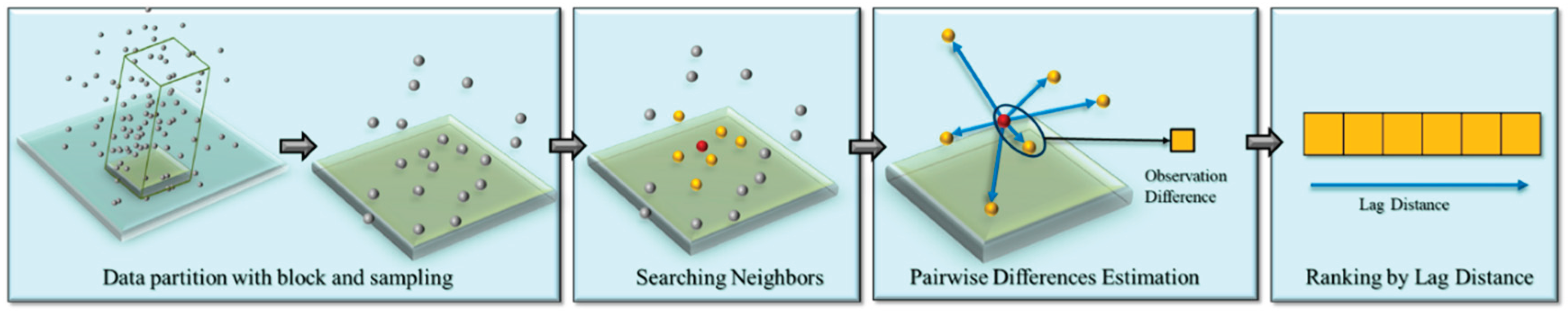
Figure 2.
Proposed spatial autocorrelation encoder for spatial autocorrelation features extraction using deep learning. The multi-layer perceptron shared weights along the rows, which is equivalent to a 1-dimensional convolutional layer (see examples in [10,31]). The numbers in parenthesis are the number of input channels, the number of neurons in hidden layers, and # output channels.
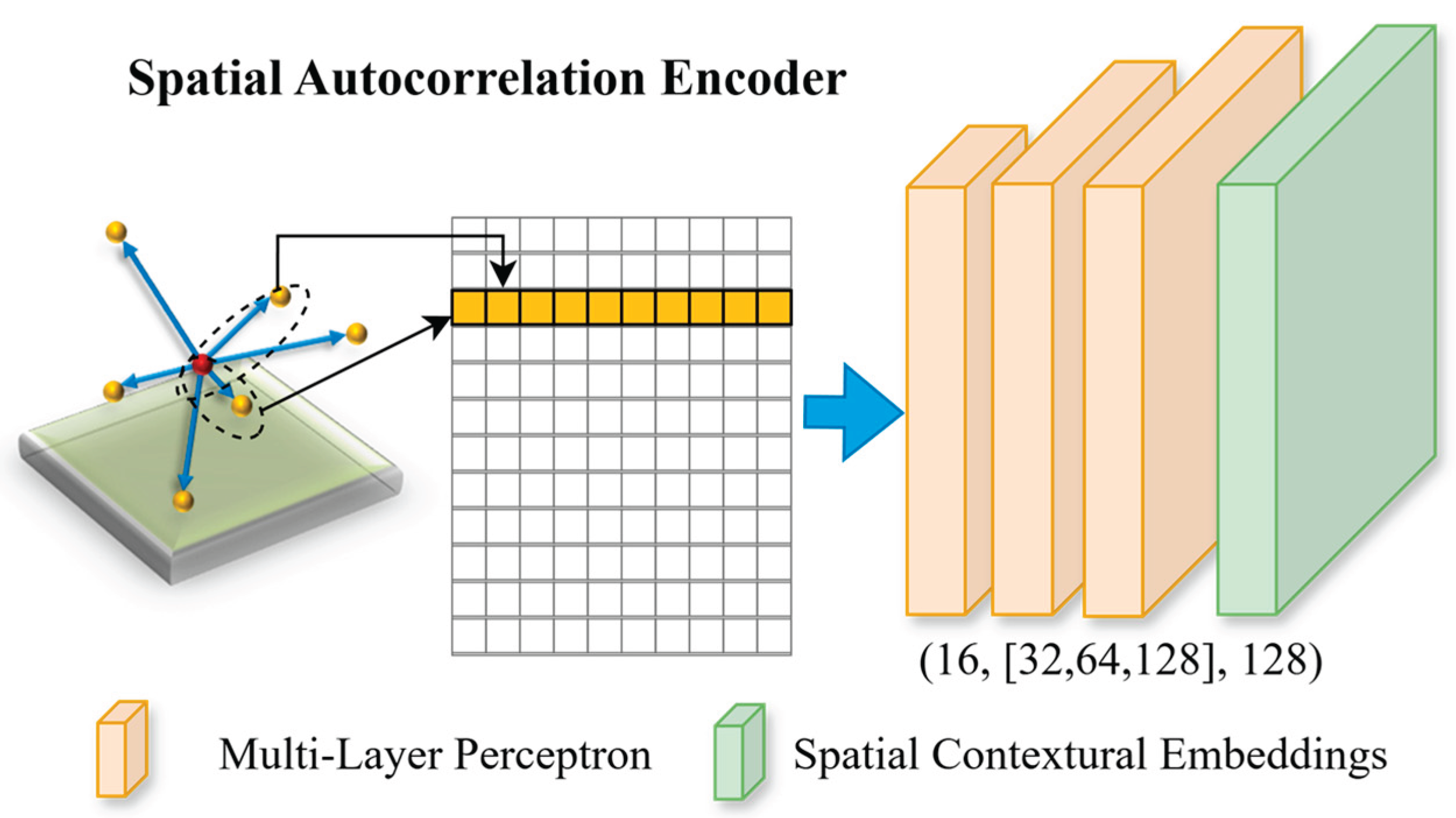
Figure 3.
Illustration of Semantic3D benchmark dataset for urban and rural areas. The first row is the raw LiDAR point cloud with RGB color. The last row shows the labels with discriminative colors for the scenes accordingly. The middle rows are a zoom-in scope of the scenes with LiDAR point cloud and labels.
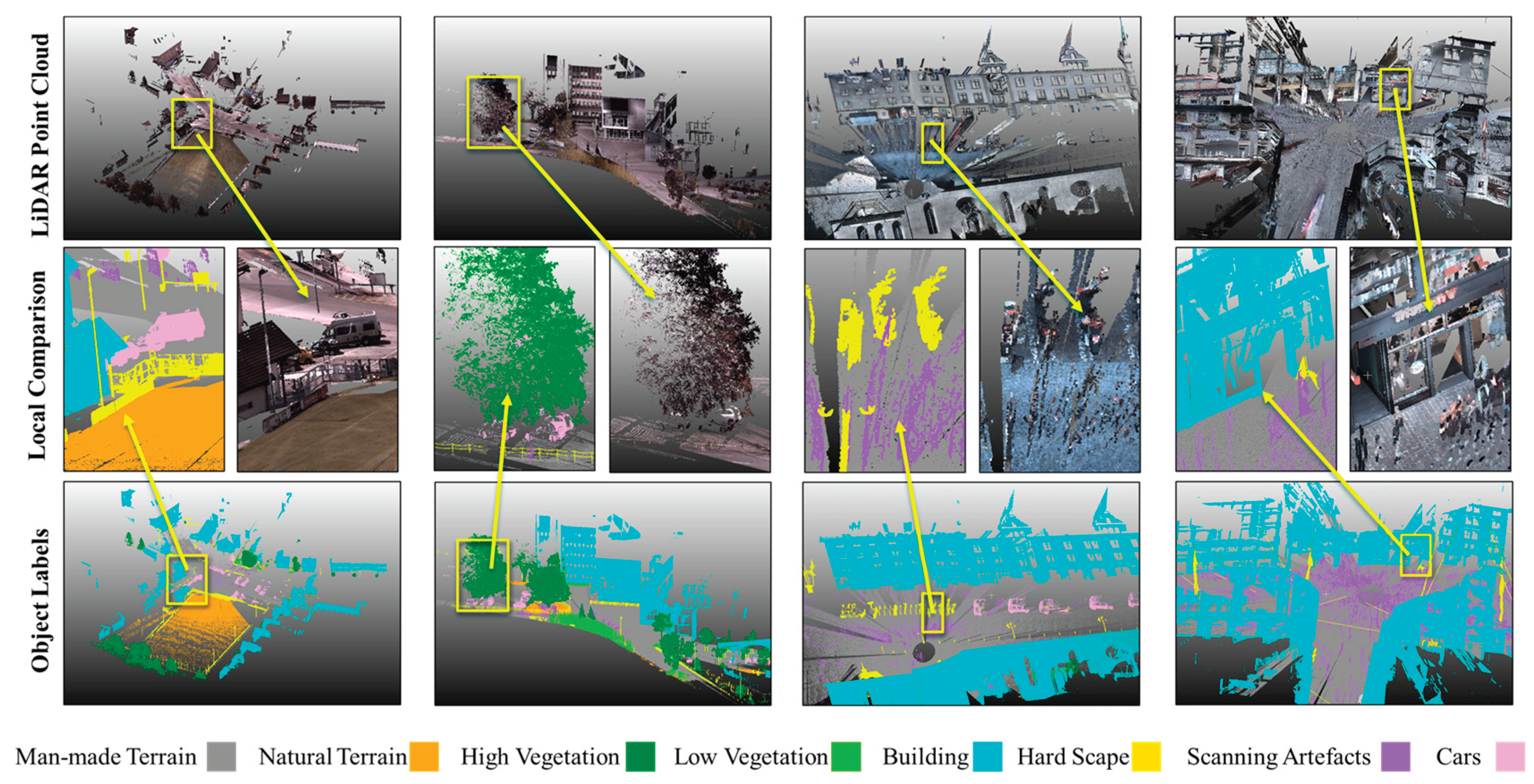
Figure 4.
Distribution of different classes in Semantic3D dataset. The classes are imbalanced in terms of the number of points. A long tail problem can be seen that buildings, terrains, and high vegetation are dominant classes. Cars and scanning artefacts are minor classes.
Figure 4.
Distribution of different classes in Semantic3D dataset. The classes are imbalanced in terms of the number of points. A long tail problem can be seen that buildings, terrains, and high vegetation are dominant classes. Cars and scanning artefacts are minor classes.
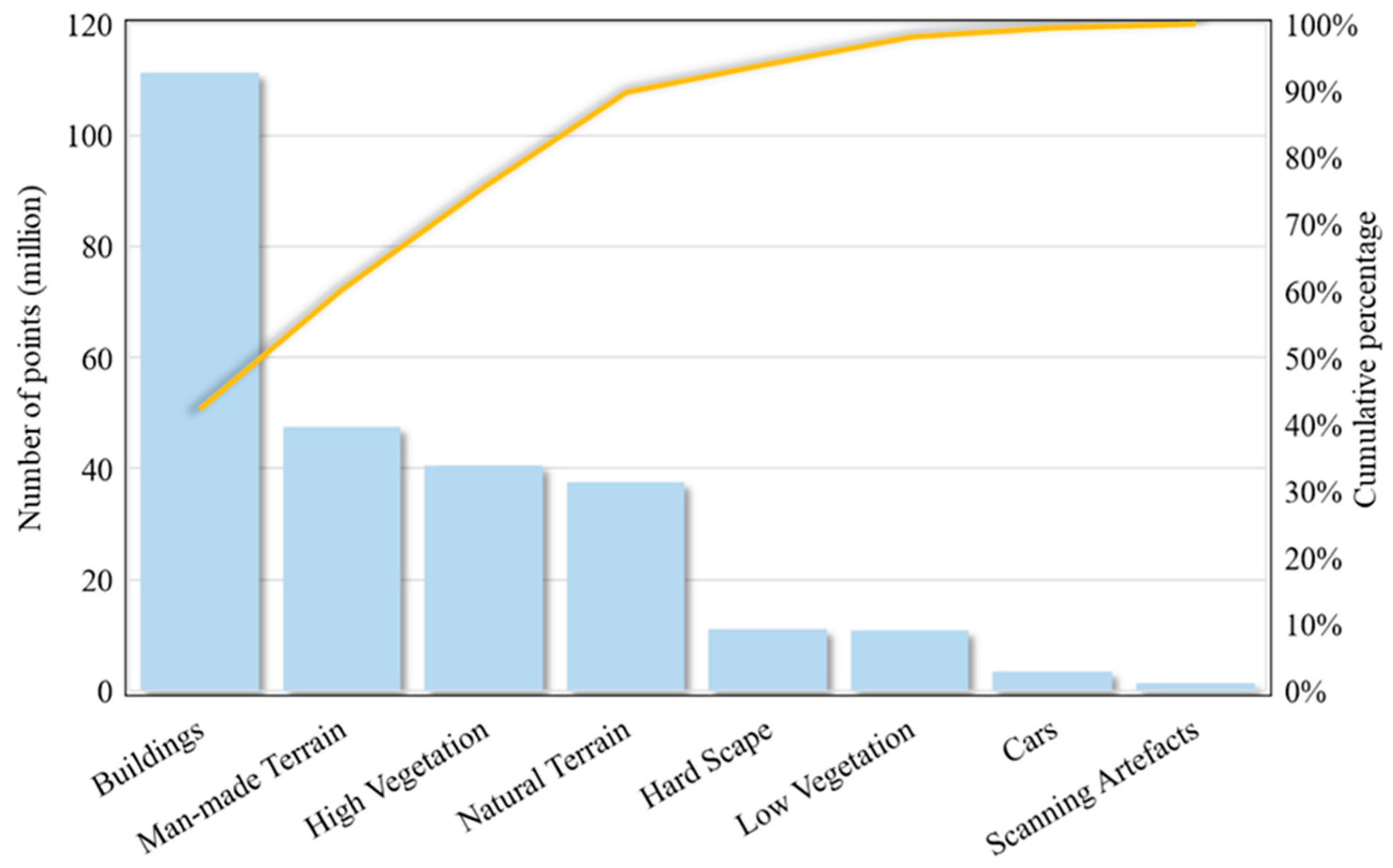
Figure 5.
Deep neural network architecture in Experiment 1 to examine the effectiveness of the spatial autocorrelation encoder as well as the effectiveness of the derived spatial contextual embeddings in informing 3D geospatial object detection. The multi-layer perceptron shared weights along the rows, which is equivalent to a 1-dimensional convolutional layer (see examples in [10,31]). The numbers in parenthesis are the number of input channels, the number of neurons in hidden layers, and # output channels.
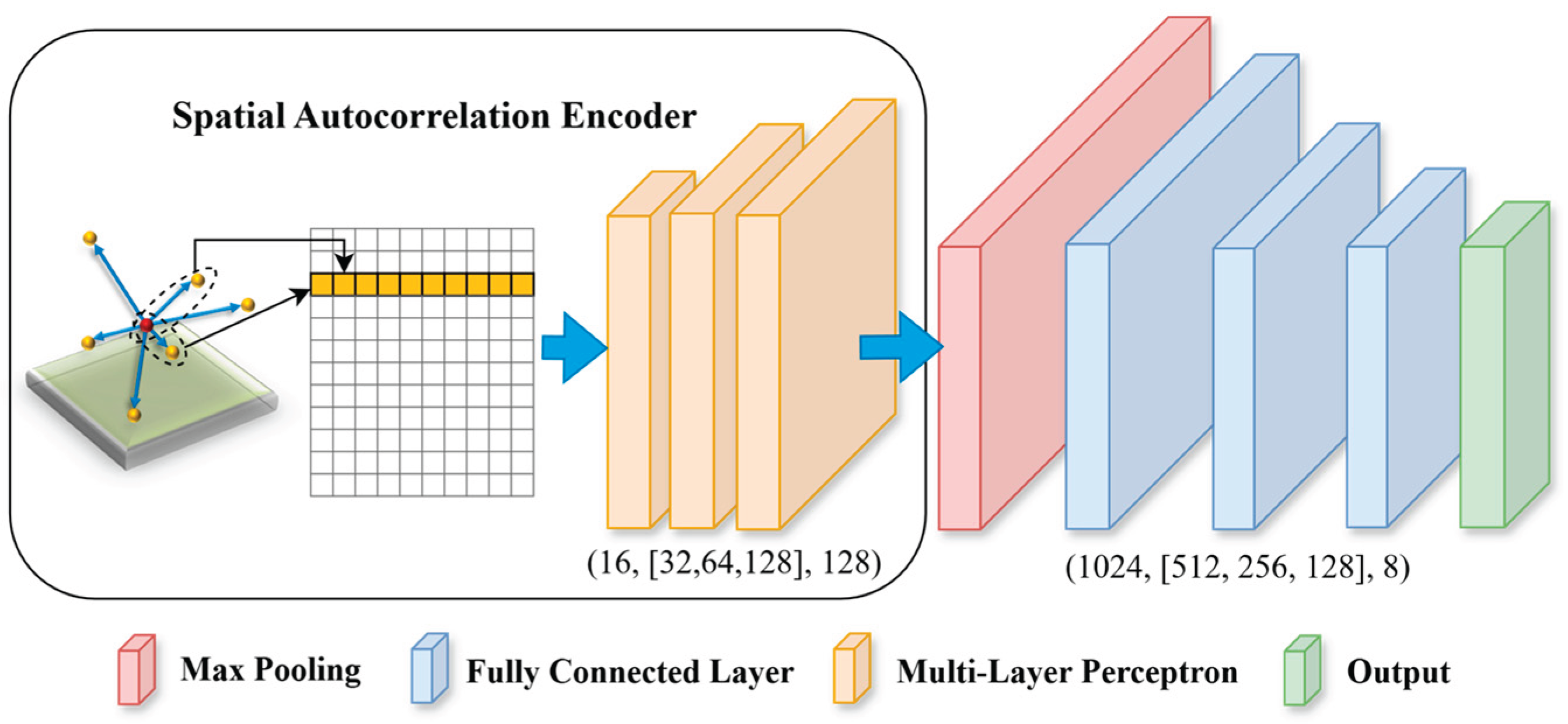
Figure 6.
Demonstration of deep neural network architecture used in Experiment 2. The model performance are compared with the study [17] using the same architecture shown at bottom without the proposed encoder. The multi-layer perceptron shared weights along the rows, which is equivalent to a 1-dimensional convolutional layer (see examples in [10,31]). The numbers in parenthesis are the number of input channels, the number of neurons in hidden layers, and # output channels.
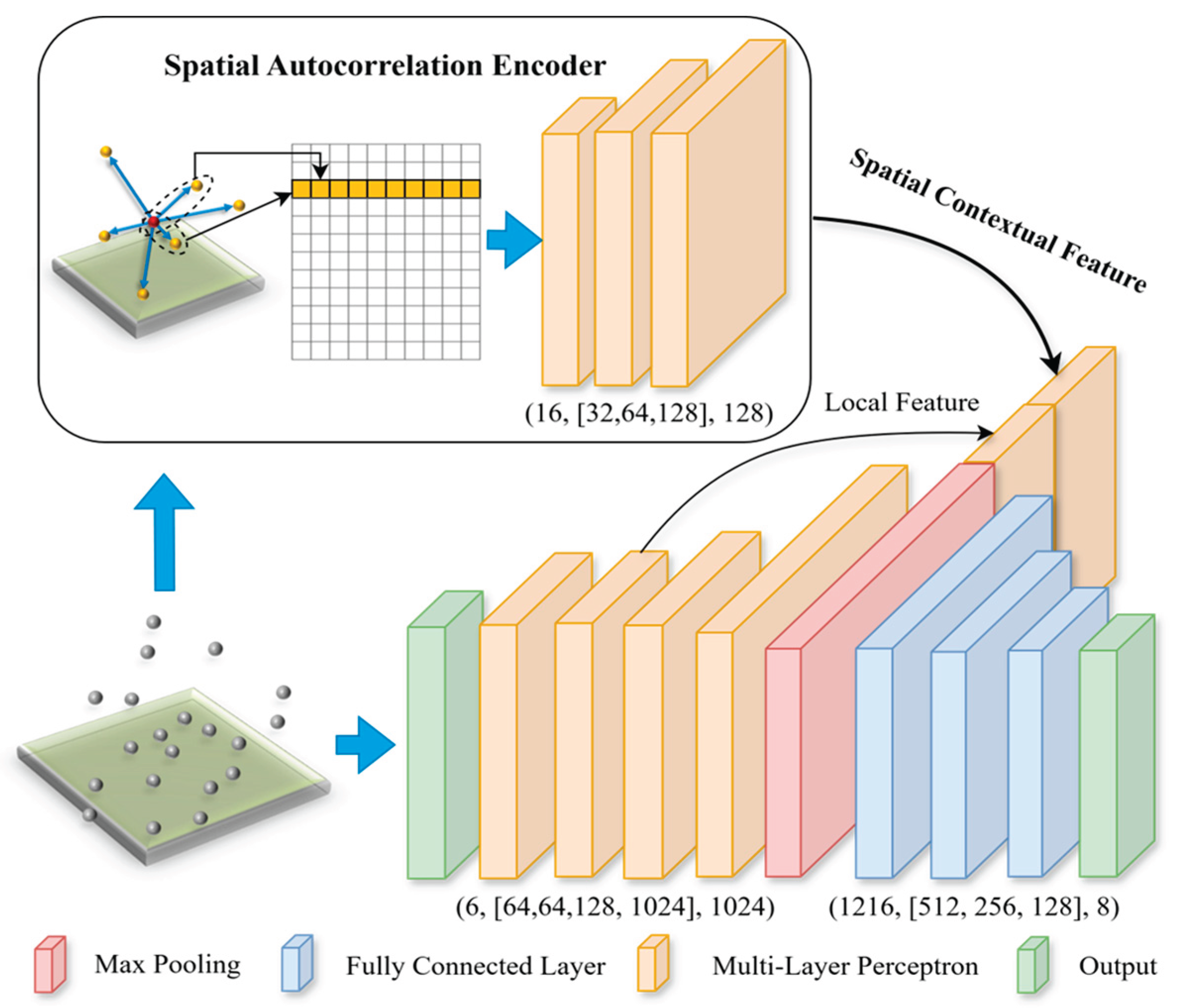
Figure 7.
Visualization of the prediction results on two example scenes using Lag-ordered pairwise differences only as the input. Lag-ordered pairwise differences only show an adequate performance on objects with a large volume in the scene, such as high vegetation, natural/man-made terrain, and buildings.
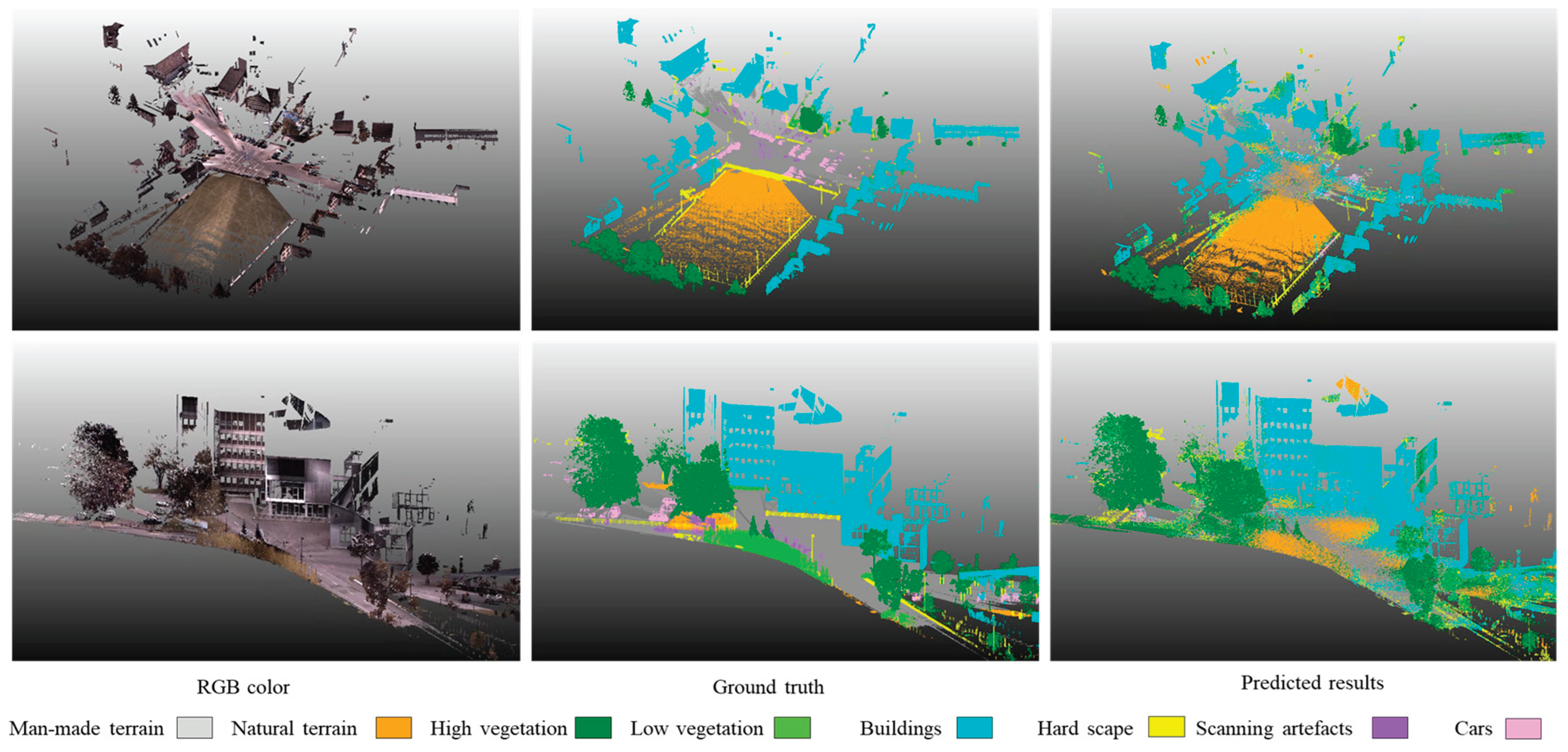
Figure 8.
Comparison between ground truth, and the predicted results with/without spatial autocorrelation encoder on two example scenes.
Figure 8.
Comparison between ground truth, and the predicted results with/without spatial autocorrelation encoder on two example scenes.
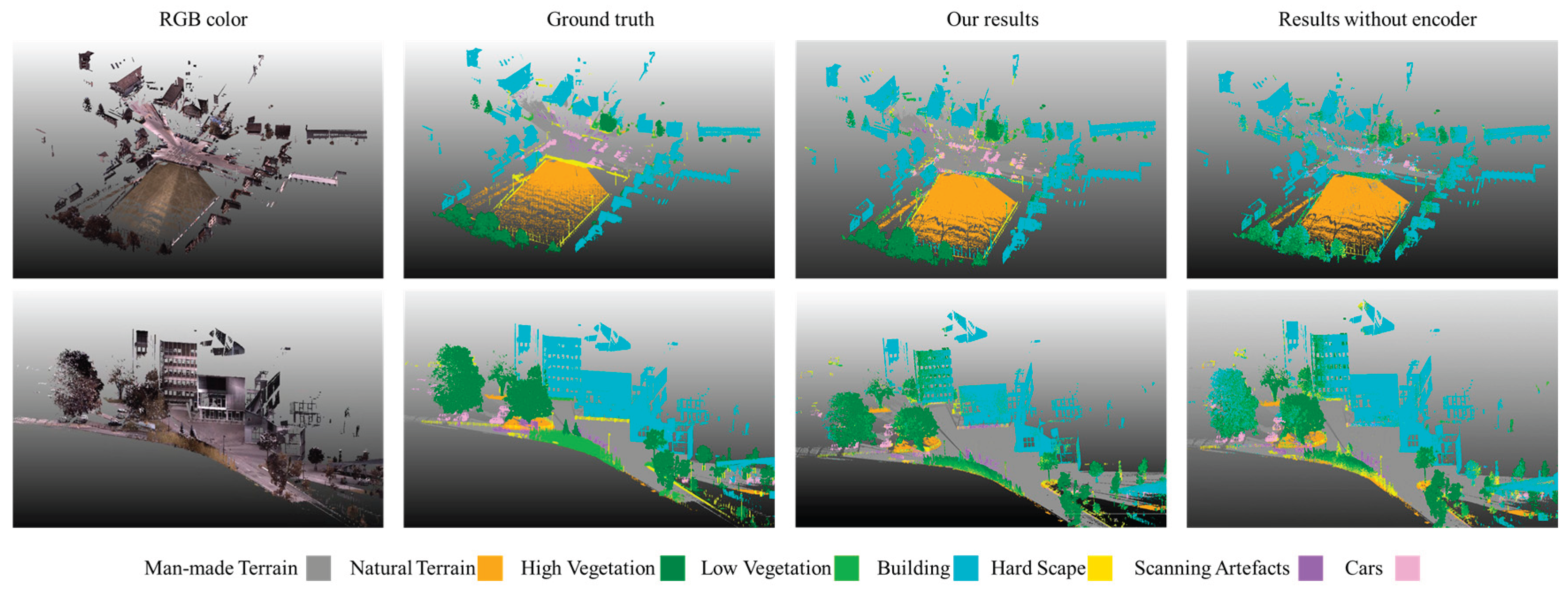

Table 1.
Performance results for Experiment 1 averaged across repetitions.
| OA | 63% |
| mIOU | 28% |
| Man-made terrain | 39% |
| Natural terrain | 38% |
| High vegetation | 54% |
| Low vegetation | 8% |
| Buildings | 63% |
| Hard scape | 12% |
| Scanning artefacts | 0% |
| Cars | 11% |
*OA and mIoU: Overall Accuracy and mean Intersection over Union. The class label: Intersection over Union for each category.
Table 2.
Statistical results across 10 repetitions.
| Statistics | Mean | Std. | Max | Min |
|---|---|---|---|---|
| OA | 85.5% | 0.2% | 85.1% | 85.8% |
| mIoU | 57.6% | 0.4% | 56.9% | 58.4% |
| Man-made terrain | 92.8% | 0.3% | 92.4% | 93.1% |
| Natural terrain | 78.7% | 1.4% | 76.4% | 80.4% |
| High vegetation | 66.1% | 1.2% | 63.9% | 68.3% |
| Low vegetation | 28.8% | 2.6% | 25.7% | 33.2% |
| Buildings | 84.0% | 0.4% | 83.0% | 84.7% |
| Hard scape | 27.7% | 0.9% | 26.1% | 28.9% |
| Scanning artefacts | 26.8% | 1.6% | 23.9% | 29.0% |
| Cars | 55.6% | 1.8% | 52.6% | 57.8% |
*OA and mIoU: Overall Accuracy and mean Intersection over Union. The class label: Intersection over Union for each category.
Table 3.
Comparative analysis results of model performance among the model without spatial contextual features, the model with manual spatial contextual features, and our model with automatically and adaptively derived spatial contextual features.
Table 3.
Comparative analysis results of model performance among the model without spatial contextual features, the model with manual spatial contextual features, and our model with automatically and adaptively derived spatial contextual features.
| Statistics | Without Spatial Autocorrelation | Without Encoder (gain, p value) | Our Study with Encoder (gain, p value) |
|---|---|---|---|
| OA | 81.95% | 83.32% (+1.37%, 0.01) | 85.55% (+3.60%, < 0.01) |
| mIOU | 51.58% | 54.05% (+2.47%, 0.00) | 57.58% (+6.00%, < 0.01) |
| Man-made terrain | 90.69% | 91.02% (+0.33%, 0.19) | 92.78% (+2.09%, < 0.01) |
| Natural terrain | 72.59% | 73.45% (+0.86%, 0.29) | 78.67% (+6.08%, < 0.01) |
| High vegetation | 57.01% | 60.15% (+3.14%, 0.01) | 66.10% (+9.09%, < 0.01) |
| Low vegetation | 24.12% | 26.41% (+2.29%, < 0.01) | 28.81% (+4.69%, < 0.01) |
| Buildings | 79.85% | 81.38% (+1.53%, 0.03) | 84.05% (+4.20%, < 0.01) |
| Hard scape | 21.55% | 23.19% (+1.64%, 0.07) | 27.73% (+6.18%, < 0.01) |
| Scanning artefacts | 20.25% | 25.10% (+4.85%, < 0.01) | 26.83% (+6.58%, < 0.01) |
| Cars | 46.55% | 51.72% (+5.17%, 0.01) | 55.64% (+9.09%, < 0.01) |
*OA and mIoU: Overall Accuracy and mean Intersection over Union. The class label: Intersection over Union for each category. Without spatial autocorrelation and without encoder represent the two treatments from Chen et al. [17].
Disclaimer/Publisher’s Note: The statements, opinions and data contained in all publications are solely those of the individual author(s) and contributor(s) and not of MDPI and/or the editor(s). MDPI and/or the editor(s) disclaim responsibility for any injury to people or property resulting from any ideas, methods, instructions or products referred to in the content. |
© 2025 by the authors. Licensee MDPI, Basel, Switzerland. This article is an open access article distributed under the terms and conditions of the Creative Commons Attribution (CC BY) license (http://creativecommons.org/licenses/by/4.0/).
Copyright: This open access article is published under a Creative Commons CC BY 4.0 license, which permit the free download, distribution, and reuse, provided that the author and preprint are cited in any reuse.


