Submitted:
25 June 2025
Posted:
30 June 2025
You are already at the latest version
Abstract
We investigate the affine term structure models (ATSMs) with unspanned stochas- 1
tic volatility (USV). Our aim is to test their ability to generate accurate cross-sectional 2
behavior and time series dynamics of bond yields. Comparing between the restricted 3
models versus those with USV, we test whether they produce both reasonable estimates for 4
the short rate variance and cross-sectional fit. Essentially, a joint approach from both time 5
series and options data for estimating risk-neutral dynamics in ATSMs should be followed. 6
Due to the scarcity of derivative data in emerging markets, we estimate the model using 7
only time-series of bond yields. A Bayesian estimation approach combining Markov Chain 8
Monte Carlo (MCMC) and the Kalman filter are employed to recover the model parameters 9
and filter out latent state variables. We further incorporate macroeconomic indicators and 10
GARCH-based volatility as external validation of the filtered latent volatility process. The 11
A1(4)USV performs better both in- and out-sample even though the issue of a tension 12
between time series and cross-section remains unresolved. Our findings suggest that even 13
without derivative instruments, it is possible to identify and interpret risk-neutral dynamics 14
and volatility risk using observable time-series data.
Keywords:
parameter and model identifiability
; stochastic volatility
; MCMC
; unspanned 16 stochastic volatility
1. Introduction
Interest rate volatility is increasingly recognised as a distinguished feature in ATSMs and also an independent driver of time-varying risk premia in fixed income markets [1]. Typically, volatility is unobservable and potentially unspanned by the prices of traded bonds, raising significant challenges for both modelling and empirical inference. In particular, the inability to observe volatility directly—especially in markets with sparse derivatives trades due to lack of liquidity—necessitates models where volatility is treated as a latent factor. Such models must be capable of distinguishing between spanned and unspanned components of risk, a subtle but crucial distinction for pricing, hedging, and risk management.
Unspanned Stochastic Volatility (USV) refers to volatility risk that influences the dynamics of yields and risk premia but cannot be perfectly hedged or inferred from the cross-section of bond prices alone; see [1]. It results from a tension that exists between fitting a cross-section of yields and matching the time series dynamics of bond prices; see [2,3,4] and [5] among others. This introduces fundamental incompleteness into the fixed income market, making it impossible to replicate all sources of risk through portfolios made up solely on bonds—suggesting the presence of portfolio volatility risk [2]. The presence of USV can explain persistent empirical puzzles such as the failure of (ATSMs) to match observed option-implied volatilities or the dynamic behaviour of the market price of risk (MPR) [1,6] and [7].
One of our central objectives is to evaluate the role of model restrictions in enabling or suppressing the presence of USV. In doing so, we aim to test affine models both with USV, leveraging off the maximal models from [8] and [3] which in turn, are characterised by a greater number of identifiable parameters. The representation that we follow leads to specifications that are more flexible than the canonical form identified by [8]. These are referred to as a maximal form of ATSMs which in some cases have more identifiable parameters. Our focus is on the impact of parameter restrictions on these maximal ATSMs, the three-factor (3) and four-factor models [3]. Subsequently, we compare and contrast both the USV and USV in terms of their time series and yield curve dynamics.
As in most emerging markets, we anticipate that market data constraints are significant due to non-liquid derivative trading. In such markets, data on derivatives may be sparse and irregular. [5] points out that his approach to test the presence of USV does not rely on derivatives market data to estimate the underlying risk factors under the physical measure. We consider the yield curve itself to reveal information about latent volatility. While the cross-section of yields provides insight about the first moment, higher-order dynamics — such as yield curvature, and term premium variation, — changes in the covariance structure of yields may be indirectly embedded within the latent volatility. Given our choice of models, we test whether the structures permit the identification of volatility as a latent but influential factor, even in the absence of explicit derivative prices.
There is a challenge of understanding the ’dual role’ of matching the interest rate volatility within the ATSMs. [3] reported significant discrepancies when comparing the stochastic volatility from non-Gaussian, square-root ATSMs to the observed state variable proxy of volatility. We explore the dual role of interest rate variance by considering the following aspects. First, we establish whether the three-factor produces a time-varying volatility and whether the variance is also a factor for the yield curve. The model was a preferred specification choice in [8] for its ability to characterise the unconditional volatility and a flexible correlation structure. Second, there is a need to investigate the joint dynamics of level, slope, curvature and volatility.
The market price of risk specification should be chosen carefully to ensure that the tension in simultaneous fitting of certain cross-sectional and time-series properties in the ATSMs is circumvented. The three-factor ATSMs with completely affine specification by [8] was found to be poor in preserving the affine time-series and cross-sectional properties of bond prices. On the other hand, the essentially affine specification allows greater flexibility in fitting the time-varying price of interest rate risk over time, while preserving the affine time-series and cross-sectional properties of bond prices. This is despite the need for a trade-off between time-varying conditional variances and the flexibility in fitting time-varying market price of risk [1].
Estimation methods will have a problem dealing with explanation of bond yields under USV. Whereas USV can match some aspects of time series and cross-section of yields, it is unclear whether USV restrictions will affect the model’s ability to capture the cross-section and time series of yields [7]. Econometrics methods, including generalised method of moments (GMM), simulated methods of estimation (SME), among others, are unsuitable for investigating models with USV [7] and references therein. Following their approach, we consider the Bayesian Markov Chain Monte Carlo (MCMC), with a Kalman filter integrated into it. The Kalman Filter is preferred for its ability to address the non-linear processes. It is only used here as a computational devise to evaluate the likelihood given a path of the latent part of the state variable.
Ultimately, we test the time series and term structure dynamics using multiple volatility representations: stochastic volatility (SV) from the models, GARCH-type dynamics, and macro variables such as oil shocks and FX volatility. This comparative approach helps us understand the robustness of results across different volatility specifications and provides evidence for or against the empirical importance of USV in fixed income markets. To test the model performance and goodness-of-fit, we apply both the root-mean-square (RMSE) and biasness tests, including the pairwise comparison of [9] (DM) to the models.
2. Literature Review
There are ongoing attempts aimed at successfully addressing the dynamic term structure models (DTSM) that exhibit USV. The presence of USV render the fixed income markets to be incomplete, therefore, present some challenges to pricing and hedging of bond prices and their derivatives. In recent studies, linear-rational square root (LRSQ) models are being evaluated for the ability to capture a cross-sectional and time series dynamics simultaneously. [10] specifies a five-factor model exhibiting USV, where two of the factors are not spanned by the yield curve. Their specification confirms the presence of USV in conditional yield variance and bond risk premia, which in turn are also linked to macro-economic uncertainty. [11] test the predictive power of the spread between short and long-term U.S government yields using both the quadratic term structure and the autoregressive gamma-zero models in comparison to LRSQ. Their results provide evidence that LRSQ allows USV, accurately fitting the cross-section of yields and capturing the time series properties of the yield variance.
Specifically, the focus on ATSMs suggest other alternatives to the trade-off between fitting the cross-section of yields and capturing their time-series behaviour. [5] considers the process where a quadratic variation of yields is tied to the cross-section of average yields. He implements arbitrary portfolios of bonds to test the presence of USV using jump-robust estimators of the diffusive variance of Nelson-Siegel factors. His approach follows [12] on quadratic diffusive and affine jump-diffusive models, although they found them to be incapable of accommodating the observed yield volatility dynamics. Their model exhibit evidence for USV across all factors, which includes oil shocks and tax policy shocks also driving part of the USV, although a greater part of variation still requires some explanation.
[7] study the "dual role" of the short rate variance as predicted by the stochastic volatility models. They provide evidence that the three-factor ATSMs explain the shape of the yield curve but fails to explain both the quadratic time-variation in spot rate as estimated from GARCH and the implied variance from options. Evidence from the four-factor model with USV suggests that the model generates both realistic short rate volatility estimates and a good cross-sectional fit. The study suggest further that short rate volatility cannot be extracted from the cross-section of bond prices. They propose an alternative representation of ATSM by [8] which is essentially characterised by — (1) physical interpretations of state variables such as level, slope and curvature, (2) affine dynamics and tractability are preserved, (3) models are econometrically identifiable, and (4) necessary and sufficient conditions lead to parameters restrictions under which the model exhibits USV [13]. In their companion paper, [2] they derive these conditions under which restriction exhibits USV. The same paper provides evidence on additional explanatory power possessed by latent variables for explaining the time-series and cross-sectional behaviour of bond prices. The presence of USV enforce the requirement that bond and derivative prices are required for estimation of parameters. Finally, USV presents some challenges on how fixed income derivatives should be hedged.
[6] explore the differences among Gaussian, stochastic volatility and USV models in the context of the conditional volatility, which is an inherent feature in ATSMs. They follow [2] approach and restrictions that ensure that models exhibit USV. They estimate the models using both Eurodollar Futures and options data. Gaussian and stochastic volatility models match the conditional mean and volatility of the term structure well. They require both the yield curve dynamics and options data for differences to be distinguished. USV models fail to resolve the tension between futures and options fits. Additional factors such as among others, jumps should be considered for the model performance to be improved. [14] maintains USV by allowing a clear separation between factors dedicated to term structure fitting and those for options fitting; see [6] and references therein. Similarly, they also reported the tension in pricing and parallel tension in matching lower and higher order moments, also suggesting the direction of adding jump components. [15] use the term structure model with inflation and economic growth factors, together with latent variables, to investigate the effect of macro variables on bond prices and the yield curve dynamics. PCA and variance decomposition show that macro factors explain up to 85% of the variation in bond yields. They explain movements at the short end and middle of the yield curve while latent factors still account for most of the movement at the long end of the yield curve. They conclude that, incorporating macro factors in a term structure model improves forecasts.
Another contributing factor to the tension between the time series dynamics and yield curve properties, hence the presence of USV, is the misspecification of the MPR. [1] proposes the essentially affine model for MPR as they are found to allow greater flexibility in fitting variations in the price of interest rate risk over time, while retaining the affine time-series and cross-sectional properties of bond prices. [16] studies a no-arbitrage specification for MPR, with their improved fit coming from the time-series rather than cross-sectional features of the yield curve. A separate set of parameters with one being risk-neutral measure and physical measure for the other set, adds flexibility to their specification. The specification relieves the tension between matching the time-series behaviour of the interest rate process and matching the cross-sectional shape of the yield curve.
[13] describes the concepts of identification, identifiability, and maximality. These are the centre for local and global identifiability of models and parameters, whose presence determine the existence of economic interpretation. Identification deals with how and whether the state vector and parameter vector can be inferred from a particular data set. Identifiability deals with the issue of whether the state vector and parameter vector can be inferred from observing all conceivable financial data, as frequently as necessary. Maximality, is about the most general model within as discussed by [8], that is identifiable given sufficiently informative data. Affine models are written in terms of latent variables with no clear economic meaning independently from the model and parameters, leading to representations that are locally but not globally identifiable and often meaningless. [3] proposes a representation in which the state vector is written in terms of theoretically observable state variables that have unambiguous economic interpretations. To circumvent these challenges, a process is required whereby latent state variables are rotated to observable state variable so that they have economic meaning. [3] proposes a new representation of affine models in which the state vector comprises infinitesimal maturity yields and their quadratic covariations. In contrast to the invariant transformation rotations by [17] and [8], their representation accommodates the USV [18].
Finally, the issue of parameter uncertainty and model flexibility compels us to consider a probabilistic method of estimation, the MCMC. We are also concerned about the global identifiability of our models and parameters, and therefor economic meaning. [19] performs a comparative study between MCMC, Particle Filter and the Kalman Filter. Key challenges are the discretisation bias and the presence of a latent factors. While all procedures are computationally demanding, they found the Kalman Filter a computational efficient estimation method to use in goodness-of-fit testing procedures. Incorporating their process to stochastic volatility, and application to observed data suggest that the volatility depends on an additional factor that varies independently of the short rate level.
[20] proposes an efficient and flexible method to compute the maximum likelihood estimators of continuous-time models when part of the state vector is latent, considering stochastic volatility and term structure models. In contrast to MCMC, their approach relies on closed-form approximations to estimate parameters and simultaneously infer the distribution of filters—of the latent states conditioning on observations. Computational complexity of these methods may present some challenges to our intended purpose. MCMC enable us to estimate the parameters under assumptions of prior parameter distributions and conditional likelihood functions to determine posterior distributions of parameter samples and latent variables with reasonable precision.
In state-space models, the use of MCMC methods introduces sampling noise due to the discreteness of the generated samples and the inherent gaps between each pair of measurements. [21] proposes the estimation framework which relies on the introduction of latent auxiliary data to complete the missing diffusion between each pair of measurements. This data augmentation is synonymously referred to as smoothing. [22] propose a simulation-based smoothing technique and the auxiliary mixture model. The auxiliary mixture model consists of state-dependent weights and efficient block sampling algorithms to jointly update all unobserved states given latent mixture indicators [7] and references therein. The same blocking approach is followed by [7] with the parameters vector broken into three blocks— those affecting the dynamics under risk-neutral measure, risk-premium parameters and the measurement errorstandard deviations.
3. Model Establishment
ATSMs are described in terms of an dimensional Markov process of a state variable X and its dynamics under the risk-neutral measure are written as:
where is the long-term mean of the process under the risk-neutral measure, is an independent Brownian motion, and are matrices, and is a diagonal matrix with the ith element given by
The spot rate is an affine function of and written as
where is a Markov N-dimensional state vector at time t, is a scalar and is an dimensional vector for .
Provided that parameters are admissible, it is known from [17] that a zero-coupon bond has a solution
where and and satisfy the following ordinary differential equations (ODEs) also known as (Ricatti equations)
A solution to these ODEs is found through numerical integration, starting from the initial conditions =.
By inverting (4) a related yield is computed as
We adopt a framework of [7] in which they use a classification scheme of [8] for and models, each with conditional volatility vector. They choose a representation where for a state vector X, each state variable has a clear economic interpretation. They derive the state variables below using the Taylor series expansions with respect to maturity
They assign the state vectors and for three-factor and four-factor models, respectively, where state variables are defined as follows:
Following [3], alternative ways of representing (1) were evaluated to identify the most general and identifiable form than the for the diffusion matrix. Here the stochastic components of the model are expressed in terms of a covariance matrix rather than as I diffusions and is found to be more suitable for introducing the parameters that have clear economic interpretations.
3.1. The Model
Model is a three-factor ATSM which allows the presence of stochastic volatility of interest rates. Its canonical form is expressed by a state vector can be rotated into three state variables short rate, risk-neutral drift of the short rate, and the variance of the short rate, resulting into an observable state vector . This is regardless of whether there is or no USV; see [18]. The risk-neutral dynamics for the state vector X can be written as
Instantaneous mean:
where:
- = is a constant term
- = feedback from the short rate
- = slope of the yield curve
- = volatility feedback
and Covariance matrix:
where is set to be a lower bound for . Admissibility requirements are also met provided that and are positive semidefinite and positive definite, respectively.
3.2. Market Price of Risk
The pricing kernel which is also known as stochastic discount factor (SDF) is defined as
The essentially affine form of [1] specifies the market price of risk (MPR) as a nonlinear function of volatility
where is a non-negative function of the volatility state . This structure introduces both direct and inverse sensitivity to volatility in the risk premia. It captures effects such as increased compensation for high volatility environments, and asymmetric or leverage effects through .
3.3. Model Under Physical Measure
No-arbitrage conditions require that both risk-neutral measure and physical or historical measure be equivalent. It is implied that volatilty or diffusion part of the SDE does not change in either measure and that only drift will be influenced by the risk premia. The drift for state vector under physical measure is specified as
See appendix A for a detailed derivation:
3.4. The Model
In () we defined the state variable , which represents the curvature of the yield at short maturities. Adding this to the state vector results in . The result is a four-factor model with risk-neutral dynamics represented by the instantaneous mean and covariance matrix as
and
where
Similar to model, admissibility requirements are met provided that and are positive semidefinite and positive definite, respectively. We note that the model has a total of 22 free risk-neutral parameters, qualifying the model to be a maximal .
3.5. Parameter Restrictions
[2] describe the necessary and sufficient conditions for parameter restrictions under which an model can display USV.
3.5.1.
Implementing the following restricted parameters characterise the as a model with USV
3.5.2.
3.6. Estimation STRATEGY
Bayesian estimation procedures for continuous-time finance are well documented in many sources including [7,22] and references therein, and [23]. We aim to infer the posterior distribution of unknown parameters given observed data. This process can be computationally challenging, especially when the posterior has a complex or high-dimensional structure. Two powerful tools that can simplify these challenges are data augmentation and Gibbs-like posterior sampler. Data augmentation is a technique by which a latent auxiliary variable is introduced to fill the missing diffusion between each observed pair of measurments; see [21]. The Gibbs sampler is the most simplest algorithm that is possible to use directly to sample iteratively from all complete conditionals , where is a parameter vector and X a latent variable [23].
[7] considers two data augmentation approaches. First, augmenting with unobservable high frequency data, which enables the use of the Euler approximation, and provide a Gaussian density that is easy to work with. This introduces discretisation bias, especially when time steps h are not sufficiently small, and the true continuous-time model deviates from the linear or Gaussian assumptions underlying Euler methods. Second, augmenenting with the observed yield data with the theoretically observable term structure factors — state variables X. Its advantage over the former is that it treats the main sources of variation in the yield curve as observable proxies for the latent state process. This approach assumes that the latent factors driving the term structure are extracted directly from cross-sectional yield data. It results in a much simpler posterior structure and avoids discretisation altogether, enabling more stable and efficient inference.
We let represent a time series of principal components of the yields . The posterior is approximated using PCA-augmented data as
where represents a vector of parameters.
The first term on the right hand side is the likelihood function and the second is the prior distribution of parameters. The likelihood function is intractable, making it difficult to evaluate the posterior. This would require the use of several techniques from the MCMC. The observable data are augmented with the term structure factor data . These factors are theoretically observable as they can be interpreted independently from the model being considered. In practice they may not be directly observed as there are only a finite maturity yields available. Uncertainity in these state variables is therefore integrated out using a Gibb-like posterior that altrernates between drawing and [7].
True dynamics from SDE (1) are then approximated as1
where represents the instantaneous covariance matrix, and h is a discretisation time step, for which a choice of a smaller number is suitable for approximating to a normal distribution, in avoidance of a using a non-central chi-square distribution of the square root factors.
The likelihood function is then specified in terms of the relationship between data and the state vector as
PC loadings
It is clear from (7) that there is a linear relation between the principal components and state variables. Adding a Gaussian error vector , we obtain
(23) is further defined as a "measurement equation" in a state-space model, which we shall use in Kalman filtering to estimating latent factor .
When full conditionals are not tractable for a Gibbs-sample, Metropolis-Hastings (MH) steps within the Gibbs sampler become an alternative technique. The MH algorithm generates a Markov chain with a target posterior density . At each iteration t:
- It proposes
- Accept with the following probability:
represents a proposed state or candidate in the MH algorithm
is the proposal distribution that defines how the candidate state is chosen given the current state .
is the acceptance probability in the MH algorithm. It determines whether the proposed state is accepted as the new state . If is accepted, the chain moves to ; otherwise, it stays at .
There are several challenges and limitations for the MCMC such as computational burden, weak parameter identification, and poor mixing. The latter is caused by the presence of high corrlation between the parameters and latent states resulting in slow convergence. [23] recommends the use of artificial data to check the efficiency and convergence of the algorithm. [22] conducted a comparative analysis on three alternative MCMC algorithms in terms of their autocorrelation functions. The option with fast decay in autocorrelation was found to have a faster convergence to the other alternatives.
Appendix C discusses briefly the estimation methodology and algorithm as adapted from [7] approach; where parameters are broken into three blocks, , and for risk-neutral measure, measurement error standard deviations and risk-premium parameters, respectively.
4. Data Collection
We use a sample of weekly SA government treasury bond prices spanning the period October 2013 to September 2024 with maturities of 3 months, 5, 10, 12, 20, 25, and 30 years. For out-sample analysis we use data for the periods October 2023 - Septermber 2024 with the same maturities. The data were retrieved from the Thomson Reuters database. We extract the approximated zero-coupon yields by inverting the bond pricing equation. Specifically, for a bond with maturity and price P we compute the implied yield using the simplified inversion formula (7).
Traditionally, zero-coupon yields are typically bootstrapped from swap rates, LIBOR or any of its replacements. Swap-based bootstrapping depends on credit assumptions, interpolation, and curve construction techniques that may not reflect the true market dynamics. These instruments are derived, not directly traded, and do not represent actual cash instruments. In contrast, coupon bond prices that are observed in the market, contain rich maturity and liquidity information, and are directly priced by supply-demand dynamics. We therefore use coupon bond data as the basis for our term structure modeling.
To ensure internal consistency and eliminate arbitrage opportunities, we employ a no-arbitrage ATSMs where zero-coupon bond prices satisfy
Assuming an affine structure for the short rate and state variables , the price takes the form of (4). Here, is a vector of latent state variables, and , and are functions satisfying Riccati differential equations, which ensure closed-form and arbitrage-free bond pricing.
We simulate the evolution of interest rates using the SDE (1). At time t, given each simulation paths, bond prices are computed, followed by zero yields. These zero yields produce a time series of term structures , each curve reflecting the simulated latent state at time t for a maturity .
To extract the structure from the evolving yield curves, we apply the PCA. The zero yield data are then decomposed into orthogonal components to capture the majority of variance with a few statistical factors level, slope and curvature. Table 1 presents the PCA for our zero yields data. It is noted that the first three components have a cumulative variance of 99.97% which agrees with the empirical evidence of [24]; see Figure 1 below.
We also compute the FX volatility and oil shock using brent crude and USDZAR prices, respectively, for the period October 2013 to September 2024.
5. Scenario Determination
We apply the ATSM to extract the interest rate volatility from a cross-section of bond prices. ATSM represent both the yield curve term structure and the time series of bond prices over several trading periods. This multi-period and cross-sectional nature of the interest rates present several challenges including the volatility and trading risk, risk premia and market completeness. At the heart of term structure modelling, is the need to study both the term structure and time series simultaneously. ATSMs have been successfully used in this area as they are characterised by tractability, closed-form solutions, efficient approximation and closed-form moment conditions for empirical analysis [13] and references therein. Our study is based on the following choice of scenarios, some of which are already supported by the empirical evidence:
- The test whether state vectors and parameters vectors have a unique economic interpretation. This requires a suitable representation among ATSMs where latent state vectors are translated into observable factors. Both the state vector and model parameter vector should be globally identifiable so that their values can be compared directly across different countries, periods and even models.
- Among the three and four factor stochastic volatility models, evaluate their capability to break the dual role of predicting the variance of the short rate and simultaneously a linear combination of yields and the quadratic variation of the spot rate. There is empirical evidence that model is unable to play the dual role [13]. We compare the USV with USV.
- To determine whether estimation based on bond price only or a combination of both bond price and options data produce best results. In the absence of option price data, we test as an alternative the simulated at-the-money bond futures implied volatility, and the macro variables as sources of variation and the substitute for options data when estimating USV models.
Among several estimation approaches, we proceed with the Bayesian approach which combines the MCMC and Kalman filter. This probabilistic approach is more suitable where there are parameter uncertainty and model flexibility issues.
6. Model Implementation
We use (4) to invert zero yields from the SA government treasury bond. The zero yields are further transformed into nonlinear state space form. The purpose is to implement the three-factor and four-factor affine models to extract the short rate variance . The final outcome is to determine whether the affine models can explain simultaneously the time series and cross-sectional properties of bond prices. It should be noted that the ATSMs that we selected are based on the maximal forms of both and .
[3] propose an alternative approach to those of [17](DK) and [8] to rotate from latent to observable state vectors. Whereas DK’s technique involves inverting the term structure with respect to latent factors and cannot be implemented, [3] write these term structure dynamics in a nonlinear state space. The model parameters are then estimated by Bayesian and MCMC.
It is noted that the volatility state variable does not enter the bond pricing equation for those models exhibiting USV. A four-factor model with a state vector effectively becomes a three-factor model by excluding the state variable . is therefore an additional volatility factor that is free to explain the time series patterns [13]. USV can also be regarded as a latent component that influences the risk premia and yield variance but is not directly priced by the cross-section of bond yields.
Despite the exclusion of from the bond price equation, it continues to influence the following, thus fulfilling the conditions for USV:
- The conditional variance of state transitions
- The market price of risk via
Since is not spanned by the cross-section of bond yields, it must be identified through time-series variation and external instruments.
In our empirical implementation, we filter using the observed term structure which, by way of robustness check we compare against the variation of macro signals such as oil shocks, and GARCH-based FX volatility. This we believe, also assist to ascertain the identifiability and economic relevance of the USV factor in markets with limited market options data due to sparse trades.
We consider a state-space model:
is an unknown state vector,and is the observed data vector. Both equations represent the Kalman filter. We apply the Kalman filter within the MCMC procedure to extract the posterior distribution of .
7. Analysis of Results
This section presents the results from the two competing models and both with USV, focusing on both in-sample and out-of-sample performance. We begin with the analysis of posterior distribution for parameters to assess the point estimates and associated intervals for estimation consistency. This is followed by an assessment of the models’ ability to fit the yield curve in-sample, thereafter, an evaluation of their forecasting performance out-of-sample. Subsequently, we provide a closer examination of the time series behavior of key the latent factor, volatility, term structure implications, various sensitivity and robustness diagnostics.
7.1. Posterior Distributions of Key Parameters
Table 2 and Table 3 report the parameter point estimates for risk-neutral and risk premia, respectively. For each point estimate, based on mean values there are a corresponding credible interval bounds, which appear consistent across the two models. Point estimates lie well within the interval bounds. The variation between models is expected due to differences in model structure, but the overall consistency suggests stability in estimation. We applied the discretisation value , which produced reasonable estimates.
In addition, for a sample of risk-neutral drift parameters, which includes the physical and we analysed the posterior plots for consistency.2 Figure 2 and Figure 3 plot the histograms and kernel densities for drift parameters for models USV and USV, respectively. As expected, the shapes of the histograms do not exhibit a multi-model but instead, are all unimodal. This is a sign of convergence and good mixing of the MCMC algorithm.
To gain more insight on the effectiveness of the Bayesian inference obtained through MCMC sampling, we used the python software function arviz.summary() of [25] to generate the Table 4 and Table 5. These tables present posterior summaries for key model parameters obtained via MCMC sampling for models USV and USV, respectively. For each parameter, we report the posterior mean, standard deviation, and 95% Highest Density Interval (HDI), along with diagnostic statistics including Monte Carlo standard errors (MCSE), effective sample sizes (ESS), and the Gelman–Rubin convergence statistic ). All values are equal to 1, indicating satisfactory convergence. Effective sample sizes (ESS) were used to assess sampling efficiency and convergence. In Table 4, bulk ESS values ranged from 975 to 2550 across parameters, with all but one parameter exceeding 2000. The lowest bulk ESS (975) is still well above common diagnostic thresholds , which is indicative of adequate sampling.
Tail ESS values ranged from 674 to 1500, demonstrating reliable estimation of posterior distribution tails and credible intervals. Similar trend for bulk ESS and tail ESS is also observed in Table 5. These values suggest that the Markov chains mixed well and that the posterior estimates are statistically stable. The effective sample sizes are sufficiently large, suggesting reliable estimation. Notably, all point estimates lie well within their respective HDI bounds, consistent with stable posterior inference.
7.2. Yield Curve Fit
In this section we evaluate the in-sample and out-sample model performance by way of the root mean square error (RMSE) and bias for each maturity. Model-fitted yields are derived from the point estimates in Table 2 and Table 3. Similar to [7] we avoid the process of integrating over the posterior distribution for computational burden. Posterior samples are therefore rerun only for sampled state variables and parameter values held fixed.
Using the short rate observed during short-term while assuming the constant yield to maturity, we compute the discount rate for each maturity which we then apply to convert the observed yields into par bonds. From the par bonds we compute the zero yields using (7). This exercise is necessary so that we may compare both the model-fitted yields and the observed ones as zero yields.
Table 6 presents the yield curve fit analysis results in terms of RMSE and bias, both in and out-sample3. The yield curve fitting performance of two models is assessed using both RMSE and forecast bias, evaluated in-sample and out-of-sample across maturities 0.25, 5, 10, 12, 20, 25, 30 years. We applied the DM test to compare forecast errors and detect statistically significant differences; where and represent the observed and forecast yields, respectively.
In-sample, model USV provides a significantly better fit to the yield curve in terms of RMSE, with a DM test statistic of 6.1233 and p-value of 0.0009. This suggest that USV captures the cross-sectional variation in yields more accurately. Model USV exhibits significantly a lower forecast bias, particularly at longer maturities, with a DM statistic of -8.00 and p-value of 0.0002, suggesting that the model aligns more closely with observed yields on average, despite being less precise.
Out-sample, the results are more nuanced. Model USV exhibit lower RMSE at shorter maturities, with a statistically significant difference observed at the first maturity. Across the full maturity spectrum, the difference in RMSE between the models is not statistically significant with a DM statistic of 0.9999 and p-value of 0.3559. A similar pattern is seen in forecast bias with model USV consistently showing lower bias, but the overall difference is again not significant with a DM statistic of 0.9571 and p-value of 0.3755.
Finally, the results suggest that USV fits the in-sample yield curve more accurately, whereas USV exhibits less bias and potentially more stable performance out-of-sample. There is a trade-off between precision and biaseness whose decision depend on the application, as we shall also discuss under the volatility regression below. Although previous studies have associated model misspecification with high autocorrelation in residuals [7], we did not perform an autocorrelation analysis in this study. Future research could incorporate this test to further assess model adequacy.
7.3. Time Series Dynamics
In this section we evaluate the properties of model-implied state variables. To estimate them, we run a posterior sampler by holding the parameters in Table 2 and Table 3 fixed. Smoothed estimates are obtained by averaging the results of the draws of state variables [7]. Both models produce a time series of state variables , including a filtered volatility . From these model-implied state variables, we compute various correlations against the actual yield time series variables. A 26-week rolling standard deviation of the log returns for the 3-month actual yields is fitted. As a comparative means, we also repeated the computation of the 26-week rolling standard deviation for the 12-year and 30-year maturities. Yield curve variables, slope was computed as a function of the 30-year and 3-month yield as , and the curvature as . Other variables include the GARCH(1,1) volatility of the same 3-month log returns data used for computing the 26-week rolling standard deviation, FX volatility for SA Rand Dollar currency pair, and Brent crude volatility.
Table 7 compares models USV and USV in terms of the various correlations between model-implied variables and the actual time series variables for 3-month, 12-year and 30-year maturities. The model shows strong alignment with yield curve decomposition literature of [24], by capturing over 99% of the variance in the yield data. All three components level, slope, and curvature show very high correlations with their empirical counterparts with over 96%, —especially curvature with 98.9%, consistent with theoretical expectations. Figure 1 illustrates how the first three components contribute 99.97% to total variation. As result, 0.03% variance explained is well below any reasonable threshold and negligible.
The USV model introduces a marginal component explaining only 0.03% of variance. Including this factor raises the average yield fit to due to overfitting but significantly worsens the curvature correlation —down to 0.733, likely due to numerical instability introduced by a non-meaningful fourth factor. Whereas, the USV model slightly improves average yield, it does so at the cost of degrading the structural interpretation of key term structure components.
The USV model exhibits a larger correlation of 0.550 between the model-implied and 26-week rolling for the short end, even though it decreases for both mid and long end. The USV model on the other hand exhibits very low or even negative correlations of 0.054, 0.002 and -0.037 for the short, mid and long end, respectively. The GARCH(1,1) displays the results that are almost similar except that suprisingly some slight increase in correlations is observed with the USV model.
The left panel of Figure 4 plots the 26-rolling volatility and the model-implied volatility against the period 2016 - 2024. Figure (a) displays the inability of USV model volatility to track the variation of short rate volatility with 26-week rolling, instead the model exhibits a flat pattern. The USV volatility on the other hand, tracks the variation of the short rate volatility closely with the 26-week rolling volatility.
As a robustness check, we compare the correlations between the model-implied volatility and FX volatility, and Brent crude. Correlations for the 3-month displays a positive relationship with the model-implied volatility of 0.408 for SA Rand Dollar, and 0.216 for the Brent crude volatilities. A poor picture is exhibited for the mid and short end of the yield curve regarding the correlations. For the yield curve factors level, slope and curvature there is generally a positive relationship with the model-implied volatility .
The curvature factor exhbits negative correlation with model-implied volatility for both models, with USV showing slightly higher correlation of -0.119 when compared to more negative -0.421 for the USV models. The negative correlations between the model-implied volatility and the curvature factors— a yield curve component— confirm the existense of the tension between time series dynamics and yield curve dynamics.
7.4. Volatility Forecasting and Regression
In this section we analyse the in-sample and out-sample performance using two volatility proxies, the absolute one-week of changes in yield returns and realised volatility . We use the same data for parameter point estimates from Table 2 and Table 3 to extract our weekly forecasts.
Following the methodology adopted in [7], we implement a rolling-window approach using a two-year or approximately 104-week estimation window to construct one-week-ahead forecasts of the state variable. At each step, model parameters obtained from a posterior sampler are held fixed. The rolling process is used to re-estimate the latent state variables based on incoming data. This recursive structure allows for dynamic updating of state variables while maintaining stable parameter estimates. Forecasts are generated for both a 104-week in-sample period and a 45-week out-of-sample period. This design enables robust comparison of forecast accuracy across different subsamples and simulates a realistic forecasting scenario.
To generate each forecast, we first estimate the current values of the latent state variables using only information available up to time t This is done in a manner consistent with the previous section, except that in the forecasting context, no data beyond time t are used in the state filtering step. Importantly, the parameter estimates used in this process are fixed at their posterior modes or means, obtained from the full sample estimation. Given these current-state estimates, we simulate 10000 paths of the model forward one week to generate the predictive distribution of the state variables at time . From this simulated distribution, we then construct a forecast distribution for each yield and volatility proxy of interest per maturity.
The second proxy, realised volatility is given as
where is the -maturity yield on the ith week following the observation at t.
Traditionally, realised volatility is better estimated using high-frequency return data such as daily to increase the certainity over reliability and accuracy of the forecast. In this study we use weekly yield data to construct both proxies for volatility. Our choice is motivated both by data availability and by the structure of the domestic bond market, where SA government treasury bonds are traded during weekly auctions. It is our view that these auctions anchor the pricing of yields, meaning that weekly data capture economically meaningful shifts in investor expectations, interest rate risk, and macroeconomic signals. Intermediate level frequencies such as weekly or monthly are better than both high-frequency and low-frequency levels in producing sign dependence in volatility, which is the source of forecastability in asset returns [26].
7.4.1. Forecasting and Model Performance
We report both in-sample and out-of-sample RMSEs in Table 8. In each case, the DM test is employed to assess the statistical significance of differences in forecast accuracy between models. The in-sample RMSE of exhibits a mixed picture. For the first three maturities, model USV show a more reduction in RMSEs than USV, indicating an improved fit. For the remaining four maturities, USV performs better. Despite this maturity-dependent performance, the overall DM test yields a test-statistic of 0.053 with a p-value of 0.959, indicating that the observed differences are not statistically significant at conventional levels.
Turning to the in-sample RMSE of the estimated volatility series , USV consistently outperforms USV across all maturities. The DM statistic of 3.976 and a p-value of 0.007 support this result with significance at the 1% level. This suggests that USV more accurately captures the in-sample volatility dynamics of yields.
Out-sample, USV again shows improved performance in forecasting , with uniformly lower RMSEs. The DM statistic of 2.404 and a p-value of 0.053 suggest a statistical significance at the 5% level. This result supports USV’s superior ability to forecast near-term volatility in yield changes. Out-sample performance of the volatility forecasts is even more decisive. USV demonstrates markedly lower RMSEs in forecasting with a DM statistic of 6.791 and a p-value of 0.001. This result is highly significant and highlights the robustness of USV in capturing the underlying volatility dynamics beyond the estimation window.
It is worth noting, a tension between time series volatility performance and cross-sectional yield curve dynamics. While USV consistently outperforms USV in forecasting volatility, both in-sample and out-sample, the initial inconsistency across maturities in the RMSE of reflects a possible trade-off. Specifically, models that are optimised for volatility dynamics may not always align perfectly with those tailored for fitting the cross-section of the yield curve.
This tension is not surprising. Yield curve models often prioritise cross-sectional fit at a point in time, while volatility models emphasise dynamic consistency and predictive power over time. The results here suggest that USV, potentially incorporating richer dynamics or additional latent volatility structure, sacrifices some cross-sectional fit in the near term, as seen in maturities 12, 20,25 and 30-year but gains substantially in time series forecasting accuracy.
Ultimately, the decision between models depends on the application such as pricing and hedging for which cross-sectional accuracy may dominate. For risk management and forecasting, superior volatility dynamics as achieved by USV are likely to be more valuable.
We also notice that both models match the unconditional volatility of yield changes, with USV exhibiting a more refined pattern. The right panel of Figure 4 displays the unconditional volatility plotted against maturities, standard deviation of model-fitted yield changes in blue and lying within the light-grey bound distribution of model-implied yield volatilities as determined by the point estimates. The model-fitted unconditional volatility is clearly fitting along the mean and median of the distribution. In the bottom plot (d) we note that USV appears to be more of an improvement from USV in the top plot (b). In USV the model-fitted unconditional volatility ( blue line) matches the pattern of the distribution average (grey line) better when compared to USV. Both plots exhibit a snake-shaped curve as discussed by [4] for US Treasury yields and swaps. From an improved plot (d), USV the pattern commencing with the back of the snake, followed by a hump towards 5-year maturities, a hump and drops towards the 10-year maturity, thereafter decreasing in a stable manner towards longer maturities. High volatility over the period between 3-month to 5-year maturities, also termed by [4] the back-of -the-snake, is due to reactions from monetary policy events, changes in liquidity premia and macro economic dynamics, among others. It is also a key to the factor correlations.
7.4.2. Regression
To evaluate the extent to which model-derived volatility can be explained by both term structure dynamics and exogenous volatility sources, we estimate the following linear regression model:
where denotes the yield curve factors derived from either the three-factor with level, slope, and curvature or a four-factor including latent volatility in term structure model. represent the M observable macro variable proxies at time t for , and is the coefficient for the i-th macro variable.
Table 9 presents the results of volatility regressions for the 3-months and 30-year volatilities. The GARCH model exhibits moderate explanatory power, with values between 0.221 and 0.477, suggesting economically meaningful relationships in both short- and long-end volatility regressions, regardless of the inclusion of PCA factors. Applying PCA on both models USV and USV significantly improves the model performance, increasing values from approximately 0.022 to 0.428 for both models, with minimal differences observed between them. Since both models achieve similar explanatory power after PCA with , alone cannot be used to select the better model.
Stochastic volatility models, USV and USV exhibit weak explanatory power in their original specification with values of 0.022 and 0.027, but performance improves markedly after applying PCA to values of 0.428 and 0.427, indicating that latent yield curve factors significantly enhance the models’ ability to capture volatility dynamics. Despite similar fit post-PCA, USV demonstrates a much stronger negative relationship between volatility and the yield curve factors with coefficient of –6.876, while USV exhibits a modest positive relationship with of 0.810, suggesting fundamentally different volatility structures. The estimated loadings on the level, slope, and curvature components further reveal that USV is more responsive to changes in yield curve shape, especially in terms of slope –0.173 and curvature –0.364. These findings imply that while both models satisfy the USV condition by showing significant latent factor influence, USV may better align with USV theory by isolating volatility innovations not captured by the term structure, though USV captures a stronger overall volatility response. In the second regression, USV and USV exhibits a beta of -2.144 and 0.302, respectively, suggesting that USV is still positively related to realised volatility and aligns better. A drop in coefficient from 0.810 to 0.302 only suggests that the model USV performs better in the short- than longer end.
The purpose of this regressions is to evaluate the extent to which the stochastic volatility models capture information embedded in the yield curve, and whether they span the term structure or USV properties. Two key insights emerge from both the 3-month and 30-year maturity regressions. First, time-series information, extracted through PCA, proves substantially more informative than raw cross-sectional data. In their unaugmented forms, both models exhibit weak explanatory power with approximately 0.022–0.027, indicating that volatility is poorly explained by contemporaneous yield levels alone. However, once latent factors level, slope, and curvature are introduced, explanatory power improves substaintially with increasing to 0.428 for 3-month volatility forecast and up to 0.221 for the 30-year forecasts. This highlights the importance of dynamic yield curve behavior in driving interest rate volatility.
Second, although both models are influenced by latent yield curve factors, they diverge in structure and responsiveness. USV displays a strong contemporaneous volatility response, with large negative coefficients on latent factors. Yet, it shows limited sensitivity to yield curve shape in the long end regression. This implies that USV primarily reacts to broad level shifts, lacking a nuanced view of the term structure, particularly over longer horizons.
7.4.3. Market Price of Risk
Figure 5 plots a comparison of MPR components from the and USV models. The model yields relatively stable and low-magnitude MPRs, while the USV model exhibits consistently higher values and greater variability, suggesting that the additional factor introduces a more pronounced risk compensation mechanism. This difference, largely a result of model specification and scale, highlights how additional factors can amplify perceived risk premia. Given that both sets of MPRs are derived from Bayesian posterior point estimates under the risk-neutral measure, the results reflect not just data fit but also the influence of prior beliefs. Overall, the 4-factor model implies a richer, possibly more realistic, structure for pricing risk.
8. Conclusion
We assume that restricted ATSMs with USV can be effectively estimated through Bayesian methods in emerging markets using only time-series data. As a result, we do not follow a traditional joint approach of estimation using both bond price and options data. We evaluate the sensitivity of oil shock and exchange rate volatility to the interest rate volatility. We test how the restricted models USV and USV respond to the tension between cross-sectional and time series dynamics of bond prices.
The tension between time series and yield curve dynamics does not go away completely. Evidence of this is highlighted by a negative correlation between the curvature versus both volatility and variance. Model USV performs better than USV in capturing the time time series dynamics. There is a neccesary trade-off between the time series or yield curve fitting, which depends on the application — option pricing, portfolio management, risk management and hedging and policy formulation.
Model flexibility and parameters uncertainity issues are reduced by the Bayesian MCMC estimation strategy. The result is that parameters become locally and globally identifiable, and economically meaningfull such that they are easily compared to parameters used in data from other countries.
Our study did not assess the auto-correlation of residuals in bias and RMSE due to computational burden. We did not factor the macro variables into a joint modelling but only used them as a robustness test mechanism. Future research should consider a joint modelling of macro variables as a means to compensate the role of options data in a joint estimation and evaluate their impact on parameter estimation in the context of Bayesian modelling.
Author Contributions
Conceptualization, M.M. and G.V.; methodology, G.V.; software, M.M; validation, M.M, and G.V.; formal analysis,M.M., and G.V; investigation, M.M and G.V.; resources, M.M and G.V; data curation, M.M and G.V; writing—original draft preparation, M.M; writing—review and editing, G.V.; visualization, M.M.; supervision, G.V.; project administration, G.V.; funding acquisition, None. All authors have read and agreed to the published version of the manuscript.
Funding
This research received no external funding.
Institutional Review Board Statement
Not applicable.
Informed Consent Statement
Not applicable.
Data Availability Statement
The data that support the findings of this study are available from the authors upon reasonable request.
Acknowledgments
None.
Conflicts of Interest
None.
Abbreviations
The following abbreviations are used in this manuscript:
| ATSM | Affine term structure models |
| BIC | Bayesian information criterion |
| BDFS | Balduzzi P, Das SR, Foresi S |
| DM | Diebold-Mariano |
| DK | Duffie and Kahn |
| DTSM | Dynamic Term Structure Models |
| ESS | Effective Sample Size |
| FX | Foreign Exchange |
| GMM | Generalised Method of Moments |
| HDI | High Density Interval |
| MCSE | Monte Carlo Standard Error |
| MCMC | Markov Chain Monte Carlo |
| LRSQ | Linear-Rational Square Root |
| MH | Metropolis-Hastings |
| ODE | Ordinary differential equation |
| PCA | Principal component analysis |
| RMSE | Root mean square error |
| SA | South African |
| SME | Simulated Method of Estimation |
| SDE | Stochastic differential equation |
| SV | Stochastic Volatility |
| USV | Unspanned stochastic volatility |
| USDZAR | SA Rand Dollar |
Appendix A. Derivation of the Physical Measure Drift
It is assumed that the market price of risk takes an "essentially affine form" of [1] in the state variables and written as
where and such that
To derive drift under a physical measure , we invoke the Girsanov’s theorem: Firstly, the link between Brownian motions under both measures Q and P is established by
By expectation and dividing by on both sides we find
Substituting the first term on the right hand side of (A.3) with (13) we obtain the following
We now compute each part of the sum explicitly:
Step 1: Risk-neutral drift
Step 2: Market price of risk term
Let us denote:
where
Assuming consistent scaling (or setting and without loss of generality, as is common in affine models), we get:
Step 3: Adding the terms to obtain a physical drift
Now, summing and :
To simplify notation and group terms, define:
Finally, drift under a physical measure becomes
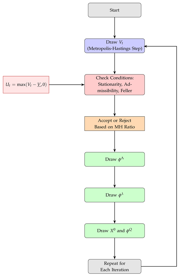
Appendix B. Workflow Diagram: Yield Curve Modeling and Inference
Appendix C. Algorithm: Yield Curve Inference via PCA, Kalman and MCMC
| Algorithm 1:MCMC Algorithm with Kalman Filtering for State-Space Models |
|
References
- Duffee, G.R. Term premia and interest rate forecasts in affine models. The Journal of Finance 2002, 57, 405–443. [Google Scholar] [CrossRef]
- Collin-Dufresne, P.; Goldstein, R.S. Do bonds span the fixed income markets? Theory and evidence for unspanned stochastic volatility. The Journal of Finance 2002, 57, 1685–1730. [Google Scholar] [CrossRef]
- Collin-Dufresne, P.; Goldstein, R.S.; Jones, C.S. Identification of maximal affine term structure models. The Journal of Finance 2008, 63, 743–795. [Google Scholar] [CrossRef]
- Piazzesi, M. Affine term structure models. In Handbook of financial econometrics: Tools and Techniques; Elsevier, 2010; pp. 691–766.
- Riva, R. How much unspanned volatility can different shocks explain? Available at SSRN 4878175 2024.
- Bikbov, R.; Chernov, M. Term structure and volatility: Lessons from the Eurodollar markets. Available at SSRN 562454 2004.
- Collin-Dufresne, P.; Goldstein, R.S.; Jones, C.S. Can interest rate volatility be extracted from the cross section of bond yields? Journal of Financial Economics 2009, 94, 47–66. [Google Scholar] [CrossRef]
- Dai, Q.; Singleton, K.J. Specification analysis of affine term structure models. The Journal of Finance 2000, 55, 1943–1978. [Google Scholar] [CrossRef]
- Diebold, F.X.; Mariano, R.S. Comparing predictive accuracy. Journal of Business & economic statistics 2002, 20, 134–144. [Google Scholar]
- Hansen, J.W. Unspanned stochastic volatility in the linear-rational square-root model: Evidence from the Treasury market. Journal of Banking & Finance 2025, 171, 107354. [Google Scholar]
- Andreasen, M.M.; Jørgensen, K.; Meldrum, A. Bond risk premiums at the zero lower bound. Journal of Econometrics 2025, 247, 105939. [Google Scholar] [CrossRef]
- Andersen, T.G.; Benzoni, L. Do bonds span volatility risk in the US Treasury market? A specification test for affine term structure models. The Journal of Finance 2010, 65, 603–653. [Google Scholar] [CrossRef]
- Collin-Dufresne, P.; Jones, C.; Goldstein, R. Can interest rate volatility be extracted from the cross section of bond yields? An investigation of unspanned stochastic volatility 2004. [Google Scholar] [CrossRef]
- Heidari, M.; Wu, L. Term structure of interest rates, yield curve residuals, and the consistent pricing of interest rate derivatives. Yield Curve Residuals, and the Consistent Pricing of Interest Rate Derivatives (September 10, 2002) 2002.
- Ang, A.; Piazzesi, M.; Wei, M. What does the yield curve tell us about GDP growth? Journal of Econometrics 2006, 131, 359–403. [Google Scholar] [CrossRef]
- Cheridito, P.; Filipović, D.; Kimmel, R.L. Market price of risk specifications for affine models: Theory and evidence. Journal of Financial Economics 2007, 83, 123–170. [Google Scholar] [CrossRef]
- Duffie, D.; Kan, R. A yield-factor model of interest rates. Mathematical finance 1996, 6, 379–406. [Google Scholar] [CrossRef]
- Singleton, K.J. Empirical dynamic asset pricing: model specification and econometric assessment; Princeton University Press, 2006.
- López-Pérez, A.; Febrero-Bande, M.; González-Manteiga, W. Estimation and specification test for diffusion models with stochastic volatility. Statistical Papers 2025, 66, 40. [Google Scholar] [CrossRef]
- Aït-Sahalia, Y.; Li, C.; Li, C.X. Maximum likelihood estimation of latent Markov models using closed-form approximations. Journal of Econometrics 2024, 240, 105008. [Google Scholar] [CrossRef]
- Elerian, O.; Chib, S.; Shephard, N. Likelihood inference for discretely observed nonlinear diffusions. Econometrica 2001, 69, 959–993. [Google Scholar] [CrossRef]
- Stroud, J.R.; Müller, P.; Polson, N.G. Nonlinear state-space models with state-dependent variances. Journal of the American Statistical Association 2003, 98, 377–386. [Google Scholar] [CrossRef]
- Johannes, M.; Polson, N. MCMC methods for continuous-time financial econometrics. In Handbook of financial econometrics: Applications; Elsevier, 2010; pp. 1–72.
- Litterman, R.B.; Scheinkman, J.; Weiss, L. Volatility and the yield curve. The Journal of Fixed Income 1991, 1, 49–53. [Google Scholar] [CrossRef]
- Kumar, R.; Carroll, C.; Hartikainen, A.; Martin, O. ArviZ a unified library for exploratory analysis of Bayesian models in Python. Journal of Open Source Software 2019, 4, 1143. [Google Scholar] [CrossRef]
- Christoffersen, P.; Diebold, F.X. Financial asset returns, market timing, and volatility dynamics. Market Timing, and Volatility Dynamics (January 2, 2002) 2002.
| 1 | [7] decomposes the state variable X into ; where includes all the state variables ,, and , but exclude . The reason is that only affects the factor covariance matrix. They condition on the entire path of, write and in linear Gaussian state space form. The draws involving V can be done using relatively inefficient MH. |
| 2 | Risk-neutral parameters and are not identifiable under USV, hence they are replaced by , and [7]. |
| 3 |
We use the [9] test to assess whether forecast USV significantly outperforms USV in terms of bias and RMSE. The global DM test statistic evaluates the null hypothesis of equal predictive accuracy across the full forecast horizon. Significance is indicated as follows: **p-value , *p-value , p-value .
In addition to the global DM statistic, we compute standardised per-point loss differentials to highlight localized forecast performance differences. Each per-point z-score is defined as:
, where is the pointwise difference in forecast losses, is the mean loss difference, and is the sample standard deviation. Significance levels per point are marked by: ***, **, *
|
Figure 1.
Cumulative explained variance in percentages, is plotted against number of principal components. The green dotted line with dots and blue line represent the cumulative variance for models and fitted yields, respectively. A grey dotted line is the maximum level of 99.97% beyond which the remaing 0.03% represented by a blue line is negligible.
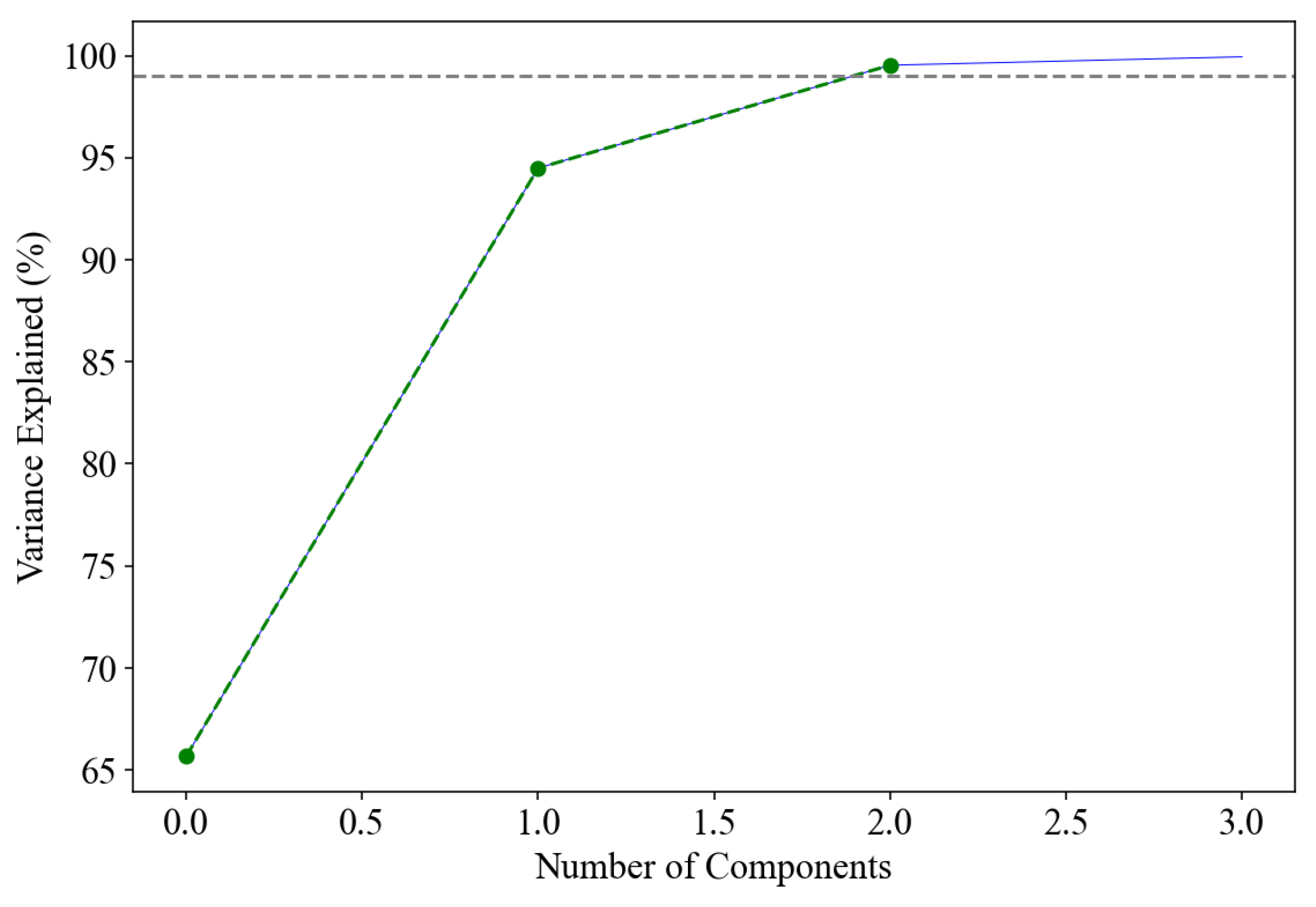
Figure 2.
A sample of posterior parameter histograms for the USV model. These are the risk-neutral drift parameters except for the and . The magenta line represents a theoretical Gaussian density plot. The histograms exhibit a unimodal shape in most cases, which confirm a succesfull convergence and mixing.
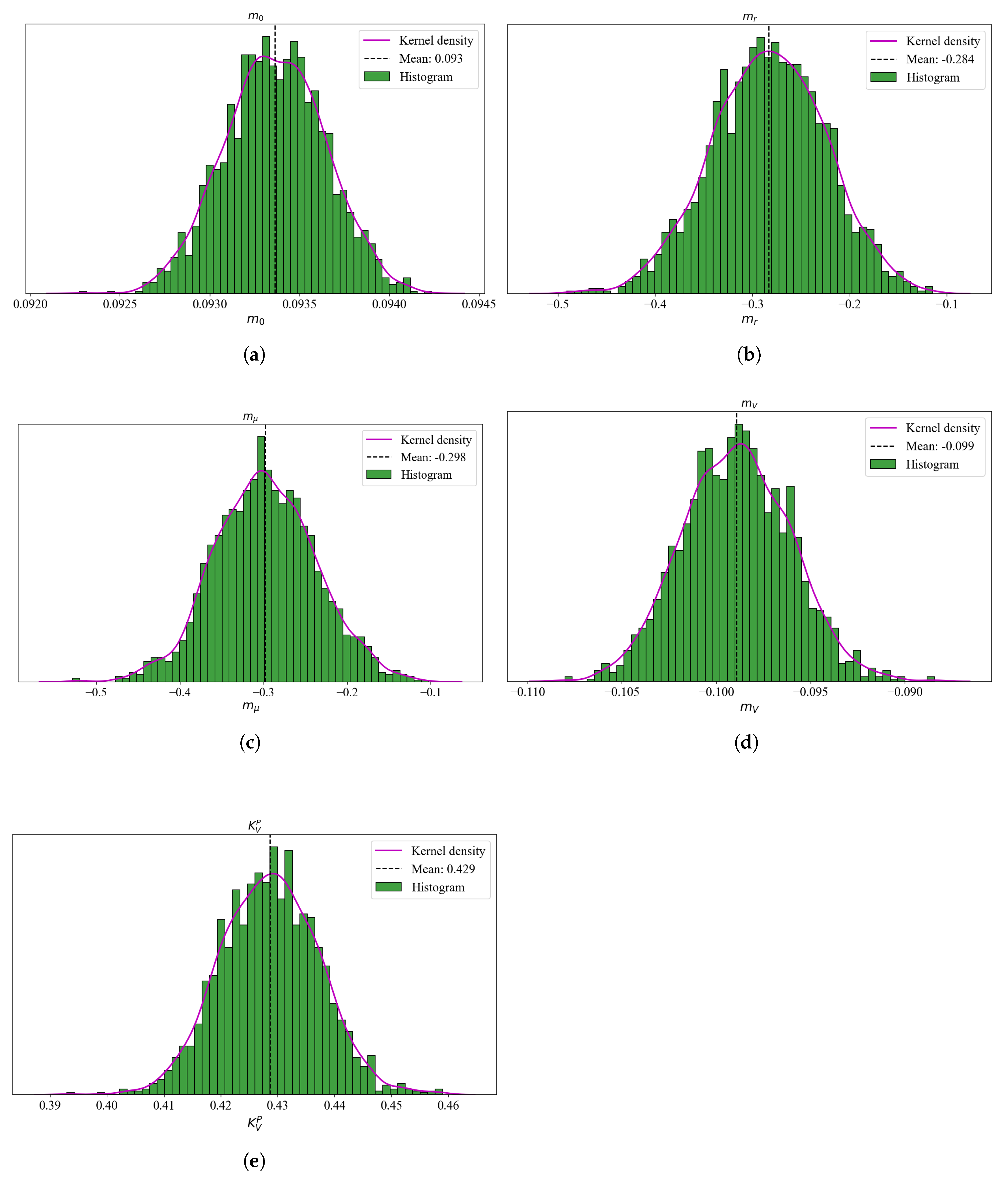
Figure 3.
A sample of posterior parameter histograms for the USV model are plotted. Specifically, these are the risk-neutral drift parameters except for the and . For each histogram, a plot in magenta, represents a theoretical Gaussian density plot. The histograms exhibit a unimodal shape in most cases, which confirm a succesfull convergence and mixing.
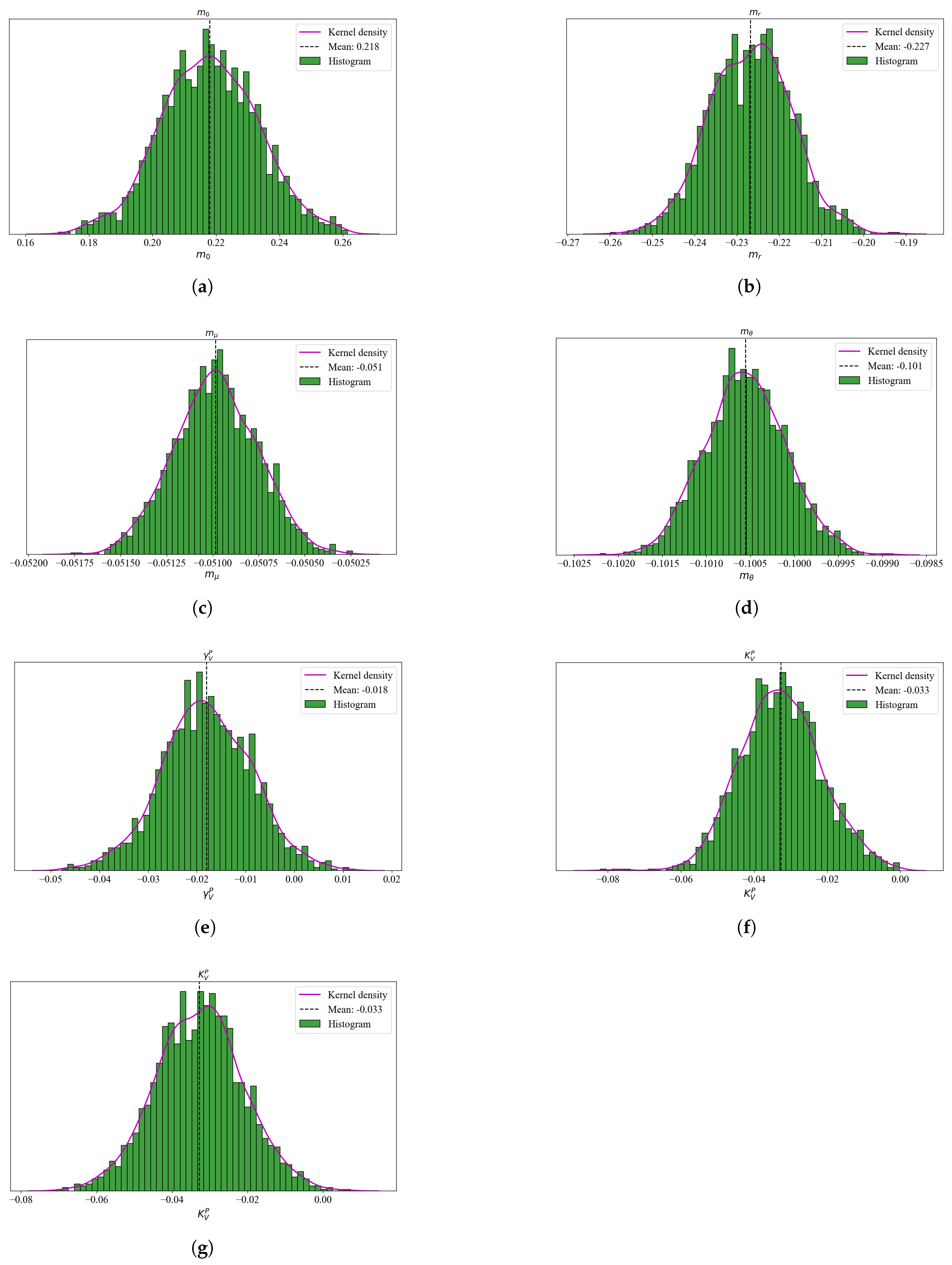
Figure 4.
Conditional and uncoditional volatility are plotted with the probability distributions of parameters. (a) USV model-implied conditional volatilty in blue, plotted with a 26-week rolling volatility in green. (b)USV model-implied unconditional volatilty in blue and shown within the 95% confidence bounds, is plotted with a 26-week rolling volatility in green. (c) USV model-implied conditional volatilty in blue, plotted with a 26-week rolling volatility in green. (d)USV model-implied unconditional volatility in blue and shown within the 95% confidence bounds, is plotted with a 26-week rolling volatility in green. Conditional volatilities are plotted against a time period 2016 - 2024 while the unconditional volatilities are plotted against the maturities.
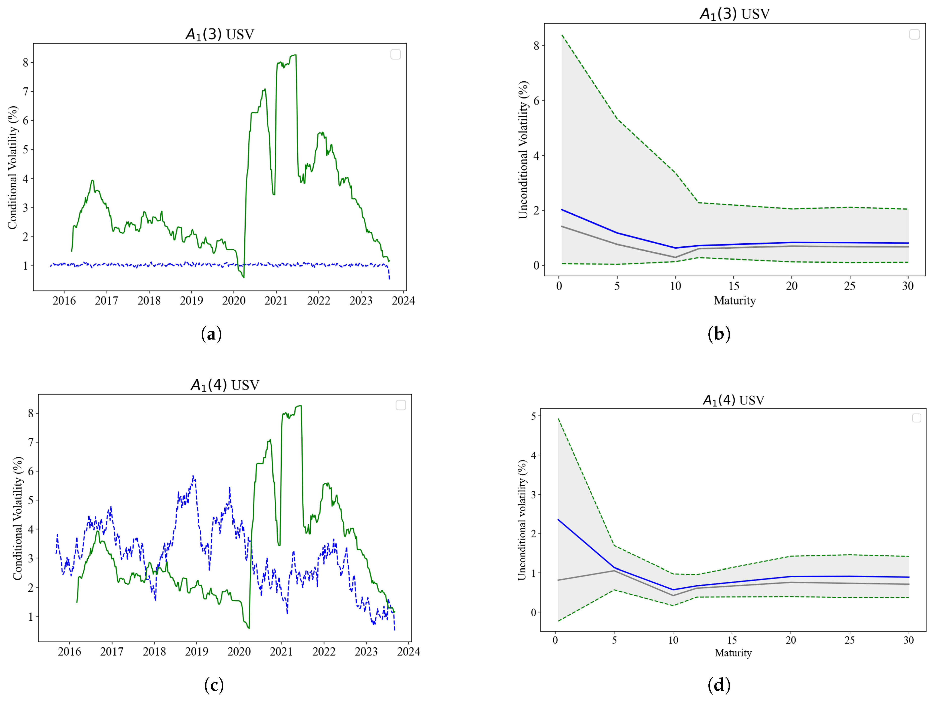
Figure 5.
Market price of risk in basis points is plotted against the time series for the period 2013 - 2024. The first sub-figure (a) plots the model USV and second (b) plots USV both against time. They are based on the propotional relationship between and the essentially affine .
Figure 5.
Market price of risk in basis points is plotted against the time series for the period 2013 - 2024. The first sub-figure (a) plots the model USV and second (b) plots USV both against time. They are based on the propotional relationship between and the essentially affine .
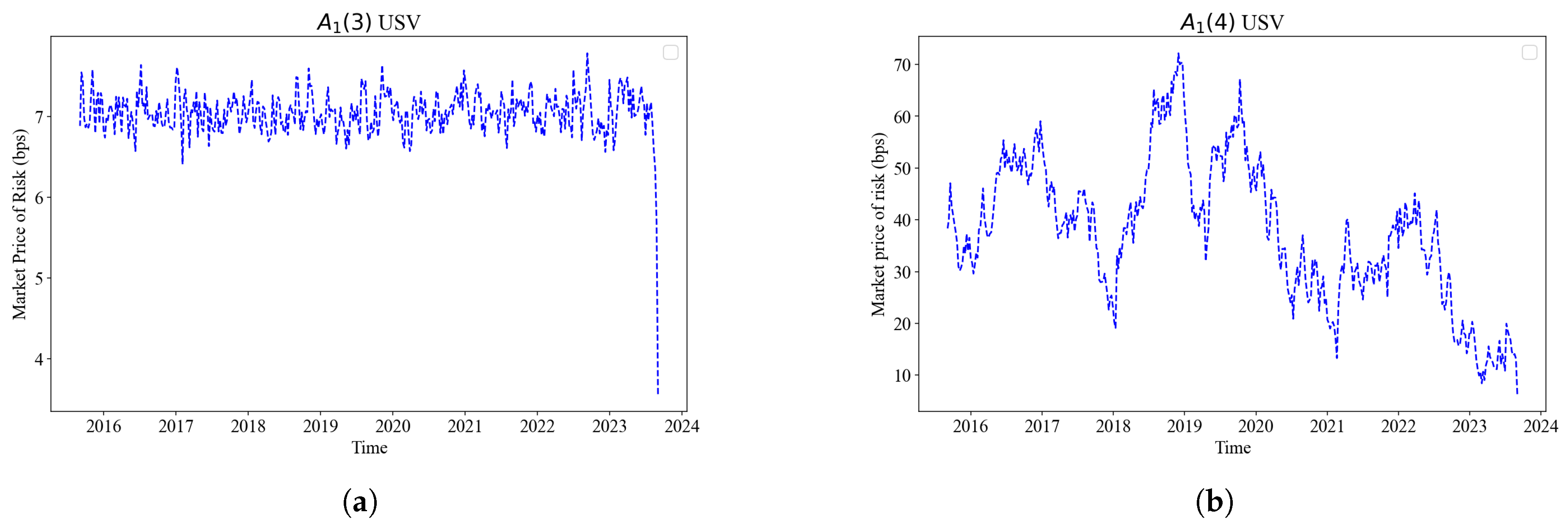

Table 1.
Principal components of the zero coupon yields for the SA government treasury bond over maturities 3 months, 5, 10, 12, 20, 25 and 30 years. The second row from the bottom provides details about explained variances for individual components, which by observation, are declining from 66.06% for the first component, followed by 30.14% for the second one, thereafter dropping to almost zero. The last row represents the cumulative percentages confirming that the first three components contibute more to variation than the remaining others.
| Principal components | |||||||
|---|---|---|---|---|---|---|---|
| 1 | 2 | 3 | 4 | 5 | 6 | 7 | |
| 3 -month | -0.10 | 0.86 | -0.33 | 0.13 | -0.13 | -0.33 | -0.06 |
| 5-year | 0.02 | 0.36 | -0.08 | -0.50 | 0.44 | 0.58 | 0.28 |
| 10-year | 0.17 | -0.03 | 0.04 | -0.37 | -0.51 | -0.25 | 0.71 |
| 1 | 2 | 3 | 4 | 5 | 6 | 7 | |
| 12-year | 0.30 | -0.11 | -0.28 | 0.52 | 0.52 | -0.18 | 0.51 |
| 20-year | 0.60 | 0.00 | -0.37 | 0.21 | -0.43 | 0.50 | -0.15 |
| 25-year | 0.45 | 0.34 | 0.80 | 0.20 | 0.05 | 0.02 | 0.01 |
| 30-year | 0.56 | -0.08 | -0.16 | -0.50 | 0.27 | -0.46 | -0.36 |
| Explained Variance (%) | 66.06 | 30.14 | 3.77 | 0.03 | 0 | 0 | 0 |
| Cumulative Variance (%) | 66.06 | 96.2 | 99.97 | 100 | 100 | 100 | 100 |
Table 2.
Posterior distribution for key risk-neutral drift and covariance parameters for model compared to . The parameters are fitted to the weekly approximated zero yields for the period October 2013 to September 2024. Both models are distinguished from the unrestricted maximal model by restricted parameters. These restricted parameters are shown as undelined and are a function of normal parameters. The table consists of point estimates, based on mean values of the posterior parameter distribution, and confidence interval bounds (in square brackets). Confidence interval bounds for the point estimates are computed as 2.5 and 97.5 percentiles of the posterior distribution.
| Parameter | (3) USV | $A_1(4) USV |
|---|---|---|
| 0.0012 [0.0009, 0.0015] |
0.0010 [0.0010, 0.0010] |
|
|
-0.3588 [-0.4171, -0.3005] |
-0.0780 [-0.1147, -0.0414] |
|
|
-0.8077 [-1.1711, -0.4443] |
-0.0576 [-0.0676, -0.0476] |
|
| -0.1113 [-0.1242, -0.0984] |
||
|
-0.3152 [-1.0949, 0.4645] |
-0.0196 [-0.0203, -0.0189] |
|
| 0.0009 [[0.0009, 0.0009] |
0.0020 [0.0019, 0.0021] |
|
| 0.4457 [0.4414, 0.4500] |
1.0450 [1.0129, 1.0770] |
|
| 0.0071 [-0.0048, 0.0189] |
0.0258 [-0.0230, 0.0746] |
|
| 0.0816 [-0.1823, 0.3454] |
0.0190 [0.0016, 0.0365] |
|
|
0.0101 [0.0098, 0.0104] |
||
| 0.0003 [-0.0007, 0.0013] |
0.0001 [-0.0000, 0.0002] |
|
| 1.0e-06 [1.0e-06, 1.0e-06] |
0.0001 [0.0001, 0.0001] |
|
| -0.4622 [-0.5098, -0.4146] |
-0.3086 [-0.3226, -0.2945] |
|
|
-0.0503 [-0.0524, -0.0482] |
||
|
-0.0507 [-0.0523, -0.0491] |
||
| -0.0507 [-0.0533, -0.0481] |
-0.0973 [-0.1017, -0.0929] |
|
| -0.2237 [-0.2456, -0.2018] |
-0.0951 [-0.0989, -0.0914] |
|
|
0.1043 [0.0992, 0.1094] |
Table 3.
Posterior distribution for key risk-premium parameters for model compared to . The parameters are fitted to the weekly approximated zero yields for the period October 2013 to September 2024. The table consists of point estimates, based on mean values of the posterior parameter distribution, and confidence interval bounds (in square brackets). Confidence interval bounds for the point estimates are computed as 2.5 and 97.5 percentiles of the posterior distribution.
| Parameter | (3) USV | $A_1(4) USV |
|---|---|---|
| -0.0122 [-0.0144, -0.0100] |
-0.0102 [-0.0104, -0.0099] |
|
| -0.0506 [-0.0543, -0.0469] |
-0.0478 [-0.0490, -0.0465] |
|
| -0.0475 [-0.0524, -0.0427] |
-0.0495 [-0.0510, -0.0480] |
|
| -0.0098 [-0.0107, -0.0089] |
-0.0102 [-0.0105, -0.0099] |
|
| 0.0947 [0.0872, 0.1021] |
0.0495 [0.0478, 0.0512] |
|
| 0.2783 [0.2518, 0.3047] |
0.1025 [0.0961, 0.1089] |
|
| 47.4552 [42.8097, 52.1008] |
10.2594 [9.7983, 10.7205] |
|
| -0.0000 [-0.0000, -0.0000] |
-0.0001 [-0.0001, -0.0001] |
|
| 0.0579 [0.0499, 0.0659] |
0.0941 [0.0890, 0.0992] |
|
| -10.5910 [-11.5637, -9.6183] |
-1.9671 [-2.0473, -1.8868] |
|
| 0.0516 [0.0485, 0.0548] |
0.0201 [0.0196, 0.0206] |
|
| 0.0201 [0.0197, 0.0205] |
||
| 0.0193 [0.0183, 0.0203] |
||
| 0.0208 [0.0201, 0.0215] |
||
| 0.0211 [0.0200, 0.0221] |
||
| 0.0193 [0.0181, 0.0204] |
Table 4.
The results of estimation for a sample of drift parameters for the model are presented below. The purpose of the report is to determine the reliability of the posterior parameters.
Table 4.
The results of estimation for a sample of drift parameters for the model are presented below. The purpose of the report is to determine the reliability of the posterior parameters.
| Mean | Std | HDI (2.5%) | HDI (97.5%) | MCSE (Mean) | MCSE (Std) | ESS (bulk) | ESS (tail) | ||
|---|---|---|---|---|---|---|---|---|---|
| 0.001 | 0 | 0.001 | 0.001 | 0 | 0 | 2326 | 1346 | 1 | |
| -0.284 | 0.059 | -0.398 | -0.171 | 0.001 | 0.001 | 2160 | 1106 | 1 | |
| -0.299 | 0.063 | -0.421 | -0.177 | 0.001 | 0.001 | 2555 | 1429 | 1 | |
| -0.099 | 0.003 | -0.105 | -0.093 | 0 | 0 | 2312 | 1495 | 1 | |
| 0.428 | 0.008 | 0.411 | 0.445 | 0 | 0 | 2113 | 1149 | 1 | |
| 0.007 | 0.005 | 0 | 0.016 | 0 | 0 | 975 | 674 | 1 |
Table 5.
The results of estimation for a sample of drift parameters for the model are presented below. The purpose of the report is to determine the reliability of the posterior parameters.
Table 5.
The results of estimation for a sample of drift parameters for the model are presented below. The purpose of the report is to determine the reliability of the posterior parameters.
| Mean | Std | HDI (2.5%) | HDI (97.5%) | MCSE (Mean) | MCSE (Std) | ESS (bulk) | ESS (tail) | ||
|---|---|---|---|---|---|---|---|---|---|
| 0.093 | 0 | 0.093 | 0.094 | 0 | 0 | 3775 | 1808 | 1 | |
| -0.227 | 0.01 | -0.247 | -0.209 | 0 | 0 | 2626 | 1503 | 1 | |
| -0.051 | 0 | -0.051 | -0.051 | 0 | 0 | 2549 | 1383 | 1 | |
| -0.101 | 0 | -0.101 | -0.100 | 0 | 0 | 2241 | 1407 | 1 | |
| -0.200 | 0 | -0.201 | -0.199 | 0 | 0 | 3182 | 1548 | 1 | |
| -0.018 | 0.009 | -0.036 | -0.001 | 0 | 0 | 2589 | 1617 | 1 | |
| -0.032 | 0.011 | -0.052 | -0.010 | 0 | 0 | 2162 | 1650 | 1 |
Table 6.
In-sample and out-sample zero yields are compared to model-fitted estimates for the 0.25, 5,10, 12, 20, 25, and 30-year maturities. The fifth column reflects the statistical significance at 5% and 1%, labelled with ** and *, respectively. Bias is determined in terms of the null hypothesis that bias is zero, while RMSE is based on a pairwise analysis of the models. Inequality sign provides the direction of a loss.
| Maturity | USV | Loss direction | USV | Significance |
|---|---|---|---|---|
| In-sample RMSE1 | ||||
| 0.25 | 0.0703 | < | 0.0683 | * |
| 5 | 0.0868 | < | 0.0856 | |
| 10 | 0.0958 | < | 0.0946 | |
| 12 | 0.0994 | < | 0.0984 | |
| 20 | 0.1045 | < | 0.1040 | |
| 25 | 0.1053 | < | 0.1043 | |
| 30 | 0.1046 | < | 0.1040 | |
| In-sample bias 2 | ||||
| 0.25 | 0.0660 | 0.0661 | ||
| 5 | 0.0841 | 0.0842 | ||
| 10 | 0.0938 | 0.0939 | ||
| 12 | 0.0978 | 0.0979 | ||
| 20 | 0.1035 | 0.1036 | ||
| 25 | 0.1039 | 0.1041 | ** | |
| 30 | 0.1035 | 0.1036 | ||
| Out-sample RMSE3 | ||||
| 0.25 | 15.3984 | < | 0.086407 | ** |
| 5 | 0.2219 | < | 0.0896 | |
| 10 | 0.0780 | > | 0.1012 | |
| 12 | 0.0612 | > | 0.1095 | |
| 20 | 0.0389 | > | 0.1233 | |
| 25 | 0.0505 | > | 0.1241 | |
| 30 | 0.0256 | > | 0.1232 | |
| Out-sample bias4 | ||||
| 0.25 | -12.0832 | 0.0848 | ** | |
| 5 | 0.0855 | 0.0879 | ||
| 10 | 0.0078 | 0.0996 | ||
| 12 | -0.0549 | 0.1079 | ||
| 20 | -0.0369 | 0.1218 | ||
| 25 | -0.0495 | 0.1227 | ||
| 30 | -0.0201 | 0.1218 | ||
1 DM t-statistic = 6.1233, p-value = 0.0009*** → Reject . Better model: USV (based on lower RMSE). 2DM t-statistic = -8.0000, p-value = 0.0002***→ Reject . Better model: USV is significantly less biased. 3DM t-statistic = 0.9999, p-value = 0.3559 → Fail to reject . Better model: USV (based on lower RMSE). . 4DM t-statistic = 0.9571, p-value = 0.3755 → Fail to reject . Better model: USV (based on lower bias).
Table 7.
Model-implied volatility proxy for the weekly yield returns computed as a 26-weeks rolling standard deviation. Initially, the rolling statistic is computed for the 3-month (short-end) yields, then compared to the 12-year (mid-term) and 30-year (long-end). The model-implied volatility is derived as filtered from each model. Other time series variables for the same maturities are the GARCH, brent crude, USDZAR, and the three PCA factors level, slope, and curvature. The speaman correlation is calculated between the model-implied volatility and these variables.
| Maturities | 0.25 | 12 | 30 | 0.25 | 12 | 30 |
| Actual vs Model Average Yield | 0.964 | 0.964 | 0.964 | 1.000 | 1.000 | 1.000 |
| Actual vs Model Sope | 0.974 | 0.974 | 0.974 | 0.919 | 0.933 | 0.933 |
| Actual vs Model Curvature | 0.989 | 0.989 | 0.989 | 0.733 | 0.749 | 0.749 |
| Rolling vs Model Volatility | 0.054 | 0.002 | -0.037 | 0.550 | 0.157 | -0.049 |
| SA Rand Dollar vs Model Volatility | 0.007 | -0.024 | 0.058 | 0.408 | 0.122 | 0.613 |
| Brent Crude vs Model Volatility | 0.050 | 0.064 | 0.000 | 0.216 | 0.055 | 0.478 |
| GARCH vs Model Volatility | 0.026 | -0.040 | -0.055 | 0.128 | 0.145 | -0.019 |
| Curvature vs Model Volatility | -0.119 | 0.034 | -0.034 | -0.421 | -0.049 | -0.297 |
| Curvature vs Model Variance | -0.119 | 0.034 | -0.034 | -0.421 | -0.049 | -0.297 |
Table 8.
In-Sample and Out-Sample one-week forecast of two different volatility proxies and for the 0.25, 5,10, 12, 20, 25, and 30-year maturities. The fifth column reflects the statistical significance at 5% and 1%, labelled with ** and *, respectively. Bias is determined in terms of the null hypothesis that bias is zero, while RMSE is based on a pairwise analysis of the models. Inequality sign provides the direction of a loss.
| Maturity | USV | Loss Direction | USV | Significance |
|---|---|---|---|---|
| In-Sample RMSE of weekly (bps)5 | ||||
| 0.25 | 131.83 | < | 37.53 | ** |
| 5 | 50.38 | < | 25.22 | |
| 10 | 39.66 | < | 20.54 | |
| 12 | 31.97 | > | 45.51 | |
| 20 | 27.15 | > | 79.48 | |
| 25 | 27.50 | > | 81.28 | |
| 30 | 26.69 | > | 78.63 | |
| In-Sample RMSE of (bps) 6 | ||||
| 0.25 | 44.68 | < | 39.64 | ** |
| 5 | 28.42 | < | 25.92 | |
| 10 | 26.91 | < | 25.22 | |
| 12 | 26.92 | < | 24.97 | |
| 20 | 27.75 | < | 24.72 | |
| 25 | 26.85 | < | 23.90 | |
| 30 | 27.10 | < | 24.26 | |
| Out-Sample RMSE of weekly (bps)7 | ||||
| 0.25 | 18.35 | < | 14.87 | |
| 5 | 33.54 | < | 33.22 | |
| 10 | 41.45 | < | 41.39 | |
| 12 | 45.38 | < | 44.91 | |
| 20 | 56.44 | < | 49.60 | |
| 25 | 57.51 | < | 50.00 | |
| 30 | 58.16 | < | 50.18 | |
| Out-Sample RMSE of (bps)8 | ||||
| 0.25 | 15.60 | < | 14.41 | |
| 5 | 29.58 | < | 28.56 | |
| 10 | 38.52 | < | 37.26 | |
| 12 | 41.57 | < | 40.24 | |
| 20 | 39.71 | < | 38.18 | |
| 25 | 40.57 | < | 38.88 | |
| 30 | 40.56 | < | 38.82 | |
5 DM t-statistic = 0.0527, p-value = 0.9597 → Fail to reject . Better model: USV (based on lower RMSE). 6DM t-statistic = 2.4035, p-value = 0.0530* → Fail to reject . Better model: USV (based on lower RMSE). 7DM t-statistic = 6.7912, p-value = 0.0005*** → Reject . Better model: USV (based on lower RMSE). 8 DM t-statistic = 6.7912, p-value = 0.0005*** → Reject . Better model: USV (based on lower RMSE).
Table 9.
Regressions for weekly realised volatilities 3-month and 30-year maturities. These regressions are performed on different variables. They are reflected as systematic risks according to coefficients for each variable and standard errors in square brackets. For each models there are two rows; first without PCA factors and the scond with PCA factors level, slope and curvature. These regressions were performed on the time series variables for the period 2013 to 2024. Top panel are the regression results for the 3-month weekly realised volatility and the bottom panel is for the 30-year weekly realised volatilty.
| Variable | Intercept() | Volatility() | Level | Slope | Curvature | |
|---|---|---|---|---|---|---|
| 3-Month Yield Volatilities | ||||||
| GARCH(1,1) | 0.202 [0.015] | 0.395 [0.036] | 0.240 | |||
| 0.210 [0.013] | 0.228 [0.036] | 0.477 | -0.025 [0.005] | -0.112 [0.009] | -0.279*** [0.025] | |
| USV | 1.196 [0.2619] | -8.473 [2.576] | 0.027 | |||
| 0.977 [0.203] | -6.876 [1.999] | 0.428 | -0.027 [0.005] | -0.132 [0.009] | -0.334 [0.024] | |
| USV | 0.069 [0.090] | 0.810 [0.274] | 0.022 | |||
| 0.696 [0.126] | -1.321 [0.3956] | 0.427 | -0.043 [0.007] | -0.173 [0.016] | -0.364 [0.025] | |
| 30-Year Yield Volatilities | ||||||
| GARCH(1,1) | 0.068 [0.007] | 0.472 [0.045] | 0.221 | |||
| 0.067 [0.007] | 0.447 [0.045] | 0.241 | -0.005 [0.002] | -0.005 [0.004] | -0.023 [0.009] | |
| USV | 0.350 [0.085] | -2.144 [0.835] | 0.017 | |||
| 0.317 [0.084] | -1.862 [0.8262] | 0.062 | -0.007 [0.002] | -0.006 [0.004] | -0.032 [0.010] | |
| USV | 0.038 [0.025] | 0.302 [0.080] | 0.035 | |||
| -0.293 [0.046] | 1.393 [0.150] | 0.221 | 0.010 [0.003] | 0.037 [0.006] | -0.032 [0.009] | |
Disclaimer/Publisher’s Note: The statements, opinions and data contained in all publications are solely those of the individual author(s) and contributor(s) and not of MDPI and/or the editor(s). MDPI and/or the editor(s) disclaim responsibility for any injury to people or property resulting from any ideas, methods, instructions or products referred to in the content. |
© 2025 by the authors. Licensee MDPI, Basel, Switzerland. This article is an open access article distributed under the terms and conditions of the Creative Commons Attribution (CC BY) license (http://creativecommons.org/licenses/by/4.0/).
Copyright: This open access article is published under a Creative Commons CC BY 4.0 license, which permit the free download, distribution, and reuse, provided that the author and preprint are cited in any reuse.


