Submitted:
09 June 2025
Posted:
10 June 2025
You are already at the latest version
Abstract
In this paper, we study a geometric framework for a class of second order differential systems arising in classical and relativistic mechanics. For this class of systems, we derive the necessary and sufficient conditions for their Lagrangian description. Using the discrete variational principle, we present a class of variational integrators by splitting the Lagrangian. We then prove that the newly derived numerical methods are equivalent to composition methods. When applied to the Kepler problem, these methods show superior performance over classical methods. By establishing the theory of modified equations and modified Lagrangians, we provide error estimates for the new variational methods. The analysis of the Laplace--Runge--Lenz (LRL) vector confirms the numerical performance.
Keywords:
inverse variational problem
; Kepler problem
; Modified Lagrangian
; Noether’s theorem
; variational integrator
1. Introduction
Some important physical problems, ranging from celestial mechanics to magnetized plasmas, naturally exhibit rich conservative invariants. These problems are often connected to geometric structures, which have garnered increasing interest in recent studies [1,2,3]. Examples of such structures include Hamiltonian, volume-preserving, Poisson, contact, and integral-preserving systems. Among these, variational structures play a central role in modeling systems in various applications. The inverse variational principle [4] provides the foundational approach for studying systems within the Lagrangian framework [4,5,6]. Through Legendre transformations, the Hamiltonian and Lagrangian formulations are shown to be equivalent. In the variational framework, variational integrators are constructed by discretizing the Lagrangian. Numerical methods are then derived via the discrete Euler–Lagrange equations. Further details can be found in [7] and the references therein. These numerical methods consistently demonstrate superior efficiency and stability. Such methods have been successfully applied to simulate various physical problems, including soliton wave equations [8,9], charged particle dynamics in electromagnetic fields [10,11,12,13], and kinetic models in plasma physics [14,15], among others.
In the theory of backward error analysis (or modified equations theory), a numerical method is interpreted as the exact solution of a nearby “modified” system. According to this theory, structure-preserving numerical methods satisfy modified equations that retain the same structure as the original system. This explains the superior behavior of structure-preserving numerical methods in long-term simulations [16,17,18]. In [19], the concept of modified equations has been extended to variational equations. This theory can be extended to analyze adaptive time-step variational integrators [20] and Hamiltonian partial differential equations (PDEs) [21,22], broadening its applicability to a wider range of systems.
This paper focuses on second order ordinary differential systems. We establish the necessary and sufficient conditions for variational formulations of a class of systems. This framework naturally encompasses classical and relativistic dynamics, as well as the motion of charged particles under Lorentz forces. In this variational framework, variational integrators are constructed by discretizing the Lagrangian. To enhance computational efficiency, we introduce new variational integrators by splitting the Lagrangian. Through Legendre transformations, we prove that these methods are equivalent to composition methods. We use the Kepler problem as an example, where geometric integrators have been shown to perform well in long-term numerical simulations [23,24,25,26]. The Kepler system, a super-integrable system that models gravitational motion, involves conserved quantities such as energy, angular momentum, and the Laplace–Runge–Lenz (LRL) vector [27]. We investigate the superior numerical performance of variational integrators in simulating the Kepler problem. In addition to energy and momentum, the LRL vector, a hidden conserved quantity [28], governs orbital geometry. By Noether’s Theorem [29], we show the variational symmetries for energy, momentum, and the LRL vector. Through the development of modified equations and modified Lagrangians, we understand the solution of variational integrators as exact solutions of the perturbed Kepler system. Using modified equation theory, we demonstrate that the modified Kepler equation remains integrable, ensuring bounded errors in preserving energy and momentum. However, the modified equation loses super-integrability, leading to a quasi-periodic orbit instead of a periodic one. We explicitly derive the modified Lagrangians for the symplectic Euler, Störmer—Verlet methods, and the newly derived variational integrators. Perturbation theory reveals the super-convergence of these new variational integrators in preserving the LRL vector.
The paper is organized as follows. Section 2 establishes the necessary and sufficient conditions for describing second order systems within a variational framework. Section 3 constructs variational discretizations by splitting the Lagrangian. The resulting numerical discretization is shown to be equivalent to the composition method. Using classical and relativistic Kepler systems as examples, we illustrate the numerical methods and present variational symmetries for energy, momentum, and the LRL vector. Section 4 develops the theory of modified equations and modified Lagrangians. The recursive expressions for the Nyström methods is provided. For the Kepler problem, we also analyze the errors of the newly proposed variational integrators in conserving quantities. In Section 5, we apply the newly derived variational integrators to solve the Kepler problem. The numerical results demonstrate the superior performance of these methods. We further analyze the numerical performance using the modified Lagrangian theory. Additionally, we apply the variational integrators to solve the relativistic Kepler system. Finally, Section 6 concludes the paper.
2. Variational Principle in Lagrangian Formalism
We begin this section by introducing the inverse variational methods presented in [4,5,6]. Let be a real Hilbert space with inner product . Let be an operator. The operator N is called as symmetric if , where is the adjonit operator defined by for . The Fréchet derivative of N at , denoted , is the linear operator satisfying
According to the Vainberg’s Theorem in [4], we have
Theorem 1.
Let N be a operator defined on . If the Fréchet derivative of N is symmetric, i.e. , then there exists a functional S on , constructed as
such that , where the variational derivative is defined by , .
In this paper, we mainly focus on the variational description for the system of second order differential equations. Consider the systems governed by
where is an symmetric matrix.
Theorem 2.
System (2.1) admits a variational formulation if and only if
hold for all .
Proof.
Define . The variational calculus gives
The adjoint of is defined as
From the integration by parts, we have
Therefore,
According to Theorem 1, The system is variational if and only if (2.3) and (2.4) are identical. Comparing (2.3) and (2.4) leads to
The above equality holds for arbitrary , thus the coefficients in terms , and vanish. Since M is symmetric, this implies exactly that
This completes the proof of the theorem. □
Assuming and f is linear in , we can rewrite the above theorem as follows.
Theorem 3.
For and , system (2.1) is variational if and only if
where .
Proof.
Since M depends only on , (2.2b) simplifies to (2.5a). The condition (2.2c) reduces to
In the above equality, the term on the right-hand side does not depend on , so the coefficients of vanish. □
Remark 1.
Define a differential two-form by . If (2.5a) and (2.5b) hold, then . By Poincaré’s lemma, there exists a one-form such that . This implies . Condition (2.5c) means that φ can be generated from a potential ϕ by .
In more classical applications, M is typically a constant matrix. In this case, for the system to be variational, we only need the conditions for the vector field f.
Theorem 4.
For constant symmetric M, system (2.1) is variational iff
holds for .
Many important physical problem including some relativistic models can have the forms of Theorem 3. Consider the relativistic dynamics (such as a charged particle in a Coulomb potential)
where is the Lorentz factor, c is the speed of light. In the non-relativistic limit (), this reduces to Newtonian mechanics . It is evident that the velocity-dependent terms satisfy the symmetry conditions (2.2a) and (2.5c). This system admits the variational formulation with Lagrangian .
It is well known that from Lagrangian framework it is more convenient to investigate the connections between conservation laws and symmetry properties of dynamical systems based on Noether theorem. The foundational framework requires introducing generalized vector fields and their action on variational principles [6].
A generalized vector field is given by
where contain x and all the derivatives of x and denote its characteristic. The infinite prolongation of is defined as
where denotes j-th order time derivatives.
Definition 1.
A generalized vector field is called a variational symmetry for the functional if there exists a function such that
Given a differential system , if there exists satisfying
then Q is called the characteristic of the nontrivial conservation law .
Theorem 5
(Noether’s theorem). A generalized vector field is a variational symmetry if and only if its characteristic Q is also the characteristic of a conservation law along the solution of Euler–Lagrange equations.
When the system is perturbed, the following proposition holds.
Proposition 1.
Given a Lagrangian L, let and P denote its variational symmetry and the corresponding conserved quantity, respectively. Under the perturbed Lagrangian , P along solutions of satisfies
where is the the Euler operator.
Proof.
By Theorem 5, it gives . For the solution of the perturbed system , we have
Substitution yields . □
3. Discrete Lagrangian Mechanics
Variational integrators preserve geometric structures by discretizing Hamilton’s principle. For foundational theory, see [7]. Consider a uniform time grid with coordinates . The discrete Hamilton’s principle is to find the trajectories extremizing the discrete action functional
Here, is the discretization of L, given by . Its adjoint, denoted by , is defined as . The discrete solution satisfies the discrete Euler—Lagrange equations
Consider the system
with Lagrangian . We discretize the Lagrangian to obtain the variational integrators. By splitting the potential as , we present the following discrete Lagrangian. A first order variational integrator uses the discrete Lagrangian
where , is the N-dimensional vector with the j-th element being 1.
Theorem 6.
The discrete Lagrangian is of order 1. Moreover, the discrete Euler–Lagrange equations for (3.3) generate
It coincides with the composition method
where represents the subsystem, and is the corresponding numerical discretization, given by
Proof.
Using the Taylor expansion at an arbitrary , we have
Substituting these into (3.3), it is easy to known that the discrete Lagrangian has first order accuracy.
Introduce the discrete Legendre transformation
the discrete Euler–Lagrange equation gives
From (3.4) and (3.5), we can derive
This is exactly the composition method . □
The discrete Lagrangian of higher order variational integrators can be constructed by combining and its adjoint
By the discrete Euler–Lagrange equation, these provide the higher order variational integrators.
Theorem 7.
The variational integrators from (3.7) and (3.8) are equivalent to and , respectively.
Proof.
The corresponding discrete Euler–Lagrange equation for (3.7) gives
Introduce the discrete Legendre transformation,
From (3.9b), we know
Combine (3.10) and (3.11), we can prove that . □
As follows, we take the Kepler problem as example to illustrate the new derived variational methods of first and second order.
Kepler problem. The Kepler problem describes the motion of two bodies attracting each other. We focus on the 2-dimensional Kepler problem in the following text. If one body is placed at the origin, and x represents the position of the other body, their dynamics are governed by the following system
where . It is obvious that the Kepler problem (3.12) satisfies Theorem 4, and its Lagrangian is given by
The Kepler problem (3.12) has three conserved quantities: energy, angular momentum, and the Laplace–Runge–Lenz (LRL) vector. When the initial energy , the solution orbit of the Kepler problem is elliptic, such as the motion of one astronomical body moving around another. In this case, the LRL vector determines the orientation and shape of the elliptical orbit. The magnitude equals the orbital eccentricity e, and the vector points along the major axis of the orbit.
Proposition 2.
For the 2D Kepler system (3.12), the following quantities are conserved
- Energy ,
- Angular Momentum ,
- LRL Vector .
Introducing the polar coordinates , the Kepler’s Three Laws [28] are exhibited.
Proposition 3
(Kepler’s Three Laws). For bound orbits (negative energy) in the 2D Kepler problem, we have
- The inverse of the radial distance is given by ;
- The period of the orbit is ;
- The areal velocity is conserved, i.e., .
where a and b represent the semi-major and semi-minor axes of the orbit, is the eccentricity.
Based on Noether’s theorem, for the two-dimensional Kepler problem (3.12), we derive the variational symmetries corresponding to the three conservative quantities expressed in Proposition 2.
Proposition 4.
The variational symmetries associated with the energy, angular momentum, and the LRL vector are as follows:
- ,
- ,
- , .
Proof.
Taking gives the following equality for energy conservation
Suppose the generalized vector field . By Theorem 5, is exactly the variational symmetry of the energy. The other variational symmetries follow analogously from their conservation laws. □
Splitting as , we construct the first order and second order discrete Lagrangians. The first order Lagrangian (3.3) yields the variational integrator through the discrete Euler–Lagrange equations
The second order Lagrangians (3.8) generates the numerical methods
Relativistic Kepler Problems. Considering the relativistic Kepler systems in (2.7) with the potential . By the proper time and relativistic momentum , we reformulate system (2.7) as
where . Let and , where ’·’ denotes differentiation with respect to . By Theorem 4, we learn that the system (3.16) admits a variational formulation with Lagrangian
where and . The system (3.16) has two Hamiltonian formulations. Defining , the system (3.16) admits the standard Hamiltonian form
where and the Hamiltonian is non-separable. Introducing transforms the system into a K-symplectic [1,3] formulation:
where with . In the formulation (3.18), the Hamiltonian becomes separable
By decomposing this Hamiltonian into parts, we derive the K-symplectic subsystems.
The subsystem has the exact solution, which is
For , , the solution of i-th subsystem is
We obtain the K-symplectic method by composing the exact solution of the subsystem.
Theorem 8.
The discrete Lagrangian for (3.16)
generates the variational integrator
This is equivalent to the K-symplectic method (3.19).
Proof.
Introducing the following transformations
with , yields
Reformulating (3.21) leads to
which are exactly the K-symplectic methods (3.19). □
4. Modified Equations for Variational Integrator
We begin this section by introducing the concept of modified equations presented in [19] for second order systems
Definition 2.
For system (4.1), denote the method by . Its modified equation is a formal second order differential equation
satisfying for all n.
Expanding the difference equation around gives
Introducing , it follows from (4.2) that
Taking the derivative of the above equality with respect to t gives
Substituting the higher derivatives into the terms in (4.3), we obtain the following theorem by comparing the coefficients of h on both sides of (4.3).
Theorem 9.
The coefficients in the modified equations (4.2) are uniquely determined recursively by f, , …, , , …, , and their derivatives.
Theorem 9 provides a recursive relation for calculating the coefficients of modified equations. We illustrate this by applying the Nyström methods [2] to (4.1), which results in
Theorem 10.
For the Nyström methods (4.5), the coefficients of modified equation can be achieved by
where is an elementary differential, as described in [2].
Proof.
Using (4.5a) and (4.5b) to eliminate the intermediate variable v yields the scheme
From (4.5a) and (4.5c), we derive
Expanding the left-hand side of (4.6) about gives
Similarly, and on the right term can be expanded about up to , as
Substituting (4.8) and the higher derivatives (4.4) into the right-hand side of (4.6) and comparing the coefficients of the term yields recursive formulas.
thus completing the proof. □
Remark 2.
Generally, the system of modified equations represents a formal divergent series. However, for linear second order systems, we are able to obtain a convergent modified series. Further details can be found in Appendix A.
It is well-known that the system (3.2) has a variational description. However, not all numerical discretizations of this system are variational. A method is variational if and only if its modified equation (4.2) maintains variational structure. By Theorem 4, this requires the coefficients to satisfy
This implies the existence of formal Lagrangian which is called as the modified Lagrangian denoted by .
Definition 3.
The modified Lagrangian is a formal series
whose Euler–Lagrange equations
have the solution matching the variational integrator .
An alternative definition of modified Lagrangian can be found in [19], that is
where . Differentiating (4.10) w.r.t to yields
where boundary terms vanish.
Expand the discrete Lagrangian at , it reads
where x denote , contains x and its derivatives. By Lemma 1 in [19], the discrete action functional over the interval can be expressed as
where are Bernoulli numbers with , and . From (4.10), it follows that
Solving implicitly from the modified Euler–Lagrange equation (4.9) and substituting it into (4.12), we can eliminate and its higher order derivatives in the right-hand side of (4.12). According to Proposition 6 in [19], the term only depends on x and its j order derivatives . Comparing the coefficients of the term on both sides of (4.12), we obtain
Recursively, we can derive the modified Lagrangian as a formal series corresponding to the time step h.
For the system (3.2), the Störmer–Verlet method originates from the discrete Lagrangian
As presented in [19], its second order modified Lagrangian
yields the following modified Euler–Lagrange equation
The symplectic Euler method corresponds to the first order discrete Lagrangian
The discrete Lagrangians (4.13) and (4.16) are weak equivalence [7] as their corresponding variational integrators are the same as
Theorem 11.
For the discrete Lagrangian (4.16), its third order modified Lagrangian is
with corresponding Euler–Lagrange equation
Proof.
Expanding (4.16) around , we obtain
Applying the modified Lagrangian construction (4.12)
It is evident that
which implies that the terms in vanish. Substituting into (4.18) yields (4.17). The Euler–Lagrange equation follows from
□
We illustrate the solutions of truncated modified equations using the pendulum problem. For this, let in (4.1). The modified Lagrangian gives the corresponding modified Hamiltonian via the Legendre transformation. Denote the k-th order truncated Lagrangian by and the corresponding Hamiltonian by . For , the modified Hamiltonian corresponding to is given by
which matches the result in [2]. In Figure 1, we show the numerical solution using the symplectic Euler method from (4.16), along with the exact flow of the pendulum problem, represented by the contour plot of the Hamiltonian. The contour plot of (4.20) shows the exact flow of the modified pendulum problem at first order. The initial conditions are . In Figure 1, the solid line represents the exact solution of the pendulum, while the dotted lines correspond to the symplectic Euler method and the exact solution of the modified pendulum. The results show that the modified pendulum problem provides better agreement between the numerical solution and the exact solution. As we include more terms in the truncation, we expect further improvement. However, since the modified equations are not convergent, there is an optimal truncation level based on asymptotic expansion theory.
For the newly presented variational integrators from (3.3) and (3.8), the modified Lagrangians are established in the following theorem.
Theorem 12.
For the first order discrete Lagrangian (3.3), its modified Lagrangian truncated to order 2 can be formulated as
The corresponding Euler–Lagrange equation takes the following form:
For the second order discrete Lagrangian (3.8), the second truncation of the modified Lagrangian is given by
The corresponding Euler–Lagrange equation can be expressed as
where
Proof.
Without loss of generality, we compute the modified Lagrangian of second truncation for the discrete Lagrangian (3.8). Expand (3.8) about , we derive
Substitute into (4.12), we obtain
We apply to eliminate term in (4.25), this leads to (4.23). With the modified Lagrangian (4.23), the direct calculation provides the modified equation (4.24). □
As discussed earlier, the variational integrator can be interpreted as the exact solution to the modified equations. Consequently, the conservative properties of numerical methods are linked to their modified Lagrangian. Through backward error analysis [2], it is expected that variational integrators can preserve energy and angular momentum over long-time integration. For the Kepler problem, known as super-integrable, we present the following theorem to characterize the preservation of the LRL vector.
Theorem 13.
For the perturbed Kepler problem, let its Lagrangian be . Assume the initial orbits are aligned with the -axis to , then the variation of the LRL vector over one period satisfies
and the change in the angle ω relative to the x-axis is given by
Here, are the LRL characteristics shown in Proposition 4, T is the orbital period, and denotes the T-period average.
Proof.
Under the assumption of the proposition, we have and . According to Proposition 1, it follows that
where and x are the solutions of the perturbed and unperturbed Euler—Lagrange systems, respectively. Differentiating and yields
Therefore, we obtain
Integrating both sides of the above equalities w.r.t t over one period proves the theorem. □
By the theory of modified Lagrangian, the variational integrators yield the perturbed Lagrangian. In the following, we present the error estimates of the LRL vector for the Störmer–Verlet methods, the symplectic Euler methods, and the variational integrators in (3.14) and (3.15). Moreover, we prove that the eccentricity for the Störmer–Verlet method exhibits super-convergence, extending the precession analysis of angle from [30].
Theorem 14.
Under the condition of Theorem 13, for the Störmer-Verlet from (4.13), the eccentricity error satisfies
Proof.
In Theorem 13, setting and leads to
As verified in [30], we know that
Due to the periodicity of the Kepler solution, the term vanishes. In polar coordinates, where and , we compute the time average of over one period, which vanish for . Specifically,
Consequently, it follows from (4.29) that
which completes the proof. □
Theorem 15.
Under the condition of Theorem 13, for the symplectic Euler method from (4.16), the errors in eccentricity and the angle of the LRL vector over one period are of order 2.
Proof.
For the discrete Lagrangian (4.16), its modified Lagrangian is given in Theorem 11. Setting and , the modified Lagrangian can be written as
From Theorem 13, we have
Noting that , it follows that
□
For the newly constructed discrete Lagrangians (3.3), we set and with . The following theorem establishes that the corresponding variational integrators (3.14) derived from (3.3) exhibit super-convergence both in preserving the eccentricity and the angle of the LRL vector.
Theorem 16.
Under the condition of Theorem 13, for the first order discrete Lagrangian (3.3) with and , , the errors of the variational integrator (3.14) in eccentricity and the angle of the LRL vector are both of order 2.
Proof.
For the discrete Lagrangian (3.3), the modified Lagrangian is given in Theorem 12 as
Define Since , it follows that
By Theorem 13, the error in eccentricity is given by
Similarly, the error in the angle of the LRL vector is
In polar coordinates, where and with corresponding to the positive axis, we apply Kepler’s laws. The integral average of over one period is computed as
Similarly, we find
Combining the above results, we conclude
□
5. Numerical Experiments
In this section, we present numerical experiments to evaluate the results obtained using the newly constructed variational integrators introduced in section 2. We compute the classical and relativistic Kepler systems.
Kepler problem is an important dynamical system that is super-integrable with three conserved quantities. As shown in section 2, the system is variational, and its variational integrators can be constructed by splitting the potential . In this section, we implement the first order variational integrator (3.14) (VI-1) and the second order variational integrator (3.15) (VI-2) by taking .
Using the initial conditions with , and a time step of , we perform numerical computations over . For comparison, we also show results from the symplectic Euler method and Störmer—Verlet method. The numerical orbits computed by the four variational integrators are shown in Figure 2. The orbit in the top-left corner is generated using the symplectic Euler method, while the top-right orbit is computed using the Störmer–Verlet method. The bottom-left and bottom-right orbits are simulated by the first and second order variational integrators (VI-1) and (VI-2), respectively. The background dotted line represents the exact orbit. It is clear that the numerical orbits on the top show a pronounced clockwise drift, while the two variational integrators provide better simulation results. Among the four methods, the orbit computed by the second order variational integrator (VI-2) exhibits the least numerical error.
We now show the preservation of conservative quantities by the variational integrators. The initial conditions are , and the step size is . From Figure 3, we observe that the numerical errors in energy can be bounded by all four variational integrators over the long term. For the Kepler system, the Laplace–Runge–Lenz (LRL) vector, which defines the orientation and shape of the orbit, is also a conserved quantity. We present the numerical results for both the norm of the vector (eccentricity) and the angle (which governs the orientation and shape of the elliptical orbit). As discussed in Section 4, the solution of the variational integrator corresponds to the exact solution of the modified second order differential equation. While the original Kepler system is super-integrable, the modified system is not. However, through backward error analysis [16,18], we show that the modified system remains integrable under symplectic methods. Thus, all four numerical methods bound the energy and momentum. The energy errors for the four variational integrators are plotted in Figure 3.
In Figure 4 and Figure 5, we compute the LRL vector using all four variational integrators. These figures show that the eccentricity error is bounded by all four methods, with the new variational integrators producing significantly smaller errors in both eccentricity and rotation angle.
We also present the convergence rates for the eccentricity and angle of the LRL vector, illustrated in Figure 6. To estimate the convergence order, we begin with and compute results for time steps , for . The results are shown in a log-log plot. For the eccentricity error in Figure 6(a), both the symplectic Euler method and the first order variational integrator exhibit second order convergence. Their error curves are nearly identical. The Störmer—Verlet method shows super-convergence of order 4, while the second order variational integrator also demonstrates super-convergence and produces smaller errors compared to the Störmer—Verlet method. In Figure 6(b), we show the convergence rate for the angle error. All four methods exhibit a second order convergence rate, consistent with the theoretical estimates in Section 4. The error curves for the symplectic Euler and Störmer—Verlet methods are nearly identical, but both the first and second order variational integrators show smaller errors in preserving the angle of the LRL vector. Among all four methods, the second order variational integrator achieves the smallest errors, demonstrating superior performance.
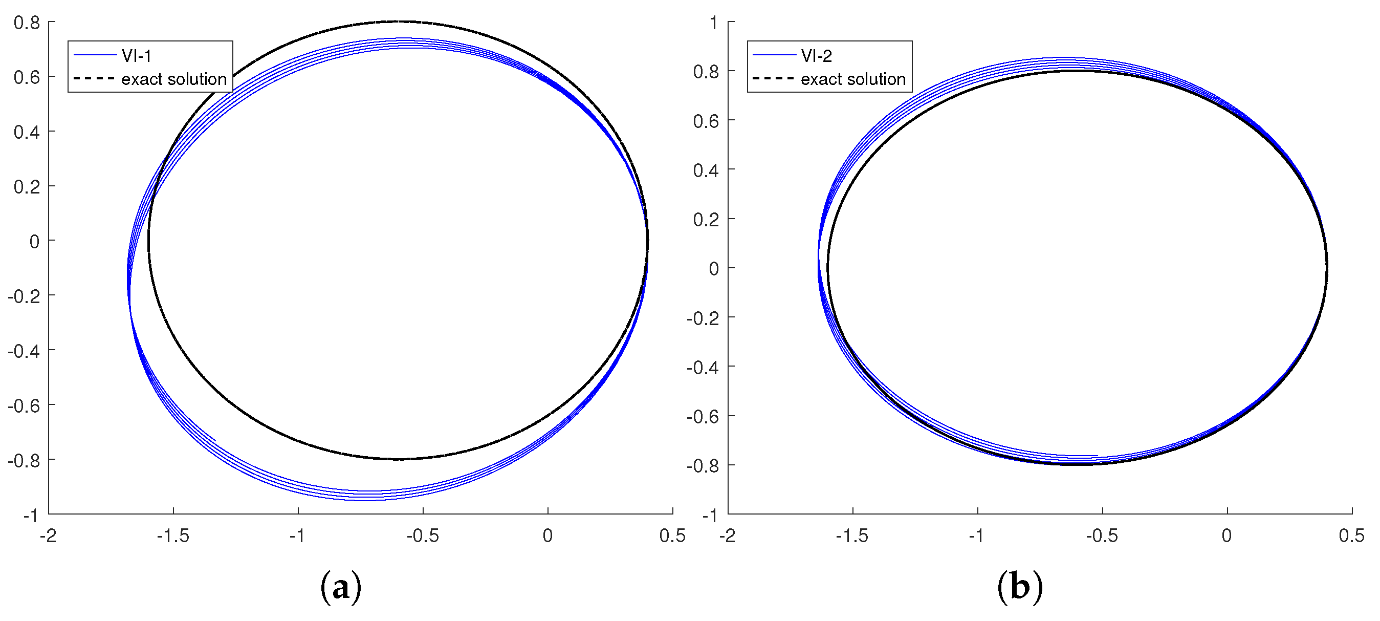
Relativistic Kepler System describes the motion of particles or bodies whose velocities are close to the speed of light. This system can be formulated by introducing proper time, with the Lagrangian given by . The initial conditions are , with a time step of , and the computation spans . In Figure 7, we show the numerical orbits computed by the variational integrators (3.20) and (3.8). The numerical orbits computed by the two variational integrators show better performance qualitatively, confirming the structure-preserving nature of the newly proposed methods in relativistic spacetime.
6. Concluding Remarks
In this paper, we consider a class of second order systems in the form of (2.1), which can describe many important physical problems, including classical mechanics and relativistic plasma dynamics. For this class of systems, we derived the necessary and sufficient conditions for their variational formulation using the basic theory of inverse variational problems. We introduced a class of variational integrators by splitting the Lagrangian and proved that these numerical methods are equivalent to explicit symplectic compositions, ensuring efficient numerical computation. Remarkably, when the newly derived variational integrators are applied to the Kepler problem, we demonstrate better performance compared to the symplectic Euler and Störmer–Verlet methods. To analyze the numerical errors of the variational integrators in preserving conservative quantities, we developed the theory of modified Lagrangians and modified equations. The error estimates in preserving the LRL vector for the Kepler problem verify the numerical behavior. We also simulated the relativistic Kepler problem.
This framework can be extended to PDEs. Consider a nonlinear wave equation with rotational symmetry, assuming the equation has traveling wave solutions of the form , where and . This reduces the wave equation to the following system of second order ODEs:
It can be easily verified that this system satisfies conditions (2.6a)-(2.6b). According to the theorem presented in this paper, this system admits a variational formulation when . This extends the applicability of our approach to various mechanical and continuum problems and opens the door to developing the theory of modified equations for PDEs.
Author Contributions
Conceptualization, Y. Shen and Y. Sun; methodology, Y. Shen and Y. Sun; formal analysis, Y. Shen and Y. Sun; writing—original draft preparation, Y. Shen and Y. Sun; writing—review and editing, Y. Shen and Y. Sun; visualization, Y. Shen; funding acquisition, Y. Sun. All authors have read and agreed to the published version of the manuscript.
Funding
This research was supported by the National Natural Science Foundation of China No. 12271513.
Data Availability Statement
Not applicable.
Conflicts of Interest
The authors declare no conflict of interest.
Abbreviations
The following abbreviations are used in this manuscript:
| PDEs | partial differential equations |
| LRL | Laplace–Runge–Lenz vector |
| Sym-Euler | Symplectic Euler method |
| SV | Störmer–Verlet method |
| VI | Variational integrator |
Appendix A. Modified Equations of Linear Second Order Systems
First, we introduce the basic theory of power series expansion.
Lemma A1.
For , the function has the convergent series expansion
Proof.
Consider the differential equation
By using the polar coordinate transformation with , we have and . Substituting this into (A1) reaches . Thus, with initial conditions and , the solution of (A1) is
Alternatively, we assume can be expressed in a series as
From (A1), the recurrence relation of coefficients follows that , . Solving this gives
The conclusion of this lemma follows by comparing (A2) and (A3). □
Consider the harmonic oscillator
We discretize it by the central difference scheme
The solution of the difference equation (A5) can be expressed as
where a and b are constants determined by the initial conditions. Define , and its second derivative with respect to t is
It is clear that the series on the right-hand side of the above equation converges for .
References
- Feng, K. Collected Works II; National Defense Industry Press: Beijing, 1995. [Google Scholar]
- Hairer, E.; Lubich, C.; Wanner, G. Geometric Numerical Integration, 2nd ed.; Springer-Verlag: Berlin, 2006. [Google Scholar]
- Feng, K.; Qin, M. Symplectic Geometric Algorithms for Hamiltonian Systems; Springer: Heidelberg, 2010. [Google Scholar]
- Vainberg, M.M. Variational Methods for the Study of Nonlinear Operators; Holden-Day: San Francisco, 1964. [Google Scholar]
- Santilli, R.M. Foundations of Theoretical Mechanics I; Springer-Verlag: New York-Heidelberg, 1978. [Google Scholar]
- Olver, P.J. Applications of Lie Groups to Differential Equations, 2nd ed.; Springer-Verlag: New York, 1993. [Google Scholar]
- Marsden, J.E.; West, M. Discrete mechanics and variational integrators. Acta Numer. 2001, 10, 357–514. [Google Scholar] [CrossRef]
- Marsden, J.E.; Pareick, G.W.; Shkoller, S. Multisymplectic Geometry, Variational Integrators, and Nonlinear PDEs. Commun. Math. Phys. 1998, 199, 351–395. [Google Scholar] [CrossRef]
- Sun, Y.; Qin, M. Construction of multisymplectic schemes of any finite order for modified wave equations. J. Math. Phys. 2000, 41, 7854–7868. [Google Scholar] [CrossRef]
- Qin, H.; Guan, X. Variational symplectic integrator for long-time simulations of the guiding-center motion of charged particles in general magnetic fields. Phys. Rev. Lett. 2008, 100, 035006. [Google Scholar] [CrossRef] [PubMed]
- Xiao, J.; Qin, H. Explicit high-order gauge-independent symplectic algorithms for relativistic charged particle dynamics. Comput. Phys. Commun. 2019, 241, 19–27. [Google Scholar] [CrossRef]
- Hairer, E.; Lubich, C. Long-term analysis of a variational integrator for charged-particle dynamics in a strong magnetic field. Numer. Math. 2020, 144, 699–728. [Google Scholar] [CrossRef]
- Hairer, E.; Lubich, C.; Shi, Y. Leapfrog methods for relativistic charged-particle dynamics. SIAM J. Numer. Anal. 2023, 61, 2844–2858. [Google Scholar] [CrossRef]
- Kraus, M.; Maj, O. Variational integrators for nonvariational partial differential equations. Phys. D 2015, 310, 37–71. [Google Scholar] [CrossRef]
- Xiao, J.; Qin, H.; Liu, J. Structure-preserving geometric particle-in-cell methods for Vlasov–Maxwell systems. Plasma Sci. Technol. 2018, 20, 110501. [Google Scholar] [CrossRef]
- Sanz-Serna, J.M. Backward error analysis of symplectic integrators. Fields Inst. Commun. 1996, 10, 193–205. [Google Scholar]
- Hairer, E. Variable time step integration with symplectic methods. Appl. Numer. Math. 1997, 25, 219–227. [Google Scholar] [CrossRef]
- Reich, S. Backward error analysis for numerical integrators. SIAM J. Numer. Anal. 1999, 36, 1549–1570. [Google Scholar] [CrossRef]
- Vermeeren, M. Modified equations for variational integrators. Numer. Math. 2017, 137, 1001–1037. [Google Scholar] [CrossRef]
- Sharma, H.; Borggaard, J.; Patil, M.; Woolsey, C. Performance assessment of energy-preserving, adaptive time-step variational integrators. Commun. Nonlinear Sci. Numer. Simul. 2022, 114, 106646. [Google Scholar] [CrossRef]
- McLachlan, R.I.; Offen, C. Backward error analysis for variational discretisations of PDEs. J. Geom. Mech. 2022, 14, 447–471. [Google Scholar] [CrossRef]
- Oliver, M.; Vasylkevych, S. A new construction of modified equations for variational integrators. arXiv 2024, arXiv:2403.17585. [Google Scholar]
- Chin, S.A. Symplectic integrators from composite operator factorizations. Phys. Lett. A 1997, 226, 344–348. [Google Scholar] [CrossRef]
- Minesaki, Y.; Nakamura, Y. A new discretization of the Kepler motion which conserves the Runge-Lenz vector. Phys. Lett. A 2002, 306, 127–133. [Google Scholar] [CrossRef]
- Minesaki, Y.; Nakamura, Y. A new conservative numerical integration algorithm for the three-dimensional Kepler motion based on the Kustaanheimo-Stiefel regularization theory. Phys. Lett. A 2004, 324, 282–292. [Google Scholar] [CrossRef]
- Kozlov, R. Conservative discretizations of the Kepler motion. J. Phys. A 2007, 40, 4529–4539. [Google Scholar] [CrossRef]
- Arnold, V.I. Mathematical Methods of Classical Mechanics, 2nd ed.; Springer-Verlag: New York, 1989. [Google Scholar]
- Goldstein, H.; Poole, C.P.; Safko, J.L. Classical Mechanics; Pearson Education India, 2011. [Google Scholar]
- Noether, E. Invariante Variationsprobleme. Nachrichten von der Gesellschaft der Wissenschaften zu Göttingen, Mathematisch-Physikalische Klasse, 1918; 235–257. [Google Scholar]
- Vermeeren, M. Numerical precession in variational discretizations of the Kepler problem, Cham, 2018; Vol. 267, Springer Proc. Math. Stat., pp. 333–348.
Figure 1.
Numerical methods and the solutions of truncated modified system
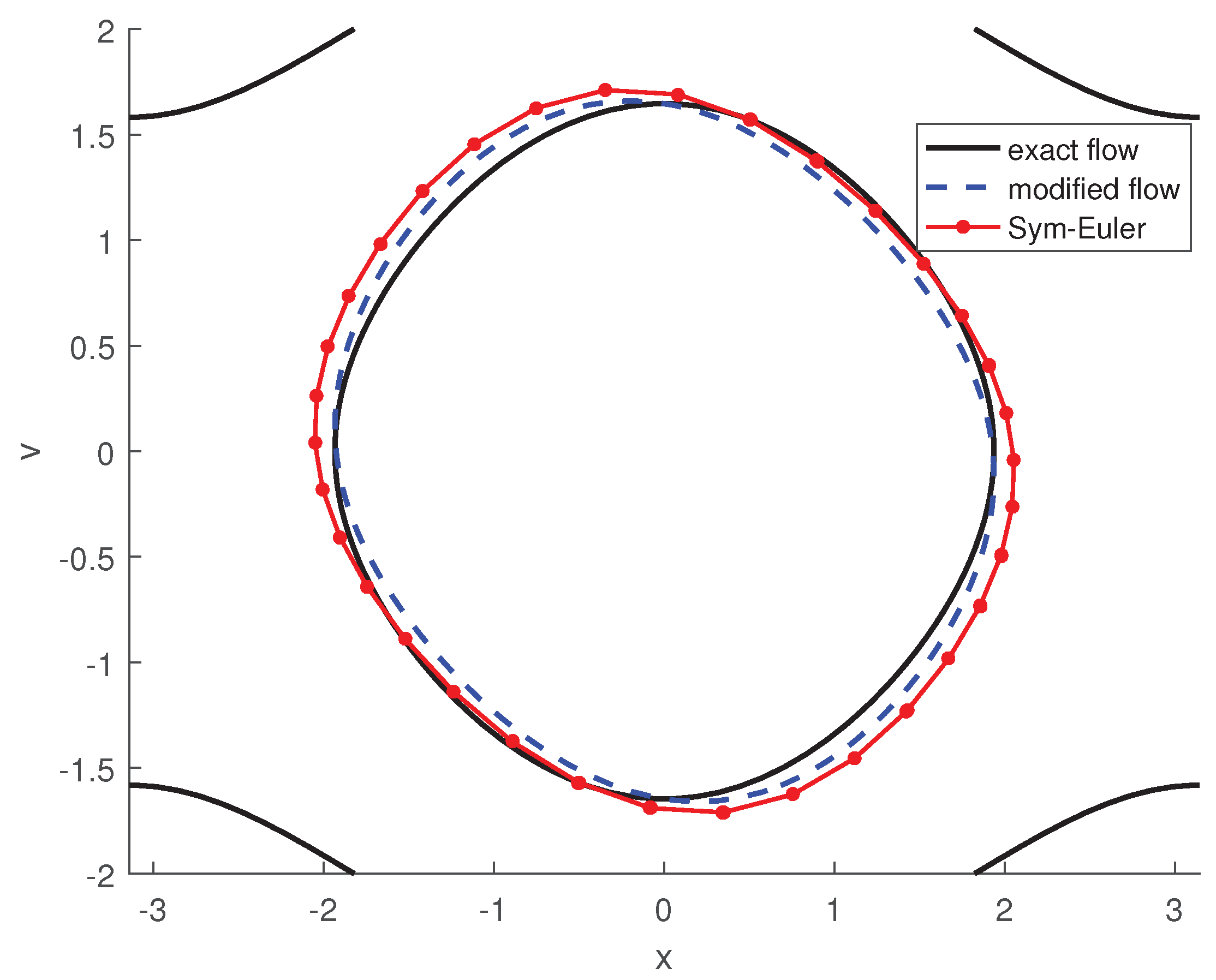
Figure 2.
Keplerian orbits (blue curves) vs exact solutions (red dots) for the Kepler problem
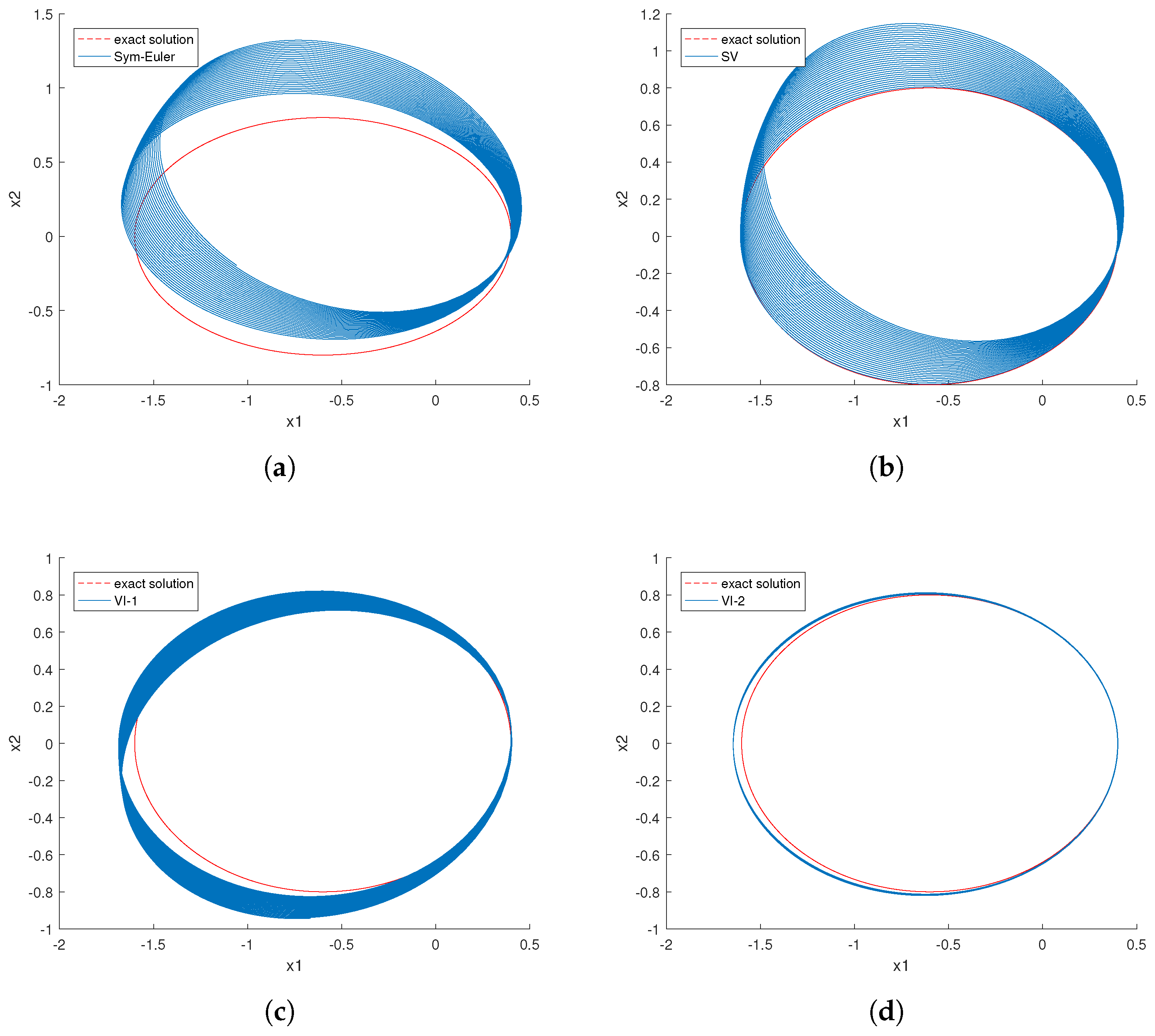
Figure 3.
Energy error. Red: the symplectic Euler and Störmer–Verlet methods; Blue: variational integrators
Figure 3.
Energy error. Red: the symplectic Euler and Störmer–Verlet methods; Blue: variational integrators
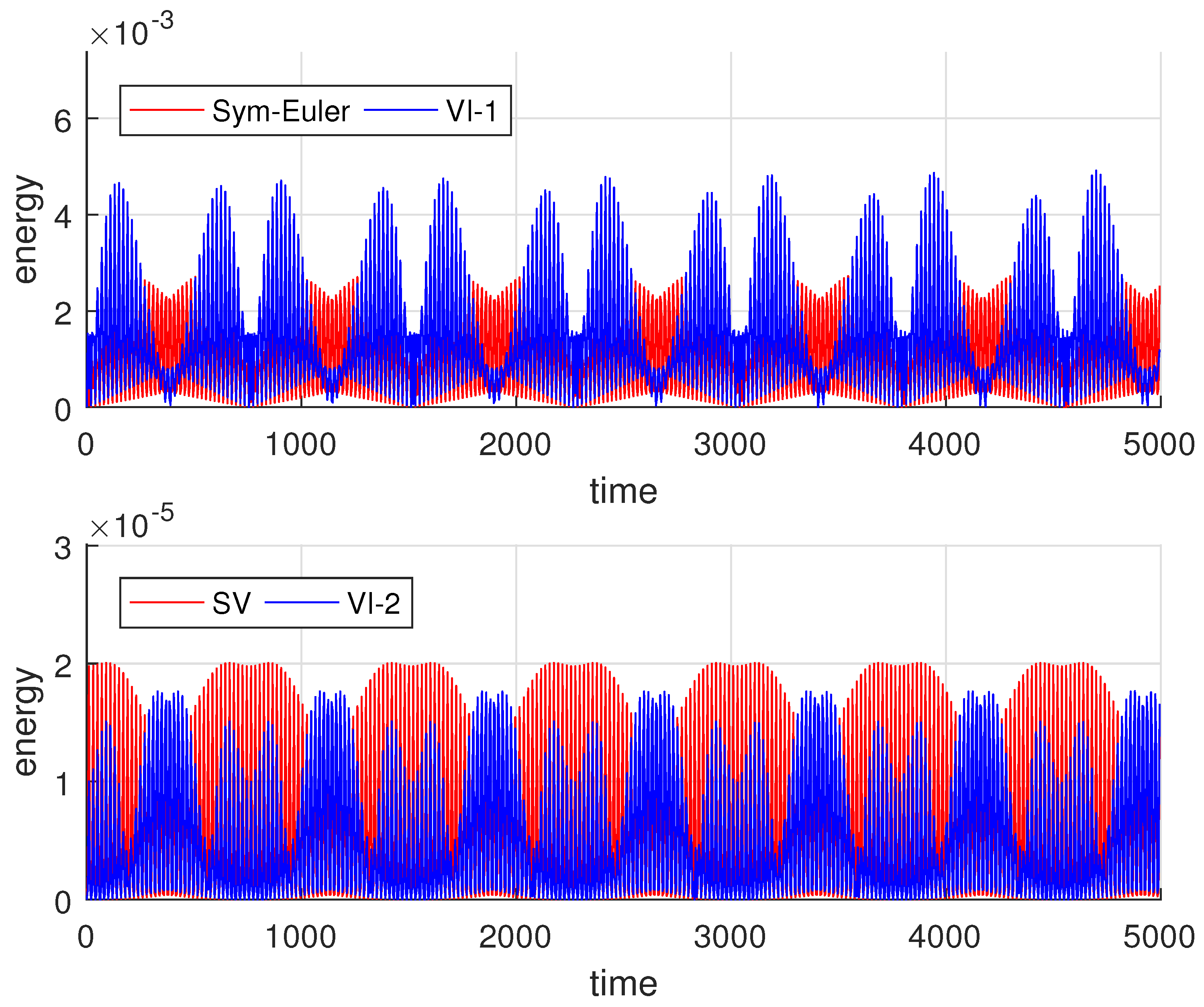
Figure 4.
Eccentricity error. Red: the symplectic Euler and Störmer–Verlet methods; Blue: variational integrators
Figure 4.
Eccentricity error. Red: the symplectic Euler and Störmer–Verlet methods; Blue: variational integrators
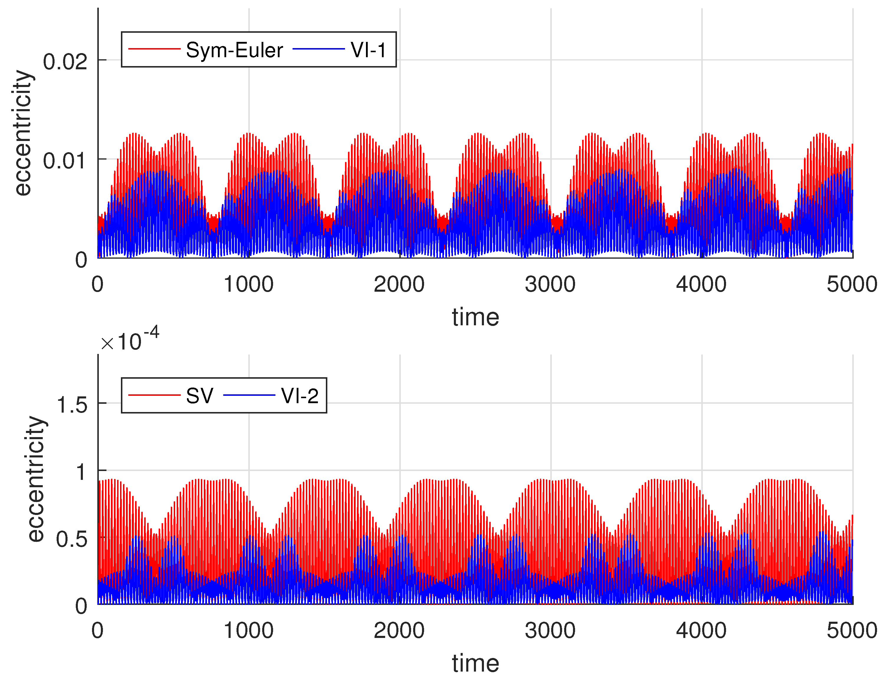
Figure 5.
Rotation angle error. Red: the symplectic Euler and Störmer–Verlet methods; Blue: variational integrators
Figure 5.
Rotation angle error. Red: the symplectic Euler and Störmer–Verlet methods; Blue: variational integrators
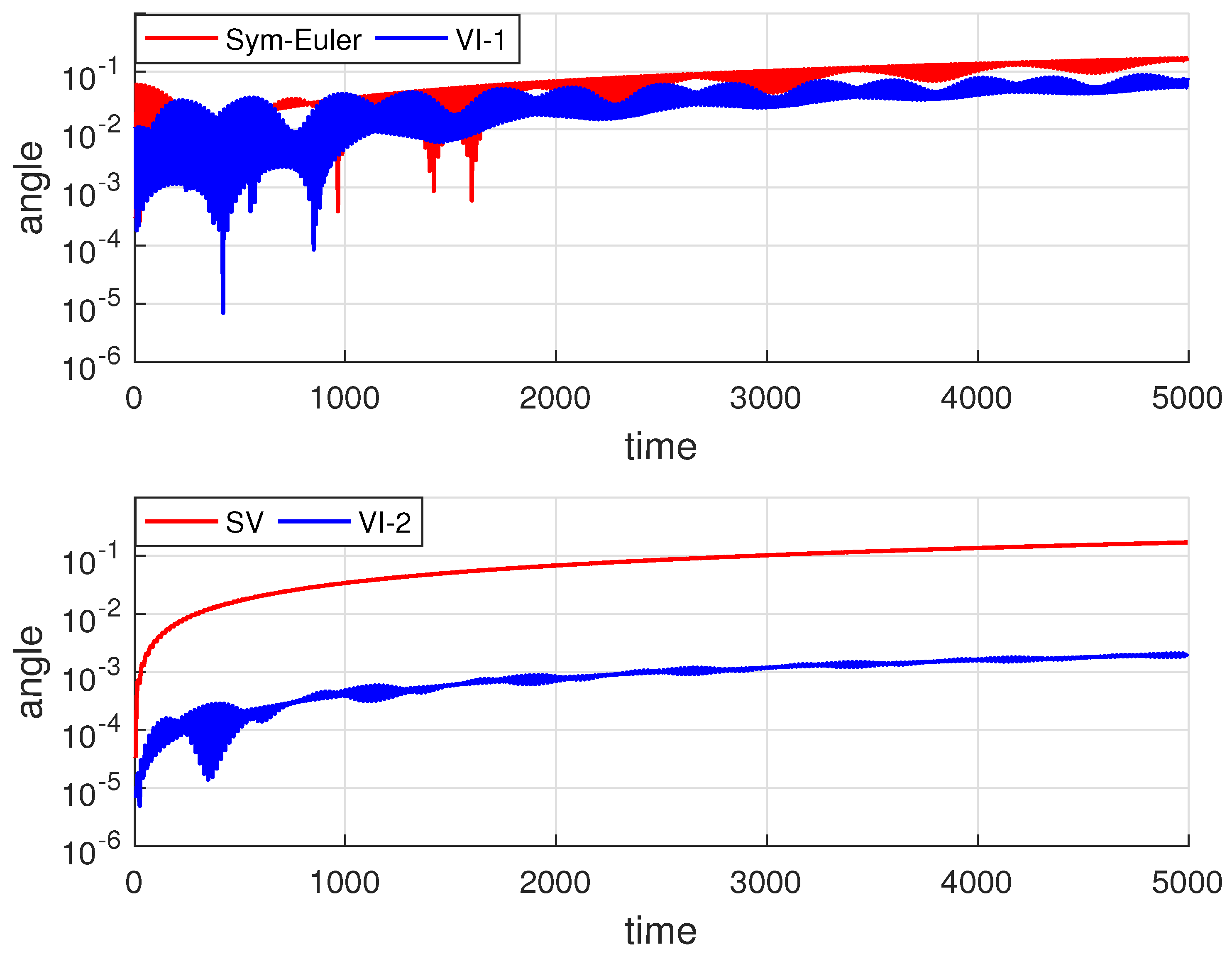
Figure 6.
Convergence rates of the LRL vector over one period of motion. (a) Eccentricity error; (b) Angle error. Solid lines denote the reference convergence rates.
Figure 6.
Convergence rates of the LRL vector over one period of motion. (a) Eccentricity error; (b) Angle error. Solid lines denote the reference convergence rates.
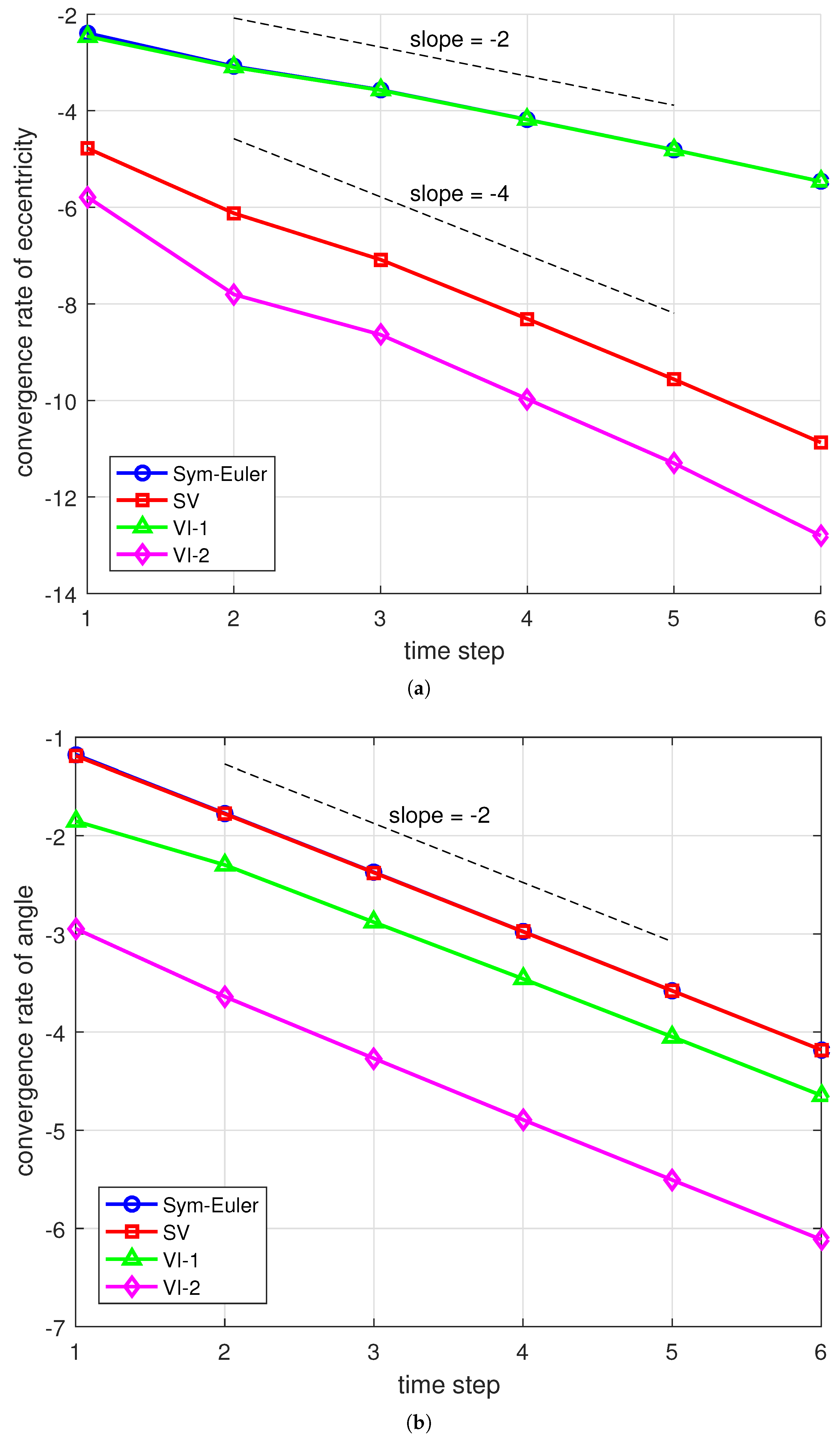
Figure 7.
Numerical solutions from two variational integrators for the relativistic Kepler problem are shown. The blue curves represent the numerical solutions, while the black dots indicate the exact orbits.
Figure 7.
Numerical solutions from two variational integrators for the relativistic Kepler problem are shown. The blue curves represent the numerical solutions, while the black dots indicate the exact orbits.
Disclaimer/Publisher’s Note: The statements, opinions and data contained in all publications are solely those of the individual author(s) and contributor(s) and not of MDPI and/or the editor(s). MDPI and/or the editor(s) disclaim responsibility for any injury to people or property resulting from any ideas, methods, instructions or products referred to in the content. |
© 2025 by the authors. Licensee MDPI, Basel, Switzerland. This article is an open access article distributed under the terms and conditions of the Creative Commons Attribution (CC BY) license (http://creativecommons.org/licenses/by/4.0/).
Copyright: This open access article is published under a Creative Commons CC BY 4.0 license, which permit the free download, distribution, and reuse, provided that the author and preprint are cited in any reuse.


