

Submitted:
06 June 2025
Posted:
06 June 2025
You are already at the latest version
Abstract
This empirical study applies the Sirius Code to the Oklahoma Cash 5 lottery, leveraging the Victoria-Nash Asymmetric Equilibrium (VNAE) to construct a fixed subset strategy using partial coverage with concentrated density. Over 100 consecutive real-world draws, a total of 792 tickets per draw (with m = 12) yielded a net profit of $68,150, or \(6,815 per draw on average. Even with reduced subsets (e.g. m = 10; 252 tickets; net profit of \)35,400 or $354 per draw), the results remained proportionally profitable, in line with the linearity of expectation. The findings suggest that, under certain conditions such as taming some of the true randomness by transforming the “noise” and the “unpredictable” into a strategic game under the lens of game theory and probability theory, it is possible to obtain an asymmetric advantage and consequent sustainable profitability not only for syndicates, but also for individual players.
Keywords:
randomness
; lotteries
; statistics
; game theory
; behavioral economics
; victoria-nash asymmetric equilibrium
Introduction
The pursuit of structural asymmetries within stochastic systems has long fascinated researchers across disciplines. Traditional probabilistic models often treat state-sponsored lotteries as paradigms of pure randomness, where expected losses are embedded by design and profitability is, by definition, unsustainable. However, recent advances in applied probability, game-theoretical framing, and asymmetric equilibrium theory have challenged these assumptions.
This paper applies the Sirius Code, a methodologically self-contained framework previously introduced in Pereira (2025b), to the Oklahoma Cash 5 lottery, a 5/36 draw-based game operated under the Oklahoma Lottery Commission. Unlike systems heavily scrutinized in global financial markets, public lotteries often remain epistemologically sheltered, their randomness culturally unquestioned, their fairness presumed, and their structural design taken as unmanageable.
In this empirical case study, the Sirius Code is used to construct a partial coverage with concentrated density subset of tickets based on the Victoria-Nash Asymmetric Equilibrium (VNAE) principle. This framework enables strategic deviation from uniform random selection while preserving statistical integrity. The dataset comprises 100 consecutive draws, during which the same fixed subset of tickets is repeatedly entered, generating consistent results across multiple payline tiers.
The full derivation of the Sirius Code, its theoretical underpinnings, and the VNAE formulation have been thoroughly explored in previous works (Pereira, 2025a; 2025b). Here, the objective is not to repeat those foundations, but to demonstrate, in action, how these ideas behave when faced with the lived randomness of a public lottery system, and how profit, structure, and signal can emerge even from the most presumed forms of chaos.
1. Methodology
The theoretical foundation for this methodology, the Sirius Code, has been thoroughly developed in Pereira (2025), to which the reader is referred for a comprehensive mathematical treatment. The Oklahoma Cash 5 lottery, operated in the United States, was selected as a representative example of 5/36 lottery designs. As in previous studies involving the Sirius Code, the analysis is based on 100 consecutive real-world draws. In this case, following the same approach adopted in the UK 6/59 Lotto study, the 100 most recent draws were considered, beginning from the moment the author initiated the analysis and documentation of this material. As a means of evaluating long-term performance, the results were assessed through the cumulative relationship between profit and loss across each individual draw.
2. Results and Discussions
2.1. Dicing in the Name: Oklahoma Cash 5
The Oklahoma Cash 5 is a state-operated lottery game structured around a 5/36 matrix format. Participants are required to select five distinct numbers from a fixed set of integers ranging from 1 to 36. Drawings occur daily, with prize tiers awarded based on the number of matches between the selected ticket and the official draw. Unlike games with progressive jackpots or complex multiplicative prize structures, Cash 5 offers a relatively stable, deterministic payout model across three tiers (3, 4, and 5 matches), with a fixed jackpot for a five-number match.
Table 1 shows the prize tiers with their respective payoffs and probabilities:
In this study, further detailed in Pereira (2025b) and Pereira (2025a), we employ the method of partial coverage with concentrated density using m = 12. Specifically, in an alternative lottery setup, we select a subset of 5 numbers drawn from the integers 1 to 12 and purchase all possible combinations within that subset.
For the sake of simplification, we assume that the chosen subset comprises the first 12 numbers (which we may refer to as “correct matches” or “successes” if any are drawn). All other numbers are disregarded in our analysis; if the draw includes any number outside our optimized subset, it is classified as a “miss” or “failure.” In practice, any other set of 12 numbers could be used, as the process is inherently stochastic, with uniformity and independence among the elements of the sample space.
Table 2 presents the total number of possible combinations for m = 12, which amounts to 792. These combinations are subsequently categorized according to the different ranges of matching outcomes.
As observed in Table 2, among the 792 possible combinations, 35 tickets contain exactly 4 matching numbers, each yielding a prize of $500. Similarly, combinations with only 2 correct numbers are eligible for a free ticket, which serves as a relevant mechanism for mitigating losses over the medium to long term.
Table 3 outlines the cost-benefit dynamics as distributed across various prize categories:
With only one or no matching numbers, the entire set of 792 tickets results in a complete loss. However, even with just two correct numbers, the model begins to show signs of scalability, particularly if the convergence of probabilities tends, even in the worst-case scenarios, toward at least two matches rather than none or only one. From three correct numbers onward, we already observe a satisfactory net profit of $1,308. Moreover, it is the tier of four matches that ultimately drives the expected value into positive territory.
2.2. Just Know We Mean It
Next, we will analyze a historical series of 100 draws of the Oklahoma Cash 5:

Table 4.
Oklahoma Cash 5 Lotto results with m = 12 (Part I).
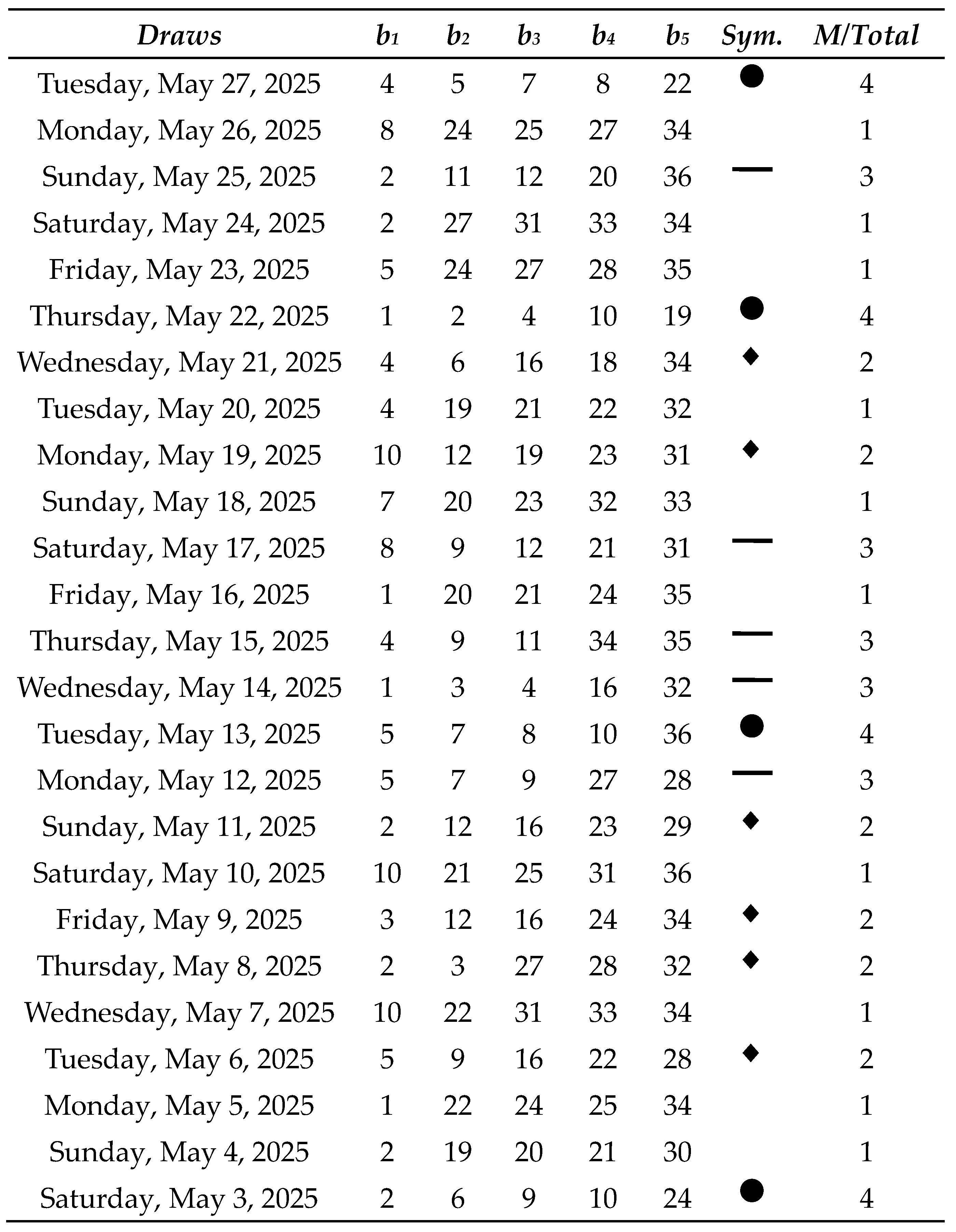
Table 5.
Oklahoma Cash 5 Lotto results with m = 12 (Part II).
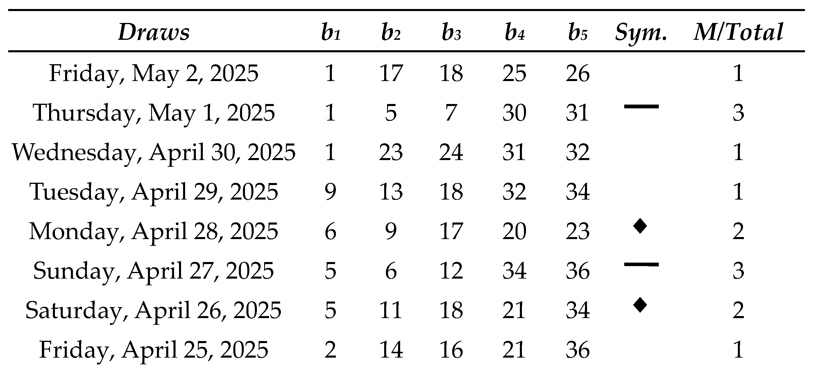
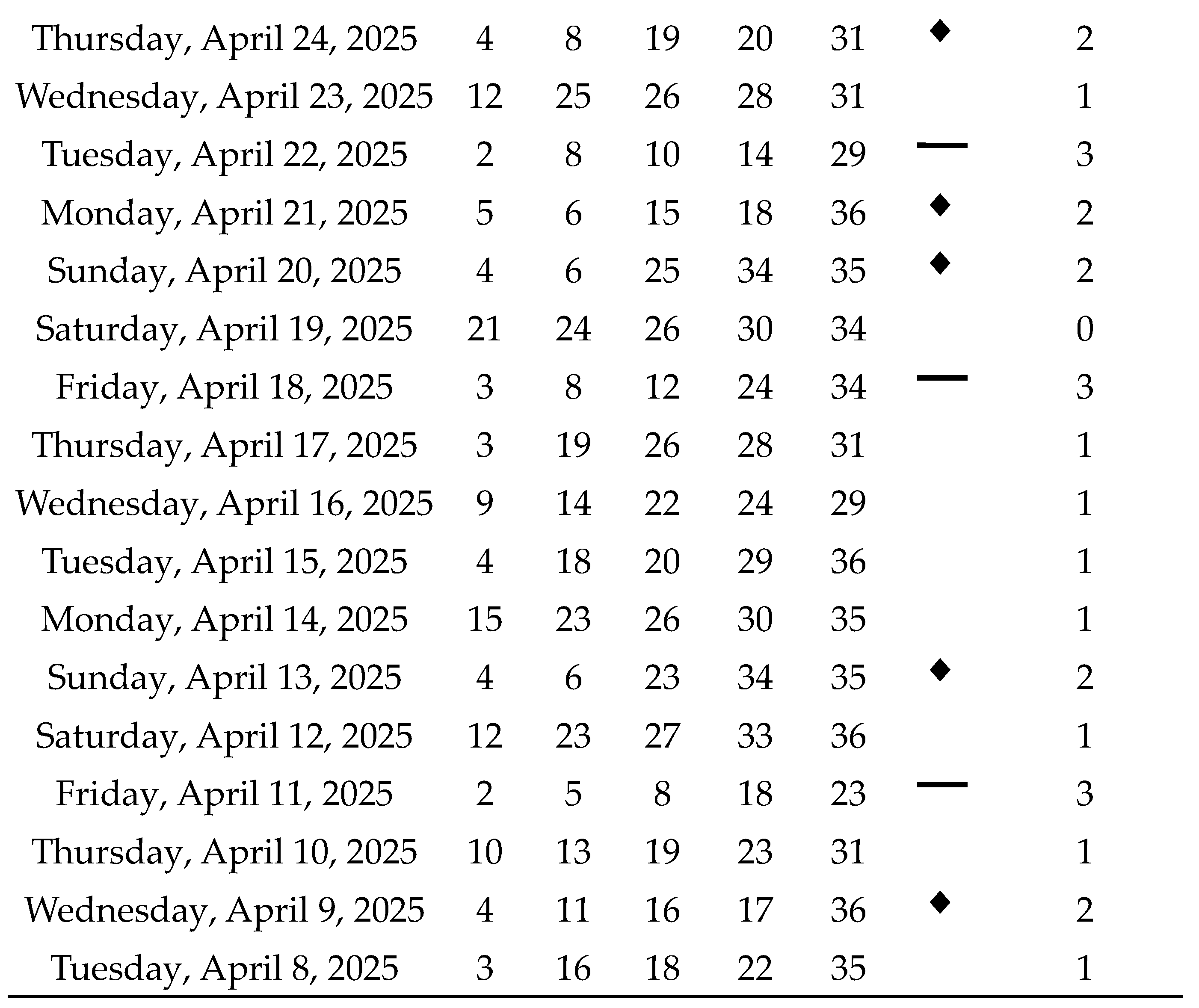
Table 6.
Oklahoma Cash 5 Lotto results with m = 12 (Part III).
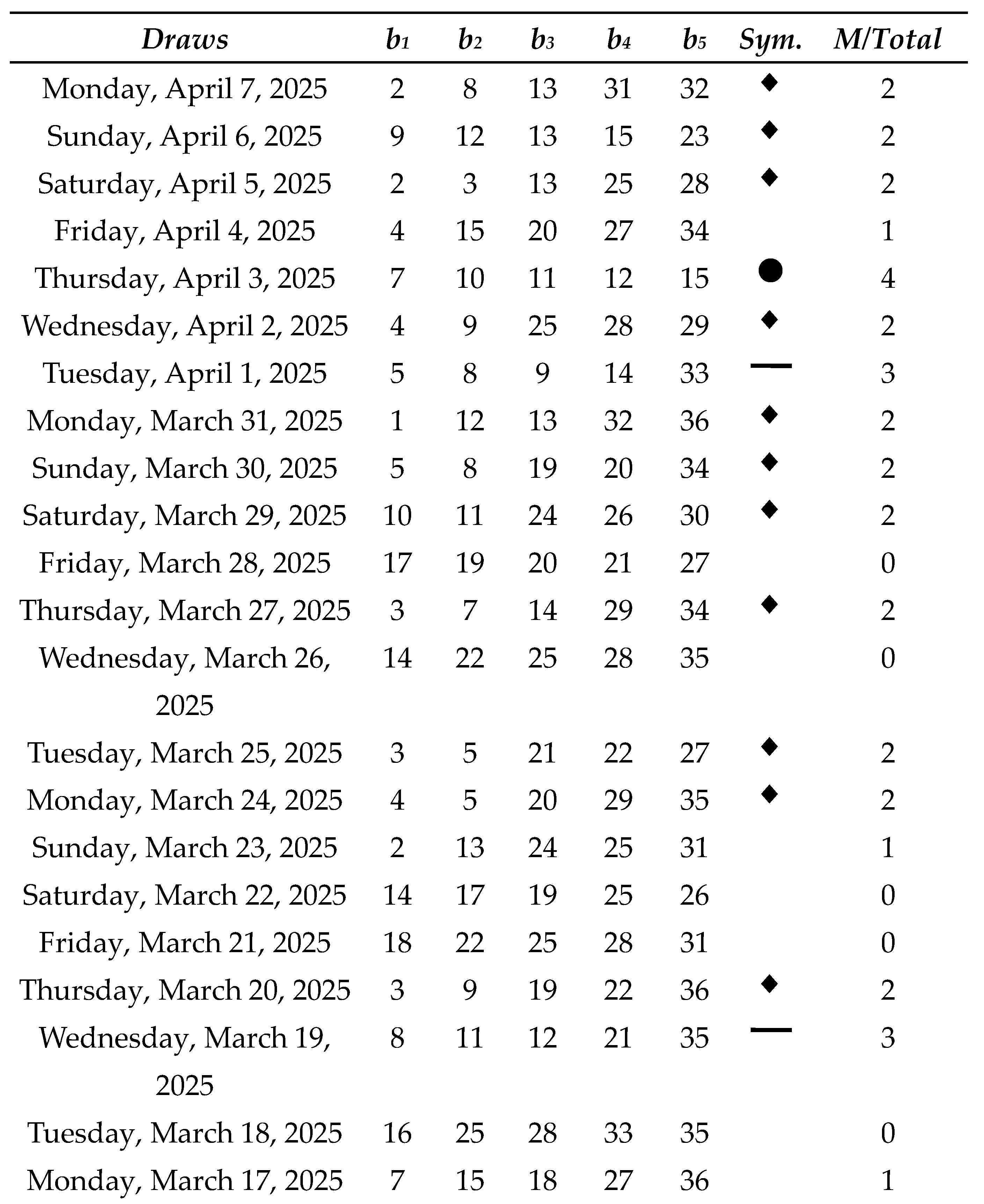

Table 7.
Oklahoma Cash 5 Lotto results with m = 12 (Part IV).
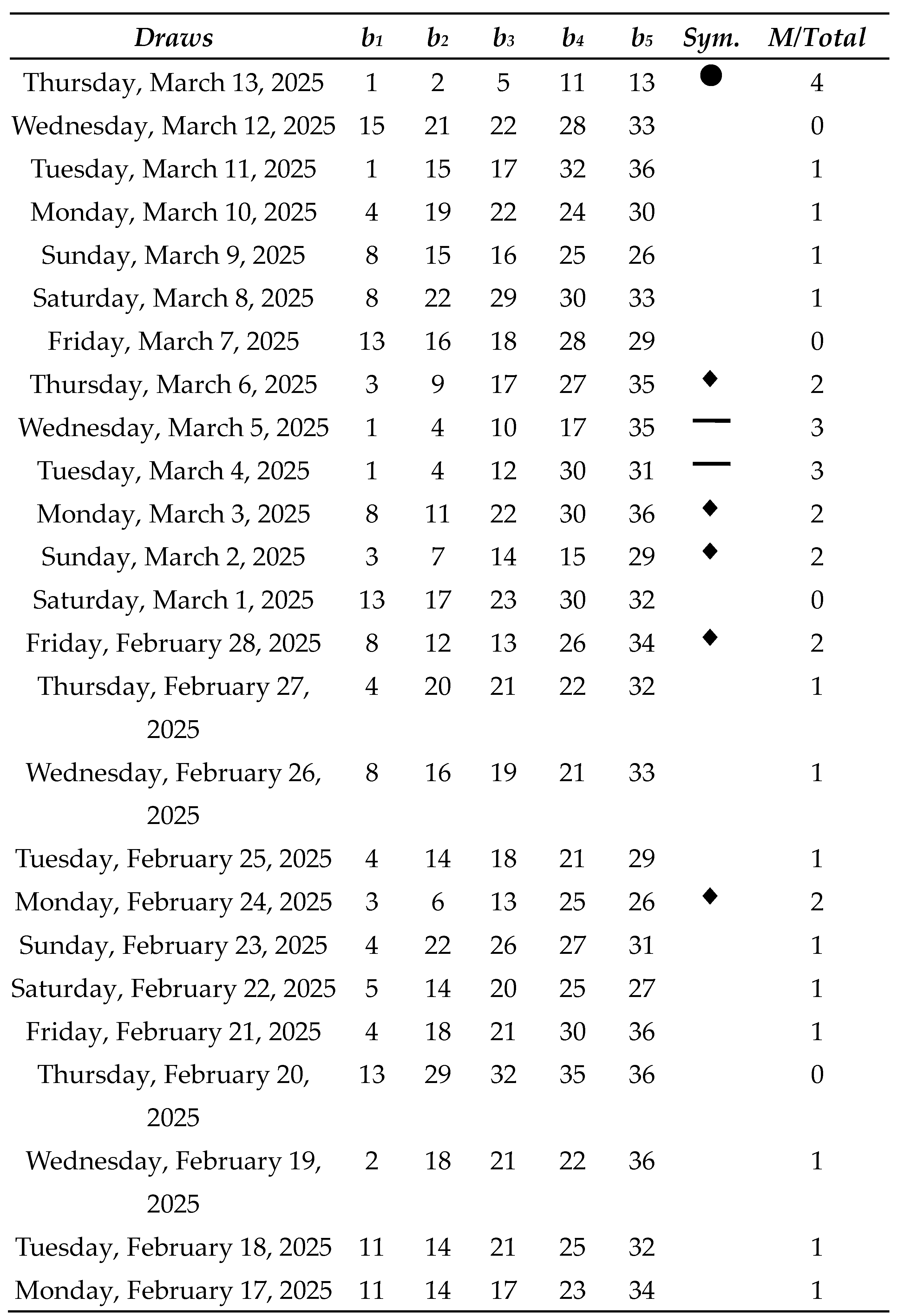
Table 8 shows all the matches we had in this simulation with real data from Oklahoma Cash 5, as well as the sum of the net results for each match range:
As a result, a net profit of $68,150 was achieved over the course of 100 consecutive draws, corresponding to an average profit of $6,815 per draw under the partial coverage with concentrated density using m = 12, which requires the purchase of 792 tickets per individual draw. Further reductions in the number of tickets are feasible; however, profits tend to scale proportionally, in accordance with the principle of linearity of expectation. For instance, if only 10% of the 792 preselected combinations were employed, that is, 79 tickets per draw, the expected net return would be approximately $68.15 per draw. Thus, the Sirius Code proves to be a viable strategy not only for lottery syndicates but also for individual players.
It should be made clear that this study is not intended to generalize in the sense that every 100 draws will give us something in the way of profit. However, the indications are very strong that we have a reasonably positive mathematical expectation of a profit in every 100 draws in this lottery design.
If we consider a scenario with m = 10, that is, selecting all possible combinations of 5 numbers drawn from a subset of 1 to 10 in an ‘alternative lottery’, we would need to purchase only 252 tickets per draw, as opposed to covering all 376,992 possible combinations aimed at the jackpot, which, in this particular lottery format, is arguably not especially attractive. With only 0.07% of the total combination space “covered,” we are nonetheless inclined by Pereira’s (2025c) Victoria-Nash Asymmetric Equilibrium (VNAE); Law of Large Numbers; and Chebyshev’s inequalities to secure a positive expected value. Using the same historical data, we arrive at the following results:
Table 9.
Number of winning tickets by match category under the partial coverage with concentrated density with m = 10.
Table 9.
Number of winning tickets by match category under the partial coverage with concentrated density with m = 10.
| Matches | N° of Success Tickets | Expected Prize |
|---|---|---|
| 5 | 1 | $25,000 |
| 4 | 25 | $500 |
| 3 | 100 | $10 |
| 2 | 100 | Free Ticket |
Table 10.
Cost-benefit analysis by match category under the partial coverage with concentrated density with m = 10.
Table 10.
Cost-benefit analysis by match category under the partial coverage with concentrated density with m = 10.
| Matches | Prizes - Costs |
|---|---|
| 5 | $24,748 |
| 4 | $12,248 |
| 3 | $748 |
| 2 | -$152 |
| X ≤ 1 | -$252 |
Table 11.
Analysis of 100 Oklahoma Cash 5 Lotto draws considering partial coverage with concentrated density with m = 12.
Table 11.
Analysis of 100 Oklahoma Cash 5 Lotto draws considering partial coverage with concentrated density with m = 12.
| Matches | 100 Last Draws | P/L |
|---|---|---|
| 5 | - | - |
| 4 | 4 | 48,992 |
| 3 | 8 | 5,984 |
| 2 | 26 | -$3,952 |
| X ≤ 1 | 62 | -$15,624 |
| 100 | $35,400 |
As demonstrated with m = 10, selecting all 252 possible combinations from the first 10 numbers out of the full 1-36 range would have yielded a net profit of $35,400 across 100 consecutive draws averaging $354 per draw. If we were to further reduce the number of tickets, employing only 10% of this optimized subset (i.e., 25 tickets), we would still observe a proportionally scaled return of approximately $35.40 per draw, albeit with increased variance and standard deviation due to the smaller sample size.
2.3. Analysis of an Additional Historical Series
As a complementary analysis - open to verification by the academic community through the official Oklahoma Cash 5 results platform or sources such as Lottery Post - we present an additional historical series comprising 100 draws, this time covering an earlier period than the one previously analyzed. Specifically, the draws span from November 9, 2024 to February 16, 2025, and apply the same methodology with m = 12. The results obtained are as follows:
Table 12.
Analysis of an additional series of 100 Oklahoma Cash 5 Lotto draws considering partial coverage with concentrated density with m = 12.
Table 12.
Analysis of an additional series of 100 Oklahoma Cash 5 Lotto draws considering partial coverage with concentrated density with m = 12.
| Matches | 100 Last Draws | P/L |
|---|---|---|
| 5 | - | - |
| 4 | 5 | $83,540 |
| 3 | 20 | $26,160 |
| 2 | 31 | -$13,702 |
| X ≤ 1 | 44 | -$34,848 |
| 100 | $61,150 |
The results indicate that, over the course of 100 consecutive draws, the strategy would have achieved 4-out-of-5 matches in 5 instances and 3-out-of-5 matches in 20 instances. This would have resulted in a net profit of $61,150, equivalent to an average of $611.50 per draw, using only 792 tickets per draw. These outcomes suggest that the observed profitability is not merely a product of overfitting or sampling bias.
2.4. What Goes Around Comes Around
Although previously noted, in contrast to earlier studies, this real-world case study also employs specific symbols as a means to enhance the visualization of results across different ranges of correct matches, aiming to clarify and make more intelligible the convergence effect in probabilities within uniformly distributed random events. As can be observed, no symbols were assigned to the ranges r = 0 and r = 1 correct matches, as highlighting losses is not, in principle, of interest in the current analysis. The range r = 2 correct matches, on the other hand, is represented by a rhombus symbol, as it corresponds to smaller losses that occur with notable frequency but not to an extent that would induce a negative long-term trend.
If we consider the Law of Large Numbers and Chebyshev’s inequalities, and hypothetically ‘accept’ that the mean does in fact converge such that achieving exactly 4 correct matches in 100 consecutive draws occurs in approximately 5 or 6 instances, as observed by Pereira (2025b), one may reasonably infer that there is insufficient rationale to proceed with the remaining 75 draws. This is because a substantial portion of the potential profit has already been captured within the first 25 draws (amounting to $62,800), rendering the remaining 75 draws comparatively less attractive and unconvincing from a profitability standpoint, essentially amounting to a disproportionate expenditure of energy for an additional gain of ‘merely’ $5,350.
Conclusions
The empirical results demonstrate that, under a partial coverage with concentrated density guided by the Sirius Code and the Victoria-Nash Asymmetric Equilibrium, positive expected returns are consistently achievable, even within systems presumed to be mathematically “unbeatable” and purely random. The structure is not only resilient to reduction in ticket volume but also scalable across varying levels of participation.
Rather than offering guarantees of profit in every single draw, this study suggests a deeper principle: when the “architecture of randomness” is properly aligned with probability theory, it can tilt long-term outcomes in favor of the player. In the end, even the fairest dice may roll with a pattern if only one dares to ‘tame’ and choreograph the chaos. Again, it was a good dice.
References
- Pereira, Daniel Henrique, Application of the Sirius Code to UK 6/59 Lotto: An Empirical Analysis of Asymmetric Equilibrium and Sustainable Profitability (2025a). Available at SSRN: https://ssrn.com/abstract=5277977. [CrossRef]
- Pereira, Daniel Henrique, Sirius Code: Leveraging the Victoria-Nash Asymmetric Equilibrium for Sustainable Lottery Profits (2025b). Available at SSRN: https://ssrn.com/abstract=5264192. [CrossRef]
- Pereira, Daniel Henrique, Victoria: Beating the House Using the Principles of Statistics and Randomness (2025c). Available at SSRN: https://ssrn.com/abstract=5209733. [CrossRef]
Table 1.
Expected prize values by prize tier (based on number of r matches).
| Matches | Expected Mean | Odds |
|---|---|---|
| r = 5 | $25,000 | 1 in 376,992 |
| r = 4 | $500 | 1 in 2,434.2 |
| r = 3 | $10 | 1 in 81.1 |
| r = 2 | Free Ticket | 1 in 8.4 |
Table 2.
Number of winning tickets by match category under the partial coverage with concentrated density with m = 12.
Table 2.
Number of winning tickets by match category under the partial coverage with concentrated density with m = 12.
| Matches | N° of Success Tickets | Expected Prize |
|---|---|---|
| 5 | 1 | $25,000 |
| 4 | 35 | $500 |
| 3 | 210 | $10 |
| 2 | 350 | Free Ticket |
Table 3.
Cost-benefit analysis by match category under the partial coverage with concentrated density with m = 12.
Table 3.
Cost-benefit analysis by match category under the partial coverage with concentrated density with m = 12.
| Matches | Prizes - Costs |
|---|---|
| 5 | $24,208* |
| 4 | $16,708 |
| 3 | 1,308 |
| 2 | -$442 |
| X ≤ 1 | -$792 |
Table 8.
Analysis of 100 Oklahoma Cash 5 Lotto draws considering partial coverage with concentrated density with m = 12.
Table 8.
Analysis of 100 Oklahoma Cash 5 Lotto draws considering partial coverage with concentrated density with m = 12.
| Matches | 100 Last Draws | P/L |
|---|---|---|
| 5 | - | - |
| 4 | 6 | $100,248 |
| 3 | 15 | $19,620 |
| 2 | 31 | -$13,702 |
| X ≤ 1 | 48 | -$38,016 |
| 100 | $68,150 |
Disclaimer/Publisher’s Note: The statements, opinions and data contained in all publications are solely those of the individual author(s) and contributor(s) and not of MDPI and/or the editor(s). MDPI and/or the editor(s) disclaim responsibility for any injury to people or property resulting from any ideas, methods, instructions or products referred to in the content. |
© 2025 by the authors. Licensee MDPI, Basel, Switzerland. This article is an open access article distributed under the terms and conditions of the Creative Commons Attribution (CC BY) license (http://creativecommons.org/licenses/by/4.0/).
Copyright: This open access article is published under a Creative Commons CC BY 4.0 license, which permit the free download, distribution, and reuse, provided that the author and preprint are cited in any reuse.


