Submitted:
03 June 2025
Posted:
04 June 2025
You are already at the latest version
Abstract
Cancer remains one of the most significant global health challenges due to its high mortality rates and the limited understanding surrounding its progression. Early diagnosis is critical to improving patient outcomes, especially for skin cancer, where timely detection can dramatically enhance recovery rates. Histopathological analysis is a common diagnostic method for skin cancer, but it is a cumbersome process that relies heavily on the expertise of highly trained specialists. Recent advancements in Artificial Intelligence have demonstrated promising results in image classification tasks, suggesting its potential as a support tool for medical diagnosis. This study explores applying hybrid models for melanoma diagnosis using histopathological images. We propose a two-step framework that leverages an Autoencoder for dimensionality reduction and feature extraction, followed by a classification algorithm for melanoma-nevi discrimination, where we tested Support Vector Machines, Random Forest, Multilayer Perceptron, and K-Nearest Neighbours. Among the models evaluated, the Autoencoder combined with K-Nearest Neighbours or Random Forest achieved the best performance, with an accuracy of approximately 97.95%.
Keywords:
hybrid models
; deep learning
; machine learning
; diagnostic models
; skin cancer
; melanoma
1. Introduction
Cancer is widely recognised as one of the most challenging diseases for physicians, due to its multifactorial complexity. Its genetic nature, rooted in DNA mutations and alterations, leads to high heterogeneity across cases. Additionally, environmental factors significantly influence tumour growth and progression, further complicating its diagnosis and treatment. Also, the variability in individual responses to cancer requires the adoption of personalised therapeutic approaches. Moreover, cancer requires a multidisciplinary approach, involving the collaboration of oncologists, surgeons, pathologists, and other specialists to provide comprehensive care. The diversity of cancer types adds another layer of complexity, with over 200 distinct forms identified regarding (Kaya et al. 2022), each demanding specialised expertise for proper diagnosis and treatment. Among these, skin cancer stands out as one of the most common forms in the United States, with its global prevalence continuing to rise, (Woo et al. 2022). Addressing this growing challenge requires significant efforts to advance diagnostic and therapeutic strategies tailored to the unique nature of skin cancer and its subtypes.
The most severe and potentially life-threatening form of skin cancer is melanoma. (Siegel, Miller, and Jemal 2019) points out that in the United States, it is ranked as the fifth most common cancer in both men and women. It accounts for approximately 350,000 new cases and 57,000 deaths reported globally in 2020, (Arnold et al. 2022). The incidence increases with age, underscoring the importance of monitoring the population as it grows older. Survival rates for melanoma are closely linked to the stage of the disease at the time of diagnosis, making early detection a critical factor in improving patient outcomes and saving lives. While many melanomas are initially detected by patients themselves (Carli et al. 2003), clinician detection is often associated with thinner, more treatable tumours (Swetter et al. 2009). This highlights the value of professional screening in identifying melanomas at an early stage. For patients diagnosed with thin lesions and invasive melanomas (Breslow thickness ≤1 mm), treatment typically results in prolonged disease-free survival and, in most cases, a complete cure, (Green et al. 2012).
The current gold standard for melanoma diagnosis is histopathology, which analyses melanocytic neoplasms. These areas are tumours that originate from melanocytes, which are the cells responsible for producing the pigment in the skin. However, a subset of these neoplasms cannot be unequivocally classified as benign (nevus) or malignant (melanoma). These ambiguous cases are a significant source of diagnostic error, as evidenced by studies reporting discordance rates between expert dermatopathologists ranging from 14% to 38% using routine examination (Shoo, Sagebiel, and Kashani-Sabet 2010). To reduce the risk of missing malignant lesions, the diagnostic criteria for melanoma have been adjusted to emphasise detecting as many potential cases as possible (sensitivity), even if this comes at the expense of a higher false positive rate (reduced specificity). This trade-off highlights the urgent need for diagnostic tests that can increase accuracy by providing quantitative, objective information to minimise the inherent subjectivity of histopathological evaluation. Genetic analyses of melanocytic lesions have shown promise in distinguishing melanomas that harbour recurrent genetic aberrations absent in unequivocally benign lesions (Bastian et al. 2003). However, a “grey area” remains histologically ambiguous melanocytic neoplasms with few genetic aberrations that continue to pose uncertainty regarding their biological behaviour. In this way, Artificial intelligence (AI) techniques present a compelling solution to this problem.
By analysing big datasets, AI models can identify patterns in cases that are critical for human interpretation. These models can deliver diagnoses automatically and with remarkable speed, offering significant help in the accuracy and efficiency of melanoma diagnosis. AI is a discipline that aims to understand and replicate the mechanisms underlying intelligent behaviour in machines. This is achieved through various methods, which do not necessarily mimic the original biological mechanisms. AI encompasses a wide range of approaches, with Machine Learning (ML) being the most prominent in recent years. As defined by (Samuel 1959), ML is a field of study that enables computers to learn autonomously without explicit programming. It includes numerous techniques, where Deep Learning (DL) has emerged as a groundbreaking advancement. Deep Learning, as described by (LeCun, Bengio, and Hinton 2015), refers to models capable of learning hierarchical representations of data through multiple levels of abstraction. These models are inspired by artificial neural networks, designed to emulate the behaviour of biological neurons. They achieve this through interconnected layers arranged sequentially, enabling them to process complex patterns and relationships within data effectively.
The primary motivation of this study is to develop a fast and accurate approach for diagnosing melanoma using histopathological images, aiming to speed up the diagnostic process for physicians. The proposed methods address the challenges associated with the high dimensionality of histopathological images, which require significant computational resources and complex feature extraction. To tackle these issues, we leverage the advantages of Autoencoders for enhanced feature extraction by reducing the dimensionality, combined with classical machine learning models for classification. Furthermore, the study incorporates a subjective evaluation to better understand the model’s performance and to identify common histopathological features that might confuse the classifier during diagnosis. This evaluation aims to bridge the gap between automated diagnostic tools and clinical practice, offering valuable insights to improve both the performance of the model and its interpretability for medical professionals.
The contribution of this work lies in the development of a workflow that first employs an Autoencoder for dimensionality reduction and feature extraction from histopathological images, followed by using these extracted features with various classifiers. This workflow produces hybrid models that integrate novel Deep Learning techniques with classical Machine Learning algorithms. The performance of these hybrid combinations is evaluated both objectively, using standard mathematical metrics, and subjectively, through the insights of a medical expert in the field.
The innovation of the paper consists of the presented workflow and the different hybrid models, which, as far as we know, is the first time that these combinations are applied to diagnose melanoma using histopathological images. Also, the subjective evaluation lets us understand how the model works and what its limitations are.
The remaining sections of the paper are structured as follows. Section 2 provides a compilation of previous papers that pertain to the same field or share similarities with the proposed work. In Section 3, the data utilized for training the models and addressing the problems are described in detail. Section 4 presents the research findings and showcases the results obtained through the course of the study. Finally, Section 5 offers concluding remarks and highlights potential avenues for future research.
2. Related works
As said above, in this work different hybrid models using deep learning models alongside classical machine learning techniques have been proposed to diagnose melanoma with histopathologic images. Following, we compile different works using similar techniques for skin cancer diagnosis in general or melanoma.
First, we compile some works that only use classical machine learning techniques. (Thepade and Ramnani 2021) uses Haar wavelet transformation in dermoscopy skin images to extract the main feature. These features are, then, introduced in different classifiers using random forest algorithm, Support Vector Machines (SVM), or Naïve Bayes to discriminate between benign and malignant lesions. The same dataset is used in (Murugan, Nair, and Kumar 2019) where preprocessing techniques are used to eliminate noise and occlusion, such as body hairs. Then, some characteristics were obtained by applying the ABCD rule and using them to feed different ML models like SVM, random forests, and K-Nearest Neighbours (KNN). Another type of image to diagnose skin cancer is Optical Coherence Tomography (OCT), which is used by (Liu et al. 2014) to acquire both intensity and birefringence images of healthy and cancerous mouse skin samples. Using an SVM-based classifier, the researchers aimed to automatically distinguish images indicative of basal cell carcinoma (BCC), the most common type of skin cancer. Vibrational OCT is used with logistic regression and SVM to use telemedicine to classify between basal cell carcinoma (BCC), squamous cell carcinoma (SCC), melanoma, and controls, (Silver et al. 2023). In (Mishra et al. 2022) Different preprocessing techniques, including the Gray Level Co-Occurrence Matrix (GLCM), Principal Component Analysis (PCA), and fuzzy C-means clustering, extract features from skin cancer images, and then utilise SVM for diagnosis. Also, (Brorsen et al. 2024) integrates Matrix-Assisted Laser Desorption/Ionization Mass Spectrometry Imaging (MALDI-MSI) with Logistic Regression (LR) to characterize and delineate cutaneous squamous cell carcinoma, achieving a predictive accuracy of 92.3% in cross-validation. Finally, (Mosquera-Zamudio et al. 2024) applies Gaussian Naïve Bayes (GNB) and Logistic Regression (LR) to improve the histological classification of spitzoid tumours using Whole Slide Images (WSI) and clinicopathological features. To the best of our knowledge, the latter is the only work that utilises histopathological images in conjunction with classic machine-learning algorithms, although its primary aim is not melanoma diagnosis. In our case, we are not only using our dataset of histopathologies in melanoma, but we are also creating hybrid models that, apart from ML models, are using DL ones that face the problem of high dimensionality in this kind of image.
In the case of the DL models used to diagnose skin cancer, we have the following works. (Gouda et al. 2022) uses different preprocessing techniques in images of skin lesions and evaluates how different CNN models (Resnet50, InceptionV3, and Inception Resnet) performed in diagnosing and classifying. Another work using CNN models is (Kousis et al. 2022) where 11 different architectures were trained with a dataset that comprises 7 different skin lesions. After obtaining a model that performs well, it was also able to inform about the duration of sun exposure depending on the current UV radiation level, the individual’s skin phototypes, and the level of protection provided by the sunscreen used. Another CNN model is applied in (Shorfuzzaman 2022), adding a shapely adaptive method to explain the diagnosis of melanoma through a heatmap. In the case of deep learning, papers are using histopathologic images. In (Wako et al. 2022) different pre-trained models like EfficientNetB0, MobileNetv2, ResNet50, and VGG16 were used to find squamous cell carcinoma (SCC). Also, (Parajuli, Shaban, and Phung 2023) use histopathologic images and Deep Learning models. VGG-16 with gradient-weighted class activation mapping (Grad-CAM), Otsu’s, and contour estimation but in this case for differentiation of skin melanocytes from keratinocytes. Another interesting work is (Kiran et al. 2024) which evaluates Deep Learning melanoma classification using haematoxylin and eosin-stained WSI and immunohistochemistry-stained tissue slides using different ResNet models that were trained separately and jointly on these modalities. Finally, (Farea et al. 2024) presents a multi-modal Deep Learning framework integrating dermoscopic images, histopathological slides, and genomic data for melanoma diagnosis using Convolutional Neural Networks (CNNs) for image analysis and Graph Neural Networks (GNNs) for genomic data interpretation. In these works, there are more similarities because we could find works using histopathologic images, but compared with our proposal, we proposed different hybrid models using deep learning and classical machine learning models for diagnosing melanoma.
As said above, one of the highlights of the present work is the hybridization of models. In this way, we have found different works in the field of skin cancer. (Nawaz et al. 2022) combines a particular type of CNN called faster region-based with fuzzy k-means clustering to detect melanoma segmenting images of skin cancer lesions. A three-level method that uses deep learning in the first level, SVM, MLP, Random Forest, and KNN in the second, and LR in the third level for classifying benign and malignant images of skin cancers is described in (Bassel et al. 2022). (Naeem et al. 2022) presents a hybrid model called SCDNet, combining VGG16 with a regular CNN to classify between 4 different classes. In the case of histological images of skin cancer that use hybrid models, we only found (Manimurugan 2023). In this work, first, a CNN model extracts the features of the image, and then these features are introduced into an RNN to classify the image as a melanoma or not. Another hybrid model for skin cancer prediction is presented in (Farea et al. 2024) by combining multiple public datasets to enhance model training and optimising CNN parameters using the Artificial Bee Colony (ABC) algorithm to improve classification accuracy. Finally, (De, Mishra, and Chang 2024) presents a deep learning-based method for automated skin disease diagnosis. By hybridizing CNN and DenseNet architectures, the proposed model achieves 95.7% accuracy. Our approach differs from the previous papers because we proposed 4 different hybrid models of deep learning and classical machine learning techniques to classify histopathological images as melanoma. Apart from that and the typical objective evaluation using deep learning metrics, we provide a subjective evaluation that allows a better understanding of the model from a medical perspective.
3. Materials and Methods
3.1. A Dataset of Histopathological Images
To train the proposed models, we collected a set of 506 histological raw images taken from 117 melanocytic lesions diagnosed between from 2022 to 2023 at the 12 de Octubre University Hospital, including a wide spectrum of nevi and melanomas. The lesions included 31 melanomas (8 “in situ” melanomas, 12 superficial spreading melanomas, one acral lentiginous melanoma, 2 lentigo maligna melanomas, 7 melanoma metastases and one melanoma satellitosis) and 86 nevi (30 intradermal melanocytic nevi, 12 compound melanocytic nevi, 5 lentiginous nevi, 1 junctional nevus, 6 congenital nevi, 4 dysplastic nevi, 4 Spitz nevi, 9 Reed nevi, and 15 blue nevi). The hospital is officially categorized as a tertiary referral centre by the National Healthcare System. The present research has followed strict recommendations by the hospital Ethics Committee.
Whole-slide pictures were scanned at 200x with the Aperio Versa scanning system (Leica). Clinical data, including sex, age and location, were also collected. The age of the patient ranges from 10 to 89, with a percentage of 65.21% women, 30.43% men and 4.36% were not registered. Histological images were extracted from different parts of the body including head and neck (33), trunk (35), Upper and lower extremities (40), metastases from deep tissues (6), and N/A (3 cases).
3.2. Preprocessing the Histological Images
The raw images obtained from the scanned biopsies needed some transformations due to their large size and other circumstances arising during the collection. First, not all the obtained images were valid to train the models, as we found some problems such as defocused images, others containing some physical labels that bring noise and other issues. At first, the raw dataset contains 499 images. At this moment, a curation process was done to ensure that all the images were accomplished with a minimum quality to be used by the models. In this way, a manual revision was done dividing the dataset into five groups. Regarding the images from these groups, the following three were discarded due to insufficient quality. The first group contained 64 images that were out of focus. The second group comprised 47 images that were not fully scanned, with parts of the epithelial slice missing. Lastly, the third group had 67 instances containing text or physical labels that could introduce noise.
Of the remaining images, 321 in total were considered valid. However, we identified two distinct groups within this set. The first group contains 144 images with multiple epithelial slices scanned correctly. The second group consists of 121 images where all the information is contained within a single slice. This set of 313 images was used to train the autoencoder and the classifiers by randomly splitting them into an 80-20 ratio for training and testing. The training set for the classifiers includes 194 nevus images and 56 melanoma images. For the test set, this proportion consists of 49 nevus images and 14 melanoma images.
To augment the dataset due to the limited number of images, we generated synthetic data by rotating the original images, effectively increasing the dataset size by a factor of four. Consequently, the training set expanded to include 776 nevus images and 224 melanoma images. Similarly, the test set grew to include 196 nevus images and 56 melanoma images. This augmentation step was crucial in enhancing the model’s ability to generalize effectively.
After setting the training and test dataset, we realized that the images were too big with sizes ranging from 6,134 to 91,683 in width and from 5,880 to 170,804 in height. This was a problem at the time of being processed by the models in terms of computational capacity and feature extraction (extracting more particular features is more difficult in big pictures). Due to this, the first decision was to crop the images into small pieces of the same size that were, later, fed to the model. In this case, it has been decided to divide the images into 256x256 pixel-coloured slices with no separation or union between them. For each image, a different number of crops has been obtained as the raw images have different sizes and because we have discarded all the crops whose percentage of white pixels (normally pixels with no information) is greater than 60, which differs from image to image. In some cases, crops corresponding to the right and bottom border of the original image are discarded as crops of 256x256 cannot be created. After introducing them into the models, we normalized them by using the Whole Slide Images (WSI) algorithm, which is a particular way for the normalization of histological images, (Zheng et al. 2019).
This algorithm starts by sampling a group of pixels from the tissue region of the histopathological image. Then, it converts the sampled pixels from the RGB (Red, Green & Blue) colour space to the Optical Density (OD) space. This conversion helps to separate the stain information from the image. After that, it utilizes an ACD (Adaptive Colour Deconvolution) model to estimate the concentrations of different stains in the image. ACD models are commonly used for stain separation in digital pathology. In the following step, the algorithm calculates a stain-weight matrix based on the concentrations obtained from the ACD model. This matrix represents the importance or weight of each stain in the image. ACD matrix and stain-weight matrix are used to obtain some components which are combined with the Stained Colour Augmentation (SCA) matrix that provides a reference for the desired colour appearance. The final output is a colour-normalised version of the input WSI, where the colours have been adjusted to avoid perception differences among images.
3.3. A Framework of Hybrid Models for Melanoma Diagnosis
Once the initial dataset has been pre-processed, 4 workflows have been proposed to classify histological images into melanoma and nevus. They all follow the same 3-stage scheme, where the third stage changes depending on the final classifier that has been used. In the first part of the models, reduction dimensionality and feature extraction of the images are done using an Autoencoder. Then in the second step, these features are obtained from the bottleneck of the Autoencoder and are combined in 5 ways to introduce the features in the classifiers. This is also a way to combine all the crops of one image that have been obtained at the preprocessing stage. These combinations are made by obtaining the maximum values, the minimum values, summing them up, calculating the average values and the median. Finally, these vectorized features are introduced into different classifiers creating the 4 models evaluated in this work. These classifiers are KNN, SVM, Random Forest, and MLP. The workflow for the 4 approaches is shown in Figure 1.
Following, we formally describe all the algorithms and methods used in the proposed workflow.
Autoencoders. These two-part models employ a process to capture complex structures. Initially, a multilayer encoder network is utilized to represent high-dimensional structures in a reduced-dimensional space. Subsequently, a decoder network is employed to convert the data from this space back into high-dimensional structures while maintaining certain relationships to the initial representation (Hinton and Salakhutdinov 2006). The functioning of this architecture can be described as follows: the input data traverse various convolutional layers within the encoder, extracting essential features and condensing them into smaller data fragments. These fragments are then organized within a bottleneck, forming a representation known as the latent space. Finally, the feature representation is passed through the decoder, resulting in an output that closely resembles the input data.
Feature combination. Due to the large size of the images and the bottleneck, we have proposed different ways to combine the sets of these particular features so they can be introduced in classifiers. Once all the slices of the different images have been processed by the autoencoder, the bottleneck will contain n slices (number of images which is 96) of length m (number of features, 1384,448, extracted by the autoencoder). These vectors will be grouped depending on the image they belong to, and various operations will be performed to aggregate them. These operations could obtain the maximum, minimum, mean, sum, or median of each column of the vectors belonging to each image to create a single vector of length m per operation. Finally, we will have 5 vectors (one for each operation) of m characteristics for each image processed by the autoencoder. These vectors will be the input data of the different classifiers.
K-Nearest Neighbours. Introduced by (Fix and Hodges 1951), presents an algorithm that assigns a class to an instance by considering the K-nearest instances from a given dataset. This approach allows KNN to assign a label based on the local patterns and similarities observed in the dataset. By incorporating information from neighbouring instances, KNN offers a flexible and adaptable classification technique that can be effective in various scenarios.
Support Vector Machines. The current version of SVM was initially proposed by (Boser, Guyon, and Vapnik 1992). SVM can be conceptualized as a classifier that operates in an n-dimensional space, where instances are distributed. The primary goal of the algorithm is to locate a hyperplane that effectively separates individuals into distinct classes, maximizing the margin of separation between them. The wider the margin, the better the classification performance of the SVM. By finding an optimal hyperplane, SVM enables the accurate and efficient classification of data points in higher-dimensional spaces.
Random Forest. As proposed by (Breiman 2001), ensemble learning is a method that leverages decision trees to improve predictive accuracy. This technique involves combining multiple decision trees and averaging their predictions, resulting in enhanced overall performance. One significant advantage of ensemble learning is its ability to mitigate overfitting, a common issue encountered when using individual decision trees. By aggregating the predictions of multiple models, ensemble learning reduces the likelihood of overfitting, leading to more robust and reliable results.
Multilayer perceptron. The Multilayer Perceptron (MLP) is a supervised neural network model that operates in a feedforward manner. It comprises an input layer, and an output layer, and can have any number of hidden layers that create a weight matrix. The fundamental MLP configuration typically includes a single hidden layer. Neurons within the network utilize nonlinear activation functions such as sigmoid, hyperbolic tangent, or Rectified Linear Unit (ReLU). The learning process is performed using backpropagation, employing the generalized delta rule to adjust the weight matrices. This iterative process updates the network’s weights, allowing it to learn and make predictions or classifications based on the provided input.
3.4. Training Stage
The training stage is used to obtain the best performance of the models. In our case, we are applying two typical machine learning strategies: K-fold validation, and grid search. The different training approaches are evaluated with the two metrics, a loss metric for the Autoencoders and an accuracy metric for the. For the Autoencoder, our goal is to identify the model that best reconstructs the images. For the classifier, we aim to select the one that most effectively discriminates between the two classes in the dataset: melanoma and non-melanoma.
Cross-validation has been applied only during the training of the classifiers. K-fold validation is a technique used to evaluate statistical analysis results, ensuring their independence from the partitioning between training and test data. In our approach, the training dataset is divided into k subsets or folds. We perform k-training processes, with each process utilizing a different fold as the validation set while the remaining k-1 folds are used for training. During each iteration, a different fold is selected for validation until all the folds have been used for this purpose. This process enables us to obtain multiple sets of results for the implemented metrics. To obtain more reliable estimates, we calculate the average values of the metrics over the k runs, along with the corresponding standard deviation. In our case, we divide the training set into 5 subsets, resulting in a 5-fold cross-validation. Each iteration involves training with 80% of the training set and validating with the remaining 20%. By following this methodology, we aim to achieve a reliable and unbiased evaluation of our model’s performance while mitigating the risks of overfitting and chance-based results.
Grid search techniques have been applied to optimize the autoencoder and the classifiers. This is a technique that involves exploring a range of values for hyperparameters to identify the model with the highest accuracy (Bergstra and Bengio 2012). This approach systematically combines various parameter combinations to thoroughly search the parameter space and determine the optimal configuration for achieving optimal performance. In the following Tables, we compile the hyperparameters used to train the autoencoder, the KNN, the SVM, the MLP, and the Random Forest.

Table 1.
Hyperparameters for the autoencoder.
| Hyperparameter | Values |
| Learning rate | 0.001, 0.0001 |
| Depth | 6, 7, 8 |
| Number of kernels | 4, 8, 16 |
Table 2.
Hyperparameters for the KNN.
| Hyperparameter | Values |
| Number of neighbours | 3, 5, 6, 10, 12 |
| Weights | Uniforms, Distance |
Table 3.
Hyperparameters for the SVM.
| Hyperparameter | Values |
| Kernel | Poly, RBF, Sigmoid |
| C | 0.01, 0.1, 1.0, 10.0 |
Table 4.
Hyperparameters for the MLP.
| Hyperparameter | Values |
| Hidden layers | 4, 6 |
| Number of neurons in 1st layer | 128, 256 |
| Epochs | 50, 70 |
| Dropout | 0.3, 0.5 |
| L2 reg. | 1e-4, 1e-3 |
| Batch size | 32, 64 |
Table 5.
Hyperparameters for the Random Forest.
| Hyperparameter | Values |
| Number estimators | 80, 100, 120 |
| Split criterion | Gini, Entropy, Log Loss |
| Maximum depth | 33, 66, 100 |
Final del formulario
To summarise, autoencoders
have been tuned using grid search, considering the best autoencoder as the one that best reconstructs pairs of the same histopathological images. The grid search values in this step generate 64 different vectors (bottlenecks) that are combined according to the five functions of the feature combination algorithm. This operation generates 1,189 input vectors fed into the six classifiers, which are fine-tuned according to different grid search strategies, generating 207 different test approaches. All of these combined generate 3,105 accuracy values, which are evaluated by splitting the training and validation sets in an 80:20 ratio.
4. Results
The proposed solution combines two types of models. In the first step, Autoencoders are used for dimensionality reduction and feature extraction of the histopathological images. As the problem of reconstructing an image is a regression problem, using an error metric like the Mean Squared Error (MSE) calculates the average of the squared differences between the predicted values (reconstructed pixel) and the actual values (pixel in the original image). Regarding this, MSE has been used as a way to decide which set of hyperparameters performed the best in reconstructing the images. The following are the values of this metric in training, validation and test: 0.015233, 0.015333 and 0.01474.
The chosen autoencoder begins with an input layer that feeds the cropped 256x256 images into the first convolutional block of the encoder, which reduces the dimensionality of the images. The encoder consists of 7 convolutional blocks whose objective is to extract a feature map from the image. Each of these blocks has a 3x3 convolutional filter with a pooling layer of size 2 and stride 1. All neurons apply the ReLU function as the activation function.
The number of neurons in each block starts at 8 and doubles with each block, reaching 16 in the second, 32 in the third, and culminating in 512 in the seventh block. This gradual increase leads to a continuous reduction in the dimensions of the input feature map. As this reduction progresses, the input data, originally sized 256x256, is reduced to a size of 2x2. During this process, the essential features of the input image are meticulously represented in this compact information, effectively capturing the essence of the histopathology.
The next part of the model is the bottleneck, which comprises a convolutional layer with 512 neurons. Throughout this part, the size of the feature map remains constant.
The model then progresses to the dimensionality boosting or deconvolution stage. This phase consists of seven deconvolution blocks, reflecting the number of convolution blocks. Each block consists of one upsampling layer followed by two convolution layers. Again, the number of neurons within layers of the same block remains constant but varies between each block. Specifically, there are 512 neurons in each layer of the first block, 256 in the second, 128 in the third, and so on until reaching eight neurons in the final block. This progress serves to amplify the dimensionality of the feature map. During this deconvolution process, starting from the compact feature map at the bottleneck stage, the initial image used as input to the model is reconstructed, using only the features extracted from the original image. Figure 2 shows a representation of the Autoencoder.
As said above, many combinations have been performed to obtain the best results for each of the 4 classifiers. Following, we compile the best metrics in a table by using the accuracy, which measures the ratio of correctly classified instances to the total number of classified instances. It provides an initial indication of model performance and is often used as a starting point for evaluating the effectiveness of a model. To avoid the effects of randomness in the training and the separation between training and validation, we have obtained the mean and standard deviation of the 5-fold cross-validation.
As can be seen in Table 7, the best classifiers correspond to the KNN and RF approaches, which are the ones we are considering as our final model to do diagnosis. Following, we give the values for the best combinations of the hyperparameters in the autoencoder and the KNN or RF
First, we explored different methods for combining the extracted feature vectors. In this case, the mean operation is the best for KNN and the sum operation for the best performing with RF. The best-performing KNN model uses distance weights, meaning that weights point by the inverse of their distance. Additionally, it uses a K value of 3, representing the number of nearest neighbours considered during classification. For the RF approach, it uses 80 estimators or created trees in the forest, the criterion to measure the quality of the splits is Gini, and the maximum depth of the tree is set to 33.
Accuracy is a good way to measure the performance of a model. Otherwise, in cases of an unbalanced dataset and fields like medicine, it is essential to study additional metrics such as specificity and sensitivity.
Specificity represents the ratio between the number of true negatives (non-melanoma states correctly identified as non-melanoma) and the total number of instances predicted as negatives (including both true negatives and false positives, where melanoma is misclassified as healthy). Specificity is particularly useful in avoiding situations where patients are not notified of a potential melanoma, ensuring that timely intervention and treatment can be provided when necessary.
Sensitivity considers false negatives (healthy cases classified as melanoma). This metric is crucial when developing a diagnostic system to avoid unnecessary patient concerns or interventions due to false positive results.
Considering these metrics in melanoma diagnosis provides a more comprehensive assessment of the diagnostic performance, enabling a better understanding of the model’s ability to accurately identify melanoma cases while minimising false positives and false negatives. The following Table shows these metrics for the best approach compiled in Table 8.
As mentioned above, one of the motivations for using hybrid models and extracting image features is the improved performance of autoencoders for this task. To verify that we have compared our best approach to a CNN. This comparison has been made in terms of metric performance. We have compared our model to a well-known model used for image classification called ResNet50, (He et al. 2016). This information is compiled in Table 9.
Finally, to quantitatively evaluate the quality of our model classification, we tested the performance of our classifier by comparing it to the diagnosis made by two histopathologists (as determined with all methods and information at hand) with the test set. The physician who has performed the evaluation are MGR and JLRP which are expert dermatopathologists in the field and assigned the class labels. Diagnosis of melanocytic lesions are based on histopathological criteria including asymmetry, cytological atypia, maturation, pagetoid extension, mitosis and dusty pigmentation in melanocytes, which the pathologist use to classify these lesions as benign or malignant and to establish a specific diagnosis. Since these features may become ambiguous in some cases, expertise is most valuable in some cases. However, our strikingly accurate models (KNN and RF models) yielded 100% sensitivity, and 95,55% specificity the KNN classifier and 97,7% for RF model which means two cases were false positive with the KNN model and only one with the RF model. Coincidentally both model fails to classify the same case (a deep blue nevus) as benign. The histopathological features of the two false positive cases are compiled in Table 10. The values range from 1 to 3, which means: 1 feature is fulfilled by nothing or very little, 2 features are fulfilled in some way, and 3 features are fulfilled by a lot or completely. In some cases, this value is NA (Not Available).
5. Discussion
Regarding the performance of the model, if we look at the accuracy metric, the model accomplishes the bias-variance trade-off, (Belkin et al. 2019). Some papers establish the accuracy of professionals diagnosing melanoma with histopathologies between 59 and 80%, depending on the experience, (Hekler et al. 2019), (Phillips et al. 2019) (Morton and Mackie 1998). In our case, this value is about 89.58%, which means an improvement of 9 points in the worst case. In terms of variance, the values could be considered good enough as it is close to 6%.
Although accuracy is a good metric to obtain a first evaluation of how the model performs, an in-depth analysis can be obtained from the other metrics: specificity and sensitivity. In this way, the values in the test are very good for sensitivity with no errors, which is good in the case of medical diagnosis, as no patient with cancer is being considered healthy. Another interpretation can be obtained with the lowest value that corresponds to the specificity. In this case, the differences in the accuracy are quite big. These problems with specificity could lead to a situation in which a healthy person could be diagnosed as having melanoma. Although this problem is not the most serious, it entails spending money on treatments that should not be applied and some consequences on the physical and mental health of the person receiving the treatment.
In summary, our model achieved exceptionally good performance in distinguishing melanomas and nevi with our set of cases with a sensitivity of 100% and specificity of 95-97%. These results outperform other ancillary tools with are frequently used by dermatopathologists for that purpose such as fluorescence in situ hybridization with a sensitivity and specificity of 87% and 96%, respectively (Bastian 2014) or comparative genomes hybridization (Bastian 2003).
Our model offers the opportunity for better quantitative modelling of disease appearance with a lower amount of input data and outperform other CNN models such as RestNet, EfficientNet and DenseNet in the classification of melanoma and nevi.
However, this study has several limitations since pathologists are able to look at the whole slide instead of just a section and order additional immunostaining which sometimes are of valuable help to make the diagnosis. Another limitation of this study is the binary nature of the algorithm: A pathologist has to exclude a broad spectrum of differential diagnoses, while our algorithm can and will only decide whether a lesion is more likely a nevus or a melanoma. In addition, prospective studies implemented in the clinical setting are necessary to confirm a clinical impact of our hybrid model CNNs in assisting melanoma diagnoses, especially in the setting of ambiguous melanocytic lesions which are the most common cause of consultation cases between pathologists.
6. Conclusions and Future Works
The main aim of this work is the implementation of different hybrid approaches that use deep learning models and classical machine learning techniques for the diagnosis of melanoma using histopathological images. Apart from obtaining a model that performs this task accurately and improves the capacities of professionals in the field, we have provided a subjective evaluation that allows us to better understand model hits and misses in certain cases.
The workflow developed in this work comprises the following steps. First, images are cropped into smaller ones to avoid problems of computational capacity derived from the large size of the initial images. This stage also comprises the application of the WSI algorithm, a particular normalisation method developed particularly for managing histopathological images. After this, we applied a three-stage machine learning process for the diagnosis of the histopathologies. In the first stage, autoencoders are used to obtain the most representative features of the images that allow for better discrimination between melanomas and healthy ones. Then, these feature vectors are aggregated by calculating the minimum of their values so they can be introduced into the machine learning algorithms. Even though different solutions were proposed, the one obtaining the best results was a KNN algorithm. In this case, it obtains an accuracy of about 89%, which improves human performance by 9 points.
In future work, researchers aim to enhance the present diagnostic method. First, it is necessary to obtain a larger and more balanced dataset to mitigate the class imbalance issue. This will help determine whether current limitations are due to the dataset itself and may also offer insights for clinicians to improve disease diagnosis. Additionally, we propose implementing algorithms that replicate common tasks performed by dermatologists, such as counting mitoses and measuring the distance between the melanoma and the epithelial zone. Other complementary approaches, including the use of dual staining techniques or incorporating molecular analysis in complex cases, could also be explored to improve diagnostic accuracy. Lastly, to better understand how the proposed methods may fail in diagnosis, studies that provide a deeper analysis from a medical perspective are needed.
References
- Arnold, Melina, Deependra Singh, Mathieu Laversanne, Jerome Vignat, Salvatore Vaccarella, Filip Meheus, Anne E Cust, et al. 2022. “Global Burden of Cutaneous Melanoma in 2020 and Projections to 2040.” JAMA dermatology 158(5): 495–503. [CrossRef]
- Bassel, Atheer, Amjed Basil Abdulkareem, Zaid Abdi Alkareem Alyasseri, Nor Samsiah Sani, and Husam Jasim Mohammed. 2022. “Automatic Malignant and Benign Skin Cancer Classification Using a Hybrid Deep Learning Approach.” Diagnostics 12(10): 2472. [CrossRef]
- Bastian, Boris C, Adam B Olshen, Philip E LeBoit, and Daniel Pinkel. 2003. “Classifying Melanocytic Tumors Based on DNA Copy Number Changes.” The American journal of pathology 163(5): 1765–70. [CrossRef]
- Belkin, Mikhail, Daniel Hsu, Siyuan Ma, and Soumik Mandal. 2019. “Reconciling Modern Machine-Learning Practice and the Classical Bias--Variance Trade-Off.” Proceedings of the National Academy of Sciences 116(32): 15849–54. [CrossRef]
- Bergstra, James, and Yoshua Bengio. 2012. “Random Search for Hyper-Parameter Optimization.” Journal of machine learning research 13(2).
- Boser, Bernhard E, Isabelle M Guyon, and Vladimir N Vapnik. 1992. “A Training Algorithm for Optimal Margin Classifiers.” In Proceedings of the Fifth Annual Workshop on Computational Learning Theory,, 144–52.
- Breiman, Leo. 2001. “Random Forests.” Machine learning 45: 5–32.
- Brorsen, Lauritz F., James S. McKenzie, Mette F. Tullin, Katja M. S. Bendtsen, Fernanda E. Pinto, Henrik E. Jensen, Merete Haedersdal, et al. 2024. “Cutaneous Squamous Cell Carcinoma Characterized by MALDI Mass Spectrometry Imaging in Combination with Machine Learning.” Scientific Reports 14(1): 11091. [CrossRef]
- Carli, Paolo, Vincenzo De Giorgi, Domenico Palli, Andrea Maurichi, Patrizio Mulas, Catiuscia Orlandi, Gian Lorenzo Imberti, et al. 2003. “Dermatologist Detection and Skin Self-Examination Are Associated with Thinner Melanomas: Results from a Survey of the Italian Multidisciplinary Group on Melanoma.” Archives of dermatology 139(5): 607–12. [CrossRef]
- De, Anubhav, Nilamadhab Mishra, and Hsien-Tsung Chang. 2024. “An Approach to the Dermatological Classification of Histopathological Skin Images Using a Hybridized CNN-DenseNet Model.” PeerJ Computer Science 10: e1884. [CrossRef]
- Farea, Ebraheem, Radhwan A.A. Saleh, Humam AbuAlkebash, Abdulgbar A.R. Farea, and Mugahed A. Al-antari. 2024. “A Hybrid Deep Learning Skin Cancer Prediction Framework.” Engineering Science and Technology, an International Journal 57: 101818. [CrossRef]
- Fix, Evelyn, and J L Hodges. 1951. “Discriminatory Analysis, Nonparametric Discrimination”.
- Gouda, Walaa, Najm Us Sama, Ghada Al-Waakid, Mamoona Humayun, and Noor Zaman Jhanjhi. 2022. “Detection of Skin Cancer Based on Skin Lesion Images Using Deep Learning.” In Healthcare, , 1183.
- Green, Adèle C, Peter Baade, Michael Coory, Joanne F Aitken, and Mark Smithers. 2012. “Population-Based 20-Year Survival among People Diagnosed with Thin Melanomas in Queensland, Australia.” Journal of Clinical Oncology 30(13): 1462–67. [CrossRef]
- He, Kaiming, Xiangyu Zhang, Shaoqing Ren, and Jian Sun. 2016. “Deep Residual Learning for Image Recognition.” In Proceedings of the IEEE Conference on Computer Vision and Pattern Recognition,, 770–78.
- Hekler, Achim, Jochen S Utikal, Alexander H Enk, Wiebke Solass, Max Schmitt, Joachim Klode, Dirk Schadendorf, et al. 2019. “Deep Learning Outperformed 11 Pathologists in the Classification of Histopathological Melanoma Images.” European Journal of Cancer 118: 91–96. [CrossRef]
- Hinton, Geoffrey E, and Ruslan R Salakhutdinov. 2006. “Reducing the Dimensionality of Data with Neural Networks.” science 313(5786): 504–7.
- Kaya, S Irem, Goksu Ozcelikay, Fariba Mollarasouli, Nurgul K Bakirhan, and Sibel A Ozkan. 2022. “Recent Achievements and Challenges on Nanomaterial Based Electrochemical Biosensors for the Detection of Colon and Lung Cancer Biomarkers.” Sensors and Actuators B: Chemical 351: 130856.
- Kiran, Ajmeera, Navaprakash Narayanasamy, Janjhyam Venkata Naga Ramesh, and Mohd Wazih Ahmad. 2024. “A Novel Deep Learning Framework for Accurate Melanoma Diagnosis Integrating Imaging and Genomic Data for Improved Patient Outcomes.” Skin Research and Technology 30(6). [CrossRef]
- Kousis, Ioannis, Isidoros Perikos, Ioannis Hatzilygeroudis, and Maria Virvou. 2022. “Deep Learning Methods for Accurate Skin Cancer Recognition and Mobile Application.” Electronics 11(9): 1294.
- LeCun, Yann, Yoshua Bengio, and Geoffrey Hinton. 2015. “Deep Learning.” nature 521(7553): 436–44.
- Liu, Chih-Hao, Ji Qi, Jing Lu, Shang Wang, Chen Wu, Wei-Chuan Shih, and Kirill V Larin. 2014. “Improvement of Tissue Analysis and Classification Using Optical Coherence Tomography Combined with Raman Spectroscopy.” In Dynamics and Fluctuations in Biomedical Photonics XI, , 24–32. [CrossRef]
- Manimurugan, S. 2023. “Hybrid High Performance Intelligent Computing Approach of CACNN and RNN for Skin Cancer Image Grading.” Soft Computing 27(1): 579–89.
- Mishra, Rosy, Sushant Meher, Nitish Kustha, and Tanuja Pradhan. 2022. “A Skin Cancer Image Detection Interface Tool Using Vlf Support Vector Machine Classification.” In Computational Intelligence in Pattern Recognition: Proceedings of CIPR 2021, , 49–63.
- Morton, C A, and R M Mackie. 1998. “Clinical Accuracy of the Diagnosis of Cutaneous Malignant Melanoma.” British Journal of Dermatology 138(2): 283–87.
- Mosquera-Zamudio, Andrés, Laëtitia Launet, Adrián Colomer, Katharina Wiedemeyer, Juan C López-Takegami, Luis F Palma, Erling Undersrud, et al. 2024. “Histological Interpretation of Spitzoid Tumours: An Extensive Machine Learning-based Concordance Analysis for Improving Decision Making.” Histopathology 85(1): 155–70. [CrossRef]
- Murugan, A, S Anu H Nair, and K P Sanal Kumar. 2019. “Detection of Skin Cancer Using SVM, Random Forest and KNN Classifiers.” Journal of medical systems 43: 1–9. [CrossRef]
- Naeem, Ahmad, Tayyaba Anees, Makhmoor Fiza, Rizwan Ali Naqvi, and Seung-Won Lee. 2022. “SCDNet: A Deep Learning-Based Framework for the Multiclassification of Skin Cancer Using Dermoscopy Images.” Sensors 22(15): 5652.
- Nawaz, Marriam, Zahid Mehmood, Tahira Nazir, Rizwan Ali Naqvi, Amjad Rehman, Munwar Iqbal, and Tanzila Saba. 2022. “Skin Cancer Detection from Dermoscopic Images Using Deep Learning and Fuzzy K-Means Clustering.” Microscopy research and technique 85(1): 339–51.
- Parajuli, Madan, Mohamed Shaban, and Thuy L Phung. 2023. “Automated Differentiation of Skin Melanocytes from Keratinocytes in High-Resolution Histopathology Images Using a Weakly-Supervised Deep-Learning Framework.” International Journal of Imaging Systems and Technology 33(1): 262–75. [CrossRef]
- Phillips, Michael, Helen Marsden, Wayne Jaffe, Rubeta N Matin, Gorav N Wali, Jack Greenhalgh, Emily McGrath, et al. 2019. “Assessment of Accuracy of an Artificial Intelligence Algorithm to Detect Melanoma in Images of Skin Lesions.” JAMA network open 2(10): e1913436--e1913436. [CrossRef]
- Samuel, Arthur L. 1959. “Some Studies in Machine Learning Using the Game of Checkers.” IBM Journal of research and development 3(3): 210–29.
- Shoo, B Aika, Richard W Sagebiel, and Mohammed Kashani-Sabet. 2010. “Discordance in the Histopathologic Diagnosis of Melanoma at a Melanoma Referral Center.” Journal of the American Academy of Dermatology 62(5): 751–56. [CrossRef]
- Shorfuzzaman, Mohammad. 2022. “An Explainable Stacked Ensemble of Deep Learning Models for Improved Melanoma Skin Cancer Detection.” Multimedia Systems 28(4): 1309–23.
- Siegel, Rebecca L, Kimberly D Miller, and Ahmedin Jemal. 2019. “Cancer Statistics, 2019.” CA: a cancer journal for clinicians 69(1): 7–34.
- Silver, Frederick H, Arielle Mesica, Michael Gonzalez-Mercedes, and Tanmay Deshmukh. 2023. “Identification of Cancerous Skin Lesions Using Vibrational Optical Coherence Tomography (VOCT): Use of VOCT in Conjunction with Machine Learning to Diagnose Skin Cancer Remotely Using Telemedicine.” Cancers 15(1): 156.
- Swetter, Susan M, Timothy M Johnson, Donald R Miller, Christle J Layton, Katie R Brooks, and Alan C Geller. 2009. “Melanoma in Middle-Aged and Older Men: A Multi-Institutional Survey Study of Factors Related to Tumor Thickness.” Archives of Dermatology 145(4): 397–404. [CrossRef]
- Thepade, Sudeep D, and Gaurav Ramnani. 2021. “Haar Wavelet Pyramid-Based Melanoma Skin Cancer Identification With Ensemble of Machine Learning Algorithms.” International Journal of Healthcare Information Systems and Informatics (IJHISI) 16(4): 1–15.
- Wako, Beshatu Debela, Kokeb Dese, Roba Elala Ulfata, Tilahun Alemayehu Nigatu, Solomon Kebede Turunbedu, and Timothy Kwa. 2022. “Squamous Cell Carcinoma of Skin Cancer Margin Classification From Digital Histopathology Images Using Deep Learning.” Cancer Control 29: 10732748221132528.
- Woo, Yu Ri, Sang Hyun Cho, Jeong Deuk Lee, and Hei Sung Kim. 2022. “The Human Microbiota and Skin Cancer.” International Journal of Molecular Sciences 23(3): 1813.
- Zheng, Yushan, Zhiguo Jiang, Haopeng Zhang, Fengying Xie, Jun Shi, and Chenghai Xue. 2019. “Adaptive Color Deconvolution for Histological WSI Normalization.” Computer methods and programs in biomedicine 170: 107–20.
Figure 1.
Workflow for the evaluated classifiers.
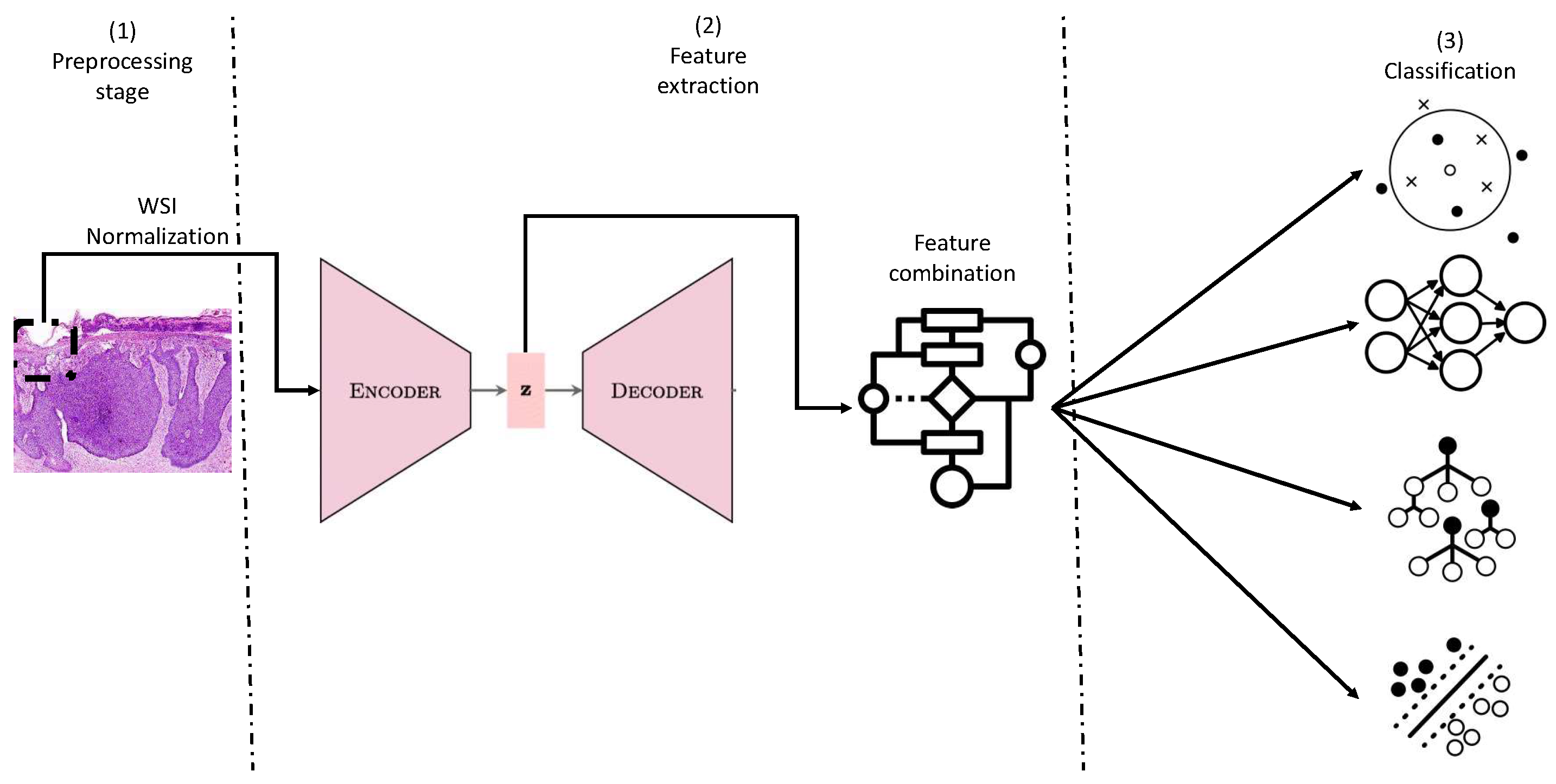
Figure 2.
Autoencoder for feature extraction.
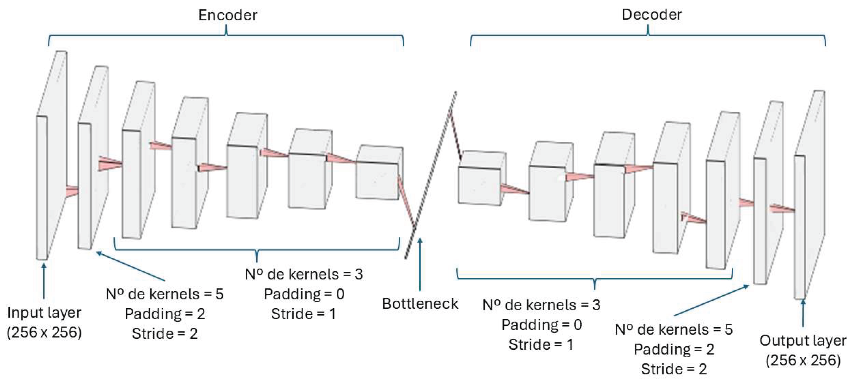
Table 7.
Accuracies for the four approaches.
| Approach | Training accuracy | Validation accuracy | Test accuracy |
| KNN | 100.00% ± 0.00 | N/A | 97.95% |
| SVM | 84.96% ± 0.00 | N/A | 75.00% |
| MLP | 90.17% ± 6.00 | 85.69% ± 14.40 | 76.53% |
| Random Forest | 100.00% ± 0.00 | N/A | 97.95% |
Table 8.
Specificity and sensitivity for the best approach.
| Stage | Training Specificity | Test Specificity | Training Sensitivity | Test Sensitivity |
| KNN Model | 100.00% ± 0.00 | 95.55% | 100.00% ± 0.00 | 100.00% |
| RF Model | 100.00% ± 0.00 | 97.77% | 100.00% ± 0.00 | 100.00% |
Table 9.
Comparison with baseline.
| Model | Test accuracy |
| Our model | 97.95 % |
| EfficientNetB3 | 85.71 % |
| DenseNet121 | 95.24% |
| ResNet50V2 | 84.13 % |
Table 10.
Physicians’ evaluation.
| Case | Asymmetry | Atypia | Maturation | Pegatoid extension | Mitosis | Pigment |
| Pigmented lentiginous nevus FP | 0 | 2 | NA | 0 | 0 | 3 |
| Deep blue nevus FP | 3 | 0 | 2 | 0 | 0 | 3 |
Disclaimer/Publisher’s Note: The statements, opinions and data contained in all publications are solely those of the individual author(s) and contributor(s) and not of MDPI and/or the editor(s). MDPI and/or the editor(s) disclaim responsibility for any injury to people or property resulting from any ideas, methods, instructions or products referred to in the content. |
© 2025 by the authors. Licensee MDPI, Basel, Switzerland. This article is an open access article distributed under the terms and conditions of the Creative Commons Attribution (CC BY) license (http://creativecommons.org/licenses/by/4.0/).
Copyright: This open access article is published under a Creative Commons CC BY 4.0 license, which permit the free download, distribution, and reuse, provided that the author and preprint are cited in any reuse.


