Submitted:
30 May 2025
Posted:
03 June 2025
You are already at the latest version
Abstract
Studying the vertical and horizontal distribution of particulate matter at the hectometer scale in the atmosphere is essential for understanding its sources, transportation, transmission and its impact on human health. In this study, we developed a method based on hyperspectral equipment to rapidly obtain the three-dimensional distribution of aerosol extinction by using multiple azimuths, optimizing the selection of elevation angles, and reducing the acquisition time for individual spectra. This method employed observations from different azimuth angles to represent particulate matter concentrations in various directions. The correlation coefficient between the hyperspectral observations and in-situ measurement was 0.627. The observational results indicated that the aerosol extinction (AE) profile followed an exponential distribution, with the majority of the aerosol located below 1 km in height. The vertical distribution suggested that the particulate matter originates from local near-surface emissions. The horizontal distribution indicated that the northeastern urban areas and the eastern rural areas were the primary regions with high concentrations of particulate matter. From the observation results, we speculate that overpass construction and rural heating and cooking wood burning are two potential sources of emissions, respectively. Forward trajectory analysis revealed that, under the complex terrain of the Guanzhong Plain, particulate matter locally emitted during the observation period was likely transported primarily to the western urban area of Xi'an, the northern region of Qingyang, and the southwestern area of Shangluo. Moreover, health risk obtained using the exposure-response function model indicated that even within the same town, differences of particulate matter concentration and population density could lead to varying health exposure risks. For instance, in the 200° and 210° directions, which represent adjacent urban areas less than 1 km apart, the number of PM2.5-related illness cases in the 210° direction was 20.83% higher than that in the 200° direction.
Keywords:
hyperspectral
; aerosol
; three-dimensional spatial distribution
; emission source identification
; health risk assessment
1. Introduction
Air pollution, especially aerosol pollution, poses significant health risks to humans [1]. Fine particulate matter in aerosols can penetrate the alveoli and enter the bloodstream, contributing to various diseases, including respiratory and cardiovascular disorders [2,3,4,5]. According to relevant research in India, over a three-year period since 1992, premature deaths due to exposure to particulate matter increased by 28% [6]. The Health Effects Institute (HEI) reported that air pollution is the third leading risk factor for mortality in South and Southeast Asia, with particulate matter being a major contributor to the disease burden [7].
Investigating the spatial distribution of particulate matter at a hundred-meter resolution is crucial for emission source identification, pollution control, transport analysis, and risk assessment. In urban areas, primary emissions of particulate matter from vehicular exhaust, industrial discharges, and dust generated at construction sites constitute a significant source of PM2.5 [8]. The scale of those particulate matter emission sources in urban areas is typically in the order of hundreds of meters. Urban and rural areas are typically exposed to different types and concentrations of particulate matter due to various factors, such as solid fuel combustion and dust from construction sites [9,10]. Rakefet Shafran-Nathan et al. employed a distributed sensor network to observe particulate matter concentrations at fine spatial scales, revealing significant spatial variability at the neighborhood level, which was closely associated with human activities such as traffic and residential behaviors [11]. Therefore, it is essential to obtain data at a hundred-meter resolution to conduct source apportionment analysis, identify high-emission zones, and implement targeted regional intervention measures accordingly. Zhao Y. Z. et al. used hundred-meter-scale data to track the real-time emission sources of ambient VOCs, particulate matter, and O3 and found that pollution sources were mainly concentrated at traffic intersections, industrial emissions, and residential areas [12]. The spatial resolution of particulate matter concentration and population density exerts a significant impact on the assessment of health effects related to particulate matter [13]. Heming Bai et al. aggregated satellite-derived PM2.5 concentration and population data at a 1 km resolution in China to coarser resolutions to evaluate the impact of resolution on health assessments. They found that as the resolution decreased, the national population-weighted mean (PWM) PM2.5 concentration declined, indicating that lower resolution data would underestimate health risks. [14]. Therefore, obtaining high-resolution particulate matter distribution at the hectometer scale allows for a more accurate assessment of air quality impacts on different regions and populations, helping policymakers develop more effective health protection measures. However, there is still a lack of comprehensive three-dimensional monitoring that simultaneously captures both the horizontal and vertical distribution of aerosols.
In recent years, with the advancement of technology, observation methods have become increasingly diverse. Commonly used methods include in-situ observations, satellite remote sensing, and ground-based remote sensing. In-situ observations refer to methods that directly sample and measure particle concentrations in the atmosphere. These methods typically include filter-based methods [15,16], light scattering methods [17], and charge methods [18]. In-situ observation methods are typically installed at meteorological stations, monitoring sites, or mobile platforms and are widely used in urban air quality monitoring. However, in-situ observations have the drawback of limited spatial coverage. Particle monitoring instruments can be mounted on various platforms, such as balloons [19,20], aircraft [21,22], drones [23,24,25], and vehicles [26]. However, their coverage remains limited due to factors such as high costs.
Satellite remote sensing mainly relies on satellite sensors to measure reflected light from the atmosphere and surface. By analyzing the reflection spectra at different wavelengths, aerosol optical depth (AOD) and other information can be retrieved [27,28]. Tingting Liao et al. used the CAPLISO level-2 nighttime aerosol profile product to detect the seasonal distribution and vertical structure of four types of aerosols in the southwestern region [29].Chen Q. X. et al. analyzed the spatiotemporal distribution characteristics of major aerosol types over China using MODIS satellite data from 2008 to 2017 [30].Zhang T. et al. estimated PM2.5 concentrations in several regions of China, including the Beijing-Tianjin-Hebei region and the Yangtze River Delta, based on AOD data from Himawari-8 [31].Although satellite remote sensing can achieve long-term and wide-area aerosol monitoring, it is difficult to simultaneously address both vertical and horizontal measurements, and its spatial resolution is low, making it challenging to support source apportionment tasks.
Ground-based remote sensing mainly detects optical properties of aerosols through the scattering, absorption, and other interactions between light and aerosol particles in the atmosphere. Common instruments include sun photometers, LIDAR and MAX-DOAS. Sun photometers mainly use the phenomenon of solar radiation being scattered and absorbed as it passes through the atmosphere. Zheng Y. et al. investigated the optical properties of aerosols in Beijing from 2013 to 2018 using sun photometer observation data. [32]. However, the results obtained from sun photometers represent the total column distribution, lacking vertical distribution information, and their coverage is limited. LIDAR detects the vertical distribution of aerosols by emitting laser pulses and receiving the backscattered echo signals from aerosol particles [33,34]. Zhizhong Sheng et al. used LIDAR and sun photometers to study the vertical distribution and optical properties of sand dust, haze, and aerosols in the Beijing area in 2017 [35]. Tianze Sun et al. used observation data from LIDAR and sun photometers to study the monthly variation of aerosol vertical structure in the Yangtze River Delta region [36]. Although LIDAR can observe aerosols either horizontally or vertically, it is difficult to perform both vertical and horizontal observations simultaneously.
MAX-DOAS is a hyperspectral method based on differential optical absorption spectroscopy (DOAS) used to measure aerosol optical properties. It is widely applied to observe aerosol spatial distribution and track pollution sources. Xiaomei Li et al. used MAX-DOAS instruments to study the vertical distribution and potential sources of aerosols in the Fenwei Plain [37]. However, in previous studies, MAX-DOAS instruments have typically been used for vertical observations of particulate matter [38] and horizontal distribution of trace gases. Chuan Lu et al. used hyperspectral to obtain high spatiotemporal resolution horizontal distribution results for NO2. However, there are few studies that use MAX-DOAS to simultaneously observe both the horizontal and vertical distributions of aerosol extinction coefficients [39].
This study proposed a method based on hyperspectral technology to efficiently obtain aerosol extinction profiles by using different azimuth angles and optimizing the elevation angle sequence and single-spectrum acquisition time. Based on these results, we analyzed the three-dimensional spatial distribution characteristics of aerosols and traced the primary emissions of particulate matter. Finally, we conducted a detailed health risk assessment within the city. The findings provide novel insights for air pollution control and public health risk assessment.
2. Methods
2.1 Overall Observation Scheme Design
Figure 1 below shows the technical flowchart of our work. Firstly, during the design of the spectral observation plan, we chose a two-dimensional hyperspectral device and collected spectra from different azimuths by rotating the telescope with a motor. At the same time, we optimized the elevation angle sequence and the spectral acquisition time to adapt to the observations in the Gaoling District of Xi’an, balancing between acquisition rate and quality. After collecting the spectra, we used QDOAS for spectral fitting to obtain dSCD (Differential Slant Column Density). Next, we applied the OEM algorithm and the SCIATRAN radiative transfer model to invert the dSCD, which provided the aerosol extinction profiles corresponding to each spectrum. By combining the results from different azimuths, we obtained a three-dimensional aerosol extinction distribution. We then assessed the PM2.5 health exposure risks within the observation range using a traditional linear model and exposure-response functions. Furthermore, we evaluated the particle propagation impacts using the Meteoinfo and HYSPLIT models. The observation site and relevant experimental methods used in this study are described in Section 2.2, Section 2.3, Section 2.4, Section 2.5 and Section 2.6.
2.2 Observation Site
The hyperspectral equipment system was mounted on the rooftop of Aoyun Huafu Community in Gaoling District, Xi’an City, at an altitude of approximately 70 meters, with the longitude and latitude being 109.1034°E and 34.5269°N respectively. This study specifically focused on the sources of particulate matter during the autumn and winter seasons, as pollution levels are typically more severe during this period, posing greater health risks. Therefore, observations were conducted during these seasons. There were no taller buildings in the vicinity, and the field of vision was unobstructed. The observation period ranged from September 16, 2020 to November 22, 2020. The schematic diagram of the observation is depicted in Figure 2. In the observation schematic diagram, the green part represents the vegetated surface, and the vegetation types might include urban green plants and farmland crops, while the yellow part represents bare soil. The northeastern and southwestern directions of the observation point have large areas of bare soil and are urban areas with a relatively high population density. The eastern area is mostly covered by vegetation and is a rural area with a relatively low population density.
The concentrations of PM2.5 during the research period were derived from the China National Environmental Monitoring Centre (CNEMC), and the selected data were the hourly average values of PM2.5 at the monitoring station in the Economic Development Zone. The geographical coordinates of the station are 108.9459°E, 34.3521°N.
2.3 Instruments and Inversion Approaches
The hyperspectral instrument adopted in this study is of the model Airyx Skyspec-2D (Airyx SkySpec, Airyx, Heidelberg, Germany, https://www.airyx.de/, accessed on September 16, 2020). This instrument primarily comprises three components: a stepping motor, a telescope, and a spectrometer. The telescope employs quartz lenses with an ultraviolet light antireflection film coated on the surface and is installed on a two-dimensional rotating stepping motor via a bracket. It is capable of conducting 360° horizontal and 0 - 90° vertical rotational scans, with a field of view of 0.2° * 0.8°. The telescope and the stepping motor must be installed outdoors. The stepping motor drives the telescope to collect solar scattered light from various directions and elevations, and the received light beam is conducted to the spectrometer unit through a quartz optical fiber. Within the spectrometer unit, there are three subunits: the Vis visible light spectrometer, the UV ultraviolet light spectrometer, and the temperature control system. The light beam is split into two beams by the optical fiber beam splitter and enters the Vis/UV spectrometers respectively. The temperature control system ensures that the spectrometer unit remains in a constant temperature state, stabilizing its temperature at 20 ± 0.05°C, so as to reduce the dark current and enhance the signal-to-noise ratio.
In order to acquire vertical profiles promptly, in contrast to the traditional elevation sequence configuration (the traditional elevation sequence is set as 1°, 2°, 3°, 4°, 5°, 6°, 8°, 10°, 15°, 30°, 90°) [40], in this research, the elevation sequence was set as 3°, 5°, 8°, 10°, 30°, and 90°, while the azimuth angle was set from 30° to 210° with an interval of 10°, totaling 19 azimuths. The acquisition time for a single spectrum was 20 seconds. Since the fitting was for O4 and the absorption intensity of O4 is greater than that of other trace gases such as HCHO, and its concentration is relatively high, a 20-second acquisition time is adequate for the signal-to-noise ratio. Since we used a two-dimensional hyperspectral instrument, the telescope could scan in multiple directions by rotating the motor, enabling the acquisition of aerosol extinction profiles across different azimuthal angles. We optimized the elevation angle sequence and single-spectrum acquisition time, achieving an optimal balance between temporal efficiency and data quality. This approach allowed us to quickly obtain high-quality aerosol extinction profiles from various directions. After optimizing the elevation angle sequence and the integration time of each spectrum, it took approximately 45 minutes to complete a full azimuthal scanning cycle. In contrast, the traditional configuration requires about 4 hours to complete the same process. The conventional setup is therefore unable to retrieve extinction profiles within a short time frame. Due to the extended duration, significant variations in boundary layer height (BLH) can occur within a single azimuthal sequence. For example, if the azimuthal scanning sequence spans from 8:00 a.m. to 12:00 p.m., the increase in boundary layer height (BLH) around noon may lead to a significant discrepancy in BLH between the profiles obtained at the beginning and those at the end of the sequence.
In this study, we used RMS to evaluate the spectral fitting quality and the Degrees of Freedom (DOF) to assess the quality of the retrieved vertical profiles. A complete measurement sequence consists of 19 azimuth angles and the corresponding elevation sequences for each azimuth angle, and each complete measurement sequence lasts approximately 40 minutes. The intensity of scattered sunlight determines the exposure time and the number of scans, and is automatically controlled through a script. Scattered sunlight is automatically collected during the day, while dark current and offset spectra are automatically collected at night and subtracted from the spectra collected during the day. To avoid severe stratospheric absorption effects, only spectra with a solar zenith angle (SZA) greater than 75° are collected.

Table 1.
Instrument observation time, elevation and azimuth setting.
| Date | mode | Azimuth angle | Elevation |
| From September 22, 2020, to November 22, 2020. | hybrid | 30˚-210°(interval=10°) | 3˚, 5˚, 8˚, 10˚, 30˚, 90˚ |
2.4 Spectral Analysis And Inversion of Aerosol Extinction Profile
In this study, the QDOAS software (http://uv-vis.aeronomie.be) developed by the Royal Belgian Institute for Space Aeronomy (BIRA-IASB) was utilized to achieve the inversion of the differential slant column concentration of O4. The zenith spectra in each elevation sequence were adopted as reference spectra for DOAS fitting. The range of 338 - 370 nm was selected for the fitting of O4 in this study. Referring to the recommended settings of the CINDI-2 comparison campaign, the absorption cross-sections of trace gases [41] were applied during the inversion process.
For the DOAS fitting results, those with RMS > 2.0×10⁻³ were eliminated. According to relevant studies, the RMS threshold for O4 fitting is typically set at 2 × 10⁻³. An RMS value below this threshold is generally considered acceptable for a reliable spectral fit [42]. After elimination, the retention rate of O4 was: 91.39%. The QDOAS configuration is presented in the following table.
Table 2.
QDOAS fitting configuration.
| Parameter | Data Source | O4 |
| Wavelength range | 338-370 | |
| NO2 | 298 K, I0 correction(SCD of 1017 molecules cm-2) [43] | √ |
| NO2 | 220 K, I0 correction(SCD of 1017 molecules cm-2) [43] | √ |
| O3 | 223 K, I0 correction(SCD of 1020 molecules cm-2) [44] | √ |
| O3 | 24 K, I0 correction(SCD of 1020 molecules cm-2) [44] | √ |
| O4 | 293K [45] | √ |
| BrO | 223K [46] | √ |
| H2O | 296K,HITEMP [47] | √ |
| HCHO | 297K [48] | √ |
| Ring | Calculated with DOAS [49] | √ |
| Wavelength calibration | A high-resolution solar reference spectrum (SAO2010 solar spectra) [50] | √ |
| Polynomial degree | Order3 | |
| Intensity offset | Constant |
Figure 3 below shows an example of QDOAS fitting results; additional examples are provided in the supplementary materials. Moreover, the corresponding data table has been uploaded to Zenodo for public access. The link to the page has been placed in the Data Availability section.
The average RMS obtained from DOAS fitting of the collected spectra was 0.0011. With over 90,000 spectra acquired in this study, a retention rate of 91.39% was achieved after filtering out fitting results with an RMS greater than 2 × 10⁻³. Therefore, the spectral data used in our fitting process are considered reliable.
The vertical aerosol profile is retrieved from the differential slant column concentrations measured by MAX-DOAS through the optimal estimation method (OEM) [51]. In this study, we used the SCIATRAN forward radiative transfer model, which is widely applied in the retrieval of vertical profiles from MAX-DOAS measurements [52].
The core of the optimal estimation algorithm is the introduction of the cost function . The result of minimizing the cost function by constantly adjusting the value of the posterior state vector is the optimal solution of the state vector . The specific expression of the cost function is as follows:
In the equation, is the a priori state vector, and and respectively represent the measurement covariance and the a priori covariance matrices. The aerosol extinction profile can be directly inverted using parameters such as the DSCDs results of O4 and the a priori aerosol profile.
The principal parameters in the optimal estimation algorithm encompass the gain function G, the average kernel matrix (Average Kernel, AVK), and the degrees of freedom, among others. The average kernel matrix A reflects the sensitivity of the genuine state vector to the inversion result . The specific meaning of the element a_ij in matrix A is the sensitivity of the real atmosphere at layer i to the inversion result at layer j. The closer the diagonal element is to 1.0, the higher the credibility of the inversion result of the corresponding layer.
The trace of the average kernel matrix represents the Degrees of Freedom of the signal. The DOF indicates the number of independent pieces of information provided by the state vector. Ideally, the DOF should be equal to the dimensionality of the state vector. Before data analysis, the DOF magnitude is commonly used as a criterion for assessing the inversion quality, filtering out contour results with substandard quality and low confidence.
In the inversion process, the atmosphere is divided into 19 layers from 0 to 4 km, with the lowest layer at 0.04 km and the highest at 3.84 km, and a vertical resolution of 0.2 km. An exponential decay prior method with a height of 1 km is used to invert the aerosol profile. The prior extinction profile is set as an exponential function, with a ground-level extinction coefficient of 0.3 km-1, a scale height of 1 km, a prior uncertainty of 100%, and a correlation height of 0.5 km. Additionally, we adopted the following fixed aerosol optical properties: a surface albedo of 0.05 and an asymmetry factor of 0.72. The central wavelength used was 360.8 nm. The SCIATRAN model also utilized fixed profiles of temperature, pressure, and atmospheric constituents, with different profiles applied for varying times and geographic locations. Additionally, the absorption cross-section of O4 was included in the simulation. This work also inverts the single scattering albedo (SSA). The retrieval of single scattering albedo from hyperspectral observations was based on the differential slant column density data obtained from QDOAS spectral fitting. The SCIATRAN radiative transfer model was employed, and the optimal estimation method was used to iteratively compare the simulated and observed data, allowing for the final retrieval of SSA.
2.5 Cluster Analysis
This study analyzes the forward trajectories of the Gaoling District in Xi’an using the TrajStat plugin in the Meteoinfo software developed by the team of Yaqiang Wang (http://www.meteothink.org/), and performs clustering analysis using the HYSPLIT model. The HYSPLIT model is a system developed jointly by the National Oceanic and Atmospheric Administration (NOAA) and the Australian Bureau of Meteorology for computing and analyzing the sources, transport, and diffusion trajectories of atmospheric pollutants. The data used in this study are from the Global Data Assimilation System (GDAS) provided by the National Centers for Environmental Prediction (NCEP) (ftp://arlftp.arlhq.noaa.gov/pub/archives/gdas1/, accessed on 20 December 2024) [53].
Therefore, this method has certain limitations in our study. Due to the lack of high-resolution meteorological data within the observation area, we were only able to assess regional-scale pollutant transport rather than conduct a refined analysis of intra-urban transportation.
2.6 Health Effect Assessment
This study uses an epidemiology-based exposure-response function to assess the health risks of particulate pollution within the monitoring range of the Gaoling District site in Xi’an. The exposure-response function links changes in air quality with human health effects and is a crucial method for quantitatively assessing the health impacts of air pollution. The exposure-response function is widely used in many epidemiological studies to estimate health effects related to air pollution. This model is designed for short-term exposure risk assessment. For instance, Haidong Kan et al. applied this method to evaluate the health risks of atmospheric particulate pollution in Shanghai. [54]. Given a specified concentration, the following equation can be used to calculate the number of cases directly associated with PM2.5 pollution:
In the equation, C represents the actual PM2.5 concentration (µg/m3). represents the reference baseline PM2.5 concentration (this study adopts the WHO standard: 25 µg/m3); is the exposure-response coefficient (Details are provided in Table S1), is the population health risk at , is the population in the study area, and E is the number of cases directly related to the current PM2.5 concentration.
In this study, a traditional linear model is used to convert the aerosol extinction coefficient into PM2.5 concentration [55]. In the conventional linear model, aerosol extinction and total particulate mass concentration exhibit a linear relationship, which can be expressed by the following conversion formula:
Where, is the mass concentration of PM2.5, is the aerosol extinction coefficient.
3. Results and Discussion
3.1 Result Verification
The method used in this study to validate the accuracy of the MAX-DOAS inversion results follows Qianqian Hong et al. [56]. The aerosol extinction coefficient (AE) at the lower layers obtained by MAX-DOAS is compared with CNEMC data, as shown in Figure 4. Prior to the correlation analysis, the data were partially processed. The aerosol extinction profile at the lower layers and the PM2.5 concentration at CNEMC sites were selected for analysis, and the following quality control measures were applied to the AE: 1. Data collected on clear weather days were selected to ensure spectral quality (Cloud-contaminated data were excluded from the analysis.); 2. Profiles with Degrees of Freedom within the range of 2-4 and Chi-squared values less than 200 were selected to ensure the quality of the profiles. 3. Instrument results were converted to hourly averages. The correlation coefficient obtained in this study was 0.627. Shanshan Wang et al. compared hourly data from MAX-DOAS with in-situ observations in Madrid, Spain, and found a correlation of 0.6385 [57]. In addition to the commonly used linear correlation analysis method, we also applied Spearman’s rank correlation analysis to examine the correlation between MAX-DOAS and CNEMC data. This analysis yielded a correlation coefficient of 0.638. This indicates that the data from the hyperspectral site inversion in this study are reliable.
In similar studies, Dimitris Karagkiozidis et al. used a traditional zenith angle sequence, achieving a Degree of Freedom of 2.17 in the aerosol vertical extinction profile inversion [58]. Wang Yang et al. used zenith angle sequences of 5°, 10°, 20°, 30°, and 90° to invert the aerosol profile in Wuxi, China, with a DOF of 1.5 [59]. In this study, the zenith angle sequence used for inverting the aerosol extinction profile resulted in a DOF of 1.826, indicating that the profile quality remained good even after reducing the angle sequence. Based on this, the spatial distribution of particulate matter and its health impacts are analyzed.
3.2 Spatial and Temporal Distribution Characteristics
3.2.1 Overall Distribution
As shown in Figure 5, panel (a) and panel (b) represent the overall average horizontal and vertical distribution results during the observation period, respectively. In panel (a), a sector is used to represent the observation range for convenience. Each sector unit corresponds to the average extinction profile results at the lower layers for a given azimuth angle, with the radius of the sector representing an actual distance of 5 km, as the average effective optical path during the observation period is approximately 5 km. Panel (b) represents the average aerosol extinction profile at a height of 4 km. Given that it corresponds to profiles at different azimuth angles, an arcuate representation is used in panel (b).
During the observation period, it was found that the horizontal distribution of the aerosol extinction coefficient generally shows higher values in the northeast and lower values in the southwest. The AE is maximum at a 30° azimuth in the northeast, reaching 0.871 km-1, and gradually decreases towards the southwest, with the lowest value at a 190° azimuth, where AE is 0.624 km-1. In the northeast direction, the area is primarily urban, featuring a large interchange under construction, which generates significant dust. We speculate that this may be the reason for the elevated particulate matter concentration in this direction. To the east of the observation site, the area is predominantly rural, where firewood is still widely used for heating and cooking. This process releases a substantial amount of particulate matter, likely contributing to the higher AE values in this direction. The aerosol concentration follows an exponential distribution in the vertical direction, primarily concentrated below 1 km, with the average AE peak occurring at 200 m. The AE is also highest at the 30° azimuth, reaching 0.974 km-1. The results suggest that there may be near-surface emissions and generation of particulate matter in the northeast direction.
In this study, within a similar time period, the boundary layer height was considered to be uniform within this small range. The spatial distribution of aerosol extinction coefficients revealed distinct variations in concentrations despite the relatively uniform boundary layer height (BLH) distribution during similar time intervals. T The aerosol extinction exhibits uneven vertical distribution, showing a distinct exponential (e) distribution. These findings suggest the presence of potential emission sources near the surface.
Figure 6 shows the time variation of the vertical distribution at 30°, 100°, and 200° during the observation period. These vertical distribution results represent the average over the observation period and show the overall distribution during this time. The results indicate that the aerosol extinction profile follows an exponential distribution. In the 30° direction, the AE values are consistently high throughout the day, with the overall distribution primarily below 1 km. In the morning, the average peak is at 200 m, with a maximum AE of 1.355 km-1. As time progresses, the boundary layer rises, and pollutants gradually disperse into higher altitudes. At midday, the aerosol reaches altitudes around 1 km, with the average peak at 400 m and a maximum AE of 1.247 km-1. By the afternoon, the aerosol descends back below 1 km, with the average peak at 200 m and a maximum of 1.135 km-1. The persistently high AE values observed throughout the day in this direction may be attributed to dust emissions caused by construction activities and traffic-related transportation.
The 100° direction represents the vertical profile of a rural area, where the profile shows higher values in the morning and evening, with pollutant heights primarily below 1 km. The average peak is at 200 m, with the highest AE reaching 1.833 km-1. During the midday period, the dissipation of pollutants typically leads to a reduction in particulate matter concentrations. However, under conditions of elevated boundary layer height, a relatively high aerosol extinction value of approximately 0.816 km−1 was still observed near the surface, higher than that in the urban area. The midday peak may be attributed to particulate emissions from the combustion of firewood used for cooking in rural areas.
In the 200° direction, the observation area is primarily urban. Pollutants in this direction are mainly distributed in the morning and evening, with heights primarily below 800 m. The average peak is at 200 m, with the highest AE values in the morning and evening reaching 1.189 km-1 and 1.303 km-1, respectively. This distribution is likely due to photochemical pollution in the morning, which accumulates a large amount of pollutant, dissipates around midday, and then begins to accumulate again in the evening. The maximum AE value in rural areas is approximately 37.9% higher than in urban areas. This may be because urban areas have fewer combustion emissions (such as wood burning), leading to lower particulate matter concentrations in the midday period compared to rural areas.
In aerosols, a higher black carbon (BC) content typically results in a lower single scattering albedo (SSA). Xiaolin Zhang et al. demonstrated that BC exhibits stronger light-absorbing properties than dust particles, and this enhanced absorption leads to a decrease in SSA compared to dust-dominated aerosols [60]. According to Tamar Moise et al., the SSA of pure black carbon can approach 0 under ideal conditions, while SSA for mixed BC aerosols ranges between 0.2 and 0.9, and that of organic aerosols lies between 0.83 and 0.95 [61]. Similarly, M. Hess et al. found that the SSA of non-BC aerosols in clean continental regions is approximately 0.972, whereas the SSA in urban areas with higher BC concentrations is about 0.817. For mineral dust aerosols, the SSA is around 0.888 [62]. In our work, the mean SSA of the aerosol in the northeast direction is 0.748, and the mean SSA of the aerosol in the east direction is 0.712. It may be that the higher black carbon content in rural areas in the east and the higher dust content in aerosols in the northeast lead to a relatively lower SSA in eastern aerosols. After obtaining above results, we visited the overpass junction and the villages at the foot of the mountain, and found that the overpass was under construction, and most of the villages at the foot of the mountain still burned wood and coal for heating and cooking. Since biomass burning is one of the important sources of black carbon, we combined the SSA obtained by inversion and the field visit, we guessed that the overpass intersection under construction and the rural biomass burning are two potential emission sources.
Qili Dai et al. studied the chemical composition of PM2.5 in Xi’an and found that residential heating and coal-based cooking are significant primary emission sources [63]. Research by Song Y. Z. et al. indicates that PM2.5 concentrations in Xi’an’s urban areas are primarily from local emissions, with major contributions from industry, transportation, household activities, and dust. These findings are consistent with the analysis in this study [64].
3.2.2 short Time Change
The following results represent a typical case with characteristic features. Figure 7a and Figure 7b show the horizontal distribution of AE and the vertical distribution at different azimuths for the period between 7 and 8 AM on September 25, 2020. The horizontal distribution shows higher values in the northeast and east directions, lower values in the southwest, and higher values in rural areas compared to urban areas, which is consistent with the average results. The highest AE value is at the 160° azimuth, reaching 1.617 km-1. The aerosol extinction profile follows an exponential distribution, with pollutants mainly concentrated below 800 m. The average peak is at 200 m, and the maximum AE reaches 1.627 km-1. Figure 7c is a satellite image of the overpass area, which has sparse vegetation and ongoing construction. The presence of sand and gravel particles makes it easy for vehicles to stir up dust, leading to pollution. Figure 7d is a photo of the observation point, showing fewer particles in the nearby urban area and more particles near the village at the foot of the mountain. The particulate matter concentration decreases with height, following an exponential distribution, which is consistent with the observed results. We speculate that this spatiotemporal distribution is most likely caused by the two potential emission sources mentioned above.
Figure 8 shows the horizontal and vertical distribution results around 3 PM and 5-6 PM. The horizontal distribution in Figure 8a shows that the particulate matter concentration near the surface in the afternoon is generally lower, with significantly higher concentrations in the northeast direction compared to other directions. The vertical distribution in Figure 8b shows that in the afternoon, pollutants are primarily concentrated below 1 km. Due to the dissipation of pollutants and the elevation of the boundary layer, the particulate matter concentration is lower during this period.
The results in Figure 8c show that in the evening, the concentration of particulate matter near the surface is high across the observation range, with the highest value reaching 1.975 km-1. The concentration of particulate matter in the rural areas in the 70°-130° azimuth range to the east is relatively lower. The vertical distribution in Figure 8d shows that in the evening, particulate matter is primarily concentrated below 800 m, with the peak value at 200 m and the highest AE reaching 1.938 km-1. This high value may be due to the lowering of the boundary layer, which causes pollutants to accumulate again, resulting in a high aerosol extinction coefficient.
Based on in-situ observation data, monthly and seasonal variations in Xi’an’s Gaoling District were obtained. Detailed results and conclusions can be found in Figure S2 in the supplementary materials.
The Gaoling District of Xi’an is located in the Guanzhong Plain, which is bordered by the Qinling Mountains to the south and the northern Shaanxi Plateau to the north, resulting in a complex topography. To assess the impact of regional transport on atmospheric pollutants in complex terrain, forward trajectories at 40m, 200m, 400m, and 800m heights in Gaoling District of Xi’an were calculated for the period from September to November 2020. The particle lifetime was considered, and 24-hour air mass back-trajectories were used for the analysis. Figure 9 shows the key clusters of potential transport at 40m, 200m, 400m, and 600m heights in Gaoling District of Xi’an. For air masses at 40m, 200m, and 400m, each height has three transport paths. One is a short-distance transport path: the short-distance transport at 40m and 400m is mainly toward the western part of Xi’an, accounting for 46.72% and 49.81%, respectively, while at 200m, the transport is mainly toward the southern part of Xi’an, accounting for 49.94%. Cluster 2 at 40m, and Cluster 3 at 200m and 400m, mainly transport toward the northern part of Shangluo and the Hunan region. Cluster 3 at 40m primarily follows the route from Binzhou to Qingyang. As the height increases, the transport trajectory in this direction gradually approaches Tongchuan. When the air masses transport westward along the northern part of the Guanzhong Plain, the relatively low elevation of the Binzhou area allows the air masses to follow this lower-altitude transport route. At 800m, there are four main transport trajectories. Cluster 1 has a shorter path, starting from Gaoling District, moving to the western part of Xi’an, and then to Yongshou County in Xianyang, accounting for 33.02%. Cluster 2 transports northward along the western part of Tongchuan, accounting for 22.60%. Cluster 3 moves southward along Shangluo toward Hunan, accounting for 27.53%. Cluster 4 transports northeastward along Tongchuan, reaching the northwest of Linyi, accounting for 16.85%. Since Gaoling District of Xi’an is located in the heart of the Guanzhong Plain, and northeastern winds prevail in Xi’an throughout the year, air masses have a high probability of passing through Xi’an and transporting toward the western part of the Guanzhong Plain. Due to the elevation difference of over 800m between Gaoling and northern areas like Tongchuan, only air masses from higher altitudes will transport toward the northeast. However, as the vertical results show that particulate matter in Gaoling is distributed below 1 km, the amount of particulate matter transported toward the northeast is relatively low.
Figure 10 shows the forward trajectories at 40m, 200m, 400m, and 800m on September 25. It can be observed that at all four heights, there are only two long-distance transport paths. The two transport paths at 40m, 200m, and 400m all follow the route from Binzhou to Qingyang. At 800m, Cluster 1 moves northward along Chunsan County and the western part of Qingyang, while Cluster 2 moves northward along the western part of Tongchuan. On that day, the transport paths primarily moved toward the northwest of Gaoling District, which coincides with the direction of the highest population density in Gaoling. This area should be a focus for particulate matter exposure risks.
3.3 Health Impact
The health risks associated with PM2.5 are closely linked to public health and are receiving increasing attention. In this study, the population within a 5 km radius of the site in all directions was selected as the research area for health risk assessment. Health assessments were conducted based on the average PM2.5 from the hyperspectral instrument, with Table S1 listing the incidence rates and PM2.5 exposure-response coefficients for selected health outcomes. The atmospheric conditions within the observation range are poor, indicating a polluted urban environment. The number of cases potentially associated with particulate air pollution within the observation range was calculated using the exposure-response function, result frequency, exposure concentration, and threshold levels, as shown in Table 3. Figure 11 presents the distribution map of cases for overall diseases as well as for selected individual diseases. Additional disease case distribution maps can be found in the supplementary materials.
Particulate air pollution may result in 54 deaths, 585 asthma attacks, 71 cases of chronic bronchitis, 2,652 cases of acute bronchitis, 27 hospitalizations for cardiovascular diseases, 16 hospitalizations for respiratory diseases, along with 1,022 cases of internal medicine visits and 108 pediatric consultations. Additionally, there are 41,678 cases of restricted activity. The total number of individuals exposed is 4,429, accounting for 11.06% of the total population. Compared to cities with good air quality, the health risks of particulate matter in Gaoling District are relatively high, and strict control of particulate emissions should be implemented.
The results show that although biomass burning leads to higher particulate concentrations in rural areas, the lower population density in these areas results in a smaller health impact from particulate matter. In urban areas, both high and low concentrations of particulate matter have a significant impact on human health. For example, the northeast direction has higher particulate concentrations, while the southwest direction, with its higher population density, also shows a higher number of potential cases. Even within the same town, differences in concentration and population density can lead to varying health impacts. For instance, at the 200° and 210° directions, which represent adjacent urban areas less than 1 km apart, the number of PM2.5-related cases in the 210° direction is 20.83% higher than in the 200° direction.
4. Conclusions
This study proposed a novel method based on hyperspectral instruments to simultaneously obtain the vertical and horizontal distributions of aerosol extinction coefficients at different azimuth angles by optimizing the elevation angle sequence and the acquisition time of individual spectra. The correlation coefficient between the hyperspectral observations and CNEMC station data was 0.627. The degree of freedom during the profile inversion was 1.826. The aerosol extinction profile followed an exponential distribution, with the majority of aerosol concentration located below 1 km in height. The particle concentration in the northeastern urban area remained high throughout the day, while high concentrations in the southwestern and eastern areas were mainly concentrated in the morning and evening. At noon, with the boundary layer rising, particulate matter dispersed, and concentrations decreased. The midday particulate concentration in the eastern rural area was higher than in the southwestern urban area. The exponential vertical distribution results indicated that particulate matter likely originates mainly from local near-surface emissions. Combined with the observation results, the SSA of inversion and the field visit, we conclude that there may be two potential emission sources within the observation range, namely the overpass under construction and the biomass burning in the countryside. Based on the horizontal distribution, two potential emission sources were identified: one being a construction site for a highway interchange, where dust from construction and traffic may have contributed to particulate pollution. The other source was the rural area, where burning firewood for heating and cooking emitted large amounts of particulate matter. Based on the above results, the study examined the impact of local emissions from the Gao Ling District of Xi’an on regional transport in complex terrain and its effects on nearby cities. Using forward trajectory analysis, four main transport paths for particulate matter in complex terrain were identified: Gao Ling District to the western and southern urban areas of Xi’an, Gao Ling to the Binzhou-Qingyang direction, Gao Ling to the northwest of Tongchuan and Linfen, and Gao Ling to Shangluo. The path that transported particulate matter mainly to the urban areas of Xi’an accounted for the largest proportion. In addition, the health impacts of particulate pollution were assessed using exposure-response functions. The results indicated that although particulate concentrations were high in rural areas due to burning, the health risk of PM2.5 pollution was lower due to the smaller population density. In urban areas, both particulate matter concentration and population density had a significant influence on health. Even within the same town, with a distance of less than 1 km, the health impact of PM2.5 varied greatly due to differences in particulate concentration and population distribution. Areas with lower population density but higher particulate concentration, or areas with lower particulate concentration but higher population density, both contributed to greater health risks from PM2.5. For instance, at the 200° and 210° directions, which represented adjacent urban areas less than 1 km apart, the number of PM2.5-related cases in the 210° direction was 20.83% higher than in the 200° direction. The health risks of urban residents exposed to particulate matter in high-resolution complex terrain warranted further investigation.
Supplementary Materials
The following supporting information can be downloaded at the website of this paper posted on Preprints.org.
Author Contributions
Conceptualization, Qihua Li and Qihou Hu; Data curation, Shun Xia, Jian Chen and Zhiguo Zhang; Formal analysis, Qihua Li; Funding acquisition, Qihua Li and Qihou Hu; Investigation, Jian Chen and Zhiguo Zhang; Methodology, Shun Xia; Project administration, Qihua Li and Qihou Hu; Software, Zhiguo Zhang; Supervision, Qihua Li; Validation, Shun Xia; Visualization, Shun Xia; Writing – original draft, Shun Xia; Writing – review & editing, Qihua Li.
Funding
This research was funded by the National Natural Science Foundation of China (U21A2027 and 42422703), the National Key R&D Program of China (2024YFC3712900), the National Key R&D Program of China (2022YFC3700100 and 2023YFC3710500), the open Foundation of the Key Laboratory of Environmental Optics and Technology, CAS (20050P173065-2024-02), the New Cornerstone Science Foundation through the XPLORER PRIZE (2023-1033), the Key Research Program of Frontier Sciences, CAS (No. ZDBS-LY-DQC008), the Key Research and Development Project of Anhui Province (2023t07020015), the Youth Innovation Promotion Association of CAS (2021443), the HFIPS Director’s Fund (BJPY2022B07 and YZJJQY202303), and the Hefei Comprehensive National Science Center.
Data Availability Statement
The web link to the dataset used to construct Figure 3 is provided below. (https://doi.org/10.5281/zenodo.15128349)
Acknowledgments
We acknowledge the DOAS UV-VIS team at BIRA-IASB led by M. Van Roozendael. We thank the Belgian Institute for Space Aeronomy (BIRA-IASB), Brussels, Belgium, for their freely accessible QDOAS software. We also acknowledge the SCIATRAN development team at the Institute of Remote Sensing/Institute of Environmental Physics (IUP/IFE), University of Bremen. We acknowledge the team led by Yaqiang Wang for their development of the MeteoInfo software. We thank the NCEP for providing the final reanalysis dataset (FNL). We would also like to thank the CNEMC sites for providing free hourly trace gases concentration data.
Conflicts of Interest
The authors declare no conflicts of interest.
References
- Arfin T, Pillai A M, Mathew N, et al. An overview of atmospheric aerosol and their effects on human health[J]. Environmental Science and Pollution Research 2023, 30, 125347–125369. [Google Scholar] [CrossRef] [PubMed]
- Mack S M, Madl A K, Pinkerton K E. Respiratory health effects of exposure to ambient particulate matter and bioaerosols[J]. Comprehensive physiology 2019, 10, 1. [Google Scholar]
- Bari M A, Kindzierski W B. Fine particulate matter (PM2.5) in Edmonton, Canada: Source apportionment and potential risk for human health[J]. Environmental pollution 2016, 218, 219–229. [Google Scholar] [CrossRef] [PubMed]
- Sharma S, Chandra M, Kota S H. Health effects associated with PM2.5: A systematic review[J]. Current Pollution Reports 2020, 6, 345–367. [Google Scholar] [CrossRef]
- Song Y, Huang B, He Q, et al. Dynamic assessment of PM2.5 exposure and health risk using remote sensing and geo-spatial big data[J]. Environmental Pollution 2019, 253, 288–296. [Google Scholar] [CrossRef] [PubMed]
- Arfin T, Pillai A M, Mathew N, et al. An overview of atmospheric aerosol and their effects on human health[J]. Environmental Science and Pollution Research 2023, 30, 125347–125369. [Google Scholar] [CrossRef]
- Health Effects Institute. 2025. Trends in Air Quality and Health Impacts: Insights from Central, South, and Southeast Asia. Boston. MA: Health Effects Institute.
- Gadi R, Sharma S K, Mandal T K. Source apportionment and health risk assessment of organic constituents in fine ambient aerosols (PM2.5): a complete year study over National Capital Region of India[J]. Chemosphere 2019, 221, 583–596. [Google Scholar] [CrossRef]
- Li W, Wang C, Wang H, et al. Distribution of atmospheric particulate matter (PM) in rural field, rural village and urban areas of northern China[J]. Environmental Pollution 2014, 185, 134–140. [Google Scholar] [CrossRef]
- Zhang Y, Shi Z, Wang Y, et al. Fine particles from village air in northern China in winter: large contribution of primary organic aerosols from residential solid fuel burning[J]. Environmental Pollution 2021, 272, 116420. [Google Scholar] [CrossRef]
- Shafran-Nathan R, Etzion Y, Zivan O, et al. Estimating the spatial variability of fine particles at the neighborhood scale using a distributed network of particle sensors[J]. Atmospheric environment 2019, 218, 117011. [Google Scholar] [CrossRef]
- Zhao Y F, Gao J, Cai Y J, et al. Real-time tracing VOCs, O3 and PM2.5 emission sources with vehicle-mounted proton transfer reaction mass spectrometry combined differential absorption lidar[J]. Atmospheric Pollution Research 2021, 12, 146–153. [Google Scholar] [CrossRef]
- Gariazzo C, Carlino G, Silibello C, et al. Impact of different exposure models and spatial resolution on the long-term effects of air pollution[J]. Environmental Research 2021, 192, 110351. [Google Scholar] [CrossRef] [PubMed]
- Bai H, Wu H, Gao W, et al. Influence of spatial resolution of PM2.5 concentrations and population on health impact assessment from 2010 to 2020 in China[J]. Environmental Pollution 2023, 326, 121505. [Google Scholar] [CrossRef] [PubMed]
- Wei F, Teng E, Wu G, et al. Ambient concentrations and elemental compositions of PM10 and PM2.5 in four Chinese cities[J]. Environmental Science & Technology 1999, 33, 4188–4193. [Google Scholar]
- Chen M L, Mao I F, Lin I K. The PM2.5 and PM10 particles in urban areas of Taiwan[J]. Science of the total environment 1999, 226, 227–235. [Google Scholar] [CrossRef]
- Masic A, Bibic D, Pikula B, et al. Evaluation of optical particulate matter sensors under realistic conditions of strong and mild urban pollution[J]. Atmospheric measurement techniques 2020, 13, 6427–6443. [Google Scholar] [CrossRef]
- Badami M M, Tohidi R, Aldekheel M, et al. Design, optimization, and evaluation of a wet electrostatic precipitator (ESP) for aerosol collection[J]. Atmospheric Environment 2023, 308, 119858. [Google Scholar] [CrossRef]
- Quan J, Huo J, Zhang C, et al. High organic aerosol in the low layer over a rural site in the North China Plain (NCP): Observations based on large tethered balloon[J]. Science of the Total Environment 2024, 915, 170039. [Google Scholar] [CrossRef]
- Shi Y, Wang D, Huo J, et al. Vertically-resolved sources and secondary formation of fine particles: A high resolution tethered mega-balloon study over Shanghai[J]. Science of The Total Environment 2022, 802, 149681. [Google Scholar] [CrossRef]
- Thomas D C, Gosewinkel U, Christiansen M D, et al. Application of Ultralight Aircraft for Aerosol Measurement Within and Above the Planetary Boundary Layer Above the City of Copenhagen[J]. Atmosphere 2025, 16, 39. [Google Scholar] [CrossRef]
- Brooks J, Allan J D, Williams P I, et al. Vertical and horizontal distribution of submicron aerosol chemical composition and physical characteristics across northern India during pre-monsoon and monsoon seasons[J]. Atmospheric Chemistry and Physics 2019, 19, 5615–5634. [Google Scholar] [CrossRef]
- Zhu Y, Wu Z, Park Y, et al. Measurements of atmospheric aerosol vertical distribution above North China Plain using hexacopter[J]. Science of the Total Environment 2019, 665, 1095–1102. [Google Scholar] [CrossRef] [PubMed]
- Zheng T, Li B, Li X B, et al. Vertical and horizontal distributions of traffic-related pollutants beside an urban arterial road based on unmanned aerial vehicle observations[J]. Building and Environment 2021, 187, 107401. [Google Scholar] [CrossRef]
- Li X B, Peng Z R, Lu Q C, et al. Evaluation of unmanned aerial system in measuring lower tropospheric ozone and fine aerosol particles using portable monitors[J]. Atmospheric Environment 2020, 222, 117134. [Google Scholar] [CrossRef]
- Zhao Y F, Gao J, Cai Y J, et al. Real-time tracing VOCs, O3 and PM2.5 emission sources with vehicle-mounted proton transfer reaction mass spectrometry combined differential absorption lidar[J]. Atmospheric Pollution Research 2021, 12, 146–153. [Google Scholar] [CrossRef]
- Zhang Y, Li Z. Remote sensing of atmospheric fine particulate matter (PM2.5) mass concentration near the ground from satellite observation[J]. Remote Sensing of Environment 2015, 160, 252–262. [Google Scholar] [CrossRef]
- Pan H, Yan J, Kong T, et al. Climatology of low-level aerosol extinction coefficient of different aerosol types and their association with the meteorology during 2007–2021: Insights from the CALIPSO observation over China[J]. Theoretical and Applied Climatology 2025, 156, 1–9. [Google Scholar]
- Liao T, Gui K, Li Y, et al. Seasonal distribution and vertical structure of different types of aerosols in southwest China observed from CALIOP[J]. Atmospheric Environment 2021, 246, 118145. [Google Scholar] [CrossRef]
- Chen Q X, Huang C L, Yuan Y, et al. Spatiotemporal distribution of major aerosol types over China based on MODIS products between 2008 and 2017[J]. Atmosphere 2020, 11, 703. [Google Scholar] [CrossRef]
- Zhang T, Zang L, Wan Y, et al. Ground-level PM2.5 estimation over urban agglomerations in China with high spatiotemporal resolution based on Himawari-8[J]. Science of the total environment 2019, 676, 535–544. [Google Scholar] [CrossRef]
- Zheng Y, Che H, Xia X, et al. Five-year observation of aerosol optical properties and its radiative effects to planetary boundary layer during air pollution episodes in North China: Intercomparison of a plain site and a mountainous site in Beijing[J]. Science of the Total Environment 2019, 674, 140–158. [Google Scholar] [CrossRef] [PubMed]
- Fan W, Qin K, Xu J, et al. Aerosol vertical distribution and sources estimation at a site of the Yangtze River Delta region of China[J]. Atmospheric research 2019, 217, 128–136. [Google Scholar] [CrossRef]
- Gupta G, Ratnam M V, Madhavan B L, et al. Vertical and spatial distribution of elevated aerosol layers obtained using long-term ground-based and space-borne lidar observations[J]. Atmospheric Environment 2021, 246, 118172. [Google Scholar] [CrossRef]
- Sheng Z, Che H, Chen Q, et al. Aerosol vertical distribution and optical properties of different pollution events in Beijing in autumn 2017[J]. Atmospheric Research 2019, 215, 193–207. [Google Scholar] [CrossRef]
- Sun T, Che H, Qi B, et al. Characterization of vertical distribution and radiative forcing of ambient aerosol over the Yangtze River Delta during 2013–2015[J]. Science of The Total Environment 2019, 650, 1846–1857. [Google Scholar] [CrossRef]
- Li X, Xie P, Li A, et al. Study of aerosol characteristics and sources using MAX-DOAS measurement during haze at an urban site in the Fenwei Plain[J]. Journal of Environmental Sciences 2021, 107, 1–13. [Google Scholar] [CrossRef]
- Gao C, Xing C, Tan W, et al. Vertical characteristics and potential sources of aerosols over northeast China using ground-based MAX-DOAS[J]. Atmospheric Pollution Research 2023, 14, 101691. [Google Scholar] [CrossRef]
- Lu C, Li Q, Xing C, et al. A novel hyperspectral remote sensing technique with hour-hectometer level horizontal distribution of trace gases: To accurately identify emission sources[J]. Journal of Remote Sensing 2023, 3, 0098. [Google Scholar] [CrossRef]
- Ji X, Liu C, Wang Y, et al. Ozone profiles without blind area retrieved from MAX-DOAS measurements and comprehensive validation with multi-platform observations[J]. Remote Sensing of Environment 2023, 284, 113339. [Google Scholar] [CrossRef]
- Wang Y, Apituley A, Bais A, et al. Inter-comparison of MAX-DOAS measurements of tropospheric HONO slant column densities and vertical profiles during the CINDI-2 campaign[J]. Atmospheric Measurement Techniques Discussions 2020, 2020, 1–44. [Google Scholar]
- Wang Y, Dörner S, Donner S, et al. Vertical profiles of NO2, SO2, HONO, HCHO, CHOCHO and aerosols derived from MAX-DOAS measurements at a rural site in the central western North China Plain and their relation to emission sources and effects of regional transport[J]. Atmospheric Chemistry and Physics 2019, 19, 5417–5449. [Google Scholar] [CrossRef]
- Vandaele A C, Hermans C, Simon P C, et al. Measurements of the NO2 absorption cross-section from 42 000 cm− 1 to 10 000 cm− 1 (238–1000 nm) at 220 K and 294 K[J]. Journal of Quantitative Spectroscopy and Radiative Transfer 1998, 59, 171–184. [Google Scholar] [CrossRef]
- Serdyuchenko A, Gorshelev V, Weber M, et al. High spectral resolution ozone absorption cross-sections–Part 2: Temperature dependence[J]. Atmospheric Measurement Techniques 2014, 7, 625–636. [Google Scholar] [CrossRef]
- Thalman R, Volkamer R. Temperature dependent absorption cross-sections of O2–O2 collision pairs between 340 and 630 nm and at atmospherically relevant pressure[J]. Physical chemistry chemical physics 2013, 15, 15371–15381. [Google Scholar] [CrossRef] [PubMed]
- Fleischmann O C, Hartmann M, Burrows J P, et al. New ultraviolet absorption cross-sections of BrO at atmospheric temperatures measured by time-windowing Fourier transform spectroscopy[J]. Journal of Photochemistry and Photobiology A: Chemistry 2004, 168, 117–132. [Google Scholar] [CrossRef]
- Rothman L S, Gordon I E, Barbe A, et al. The HITRAN 2008 molecular spectroscopic database[J]. Journal of Quantitative Spectroscopy and Radiative Transfer 2009, 110, 533–572. [Google Scholar] [CrossRef]
- Meller R, Moortgat G K. Temperature dependence of the absorption cross sections of formaldehyde between 223 and 323 K in the wavelength range 225–375 nm[J]. Journal of Geophysical Research: Atmospheres 2000, 105, 7089–7101. [Google Scholar] [CrossRef]
- Chance K V, Spurr R J D. Ring effect studies: Rayleigh scattering, including molecular parameters for rotational Raman scattering, and the Fraunhofer spectrum[J]. Applied optics 1997, 36, 5224–5230. [Google Scholar] [CrossRef]
- Chance K, Kurucz R L. An improved high-resolution solar reference spectrum for earth’s atmosphere measurements in the ultraviolet, visible, and near infrared[J]. Journal of quantitative spectroscopy and radiative transfer 2010, 111, 1289–1295. [Google Scholar] [CrossRef]
- Friedrich M M, Rivera C, Stremme W, et al. NO2 vertical profiles and column densities from MAX-DOAS measurements in Mexico City[J]. Atmospheric Measurement Techniques 2019, 12, 2545–2565. [Google Scholar] [CrossRef]
- Liu C, Xing C, Hu Q, et al. Ground-based hyperspectral stereoscopic remote sensing network: A promising strategy to learn coordinated control of O3 and PM2.5 over China[J]. Engineering 2022, 19, 71–83. [Google Scholar] [CrossRef]
- Wang Y Q, Zhang X Y, Draxler R R. TrajStat: GIS-based software that uses various trajectory statistical analysis methods to identify potential sources from long-term air pollution measurement data[J]. Environmental Modelling & Software 2009, 24, 938–939. [Google Scholar]
- Kan H, Chen B. Particulate air pollution in urban areas of Shanghai, China: health-based economic assessment[J]. Science of the total environment 2004, 322, 71–79. [Google Scholar] [CrossRef] [PubMed]
- Shao H, Li H, Jin S, et al. Exploring the Conversion Model from Aerosol Extinction Coefficient to PM1, PM2.5 and PM10 Concentrations[J]. Remote Sensing 2023, 15, 2742. [Google Scholar] [CrossRef]
- Hong Q, Liu C, Hu Q, et al. Evolution of the vertical structure of air pollutants during winter heavy pollution episodes: The role of regional transport and potential sources[J]. Atmospheric Research 2019, 228, 206–222. [Google Scholar] [CrossRef]
- Wang S, Cuevas C A, Frieß U, et al. MAX-DOAS retrieval of aerosol extinction properties in Madrid, Spain[J]. Atmospheric Measurement Techniques 2016, 9, 5089–5101. [Google Scholar] [CrossRef]
- Karagkiozidis D, Friedrich M M, Beirle S, et al. Retrieval of tropospheric aerosol, NO2 and HCHO vertical profiles from MAX-DOAS observations over Thessaloniki, Greece[J]. Atmospheric Measurement Techniques Discussions 2021, 2021, 1–39. [Google Scholar]
- Wang Y, Lampel J, Xie P, et al. Ground-based MAX-DOAS observations of tropospheric aerosols, NO2, SO2 and HCHO in Wuxi, China, from 2011 to 2014[J]. Atmospheric Chemistry and Physics 2017, 17, 2189–2215. [Google Scholar] [CrossRef]
- Zhang X, Wu Y. The Single-Scattering Albedo of Black Carbon Aerosols in China[J]. Atmosphere 2024, 15, 1238. [Google Scholar] [CrossRef]
- Moise T, Flores J M, Rudich Y. Optical properties of secondary organic aerosols and their changes by chemical processes[J]. Chemical reviews 2015, 115, 4400–4439. [Google Scholar] [CrossRef]
- Hess M, Koepke P, Schult I. Optical properties of aerosols and clouds: The software package OPAC[J]. Bulletin of the American meteorological society 1998, 79, 831–844. [Google Scholar] [CrossRef]
- Dai Q, Bi X, Liu B, et al. Chemical nature of PM2.5 and PM10 in Xi’an, China: Insights into primary emissions and secondary particle formation[J]. Environmental Pollution 2018, 240, 155–166. [Google Scholar] [CrossRef] [PubMed]
- Song Y Z, Yang H L, Peng J H, et al. Estimating PM2.5 concentrations in Xi’an city using a generalized additive model with multi-source monitoring data[J]. PloS one 2015, 10, e0142149. [Google Scholar]
- Kan H, Chen B. Particulate air pollution in urban areas of Shanghai, China: health-based economic assessment[J]. Science of the total environment 2004, 322, 71–79. [Google Scholar] [CrossRef]
Figure 1.
Technical flow chart.
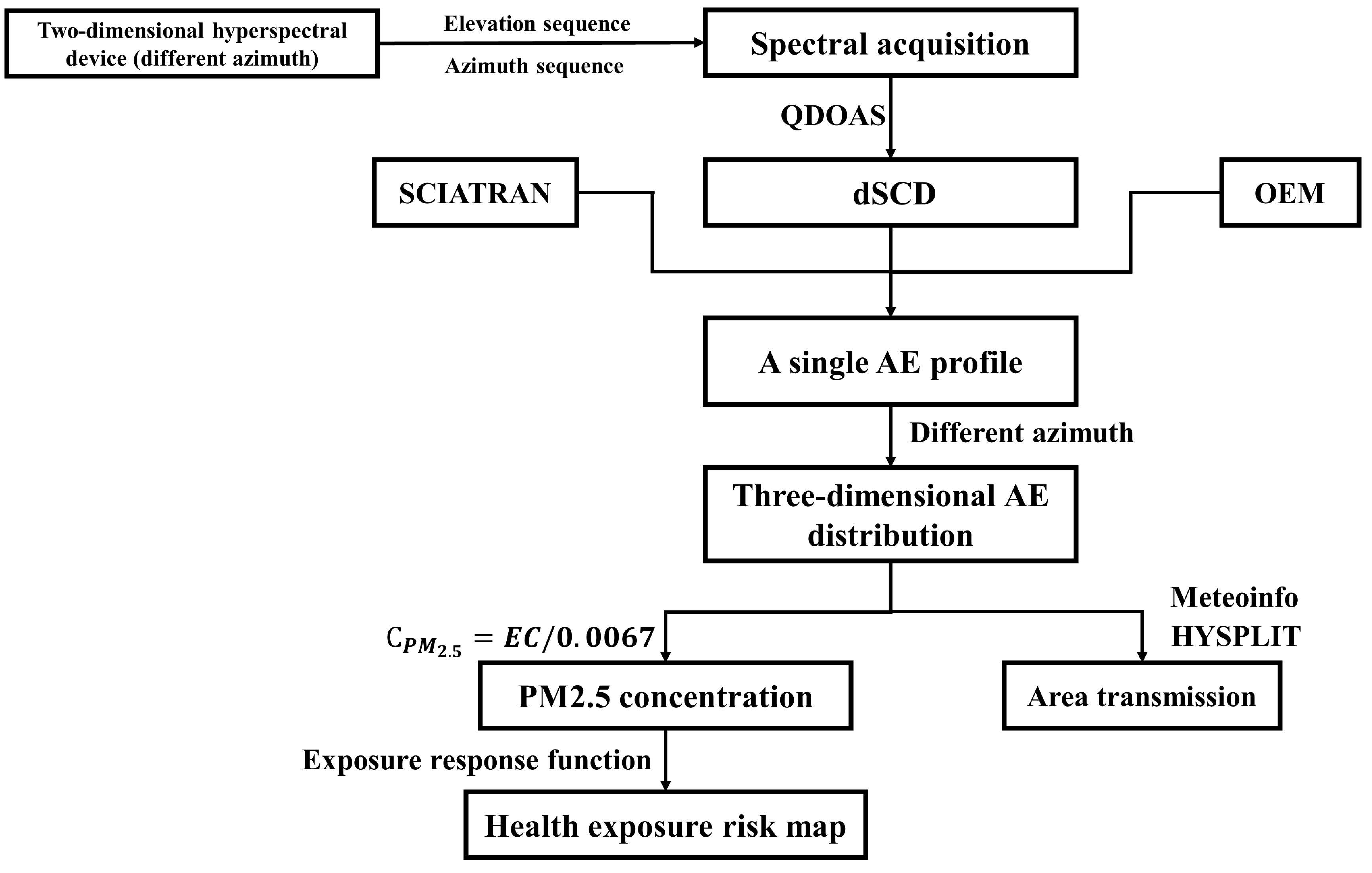
Figure 2.
The schematic diagram of instrument observations. (a) represents all the azimuth angles of the instrument’s observations, and (b) shows the elevation sequence at each azimuth angle. In panel (a), the pentagram symbols indicate the locations of in-situ monitoring stations, while the GPS markers represent the positions of the hyperspectral instrument.
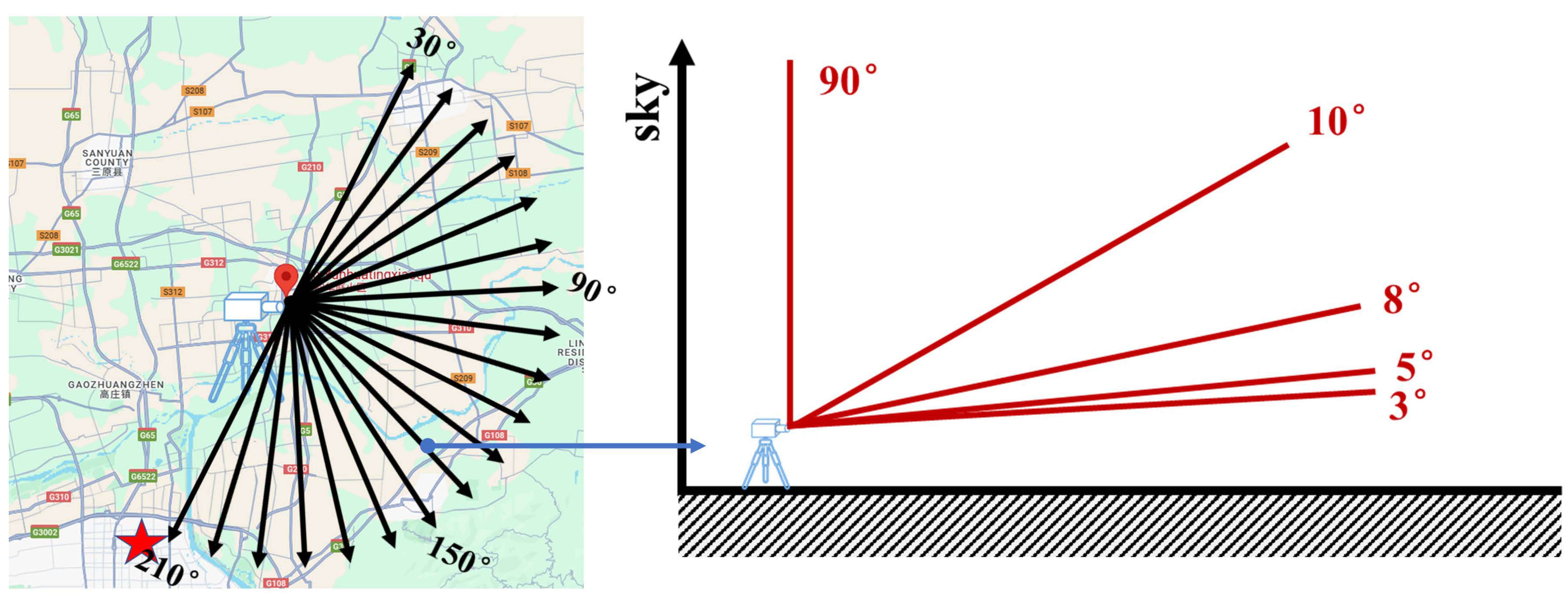
Figure 3.
Example diagram of O4 fitting results.
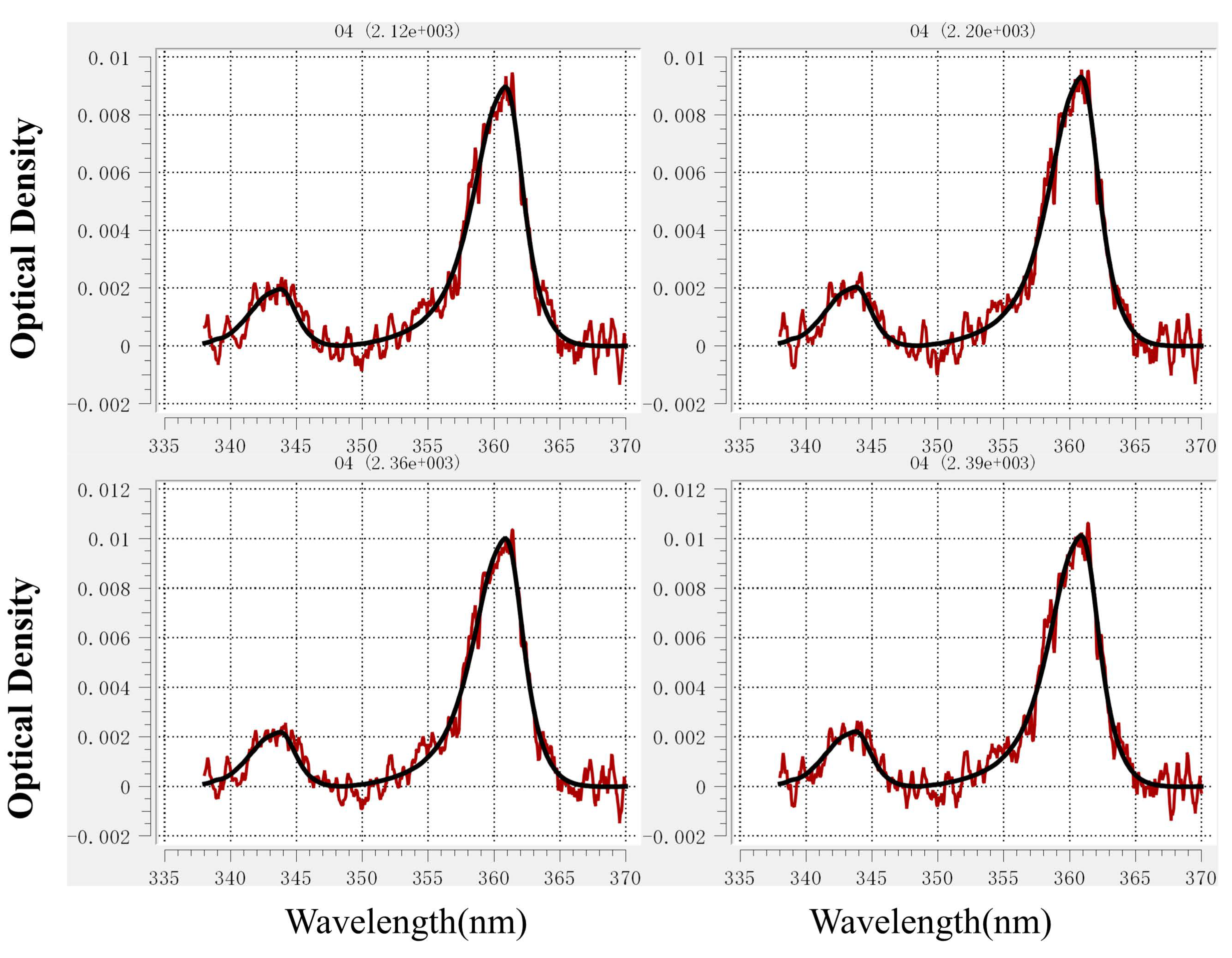
Figure 4.
Comparison of hyperspectral bottom extinction and CNEMC PM2.5.
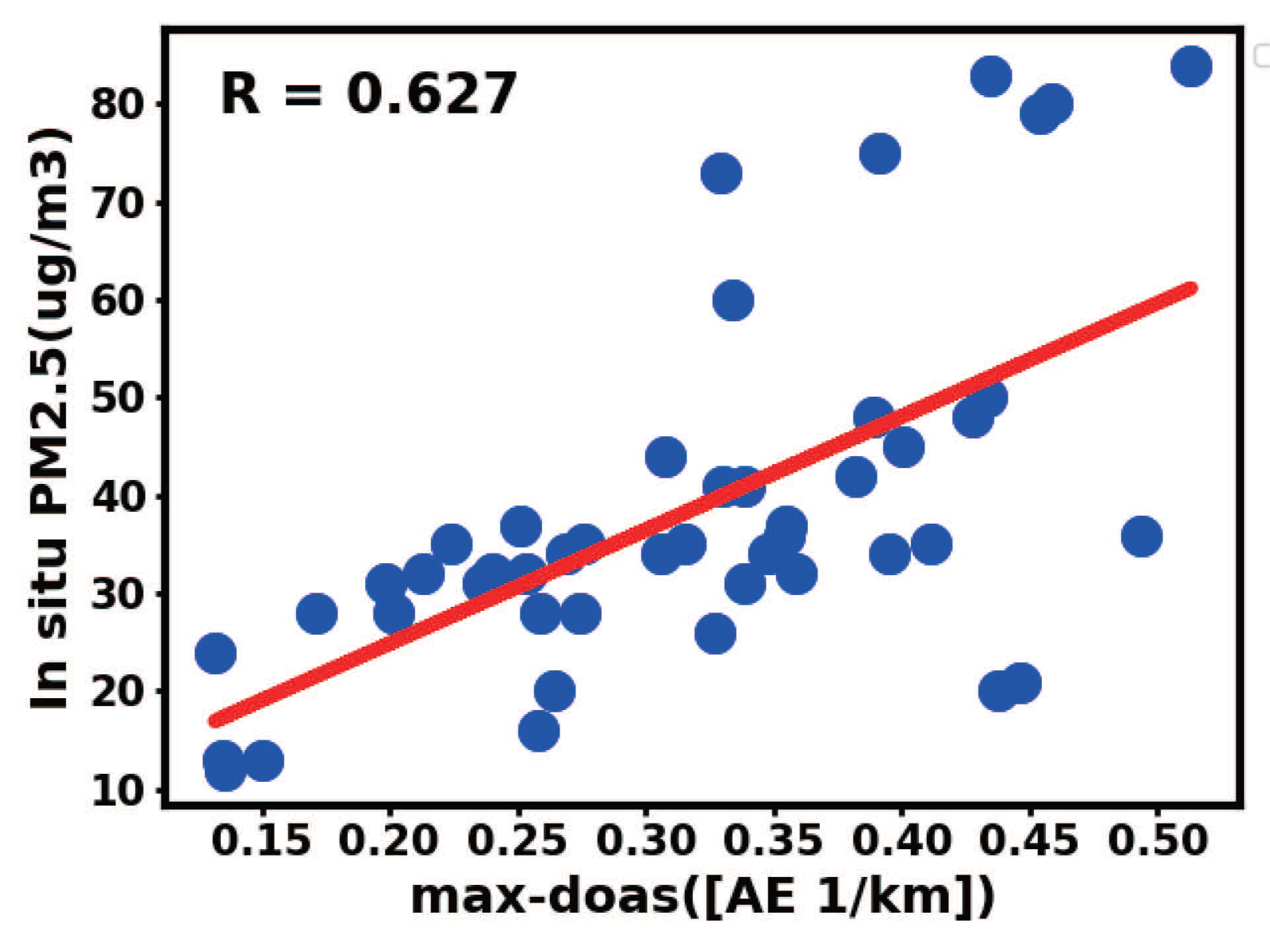
Figure 5.
(a) is the average AE horizontal distribution during the observation time, and (b) is the average AE profile
Figure 5.
(a) is the average AE horizontal distribution during the observation time, and (b) is the average AE profile
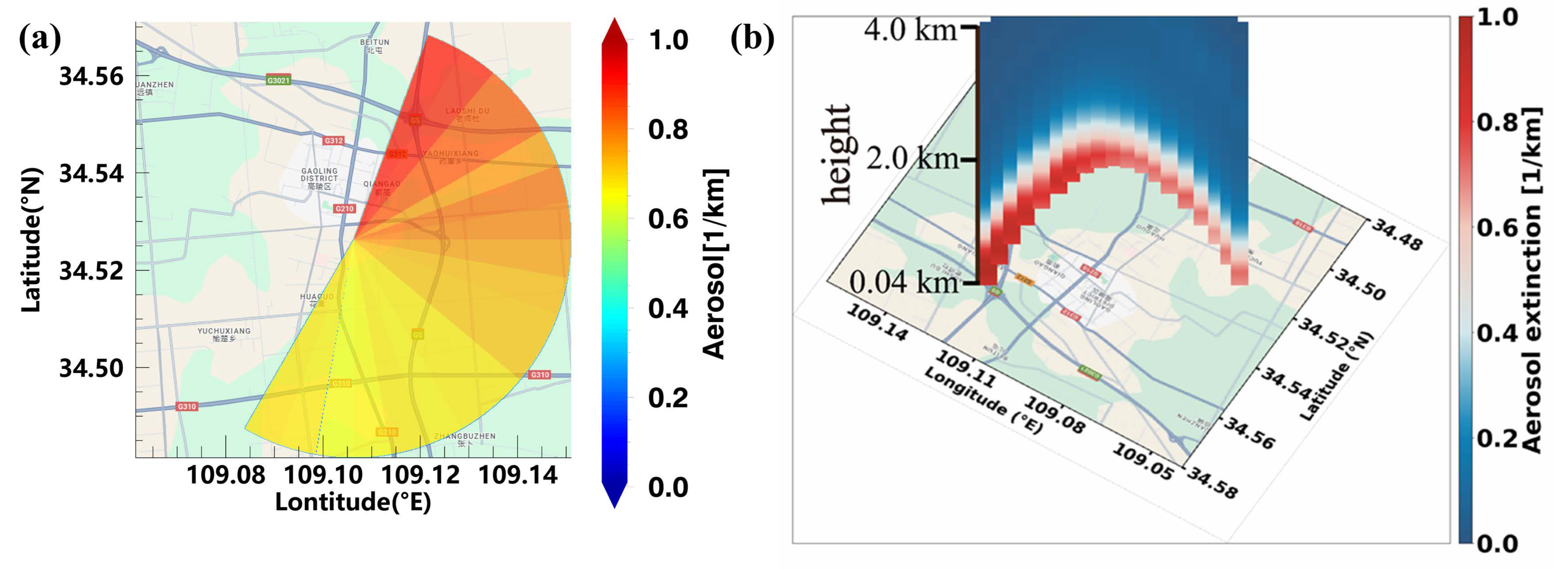
Figure 6.
(a), (b) and (c) are the time average AE profiles at 30°, 100° and 200° azimuths during the observation time, respectively
Figure 6.
(a), (b) and (c) are the time average AE profiles at 30°, 100° and 200° azimuths during the observation time, respectively
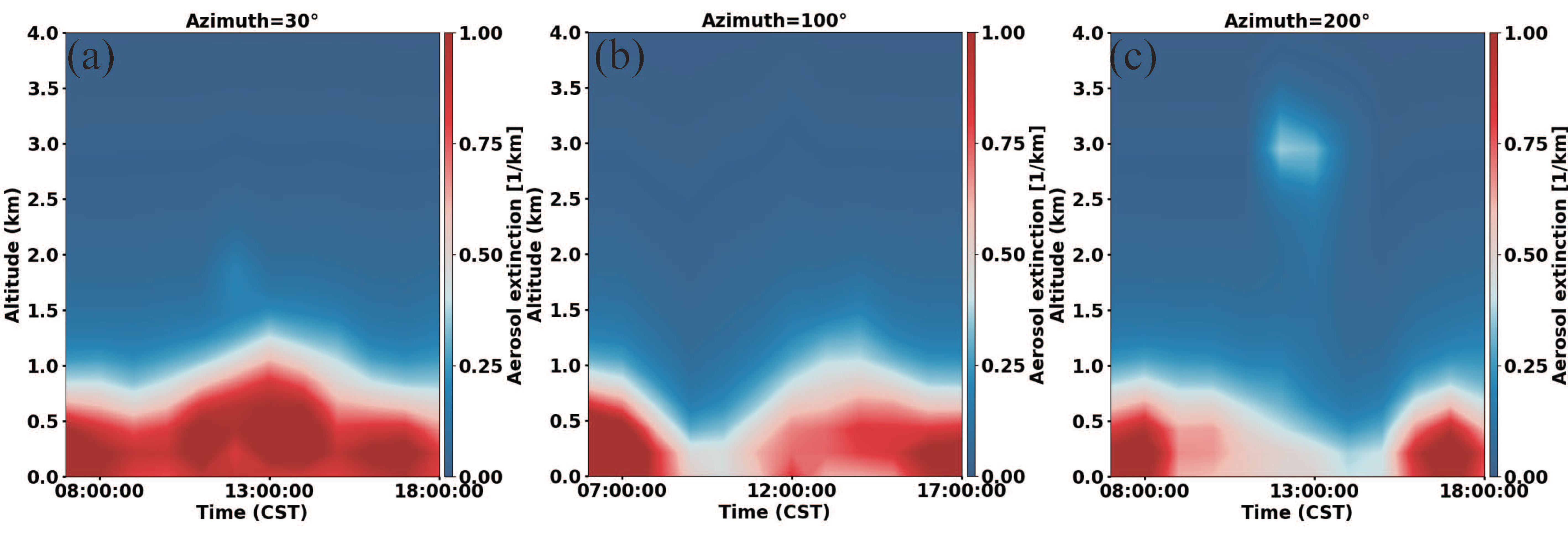
Figure 7.
(a) and (b) show the horizontal and vertical distribution of AE at around 7-8 am on September 25, respectively. (c) shows the satellite screenshot of the overpass, and (d) shows the actual photo of the observation site in the morning
Figure 7.
(a) and (b) show the horizontal and vertical distribution of AE at around 7-8 am on September 25, respectively. (c) shows the satellite screenshot of the overpass, and (d) shows the actual photo of the observation site in the morning
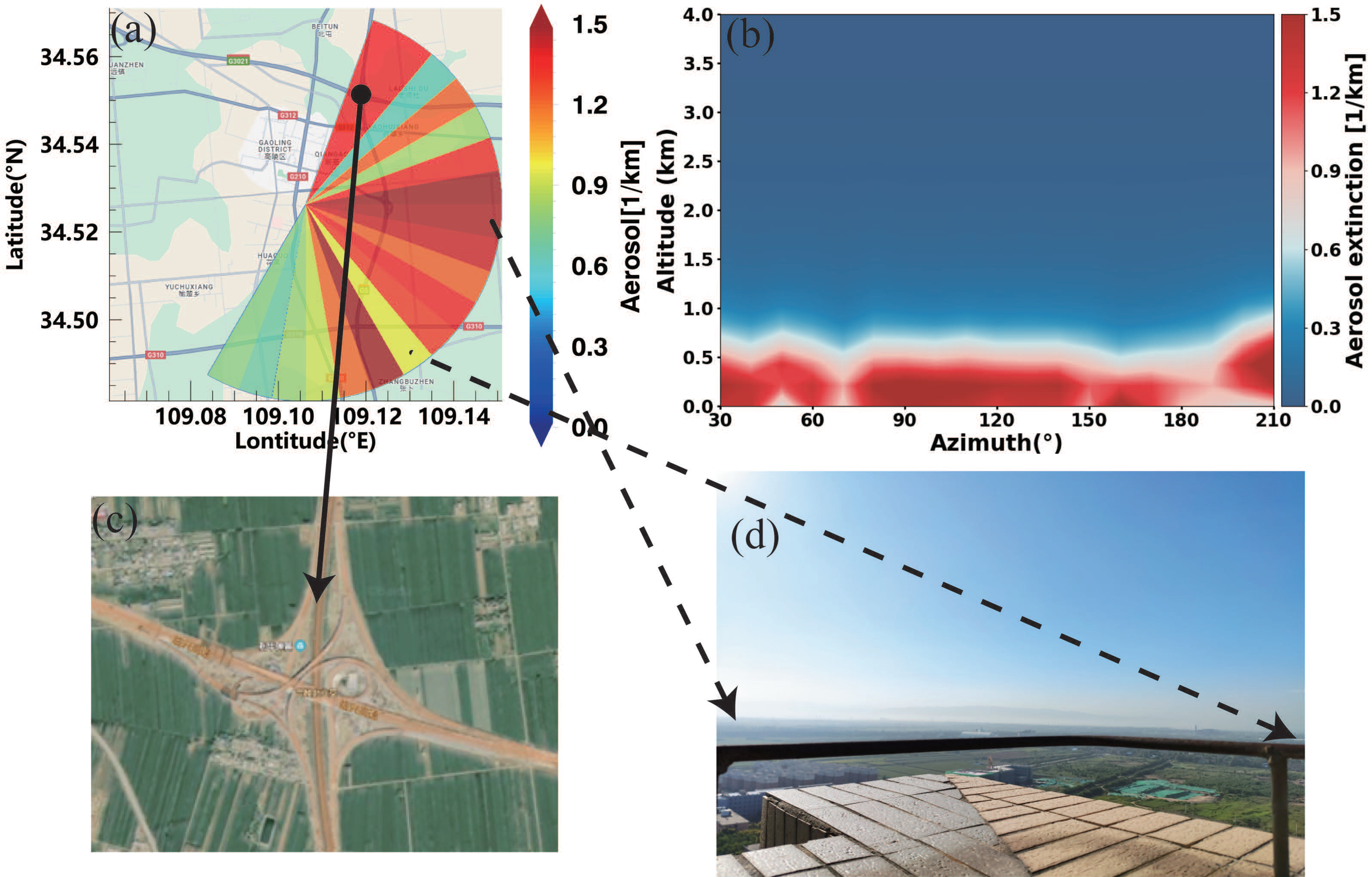
Figure 8.
(a) and (b) show the horizontal and vertical distribution of AE at around 15pm on September 25, respectively, and (c) and (d) show the horizontal and vertical distribution of AE at around 17-18pm, respectively.
Figure 8.
(a) and (b) show the horizontal and vertical distribution of AE at around 15pm on September 25, respectively, and (c) and (d) show the horizontal and vertical distribution of AE at around 17-18pm, respectively.
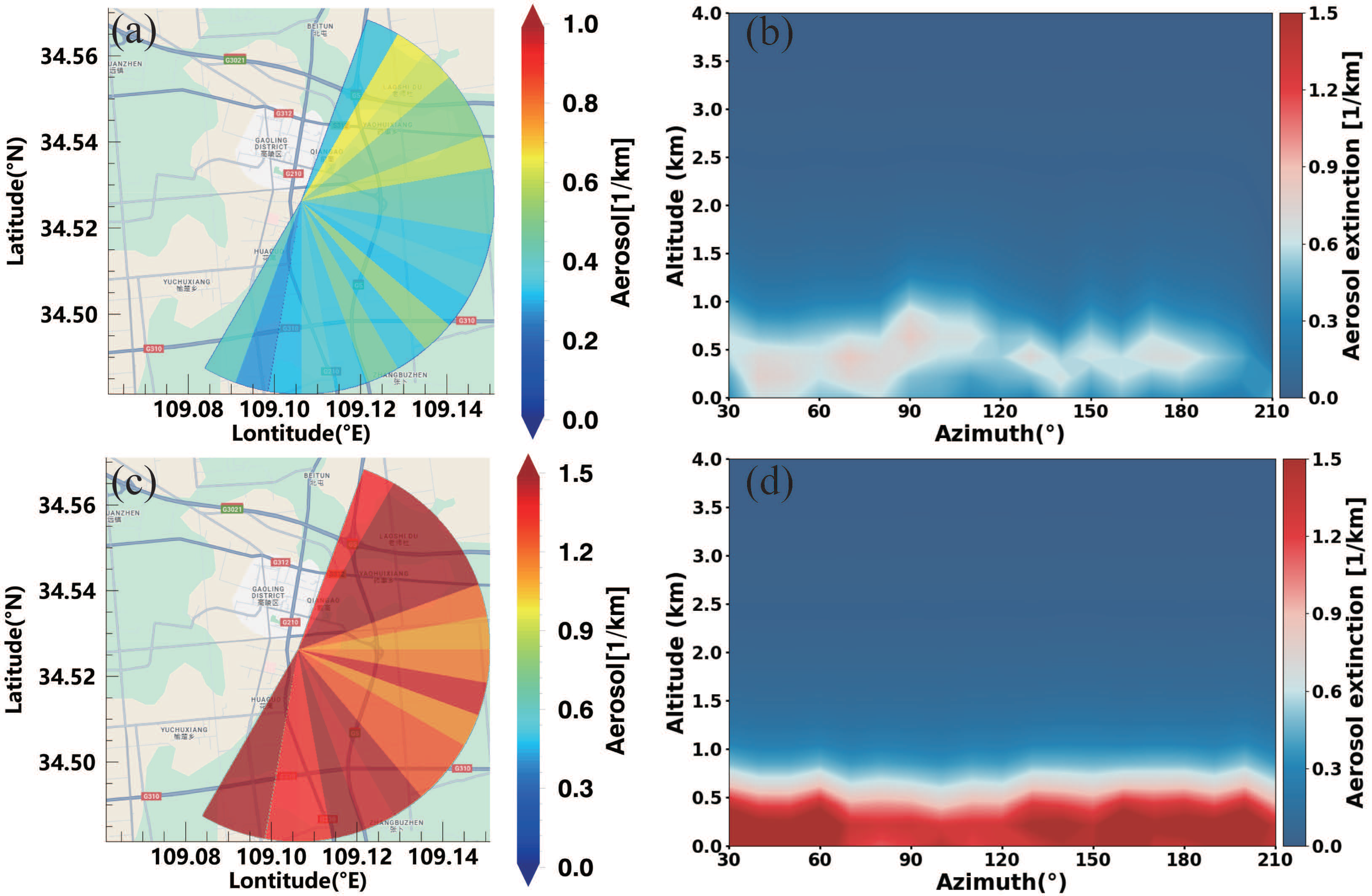
Figure 9.
24h forward trajectory at 40m(a), 200m(b), 400m(c) and 800m(d) altitudes from September to November 2020.
Figure 9.
24h forward trajectory at 40m(a), 200m(b), 400m(c) and 800m(d) altitudes from September to November 2020.
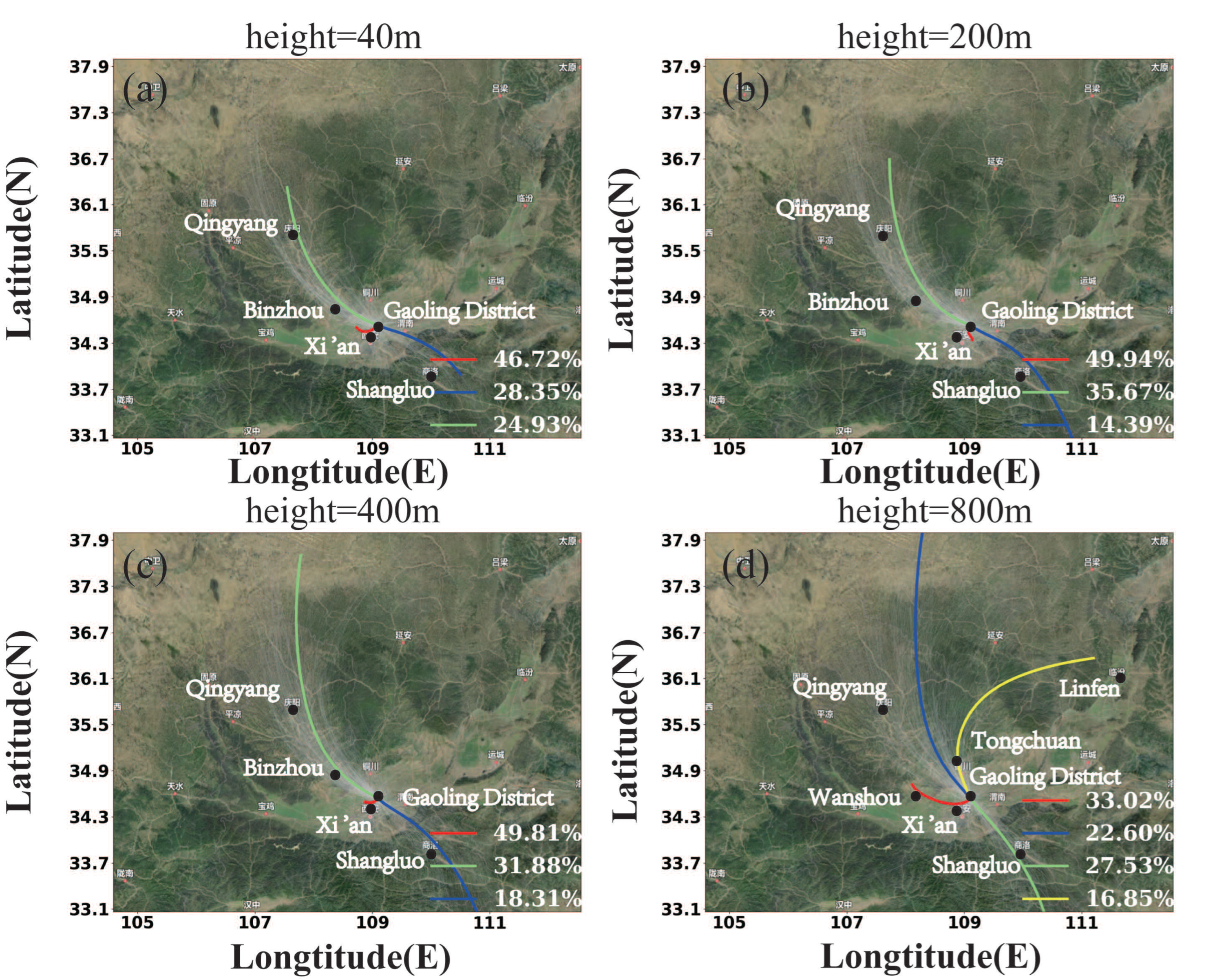
Figure 10.
24h forward trajectory for four altitudes on September 25, 2020.
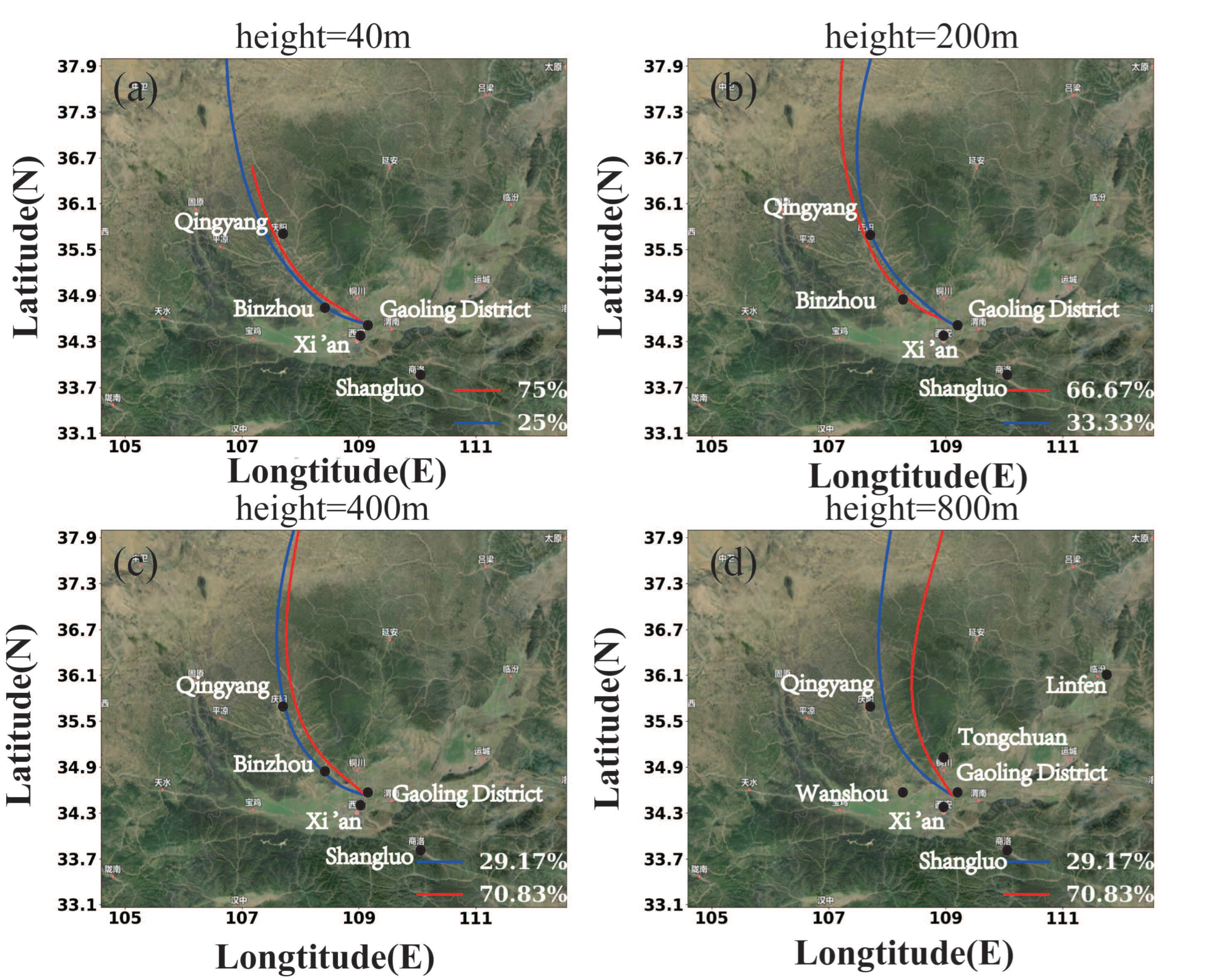
Figure 11.
Horizontal distribution map (average values) of particulate matter air pollution-related case numbers in Gaoling District, Xi’an, from September to November 2020. Panels (a), (b), (c), and (d) represent all types of diseases, RASDs, acute bronchitis, and asthma attacks (children <15 years), respectively.
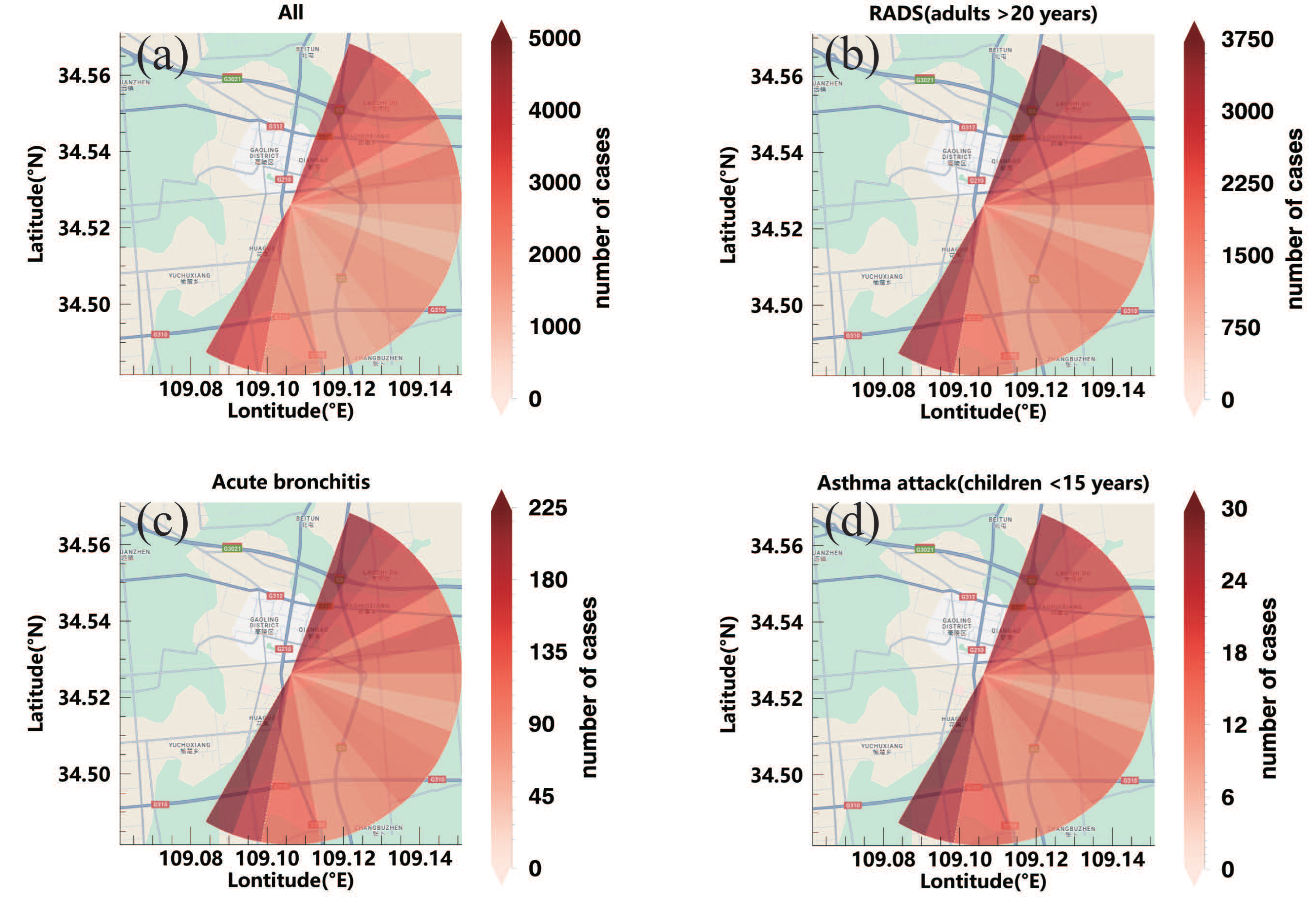
Table 3.
Cases of particulate air pollution in Gaoling District, Xi’an from September to November 2020.
Table 3.
Cases of particulate air pollution in Gaoling District, Xi’an from September to November 2020.
| Health Outcome | Number of cases(average) | |
| Mortality | Long-term | 52 |
| Short-term | 2 | |
| Asthma attack | children < 15 years | 344 |
| adults > 15 years | 241 | |
| Chronic bronchitis | 71 | |
| Acute bronchitis | 2652 | |
| Respiratory hospital admission | 16 | |
| Cardiovascular hospital admission | 11 | |
| Outpatient visits-internal medicine | 1022 | |
| Outpatient visits-pediatrics | 108 | |
| RADs (adults >20 years) | 41678 | |
| Sum | 46107 | |
Disclaimer/Publisher’s Note: The statements, opinions and data contained in all publications are solely those of the individual author(s) and contributor(s) and not of MDPI and/or the editor(s). MDPI and/or the editor(s) disclaim responsibility for any injury to people or property resulting from any ideas, methods, instructions or products referred to in the content. |
© 2025 by the authors. Licensee MDPI, Basel, Switzerland. This article is an open access article distributed under the terms and conditions of the Creative Commons Attribution (CC BY) license (http://creativecommons.org/licenses/by/4.0/).
Copyright: This open access article is published under a Creative Commons CC BY 4.0 license, which permit the free download, distribution, and reuse, provided that the author and preprint are cited in any reuse.


