
Submitted:
02 May 2025
Posted:
29 May 2025
You are already at the latest version
Abstract
Neural Ordinary Differential Equations (NODEs) have garnered significant attention due to their ability to achieve memory savings and to model continuous data. However, NODE-based models suffer from undesirable impacts of adversarial attacks and perturbations, i.e., various types of noise injection, resulting in severe performance bottlenecks and degradations. Herein, we propose a novel improved approach, called Alternate Propagating neural Ordinary Differential Equations (APODE), to tackle the vulnerability of NODEs. Our APODE is proposed to learn representations by an alternate propagating strategy for traditional NODEs, which verifies the robustness of cooperative modelling with more than one dynamic function. The proposed APODE trains an ensemble within two dynamic functions to model the derivative of representations, resulting in alleviating the vulnerability issue and improving the robustness of NODEs. Unlike other ODE-based models, APODE is a simple method that aims at efficiently enhancing robustness against input perturbations and adversarial attacks. Empirical experiments on a wide variety of tasks demonstrate the superiority of our APODE over baseline models in terms of robustness and expressive capacity with a performance improvement of 9.9%~21.6% under adversarial attacks in Cifar10 dataset.
Keywords:
neural network
; neural ODEs
; robustness
1. Introduction
Neural Ordinary Differential Equations (NODEs) [1,2,3], as a type of neural networks that approximate nonlinear mapping in modelling real-world data, offer several advantages such as invertibility and energy efficiency over the traditional neural networks. NODEs are adopted by researchers to reduce the memory usage that is greatly consumed by traditional neural networks [4]. Due to their special structure, NODEs take advantage of a dynamic function [3], a neural network for describing the derivative of representations, to obtain the representations by solving ordinary differential equations (ODEs). NODEs can be interpreted as continuous equivalents of ResNets with no need for intermediate variables and they solve ODEs by ODE solvers, e.g., Euler solver, and therefore save intermediate memories [3] and are suitable to handle a number of memory-saving demanding tasks, e.g., classifications tasks [5] in edge devices, and continuous time modelling tasks [6], e.g., time-series trajectories reconstruction [7].
Despite the success of NODEs in many applications, they still lack model robustness [8,9]. While recent studies [8,10] have shed light on the inherent stability of ODEs compared to traditional neural networks, it is important to note that NODEs still suffer from significant vulnerabilities. The output of NODEs is proved to be sensitive to the noise when modelling data [9,11], making existing NODEs susceptible to input perturbations and adversarial attacks.
To gain a better understanding of modelling vulnerabilities in NODEs, we provide the following specific examples. Indeed, even a minor perturbation can result in significant changes to the output of NODEs [9]. Suppose we have a 1-dimensional (1d) toy example with being the hidden representation and being the standard Brownian motion. Notice that the dynamic function f is the derivative of . When introducing different values of , the behaviour of is noticeably disrupted in comparison to the case when . As shown in Figure 1(a), it is found that noises cause severe changes in . The vulnerabilities of NODEs lead to inconsistent shifts, particularly in cases of severe deviations in output values, rendering NODEs susceptible to adversarial attacks. However, less attention has been paid to exploring the adversarial attacks and robustness of NODE-based networks, resulting in that the urgent exploration of robustness in the NODEs community is still in its infancy.
Ensemble training defends against adversarial attacks by diversifying vulnerabilities among sub-models while maintaining accuracy performance similar to standard training methods [12]. While deploying an ensemble, which is an aggregation of multiple sub-models, weakens NODEs’ advantages of energy and memory efficiency, we propose an Alternate Propagating neural ODE model, abbreviated as APODE, which utilizes an alternate propagating strategy with two learnable dynamic functions to fit the data distribution. Despite employing two dynamic functions, APODE incurs the same computational cost as a single dynamic function. During the forward propagation process, our APODE alternately selects one of two dynamic functions and at each step in solving ODEs to derive the hidden representations of data. This indicates that auxiliary paths are constructed at each step of ODEs. Through this method, APODE is able to generate a multitude of sub-models by randomly sampling, thereby facilitating the training of an ensemble. As shown in Figure 1(b), it can be seen that the hidden representation of APODE is sandwiched between those of two dynamic functions and as a weighted mean (theoretical analysis in Corollary 1), which proves that training APODE is an equivalent method of training an ensemble of NODEs. Theoretical and experimental validations have confirmed that APODE surpasses models that solely employ a single dynamic function in terms of advantages on robustness in NODEs and especially benefits for better generalization and performance to tackle modelling imperfection in traditional NODEs. We make the following explanations of our APODE.
Explanations for Better Model Robustness. Actually, the vulnerability of models generally stems from their excessive certainty [12]. Previous methods [13,14,15] aim to introduce uncertainty and undermine the certainty of models, thereby enhancing their robustness. Pinot et al. [12] has argued that randomized defence strategies tend to be a suitable alternative to defend against strong adversarial attacks. In line with previous methods, our proposed APODE incorporates uncertainty through its alternate propagating strategy. Therefore, we can observe that deterministic NODEs are prone to be disturbed, while our APODE achieves better robustness. Moreover, because the ensemble techniques have been shown to greatly enhance model robustness [12], our APODE benefits from it and tends to exhibit increased robustness, effectively mitigating vulnerabilities that can arise from excessive certainty in models. Furthermore, by adopting a game-theoretic point of view [12], the robustness of APODE can be viewed as an infinite zero-sum game [16] with randomization. Our proposed APODE, incorporating a mixed strategy, is a non-deterministic algorithm that effectively minimizes adversarial risk. Compared with widely recognized Neural SDE [9], our APODE presents more prominent robustness.
Explanations for Better Expressive Capacity. In addition, there exist constraints on the expressive capacity of NODEs [17,18]. For example, it is difficult for existing NODEs to fit the distribution of concentric annulus datasets [17] which can be found in, e.g., Proposition C.6 in [19]. We prove theoretically that our APODE obtains a weighted result of multiple possible models and the usage of two dynamic functions introduces the complex expressive capability by preventing models from learning ordinary results so as to learn more sufficient information. As a result, APODE exhibits superior expressiveness as it can solve the concentric annulus problems [17], while traditional NODEs fail to do so.
Note that APODE only uses two dynamic functions to fit the data distribution. Actually, our APODE can be easily extended to multiple dynamic functions, which we refer to as Multi-APODE. However, Multi-APODE will cause insufficient training and become more randomized with the increased number of dynamic functions. Hence, APODE only uses two dynamic functions as a representative model since we empirically found that this can achieve satisfactory performance.
In summary, we make the following contributions:
- We propose an Alternate Propagating neural ODE model, namely APODE, which has achieved better robustness against one-dynamic-function-based NODEs.
- We provide theoretical proof and conduct experiments to verify that APODE improves expressive ability than traditional NODEs.
- We conduct experiments on classification and regression tasks to verify the effectiveness of APODE. Experimental results demonstrate that our APODE excels in achieving better robustness.
2. Preliminaries
NODEs represent the derivative of the hidden representation with a single neural network as:
where denotes the hidden representation of the model at time step t, f denotes a dynamic function defined by a neural network to describe the derivative of the hidden representation, w.r.t. time t, and represents the parameters in the neural network. The output of a NODE model is calculated using an ODE solver (e.g. the Euler solver) coupled with an initial value problem (IVP):
where and are the initial time point and the ending time point, respectively; and and represent the hidden representation at and , respectively.
NODEs for regression and classification. In NODEs, we map an input (d denotes the dimension of the data) to an output to learn a set of representations by solving an ODE starting from x. NODEs are dimension-preserving mappings and thus we define an extra layer from for practical applications, e.g., regression and classification. The robustness of NODEs can be evaluated through the classification performance on the perturbed dataset. We also conduct experiments with perturbations, namely, random Gaussian noise and harmful adversarial examples to demonstrate our robustness.
3. Related Work
Robustness of NODEs. Due to the vulnerabilities of NODEs, NODEs are suffering from perturbations and adversarial attacks. Even subtle noises can lead to significant alterations in the results achieved [8,9]. Several studies have been conducted to investigate the robustness properties of NODEs, such as Neural SDE [9], which remains high computational cost [20]. Besides, Yan et al. [8] removes the time dependence of the dynamics in an ODE and imposes a steady-state constraint on integral curves, resulting in a large decrease in the ability to obtain dynamic information. Compared with these methods, we leverage an alternate propagating strategy to randomize the solution in ODEs, resulting in that the vulnerabilities is weakened among different paths. Our APODE introduces randomness to alleviate the vulnerability and has proved the superior improvement of robustness in experiments.
Ensemble Networks. Ensembles of neural networks benefit from combining the superiorities of several models to achieve better robustness by averaging or majority voting on the output of each ensemble member [21,22,23]. Most recently, Cai et al. [24] propose structural randomness in neural networks, verifying that the model maintains better robustness gains while greatly reducing training costs. However, the aforementioned works are not applicable to ODE-based models, since its special model structure. We introduce an "implicit" ensemble, which is quite different from traditional explicit time-consuming ensembles. Our APODE model takes into consideration of multiple paths, which can be interpreted as creating an exponential number of weight-sharing sub-networks resulting in being equipped with properties of superior performance [21].
4. Model Architecture
Compared with the existing NODEs that only leverage a single dynamic function to represent the derivative of hidden representations, our APODE describes the derivative of hidden representations with two dynamic functions. In the forward propagation process, our APODE applies an alternate propagating strategy, i.e., select one of two dynamic functions at each time interval, to obtain the output representation. In this section, we introduce the details of our APODE model and provide theoretical analysis to justify the superiority of our APODE over the traditional NODE models. Figure 2 illustrates the architecture of our APODE.
4.1. Alternate Propagating Neural ODEs
In our APODE, we propose to describe the derivative in the ordinary differential equation, i.e., Equation (1), with two dynamic functions, represented as and respectively, which can be different in structures. Specifically, the output representation of our model is given by:
where and are the parameters of the two dynamic functions and , respectively, is the initial hidden representation, and g denotes an alternate propagating strategy function, which is defined as:
where for the sake of discussion, we use and to represent and , respectively, and is an indicator function specifying how to choose a dynamic function at time t, which is defined as:
where is a randomly sampled variable at each time step t, and is a hyperparameter for defining the alternate propagating strategy function g. Particularly, we can regard p as the probability of choosing the dynamic function , i.e., the probability of choosing is . At each time interval of the forward propagation process, our APODE propagates using the dynamic function with probability p and propagates using the dynamic function with probability . We refer to a possible propagation trajectory from to as a path. For example, a possible propagation path from to is shown in Figure 3(a). Since our APODE selects one dynamic function for propagation with probability p at each time step, it implicitly constructs auxiliary paths over possible paths from to . Therefore, our proposed APODE can be regarded as a collection of multiple paths as shown in Figure 3(b). There are possible propagation trajectories in our APODE from initial time step to ending time step , where n is the approximate number of time intervals between and , and our APODE can be thought of as implicitly instantiating sub-models on all possible selections.
Randomization Matters in Presenting Robustness. The main impact of APODE lies in its ability to facilitate the integration of collective capabilities and eliminate vulnerabilities by inducing sub-models with diverse paths to counteract attacks. Through harnessing the integration of these capabilities across multiple paths, APODE showcases a remarkable level of flexibility and expressiveness. In fact, APODE effectively isolates adversarial vulnerabilities by employing multiple paths, thereby significantly reducing the attack capabilities of attackers among sub-models [25]. Intuitively, an adversarial sample would need to deceive the majority of numerous models in a well-trained APODE-based model, which proves to be an exceptionally challenging task. Furthermore, APODE also benefits from randomization to encourage generalization by inducing sub-models with diverse paths against attacks.
By adopting a game-theoretic point of view [12], the robustness of APODE can be viewed as an infinite zero-sum game [16] with randomization. Randomization has been argued to be a suitable alternative to defend against strong adversarial attacks [12]. Indeed, numerous studies [14,15] have verified that noise injection can offer a verifiable defence mechanism against adversarial attacks. Actually, a connection can be established between these studies and our proposed APODE approach by recognizing that a classifier injected with noise can be perceived as an infinite combination of alternate classifiers of APODE. Therefore, our APODE exhibits a high level of robustness. Additionally, we are well aware that the interaction between the Defender and the Adversary in a point-wise attack scenario can be likened to a two-player zero-sum game. In such a game, the Defender strives to design a classifier that performs optimally under attack, while the Adversary aims to devise the most effective attack for that specific classifier in every instance. The selection of a classifier f (referred to as a strategy for the Defender) or an attack (referred to as a strategy for the Adversary) is pivotal in adversarial topics. Notably, Pinot et al. [12] demonstrate that there exists no pure Nash equilibrium, which gives arguments for using randomization. This implies that no deterministic classifier can withstand every attack, and that any deterministic classifier can be outperformed by a classifier that incorporates worst-case randomness. Furthermore, they point out that the efficacy of any deterministic defence can be enhanced by adopting a simple mixed strategy. This approach bears resemblance to the fictional game concept in game theory [26] and the facilitative concept in machine learning [27]. The same principle holds true in APODE as well.
Comparison to Traditional Ensemble Methods. The proposed APODE implicitly contains multiple propagation trajectories, i.e., paths. By selecting paths between two dynamic functions, our APODE trains an ensemble in the forward propagation process, and consequently it presents the ensemble robustness during inference [24]. Traditional ensemble models combine multiple sub-models to jointly make decisions which lead to high memory usages [28,29]. However, our APODE instead incurs the same computational cost as a single dynamic function and offers the same advantage as ensembles in achieving superior performance through comprehensive diversification of representations [21]. APODE can be viewed as an "implicit" ensemble and the set of multiple paths can improve the robustness of the ODE-based models. Furthermore, APODE shows better capabilities than traditional NODEs, such as improving the expressive capacity of ODE-based models and enhancing their robustness. Different from traditional ensemble models, which have poor scalability owing to the increased model complexity when including more sub-models, APODE simply increases the number of paths, which is equivalent to mitigating training cost.
4.2. Insights into the Properties of APODE
APODE surpasses traditional NODEs in terms of expressive ability and robustness, and we provide the analysis in this subsection. We first point out the performance limitations of traditional NODEs in Theorem 1, then analyze the average hypothesis of APODE as an ensemble in Corollary 1, and finally explain its robustness.
Usually, in traditional NODEs, the ODE modules learn an informative feature map from the training data to make predictions, and after that a nonlinear mapping is performed on the resulting feature map. They have limitations in their expressiveness that they even could not classify simple concentric annulus datasets due to Theorem 1:
As is widely recognized, Theorem 1 represents a significant limitation of traditional NODEs. This limitation restricts their ability to learn complex distributions, resulting in subpar performance in such scenarios [17]. As shown in Figure 4(a), suppose a 1d toy example, continuous trajectories mapping -1 to 1 and 1 to -1 from to must intersect each other (i.e., the line connecting (, -1) and (, 1) and the line connecting (, 1) and (, -1) must intersect at a certain point within the interval [, ]), which is not possible for an ODE [17]. Considering a 1d input in APODE wherein the state is a scalar as shown in Figure 4(b). By Theorem 1, the traditional NODE is limited in that the solution curve is always sandwiched between two solution curves from to throughout time resulting that it being difficult for the NODE-based model to learn complex distributions, e.g., the concentric annulus datasets. Contrarily, Equation (3) of our APODE can break through the expressiveness limitations. We suppose that there has three solutions , from the dynamic functions and , and from the dynamic function . starts from , where is the feature of an input. Suppose that is between and as , where , , and , present two features of independent inputs. Actually, during the time from to , by the alternate propagating method of APODE, the solution curve with the dynamic function g has chances to surmount the limit of sandwiching between the integral curves and . Consider at the timestamp and and where , then APODE altenate propagates to at and , simultaneously, such that . Thus, our APODE has the opportunity to surpass limitations of that ODE solution curves do not intersect in Theorem 1 and acquire more generalized representations from the function g and learn more complex mappings than traditional NODEs [17].
We next aim to show that, APODE ensures that the expectation of feature maps lies between their independent feature map from two dynamic functions as an ensemeble.
Corollary 1.
Let and denote two dynamic functions in NODEs and g denotes an alternate propagating dynamic function. Then it holds that the integral expectation of g is sandwiched between the integral expectations of and , such that is sandwiched between and , where .
Through Theorem 2 and Theorem 3 as follows, we theoretically analyze the Corollary 1 that APODE can bridge the gap of estimation error in existing ways to achieve an ensemble learning during training, in other words, the model output obtained at time is sandwiched between the respective outputs of two dynamic functions and .
Theorem 3. (The Mean Value Theorem for Integrals [31]) There exists a value in the interval and the dynamic function f is continuous, such that .
By performing multiple sampling of t within the interval , we can establish that the expected integral value of the first term in Equation (4) is equivalent to
Similarly, the expected integral value of the second item in Equation (4) holds that . At time , denotes the initial value of APODE, and the expected integral value obtained by our APODE holds that . Particularly, when p is equal to 1, the increment of becomes . Similarly, when p is equal to 0, the increment of becomes . This implies that the APODE model reverts back to a traditional NODE.
Overall, it holds that the expected integral value of g is sandwiched between the expected integral values of and by Corollary 1. Coherent to average hypothesis theory[32,33], the outputs of APODE, are an ensemble derived from both and . Such that is sandwiched between and , where .
To argue the robustness of APODE, we demonstrate a significant level of robustness, as evidenced by the proof provided earlier that APODE achieves robustness within an ensemble approach. Existing researches have also affirmed that ensemble greatly enhances model robustness [12]. Furthermore, our APODE, incorporating a mixed strategy, is a non-deterministic algorithm that effectively minimizes adversarial risk.
To be precise, the goal of an Adversary is to find the perturbation that maximizes the adversarial risk defined as follows:
where denotes data pairs from datasets . Therefore, in this zero-sum game, a strong Adversary is manipulating the dataset distribution:
It means that the Adversary tries to find to satisfy ; while the Defender tries to find to satisfy . What has been proved that randomization for both players indeed helps improve model robustness. In particular, our proposed APODE tends to maintain a new objective function written as:
where APODE introduces a mixture of classifiers of the Defender. As proved in Corollary 1, APODE can be viewed as a sampling ensemble method. In APODE, giving some input features x, this amounts to picking a classifier in each step from at random, and then uses it for ODE calculation to output the predicted class, i.e., . Note that the Defender’s mixed strategy is a non-deterministic algorithm because it relies on a sampling of . Thus, even if the attack is defined in the same way as before, the adversary now needs to maximize , in other word, the adversary needs to maximizes the adversarial risk of each path under the distribution . As proved in [12], it is reasonable to conclude that our model possesses better robustness. The rationale behind this idea stems from the fact that, by our ingenious design, a successful attack on either of the two classifiers () will not be effective against the other one. This observation aligns with Theorem 2 in [12], which demonstrates that stochastic algorithms enhance robustness.
The calculation of the corresponding ODE solver in the propagation of APODE at each step is completed in the same dynamic function, and consequently APODE is still Lipschitz continuous. In our experiments, we are still able to use torchdiffeq package1 with modification. As mentioned above, our proposed APODE can be regarded as a combination of multiple sub-models, which can alleviate the likelihood of being attacked than only one dynamic function, and present the strong robustness as well as superior performance as ensemble models.
4.3. Multiple Dynamic Functions of APODE
By Theorems 2 and 3, APODE with more than two dynamic functions (called Multi-APODE) still guarantees average hypothesis theory. Therefore, the model can still work, but the memory cost is too expensive. Meanwhile, Multi-APODE will cause insufficient training and the model will become more randomized with the growth of n. Therefore, we only use two dynamic functions in APODE as a representative model since we empirically found that this can achieve satisfactory performance.
5. Discussion
Exploring the future of attacking APODE presents an intriguing avenue worth investigating. In recent studies, adversarial techniques have been introduced to impair the performance of ensemble models [34]. However, it should be noted that these methods are designed for aggregating the results of individual models and therefore may not be directly applicable to our proposed APODE. Empirical experiments in the following experiments section have demonstrated the superiority of our APODE over these adversarial methods. Hence, it would be worthwhile to design adversarial attacks on our APODE model in our future research.
6. Experiments

Table 1.
Classification accuracy (mean ± std in %) on perturbed images from Mnist, SVHN and Cifar10. In order to verify the robustness of APODE, we use Gaussian noise disturbance, FGSM attack [35] and PGD attack [36].
| Gaussian noise | Adversarial attack | ||||
|---|---|---|---|---|---|
| Mnist | =100 | FGSM-0.3 | FGSM-0.5 | PGD-0.2 | PGD-0.3 |
| CNN | 98.7±0.1 | 54.2±1.1 | 15.8±1.3 | 32.9±3.7 | 0±0 |
| ODENet | 99.4±0.1 | 71.5±1.1 | 19.9±1.2 | 64.7±1.8 | 13.0±0.2 |
| Neural SDE | 98.9±0.1 | 72.1±1.6 | 22.4±1.0 | 70.1±1.1 | 15.5±0.9 |
| TisODE | 99.6±0.1 | 75.7±1.4 | 26.5±3.8 | 67.4±1.5 | 13.2±1.0 |
| SODEF | 99.5±0.1 | 71.5±1.2 | 23.5±1.8 | 69.8±1.4 | 15.5±1.1 |
| SONet | 99.5±0.1 | 72.8±1.9 | 20.4±1.0 | 66.7±0.9 | 13.6±1.0 |
| APODE (OURS) | 99.3±0.1 | 75.7±0.5 | 28.4±1.2 | 77.4±0.4 | 28.9±1.4 |
| TisODE + APODE (OURS) | 99.6±0.1 | 80.4±0.1 | 40.9±1.8 | 78.5±0.1 | 37.5±3.6 |
| Gaussian noise | Adversarial attack | ||||
| SVHN | =35 | FGSM-5/255 | FGSM-8/255 | PGD-3/255 | PGD-5/255 |
| CNN | 90.6±0.2 | 25.3±0.6 | 12.3±0.7 | 32.4±0.4 | 14.0±0.5 |
| ODENet | 95.1±0.1 | 49.4±1.0 | 34.7±0.5 | 50.9±1.3 | 27.2±1.4 |
| Neural SDE | 95.3±0.1 | 56.6±1.1 | 40.8±1.1 | 59.7±0.6 | 42.6±0.3 |
| TisODE | 94.9±0.1 | 51.6±1.2 | 38.2±1.9 | 52.0±0.9 | 28.2±0.3 |
| SODEF | 95.0±0.1 | 55.1±1.1 | 38.8±1.5 | 59.9±0.9 | 33.6±0.7 |
| SONet | 94.8±0.2 | 52.3±0.8 | 36.9±0.9 | 55.7±1.4 | 30.5±0.9 |
| APODE (OURS) | 95.9±0.2 | 58.3±0.2 | 42.6±0.7 | 70.2±0.3 | 49.1±0.4 |
| TisODE + APODE (OURS) | 93.2±0.1 | 58.8±0.1 | 44.2±0.1 | 69.5±0.1 | 50.2±1.6 |
| Gaussian noise | Adversarial attack | ||||
| Cifar10 | =35 | FGSM-5/255 | FGSM-8/255 | PGD-3/255 | PGD-5/255 |
| CNN | 72.2±0.3 | 16.5±1.0 | 6.0±0.4 | 29.8±1.5 | 11.4±0.9 |
| ODENet | 73.5±0.2 | 20.0±0.7 | 9.3±0.1 | 30.8±1.1 | 13.2±0.4 |
| Neural SDE | 72.8±0.2 | 22.7±0.1 | 14.1±1.0 | 33.9±1.3 | 19.3±0.7 |
| TisODE | 73.2±0.4 | 19.6±0.5 | 8.4±0.3 | 30.8±1.2 | 12.2±0.9 |
| SODEF | 73.8±0.2 | 21.3±0.3 | 10.7±0.3 | 37.4±1.0 | 25.1±0.8 |
| SONet | 73.9±0.4 | 22.8±0.4 | 11.4±0.6 | 35.1±0.8 | 23.7±0.6 |
| APODE (OURS) | 74.3±0.3 | 29.5±0.7 | 16.2±0.2 | 50.8±1.6 | 33.8±0.7 |
| TisODE + APODE (OURS) | 74.2±0.2 | 30.1±1.4 | 16.2±0.8 | 49.8±0.5 | 32.5±0.2 |
In this section, we evaluate the performance of our APODE in commonly used datasets for regression and classification. We also assess the expressive capacities of our APODE on the concentric annulus datasets [17] and prove our robustness compared to existing models, including CNN, traditional NODE (ODENet) and their variants [3,9,17], TisODE [8], and most recent methods SODEF [10] and SONet [37]. We also discover adversarial performance on the most recent attack against ensembles named ARC [34]. As a result, we verify that APODE can achieve better robustness than existing models, and tackle the model limitations in traditional NODEs.
6.1. Experimental Details
Details of datasets. We conduct experiments on the following datasets, which consist of image recognition tasks, 1d and 2d sphere datasets and trajectory reconstruction tasks.
- Toy dataset: We generate trajectories consisting of 50 time points within the interval [0, 5]. We evaluate the performance of APODE in experimental settings where datasets with noise data make up around 10% of the total data. The noise perturbations are sampled from a uniform distribution, with values fluctuating within the range of 0 to 2.
- 1d and 2d sphere datasets: We conduct experiments on two concentric annulus problems, including 1d and 2d sphere datasets.
6.2. Research Questions
In following, we seek to answer these research questions: (RQ1) Can APODE improve robustness against both random Gaussian perturbations and adversarial attack examples? (RQ2) Can APODE yield better performance on concentric annulus problems to improve the expressive capacities of NODEs? (RQ3) Is APODE comparable to ensembles and how to adjust the error bound accordingly by choosing p? (RQ4) Can our proposed APODE resistance to noise disturbances when applied to time-series datasets with noise, e.g., toy examples of time-series datasets?
6.3. RQ1: Robustness Analysis
To answer RQ1, we evaluate our robustness improvement by comparing with CNN model, vanilla NODE, TisODE and most recent methods SODEF and SONet on three commonly used datasets including Mnist, SVHN and Cifar10. We employ the same architectures and experimental settings as in Yan et al. [8]. As shown in Table 1, our APODE consistently outperforms all the baselines and existing state-of-the-art methods, indicating that our APODE is able to effectively improve the robustness of all the ODE-based models. Furthermore, we extend the application of APODE to TisODE, which presents enhancement in robustness. For instance, when considering the Cifar10 dataset, APODE and TisODE+APODE demonstrate a respective increment of 0.4% and 0.3% in robustness against Gaussian noise perturbations, in comparison to the most recent model SONet. In terms of FGSM attacks, APODE showcases an increase of 6.7% and 4.8%, while TisODE+APODE exhibits increments of 15.7% and 10.1% in comparison to SONet. Similarly, for PGD attacks, APODE displays an increase of 7.3% and 4.8%, whereas TisODE+APODE shows increments of 14.7% and 8.8%.
In order to evaluate the robustness of attacks which are specifically designed for ensembles, e.g., ARC attack [34], we conduct experiments to demonstrate our performance in this aspect. As shown in Table 2, herein, we introduce a modified version of APODE specifically tailored for preserving the independent gradient with independent members, aligning it with the requirements of ARC (as APODE* in Table 2). APODE* outperforms APODE by 0.6% in terms of performance under PGD attacks, albeit at a higher computational cost and memory usages. In our experiment, ARC represents an improved version of PGD adversarial models. Additionally, our experiments reveal that our proposed method still maintains a performance advantage of 3.7% over NODEs when subjected to ARC attacks.
6.4. RQ2: Functions NODEs Cannot Represent
To answer RQ2, we conduct experiments on the 1d and 2d sphere datasets, as illustrated in Figure 5. The corresponding results are displayed in Figure 6. As mentioned, we argue that APODE can present a more expressive function than vanilla NODEs. For example, as explained in Theorem 1, the concentric annulus problems cannot be represented by vanilla NODEs due to the limitation of Theorem 1 and the global Lipschitz continuous property.
For the 1d sphere dataset, consider , and let be a function, where the dimension d of input data responses to 1. In case the input x is a one-dimensional value and falls between and , the function g assigns a label of 0 to this input (referred to as region A in Figure 5(left)). Similarly, when the input x is between and , the function g assigns a label of 1 to this input (referred to as region B in Figure 5(left)). As Dupont et al. [17] mentioned, vanilla NODEs cannot represent since the region of class 0 is enclosed by the region of class 1, and points of class 0 must cross over the region of class 1 to become linearly separable. Similarly, for the 2d sphere dataset, consider , and let be a function that vanilla NODEs cannot present [17]. In case the input x is a two-dimensional value and the Euclidean norm of the input x is less than , the function g assigns a label of 0 to this input (referred to as region A in Figure 5(right)). Similarly, when the Euclidean norm of the input x is between and , the function g assigns a label of 1 to this input (referred to as region B in Figure 5(right)), respectively.
In order to illustrate the expressive capacities of our APODE, we prove that our proposed APODE represents more complex functions than vanilla NODEs. By examining the loss plots depicted in Figure 6 for both vanilla NODEs and APODE on the 1d and 2d sphere datasets, it becomes evident that vanilla NODEs struggle to accurately map the sphere datasets. Conversely, we observe that APODE excels at approximating these functions effectively.
6.5. RQ3: Examination on Ensemble Property of APODE
To answer RQ3, In our APODE, we introduce a hyperparameter p for defining the alternate propagation strategy function g. To examine how the hyperparameter p affects the performance of our APODE, we conduct experiments on Cifar100 dataset under different settings of p. Specifically, we linearly increase p from 0 to 1, and report the corresponding performance of our APODE. The experimental results are shown in Figure 7(a), which suggests that the performance of APODE peaks when and degrades when p approaches 0 or 1. This can be explained by the fact that when p equals 0 or 1, the proposed method degenerates to vanilla NODEs which propagates with only one dynamic function and thus is unable to achieve better robustness of the input perturbations and adversarial attacks. In addition, our APODE achieves the best performance when p equals , which is equivalent to that our APODE has the maximum amount of paths to choose from because the total number of possible paths is more likely to tend to . Note that the value of n is related to the ODE solver and time step, e.g., the step size is set to 0.05 when Euler’s method is used in our experiments. We utilize Euler’s method in the ODE solver with various step sizes, and all of them yield consistent results.
In order to compare the performance of our APODE with a traditional ensemble which propagates through two respective NODE modules with the same parameters with our APODE. We conduct experiments on Cifar10, Stl10, Cifar100 and F-mnist datasets. As shown in Figure 7(b), APODE obtains similar performance and proves that it exhibits similar properties. Furthermore, APODE saves the computation resources than the ensemble.
6.6. RQ4: Results for Time Series Datasets with Noise
In our APODE, we leverage the alternate propagating method to explore the generalized distribution of training data and reduce the adverse effects of noisy data which is commonly encountered in real-world applications. We conduct the time-series tasks to examine the generalization ability of our APODE. The experiments involved reconstructing complete trajectories from sporadic and irregularly sampled points, encompassing 50 observations with uniformly distributed noise, all within the same training epoch. Comparing the results, we found that Latent ODE+APODE more accurately captures the trajectory, which follows the pattern of , compared to using only Latent ODE, as depicted in Figure 8. This demonstrates the superior performance of our APODE in capturing and modelling complex periodic patterns under severe disruption.
7. Conclusion
In this paper, we propose APODE, a novel improved approach that significantly improves the expressive capacities and robustness than existing ODE models. Our proposed model achieves the improvement through an alternate propagating strategy, which is validated on a diverse range of tasks in our experiments, including concentric annulus datasets, image recognition, and time series tasks. The results confirm that our APODE model consistently outperforms traditional NODEs, demonstrating superior robustness and expressive capabilities. Furthermore, we provide theoretical proof which highlights that our APODE not only enhances the robustness of ODE-based models but also improves overall performance on concentric annulus datasets. These findings underscore the efficacy of APODE in advancing the capabilities and applicability of ODE models.
References
- Ruiz-Balet, D.; Zuazua, E. Neural ode control for classification, approximation, and transport. SIAM Review 2023, 65, 735–773. [Google Scholar] [CrossRef]
- Linot, A.J.; Burby, J.W.; Tang, Q.; Balaprakash, P.; Graham, M.D.; Maulik, R. Stabilized neural ordinary differential equations for long-time forecasting of dynamical systems. Journal of Computational Physics 2023, 474, 111838. [Google Scholar] [CrossRef]
- Chen, R.T.; Rubanova, Y.; Bettencourt, J.; Duvenaud, D.K. Neural ordinary differential equations. Advances in neural information processing systems 2018, 31. [Google Scholar]
- Xu, J.; Zhou, W.; Fu, Z.; Zhou, H.; Li, L. A survey on green deep learning. arXiv 2021, arXiv:2111.05193. [Google Scholar]
- Sun, P.Z.; Zuo, T.Y.; Law, R.; Wu, E.Q.; Song, A. Neural Network Ensemble With Evolutionary Algorithm for Highly Imbalanced Classification. IEEE Transactions on Emerging Topics in Computational Intelligence 2023. [Google Scholar] [CrossRef]
- Wu, Y.; Lian, C.; Zeng, Z.; Xu, B.; Su, Y. An aggregated convolutional transformer based on slices and channels for multivariate time series classification. IEEE Transactions on Emerging Topics in Computational Intelligence 2022. [Google Scholar] [CrossRef]
- Golovanev, Y.; Hvatov, A. On the balance between the training time and interpretability of neural ODE for time series modelling. arXiv 2022, arXiv:2206.03304. [Google Scholar]
- Yan, H.; Du, J.; Tan, V.Y.; Feng, J. On robustness of neural ordinary differential equations. arXiv 2019, arXiv:1910.05513. [Google Scholar]
- Liu, X.; Xiao, T.; Si, S.; Cao, Q.; Kumar, S.; Hsieh, C.J. Neural sde: Stabilizing neural ode networks with stochastic noise. arXiv 2019, arXiv:1906.02355. [Google Scholar]
- Kang, Q.; Song, Y.; Ding, Q.; Tay, W.P. Stable neural ode with lyapunov-stable equilibrium points for defending against adversarial attacks. Advances in Neural Information Processing Systems 2021, 34, 14925–14937. [Google Scholar]
- Goyal, P.; Benner, P. Neural ordinary differential equations with irregular and noisy data. Royal Society Open Science 2023, 10, 221475. [Google Scholar] [CrossRef] [PubMed]
- Pinot, R.; Ettedgui, R.; Rizk, G.; Chevaleyre, Y.; Atif, J. Randomization matters how to defend against strong adversarial attacks. In Proceedings of the International Conference on Machine Learning. PMLR, 2020, pp. 7717–7727.
- Srivastava, N.; Hinton, G.; Krizhevsky, A.; Sutskever, I.; Salakhutdinov, R. Dropout: a simple way to prevent neural networks from overfitting. The journal of machine learning research 2014, 15, 1929–1958. [Google Scholar]
- Wang, B.; Shi, Z.; Osher, S. Resnets ensemble via the feynman-kac formalism to improve natural and robust accuracies. Advances in Neural Information Processing Systems 2019, 32. [Google Scholar]
- Pinot, R.; Meunier, L.; Araujo, A.; Kashima, H.; Yger, F.; Gouy-Pailler, C.; Atif, J. Theoretical evidence for adversarial robustness through randomization. Advances in neural information processing systems 2019, 32. [Google Scholar]
- Dhillon, G.S.; Azizzadenesheli, K.; Lipton, Z.C.; Bernstein, J.; Kossaifi, J.; Khanna, A.; Anandkumar, A. Stochastic activation pruning for robust adversarial defense. arXiv 2018, arXiv:1803.01442. [Google Scholar]
- Dupont, E.; Doucet, A.; Teh, Y.W. Augmented neural odes. arXiv 2019, arXiv:1904.01681. [Google Scholar]
- Ghosh, A.; Behl, H.S.; Dupont, E.; Torr, P.H.; Namboodiri, V. Steer: Simple temporal regularization for neural odes. arXiv 2020, arXiv:2006.10711. [Google Scholar]
- Younes, L. Shapes and diffeomorphisms; Vol. 171, Springer, 2010.
- Kidger, P.; Foster, J.; Li, X.C.; Lyons, T. Efficient and accurate gradients for neural sdes. Advances in Neural Information Processing Systems 2021, 34, 18747–18761. [Google Scholar]
- Wen, Y.; Tran, D.; Ba, J. Batchensemble: an alternative approach to efficient ensemble and lifelong learning. arXiv 2020, arXiv:2002.06715. [Google Scholar]
- Sagi, O.; Rokach, L. Ensemble learning: A survey. Wiley Interdisciplinary Reviews: Data Mining and Knowledge Discovery 2018, 8, e1249. [Google Scholar] [CrossRef]
- Dong, X.; Yu, Z.; Cao, W.; Shi, Y.; Ma, Q. A survey on ensemble learning. Frontiers of Computer Science 2020, 14, 241–258. [Google Scholar] [CrossRef]
- Cai, Y.; Ning, X.; Yang, H.; Wang, Y. Ensemble-in-One: Learning Ensemble within Random Gated Networks for Enhanced Adversarial Robustness. arXiv 2021, arXiv:2103.14795. [Google Scholar] [CrossRef]
- Yang, H.; Zhang, J.; Dong, H.; Inkawhich, N.; Gardner, A.; Touchet, A.; Wilkes, W.; Berry, H.; Li, H. DVERGE: diversifying vulnerabilities for enhanced robust generation of ensembles. Advances in Neural Information Processing Systems 2020, 33, 5505–5515. [Google Scholar]
- Brown, G.W. Iterative solution of games by fictitious play. Act. Anal. Prod Allocation 1951, 13, 374. [Google Scholar]
- Freund, Y.; Schapire, R.E. A decision-theoretic generalization of on-line learning and an application to boosting. Journal of computer and system sciences 1997, 55, 119–139. [Google Scholar] [CrossRef]
- Xie, J.; Xu, B.; Chuang, Z. Horizontal and vertical ensemble with deep representation for classification. arXiv 2013, arXiv:1306.2759. [Google Scholar]
- Huang, G.; Li, Y.; Pleiss, G.; Liu, Z.; Hopcroft, J.E.; Weinberger, K.Q. Snapshot ensembles: Train 1, get m for free. arXiv 2017, arXiv:1704.00109. [Google Scholar]
- Coddington, E.A.; Levinson, N. Theory of ordinary differential equations; Tata McGraw-Hill Education, 1955.
- Stewart, J. Calculus; Cengage Learning, 2015.
- Claeskens, G.; Hjort, N.L.; et al. Model selection and model averaging. Cambridge Books 2008. [Google Scholar]
- Bates, J.M.; Granger, C.W. The combination of forecasts. Journal of the operational research society 1969, 20, 451–468. [Google Scholar] [CrossRef]
- Dbouk, H.; Shanbhag, N. Adversarial vulnerability of randomized ensembles. In Proceedings of the International Conference on Machine Learning. PMLR. 2022; pp. 4890–4917. [Google Scholar]
- Goodfellow, I.J.; Shlens, J.; Szegedy, C. Explaining and harnessing adversarial examples. arXiv 2014, arXiv:1412.6572. [Google Scholar]
- Madry, A.; Makelov, A.; Schmidt, L.; Tsipras, D.; Vladu, A. Towards deep learning models resistant to adversarial attacks. arXiv 2017, arXiv:1706.06083. [Google Scholar]
- Huang, Y.; Yu, Y.; Zhang, H.; Ma, Y.; Yao, Y. Adversarial robustness of stabilized neural ode might be from obfuscated gradients. In Proceedings of the Mathematical and Scientific Machine Learning. PMLR. 2022; pp. 497–515. [Google Scholar]
- Krizhevsky, A. Learning Multiple Layers of Features from Tiny Images. Master’s thesis, University of Tront, 2009. [Google Scholar]
- Netzer, Y.; Wang, T.; Coates, A.; Bissacco, A.; Wu, B.; Ng, A.Y. Reading digits in natural images with unsupervised feature learning 2011.
- Xiao, H.; Rasul, K.; Vollgraf, R. Fashion-mnist: a novel image dataset for benchmarking machine learning algorithms. arXiv 2017, arXiv:1708.07747. [Google Scholar]
- LeCun, Y.; Bottou, L.; Bengio, Y.; Haffner, P. Gradient-based learning applied to document recognition. Proceedings of the IEEE 1998, 86, 2278–2324. [Google Scholar] [CrossRef]
| 1 |
Figure 1.
(a) Traditional NODEs are easily influenced by noise. The sample path represents a possible behaviour of ; (b) Notice that the dynamic function f is the derivative of . The hidden representation , i.e. the expectation of the solution curve of the dynamic function, in Alternate Propagating neural Ordinary Differential Equations (APODE) is sandwiched between those two of these two dynamic functions and starting from the same point A. It is beneficial to obtain the ensemble effect of multiple models.

Figure 2.
Overview of our APODE architecture in regression and classification tasks. Our APODE model replaces the ODE layer with the "APODE layer" over traditional ODE-based models. APODE introduces two dynamic functions and to alternate propagate from the representations to .
Figure 2.
Overview of our APODE architecture in regression and classification tasks. Our APODE model replaces the ODE layer with the "APODE layer" over traditional ODE-based models. APODE introduces two dynamic functions and to alternate propagate from the representations to .
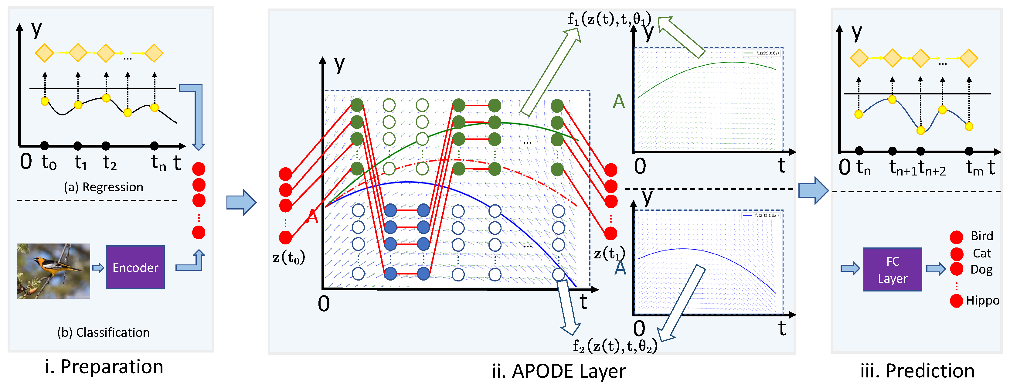
Figure 3.
(a) An example path of APODE from to where indicates a certain time step; (b) APODE can be regarded as a model composed of multiple candidate paths during training.
Figure 3.
(a) An example path of APODE from to where indicates a certain time step; (b) APODE can be regarded as a model composed of multiple candidate paths during training.
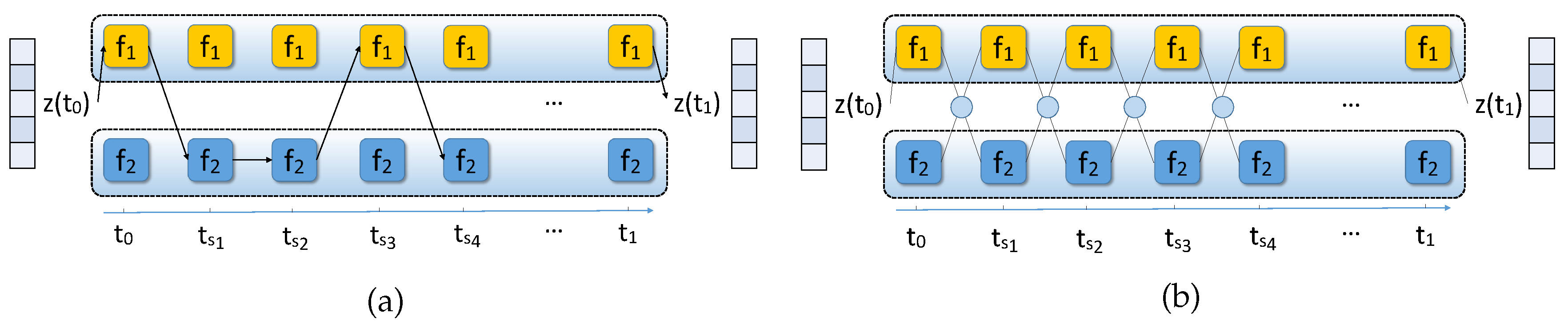
Figure 4.
(a) An inherent limitation of an ODE is that continuous trajectories mapping from -1 to 1 (represented by blue) and from 1 to -1 (represented by green) cannot intersect each other; (b) The hidden representation starting from is not absolutely sandwiched between those two starting from and of APODE. Note that this figure characterizes the hidden representations of different initial values in APODE, which should be distinguished from Figure 1(b) of the same initial value.
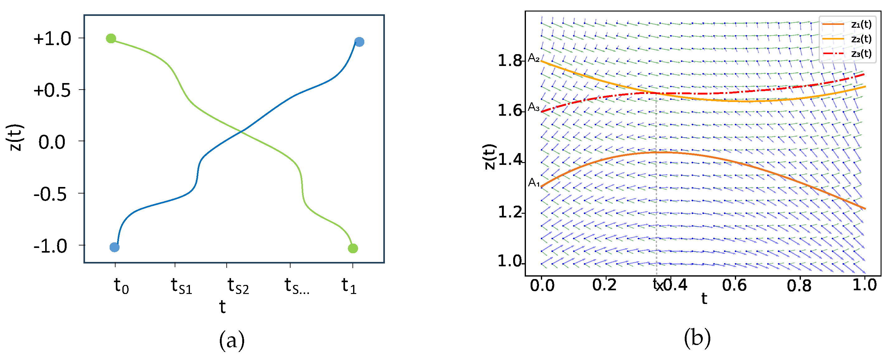
Figure 5.
Diagram of the sphere dataset: (left) for ; (right) for .
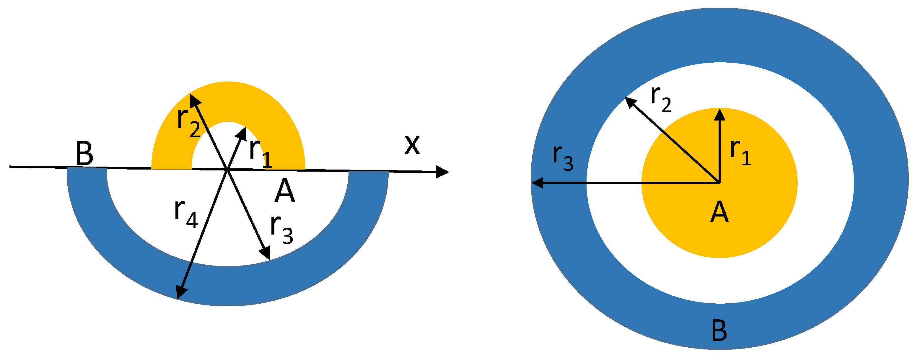
Figure 6.
Comparison of APODE and vanilla NODE on the sphere dataset: (left) for ; (right) for .
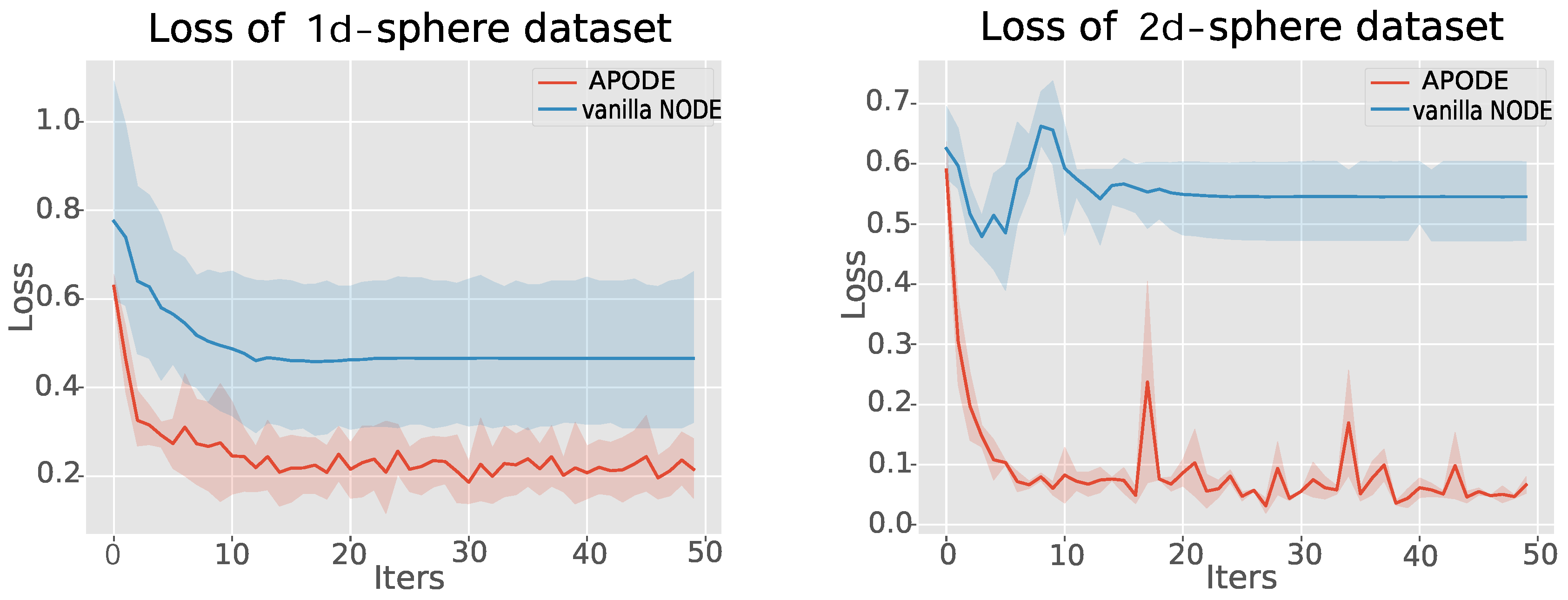
Figure 7.
(a) Classification accuracies of APODE under different settings of p, which varies from 0 to 1; (b) Classification accuracies and standard deviations of APODE and Ensemble on Cifar10, SVHN, Cifar100 and F-mnist.
Figure 7.
(a) Classification accuracies of APODE under different settings of p, which varies from 0 to 1; (b) Classification accuracies and standard deviations of APODE and Ensemble on Cifar10, SVHN, Cifar100 and F-mnist.
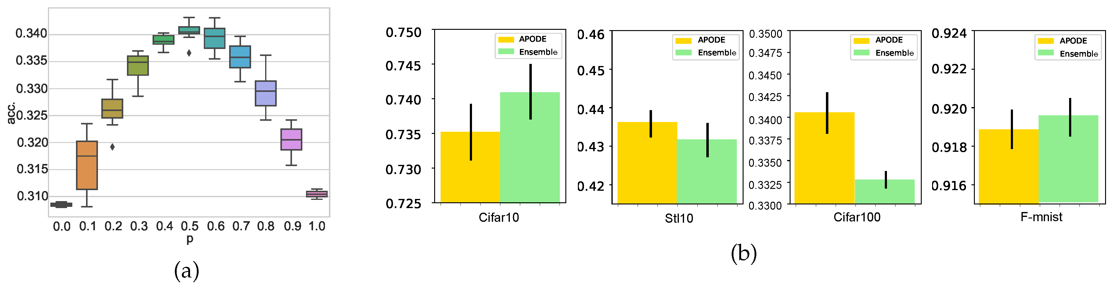
Figure 8.
The qualitative behaviour of periodic trajectories on Latent ODE vs. Latent ODE+APODE. The six columns correspond to various sampling data on Latent ODE and Latent ODE+APODE, respectively.
Figure 8.
The qualitative behaviour of periodic trajectories on Latent ODE vs. Latent ODE+APODE. The six columns correspond to various sampling data on Latent ODE and Latent ODE+APODE, respectively.
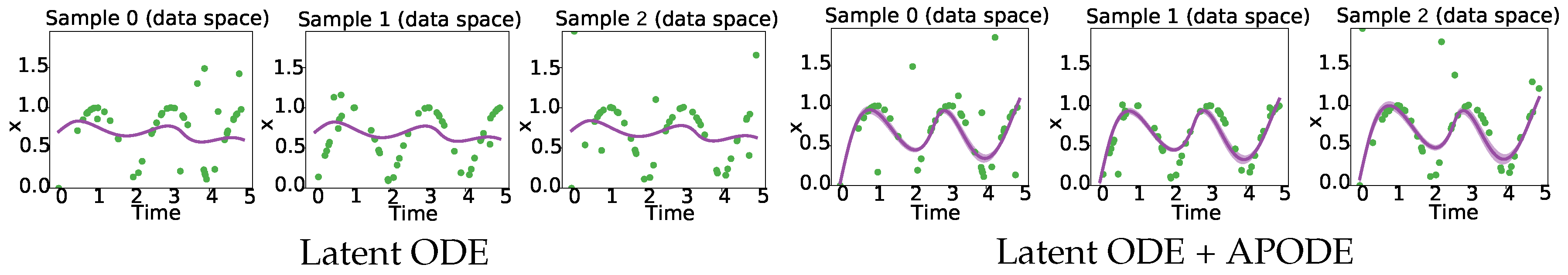
Table 2.
Experimental results on MNIST compared with different adversarial attacks. ARC is not applicable to vanilla NODEs.
Table 2.
Experimental results on MNIST compared with different adversarial attacks. ARC is not applicable to vanilla NODEs.
| PGD | ARC | |
| NODE | 64.7 | - |
| APODE* | 78.0 | 68.4 |
Disclaimer/Publisher’s Note: The statements, opinions and data contained in all publications are solely those of the individual author(s) and contributor(s) and not of MDPI and/or the editor(s). MDPI and/or the editor(s) disclaim responsibility for any injury to people or property resulting from any ideas, methods, instructions or products referred to in the content. |
© 2025 by the authors. Licensee MDPI, Basel, Switzerland. This article is an open access article distributed under the terms and conditions of the Creative Commons Attribution (CC BY) license (http://creativecommons.org/licenses/by/4.0/).
Copyright: This open access article is published under a Creative Commons CC BY 4.0 license, which permit the free download, distribution, and reuse, provided that the author and preprint are cited in any reuse.


