Submitted:
27 May 2025
Posted:
28 May 2025
You are already at the latest version
Abstract
Large-scale heating, ventilation, and air conditioning (HVAC) control systems in pharmaceutical manufacturing are characterized by numerous operational parame-ters, delayed fault detection, and challenges in fault diagnosis. This study proposes a data-driven early warning method for equipment parameters, integrating Principal Component Analysis (PCA) and Nonlinear State Estimation Technology (NSET). Ini-tially, operational data collected from air conditioning units are preprocessed and an-alyzed to extract parameters relevant to fault detection. A nonlinear state estimation predictive model is constructed by minimizing the residuals, and its performance is further optimized using PCA. Actual operational data from the SCADA system are then utilized to predict and analyze deviations in the mixed-room temperature during production. Fault detection is achieved by evaluating whether the prediction residuals exceed a predefined critical threshold, allowing for timely identification of abnormal operating conditions. Comparative analysis of system data before and after faults is conducted to further validate the approach. Experimental results demonstrate that the proposed PCA-NSET model is feasible and effective for fault detection in HVAC con-trol systems within pharmaceutical workshops.
Keywords:
fault detection
; nonlinear state estimation
; principal component analysis
; SCADA
; pharmaceutical manufacturing
1. Introduction
In pharmaceutical manufacturing, the environmental conditions of production workshops—including temperature, humidity, cleanliness, and pressure differentials—directly affect the quality and safety of pharmaceutical products [1,2]. Different types of pharmaceuticals impose distinct requirements on these environmental parameters. To ensure that production environments meet stringent regulatory standards, it is essential to employ reliable HVAC (heating, ventilation, and air conditioning) control systems to regulate the operation of all critical equipment [3]. Consequently, the adoption of effective monitoring and fault diagnosis techniques is of great significance for maintaining high product quality and production yield.
The HVAC control system in pharmaceutical workshops typically adjusts chilled water valves, hot water valves, humidification valves, and other equipment to maintain air parameters (e.g., temperature, humidity, and pressure) at their setpoints [4]. Compared to physical-model-based or empirical-model-based methods, data-driven models offer the advantages of not requiring detailed knowledge of system structure and exhibiting superior generalization capability [5,6]. Modern HVAC systems are often equipped with SCADA (Supervisory Control and Data Acquisition) platforms, which integrate extensive sensor networks to collect and archive large volumes of operational data. Proper utilization of these data enables the monitoring of equipment states, and data-driven state variable models constructed from historical data under normal operating conditions can facilitate fault detection by analyzing the residuals between predicted and measured values [7].
Artificial neural networks, particularly those employing backpropagation algorithms, have been widely applied in the fault detection and diagnosis of HVAC systems and related equipment [8]. Some studies have integrated backpropagation neural networks with decision tree methods to enhance the detection and classification of both known and unknown faults [9,10]. The introduction of algorithms such as Round Robin Dithering (RDP) has further simplified neural network models for fault diagnosis, improving diagnostic efficiency without sacrificing accuracy [11]. While neural networks possess powerful learning capabilities [8], their diagnostic performance heavily depends on the quality and quantity of training data, and the resulting models often lack interpretability and extensibility, limiting their practical application.
Nonlinear State Estimation Technology (NSET), originally proposed by Singer et al. [9], is a data-driven, nonparametric, and nonlinear empirical modeling method. It has been successfully applied to early fault warning in wind turbine generators [10], and further improvements have been achieved by integrating additional fault detection algorithms to enhance prediction accuracy [11]. However, the effectiveness of NSET relies on the selection of a representative process memory matrix constructed from historical data. This approach has notable limitations: (i) expert-selected samples may lack representativeness, and (ii) selecting too many historical samples can result in an excessively large memory matrix [12].
To address these challenges, this work proposes an integrated approach combining Principal Component Analysis (PCA) with NSET [13]. The main idea is to utilize PCA for data cleaning and dimensionality reduction of SCADA-acquired datasets, thereby constructing a temperature prediction model for the HVAC system under normal operation [14]. This enables real-time and accurate fault diagnosis, facilitating the timely identification of potential failures and the implementation of preventive maintenance strategies to ensure the reliable and safe operation of the system.
2. Materials and Methods
2.1. Data Preprocessing
When the number of measurements is sufficiently large, it can be assumed that the sample data follow a normal distribution [15]. Assuming the data contain only random errors, the standard deviation of the dataset can be calculated to define a confidence interval. Any measurement error that falls outside this interval is considered a gross error, which can be identified as an outlier or abnormal data point [16].
Let a set of measurements be denoted as, The mean and deviation of the dataset are calculated. If, for a particular data point , the deviation satisfies the following condition:
then the data pointis considered to be an outlier.
Prior to further processing, the raw data should be normalized to eliminate the influence of different units and scales [17]. Z-score normalization is a commonly used method for standardizing data. This approach standardizes the original data based on its mean and standard deviation, which alters the scale of the data but does not change the type of its distribution [18]. Z-score normalization is particularly suitable for situations where the maximum and minimum values of the dataset are unknown.
In Equation (2),denotes the standardized data,represents the mean of the sample data, andis the standard deviation of the sample data. After standardization, the processed data follow a distribution with a mean of 0 and a standard deviation of 1.
2.2. Feature Selection and Principal Component Analysis
The object of this study is the HVAC system of a pharmaceutical manufacturing facility located in Zhejiang Province, China. This system controls three separate rooms: the weighing room (w-room) for measuring raw materials, the preprocessing room (p-room) for preliminary handling of ingredients, and the mixing room (m-room) for final product manufacturing. To develop the NSET model for temperature prediction in the mixing room, it is necessary to identify the parameters in the SCADA system that are most closely related to the mixing room temperature [18,19]. The parameters recorded by the SCADA system, along with their Pearson correlation coefficients with the mixing room temperature and their respective operating ranges, are summarized in Table 1.
As shown in Table 1, the mixing room temperature exhibits a strong positive correlation with both the weighing room temperature and the preprocessing room temperature. This is primarily because all three rooms are regulated by the same HVAC system. However, it should be noted that the Pearson correlation coefficient has certain limitations: it is only suitable for describing linear relationships, is sensitive to outliers, and does not provide information about causal relationships [20]. Therefore, it is necessary to combine other methods for more robust and comprehensive variable selection in the modeling process.
Principal Component Analysis (PCA) is a widely used dimensionality reduction algorithm [21,22]. The fundamental idea of PCA is to transform a set of correlated variables into a smaller number of uncorrelated composite variables, known as principal components, through linear combination. These principal components are designed to capture as much of the useful information from the original data as possible [23]. The specific steps for determining the principal components are as follows:
Suppose there areobserved variables, denoted as,. Let the correlation coefficient between variablesandbe. The principal steps for performing PCA are as follows:
1. Data preprocessing. Prepare the raw data for analysis, typically involving normalization or standardization.
2. Calculation of correlation coefficients. Compute the pairwise correlation coefficients among all variables to obtain the correlation coefficient matrix.
3. Eigenvalue and eigenvector computation. Calculate the eigenvalues and corresponding eigenvectorsof the correlation coefficient matrix. The eigenvectors represent the directions of the principal components.
4. Calculation of variance contribution rates. Determine the variance contribution rate of each principal component, as well as the cumulative variance contribution rateof the first principal components.
Principal component analysis was performed on the parameters recorded by the SCADA system using Equation (3). The contribution rates and cumulative contribution rates of all principal component vectors were calculated and then ranked in descending order of their contribution rates, as illustrated in Figure 1.
The variance contribution rates and cumulative variance contribution rates of the principal components for all operating parameters are systematically summarized in Table 2. These values were calculated based on the results of the PCA conducted on the dataset acquired from the SCADA system [25]. As shown, each operating parameter exhibits a distinct contribution to the overall variance, and the cumulative contribution rates demonstrate how much of the total information from the original data is retained as additional components are included. This comprehensive summary provides an essential foundation for subsequent variable selection and model construction in this study.
As shown in Table 2, the cumulative contribution rate of the first six principal components reaches 98.4%. Therefore, selecting the first six principal components ensures that a sufficient amount of the original data’s information is retained while also maintaining high computational efficiency [26].
Based on the above analysis, the variables selected for model construction are as follows: mixing room temperature, preprocessing room temperature, weighing room temperature, supply air duct humidity, mixing room humidity, and fan frequency [25].
The temperature of the air conditioning system is affected by seasonal variations; therefore, the modeling period should not be excessively long. In this study, the model was developed using operational data collected over a three-month period, specifically from 00:50 on December 22, 2023, to 16:20 on March 22, 2024. The dataset consists of 13,198 records, with a sampling interval of 10 minutes.
The variation in the mixing room temperature during this period is illustrated in Figure 2.
As shown in Figure 2, the mixing room temperature is noticeably lower during the period corresponding to data points 6420 to 7676 compared to other times. This is because the air conditioning unit was not in operation during this interval, resulting in the room temperature reflecting the ambient (uncontrolled) conditions. This observation is further supported by the variation in the supply fan frequency of the air conditioning unit, as depicted in Figure 3.
In addition to the non-operational period between data points 6420 and 7676, there are also isolated instances at other times where the supply fan frequency is zero. These data points are considered abnormal and are treated as outliers. Therefore, thorough data preprocessing is required before constructing the temperature prediction model for the air conditioning system [26].
2.3. Nonlinear State Estimation Modeling
In this study, a nonlinear state estimation (NSET) method is employed to develop a temperature prediction model for the air conditioning system under normal operating conditions [27,28]. The established model is then used to predict the system’s output, and the residuals—defined as the differences between the measured and predicted values—are analyzed. The magnitude, range, and variation of these residuals provide important information for assessing the operational status of the HVAC unit [29]. When the system experiences an abnormal condition, its dynamic characteristics deviate from those observed during normal operation, resulting in increased residuals. This forms the basis for early fault detection and warning for the air conditioning unit or related equipment.
At a specific time, the air conditioning unit collectsinterrelated variables, which are represented as an observation vector [30].
The system observation matrixcan thus be expressed as follows:
In Equation (5),denotes the number of observation vectors, andrepresents the number of variables in each observation vector.
The process memory matrixserves as a memory and representation of the system’s normal operating conditions [31]. It is constructed by selectingobservation vectors under different normal operating scenarios.
Each column of the process memory matrixrepresents an observation vector corresponding to a specific normal operating condition of the system. Therefore, it is essential to carefully select the data before constructing the matrix, ensuring that thehistorical observation vectors used inadequately represent the full range of normal operating scenarios [32]. Ideally, the process memory matrixshould encompass all typical normal operating states of the air conditioning system.
The input to the NSET model is an observation vectorat a given time, and the output is the corresponding predicted vector. For any input observation vector, the NSET model generates a-dimensional weight vector [33]. The vector is a column vector whose dimension is equal to the number of components in the input observation vector.
The predicted vectorcan be expressed as follows:
The weight vector is obtained by minimizing the residual between the predicted vectorand the observation vector[34]:
In Equation (9),denotes a nonlinear operator. There are various choices for the nonlinear operator; in this study, the Euclidean distance betweenandis used, as follows:
By substituting Equation (9) into Equation (8), the prediction vector of the NSET model can be obtained as follows:
Using Equation (11), the predicted value of the current input data can be obtained from historical data, which ultimately provides diagnostic information regarding potential faults in the system [37].
3. Results and Discussion
3.1. Data Preprocessing Effects
The NSET model prediction residual for the mixing room temperature is given by [35]:
In Equation (11), represents the mixing room temperature component in the input observation vector for the NSET model, while denotes the corresponding predicted value of the mixing room temperature. In the training set, the residuals of the NSET models for the mixing room temperature are compared for both the raw (unprocessed) data and the preprocessed data. The comparison results are shown in Figure 4.
As shown in Figure 4, except for a few time points, the residuals of the mixing room temperature predicted by the model built with preprocessed data are generally smaller than those obtained with unprocessed data. This demonstrates that data preprocessing is both necessary and effective for improving the model’s prediction accuracy.
3.2. Model Comparison and Fault Detection Performance
Experimental data from one week in March were selected to evaluate the performance of the air conditioning control system models [36,37]. A comparison between the conventional NSET model and the proposed PCA-NSET model clearly demonstrates the superior accuracy of the latter, as illustrated in Figure 5. As shown, the residuals and error fluctuations of the PCA-NSET model are significantly smaller than those of the conventional NSET model, indicating that the PCA-NSET model achieves higher prediction accuracy and better overall performance.
Experimental validation was conducted using data from March 14 to March 22. During this eight-day period, the air conditioning unit operated normally for the first seven days, while a fault occurred on the eighth day. The established PCA-NSET model was applied to perform fault analysis on this dataset. The threshold for residuals can be determined either empirically by the operators or based on the Laida criterion described in Section 2.1. The predicted mixing room temperature and the corresponding temperature residuals for both the first seven days and the eighth day are shown in Figure 6 and Figure 7, respectively.
As shown in Figure 6, when the air conditioning control system is operating normally, the model’s predicted values closely match the observed values, with residuals remaining within the threshold except for a few isolated points. In contrast, Figure 7 demonstrates that when a fault occurs in the system, there is a significant deviation between the predicted and observed values. The residuals rapidly increase and consistently exceed the threshold within a short period. Therefore, by monitoring the residuals, effective fault prediction can be achieved; specifically, frequent exceedance of the threshold by the residuals can serve as an early warning indicator for system faults.
4. Conclusions
This study investigates the operational status and fault detection of air conditioning units based on SCADA monitoring data. After performing data preprocessing, a predictive model was developed using a combination of Principal Component Analysis (PCA) and Nonlinear State Estimation Technology (NSET), and its performance was compared with that of the conventional NSET model. The results demonstrate that the PCA-NSET model achieves higher accuracy than the conventional NSET model, verifying the effectiveness of the proposed approach. Further analysis of the SCADA data from the air conditioning unit shows that, under normal operating conditions, the model’s residuals remain within a reasonable range, whereas during a fault, the residuals consistently exceed the threshold. Experimental results confirm that the proposed PCA-NSET model provides excellent performance in detecting faults in air conditioning control systems.
Author Contributions
Daiyuan Huang was responsible for the conceptualization of the study, algorithm development, experimental design, data curation, and conducting the experimental analysis. Daiyuan Huang also drafted the original manuscript and performed the visualization of results. Wenjun Yan provided theoretical supervision, offered guidance on the research direction, and contributed to the review and editing of the manuscript. Both authors contributed to the discussion and interpretation of results. All authors have read and agreed to the published version of the manuscript.
Funding
This research received no funding
Data Availability Statement
The data that support the findings of this study are available from the authors upon reasonable request. Requests for data can be made by contacting the corresponding author via email.
Acknowledgments
The authors would like to thank Zhejiang Lepu Pharmaceutical Co., Ltd. for providing the experimental data used in this study. During the preparation of this manuscript, the authors used ChatGPT to assist with language editing and manuscript polishing. The authors have reviewed and edited the output and take full responsibility for the content of this publication.
Conflicts of Interest
The authors declare no conflicts of interest.
References
- Qin, S. Joe. Survey on data-driven industrial process monitoring and diagnosis. Annual Reviews in Control 36.2 (2012): 220-234. [CrossRef]
- Chiang, L.H., Russell, E.L., & Braatz, R.D. Fault diagnosis in chemical processes using Fisher discriminant analysis, discriminant partial least squares, and principal component analysis. Chemometrics and Intelligent Laboratory Systems 50.2 (2000): 243-252. [CrossRef]
- Wang, Shiyu, & Qin, S. Joe. A new subspace identification approach for modeling and control of HVAC systems. Control Engineering Practice 16.7 (2008): 796-808. [CrossRef]
- Li, Wei, et al. Data-driven HVAC system modeling and prediction: A review. Energy and Buildings 209 (2020): 109656. [CrossRef]
- Zhao, Bin, et al. “A review on fault detection and diagnosis for HVAC systems.” Energy and Buildings 72 (2014): 154-162. [CrossRef]
- Yin, Shoubin, et al. “A review on advances in data-driven fault detection and diagnosis for building energy systems.” Energy and Buildings 248 (2021): 111174. [CrossRef]
- Venkatasubramanian, V., et al. “A review of process fault detection and diagnosis: Part I: Quantitative model-based methods.” Computers & Chemical Engineering 27.3 (2003): 293-311. [CrossRef]
- Alcala, C.F., & Qin, S. Joe. “Detection and diagnosis of process faults based on principal component analysis.” Journal of Process Control 19.10 (2009): 1793-1803.
- Russell, E.L., Chiang, L.H., & Braatz, R.D. “Data-driven techniques for fault detection and diagnosis in chemical processes.” Springer Science & Business Media, 2012. [CrossRef]
- Qin, S. Joe. “Statistical process monitoring: basics and beyond.” Journal of Chemometrics 17.8-9 (2003): 480-502. [CrossRef]
- Feng, X., et al. “A practical approach for model-based fault detection and diagnosis in HVAC systems.” Energy and Buildings 216 (2020): 109942. [CrossRef]
- Zhao, Y., et al. “Review on data-driven modeling and optimization for building energy systems.” Renewable and Sustainable Energy Reviews 137 (2021): 110591. [CrossRef]
- Zhu, Y., & He, S. “Fault detection and diagnosis for building air handling units using machine learning and expert knowledge.” Energy and Buildings 219 (2020): 110007. [CrossRef]
- Shao, Xiang, et al. “A data-driven approach for fault detection and diagnosis in building HVAC systems.” Energy and Buildings 218 (2020): 110018. [CrossRef]
- Yu, H., & Qin, S. Joe. “Multivariate statistical monitoring using dynamic principal component analysis.” Industrial & Engineering Chemistry Research 40.15 (2001): 3382-3401.
- Shang, Chuanbo, & You, Qingchun. “A hybrid intelligent method for fault detection and diagnosis of HVAC systems based on PCA and Fuzzy ARTMAP neural network.” Building and Environment 196 (2021): 107792. [CrossRef]
- Venkatasubramanian, V. “Process fault detection and diagnosis: past, present and future.” Computers & Chemical Engineering 27.3 (2003): 293-311. [CrossRef]
- Li, J., et al. “Nonlinear state estimation technique for wind turbine condition monitoring and fault diagnosis.” Renewable Energy 138 (2019): 636-648. [CrossRef]
- Li, Yan, et al. “Review of building energy modeling for control and operation.” Renewable and Sustainable Energy Reviews 137 (2021): 110608. [CrossRef]
- Wang, Wei, et al. “A survey on data-driven fault detection and diagnosis for HVAC systems.” Energy and Buildings 225 (2020): 110322. [CrossRef]
- Xie, Li, et al. “Nonlinear state estimation for process monitoring and fault diagnosis: A review.” Journal of Process Control 87 (2020): 13-27. [CrossRef]
- Liu, X., et al. “Data-driven techniques in fault detection and diagnosis for HVAC systems: A review.” Applied Energy 272 (2020): 115127. [CrossRef]
- Ma, Y., et al. “Model predictive control for the operation of building cooling systems: Review and future opportunities.” Applied Energy 179 (2016): 47-61. [CrossRef]
- Zhou, S., et al. “A survey of data-driven building fault detection and diagnosis.” Energy and Buildings 203 (2019): 109434. [CrossRef]
- Wang, S., & Xiao, F. “A review on model predictive control for buildings.” Building and Environment 105 (2016): 301-312. [CrossRef]
- Ding, Steven X., et al. “Data-driven design of fault diagnosis and fault-tolerant control systems.” Annual Reviews in Control 44 (2017): 84-105. [CrossRef]
- Li, Haibo, et al. “A hybrid PCA-based fault detection approach for building HVAC systems.” Energy and Buildings 141 (2017): 182-193. [CrossRef]
- Zhao, X., et al. “Data-driven fault detection for industrial processes based on stacked autoencoder and feature learning.” Industrial & Engineering Chemistry Research 59.30 (2020): 13471-13483.
- Sun, X., et al. “Dynamic principal component analysis for process monitoring and fault diagnosis: A review.” Industrial & Engineering Chemistry Research 58.34 (2019): 15506-15519.
- MacGregor, J.F., & Kourti, T. “Statistical process control of multivariate processes.” Control Engineering Practice 3.3 (1995): 403-414. [CrossRef]
- He, S., et al. “Nonlinear process monitoring based on kernel principal component analysis.” Chemical Engineering Science 56.2 (2001): 579-590.
- Kano, M., & Nakagawa, Y. “Data-based process monitoring, process control, and quality improvement: Recent developments and applications in chemical process industries.” Computers & Chemical Engineering 45 (2012): 104-116. [CrossRef]
- Venkatasubramanian, V. “A review of process fault detection and diagnosis: Part II: Qualitative models and search strategies.” Computers & Chemical Engineering 27.3 (2003): 313-326. [CrossRef]
- Qin, S. Joe. “Data-driven fault detection and process monitoring for complex chemical processes.” AIChE Journal 67.6 (2021): e17211. [CrossRef]
- Li, J., Li, Q., & Zhou, J. “A review of artificial intelligence methods for data-driven fault detection and diagnosis in building HVAC systems.” Energy and Buildings 246 (2021): 111073. [CrossRef]
- Shao, Y., et al. “A novel data-driven method for building fault detection and diagnosis using improved principal component analysis and random forest.” Energy and Buildings 208 (2020): 109624. [CrossRef]
- Lin, Y., et al. “Fault detection and diagnosis for building air handling units using supervised machine learning and expert rules.” Applied Energy 254 (2019): 113673. [CrossRef]
- Yu, J., et al. “A review of data-driven methods for HVAC system fault detection and diagnosis.” Energy and Buildings 212 (2020): 109807. [CrossRef]
- Chiang, Leo H., et al. “Fault detection and diagnosis in industrial systems.” Springer, 2017.
- Yan, C., O’Brien, W., & Gunay, B. “A comprehensive review of monitoring-based commissioning: Recurrent faults, energy impacts, and future research needs.” Energy and Buildings 186 (2019): 84-100. [CrossRef]
Figure 1.
Cumulative variance contribution rates of the principal components derived from SCADA system parameters.
Figure 1.
Cumulative variance contribution rates of the principal components derived from SCADA system parameters.
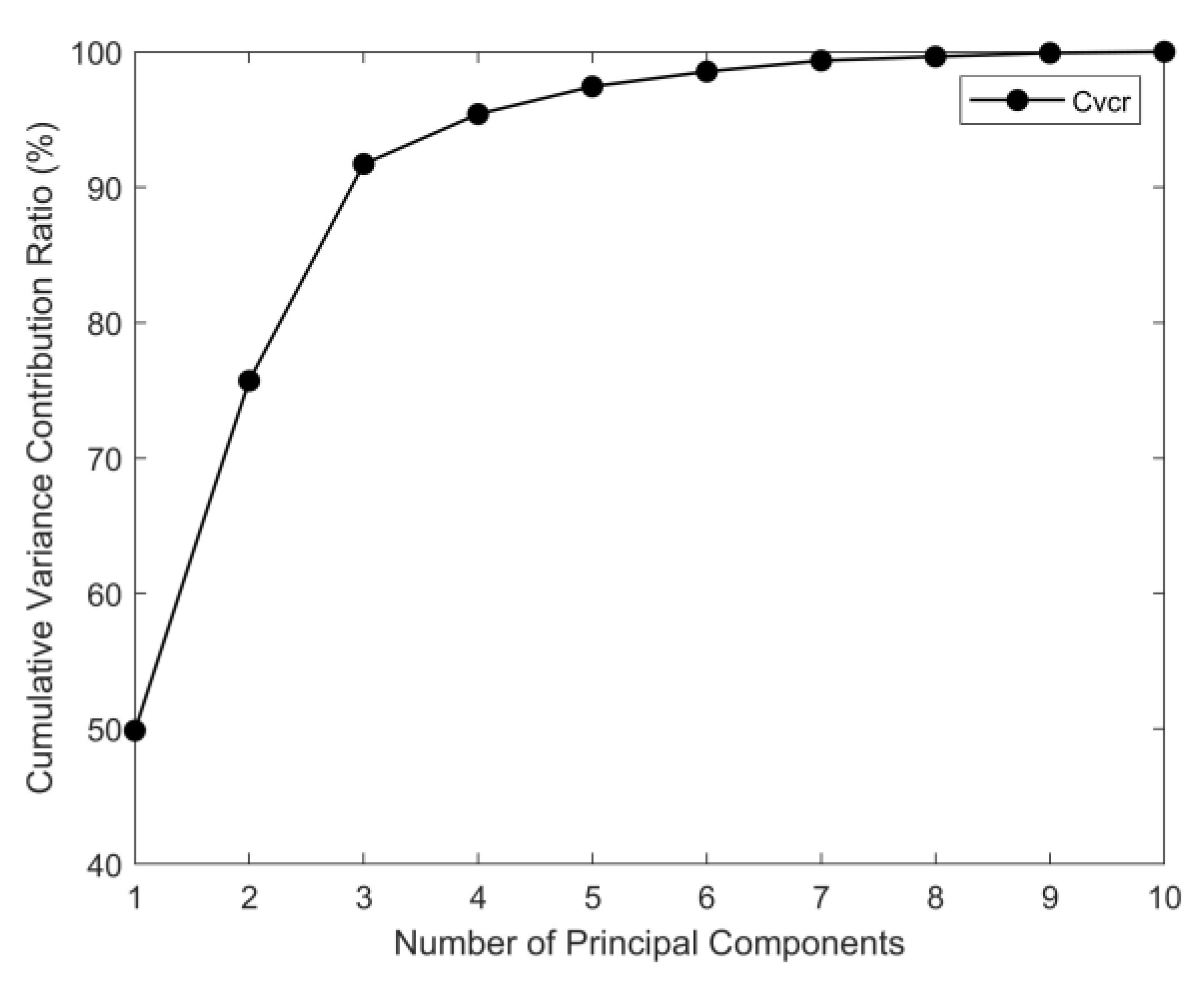
Figure 2.
Temperature variation curve of the mixing room during the study period.
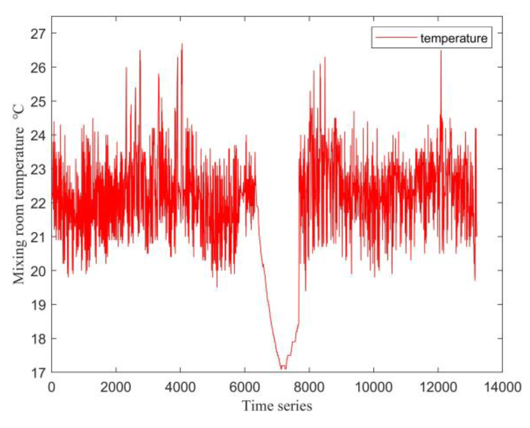
Figure 3.
Variation curve of the supply fan frequency during the study period.
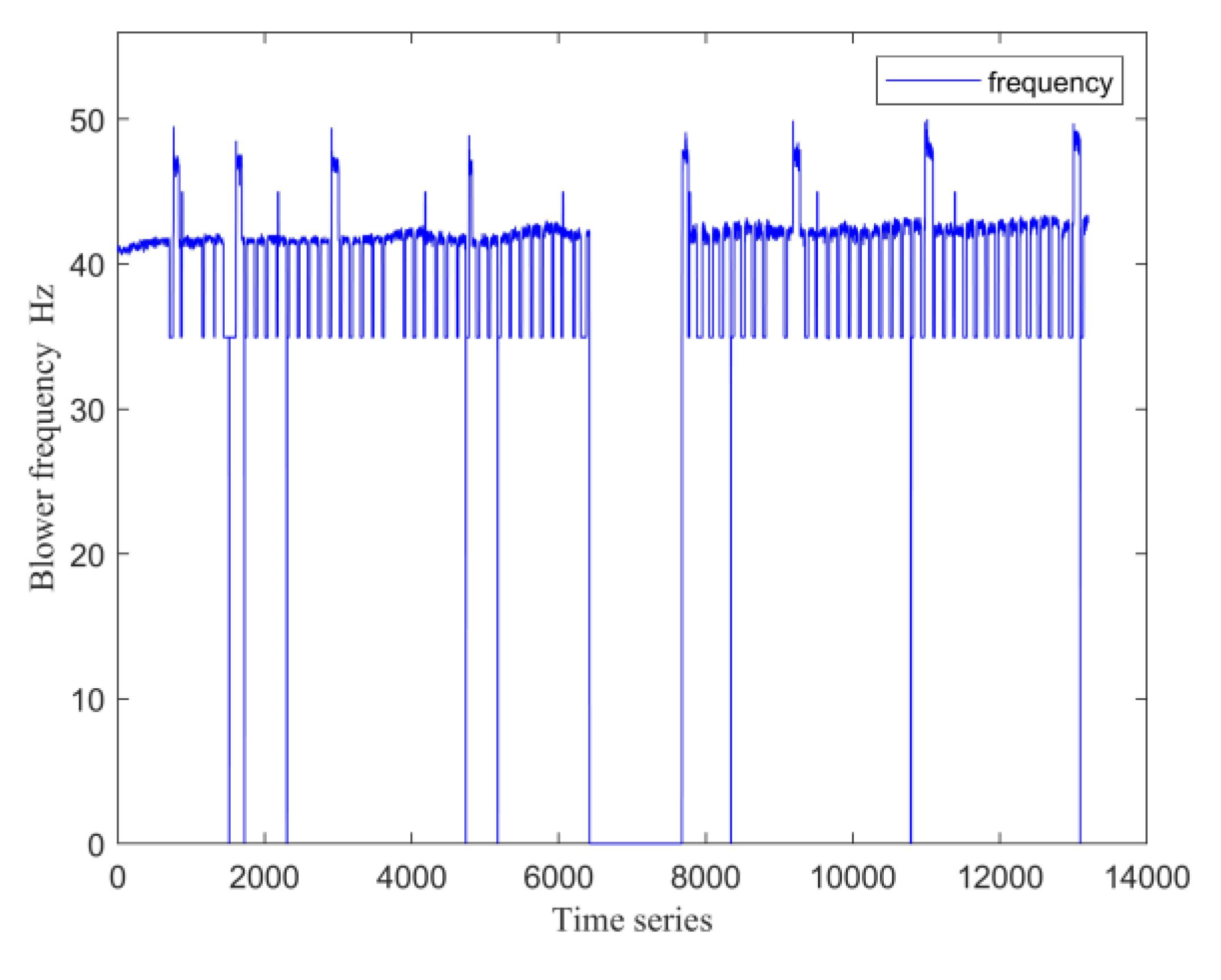
Figure 4.
Variation curves of residuals before and after data preprocessing.
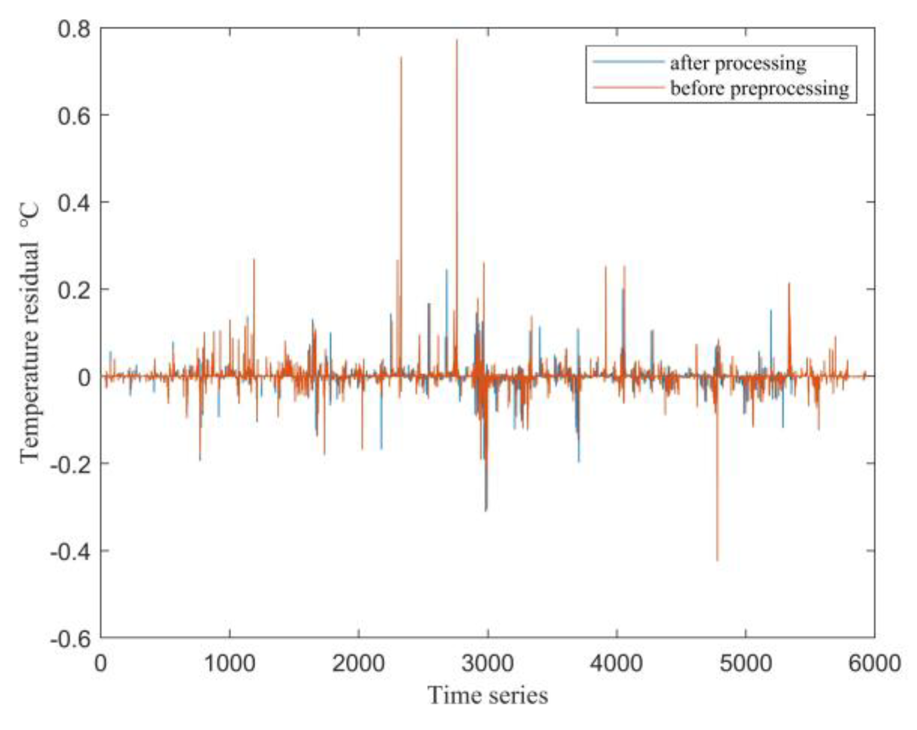
Figure 5.
Comparison of residuals between the conventional NSET model and the proposed PCA-NSET model.
Figure 5.
Comparison of residuals between the conventional NSET model and the proposed PCA-NSET model.
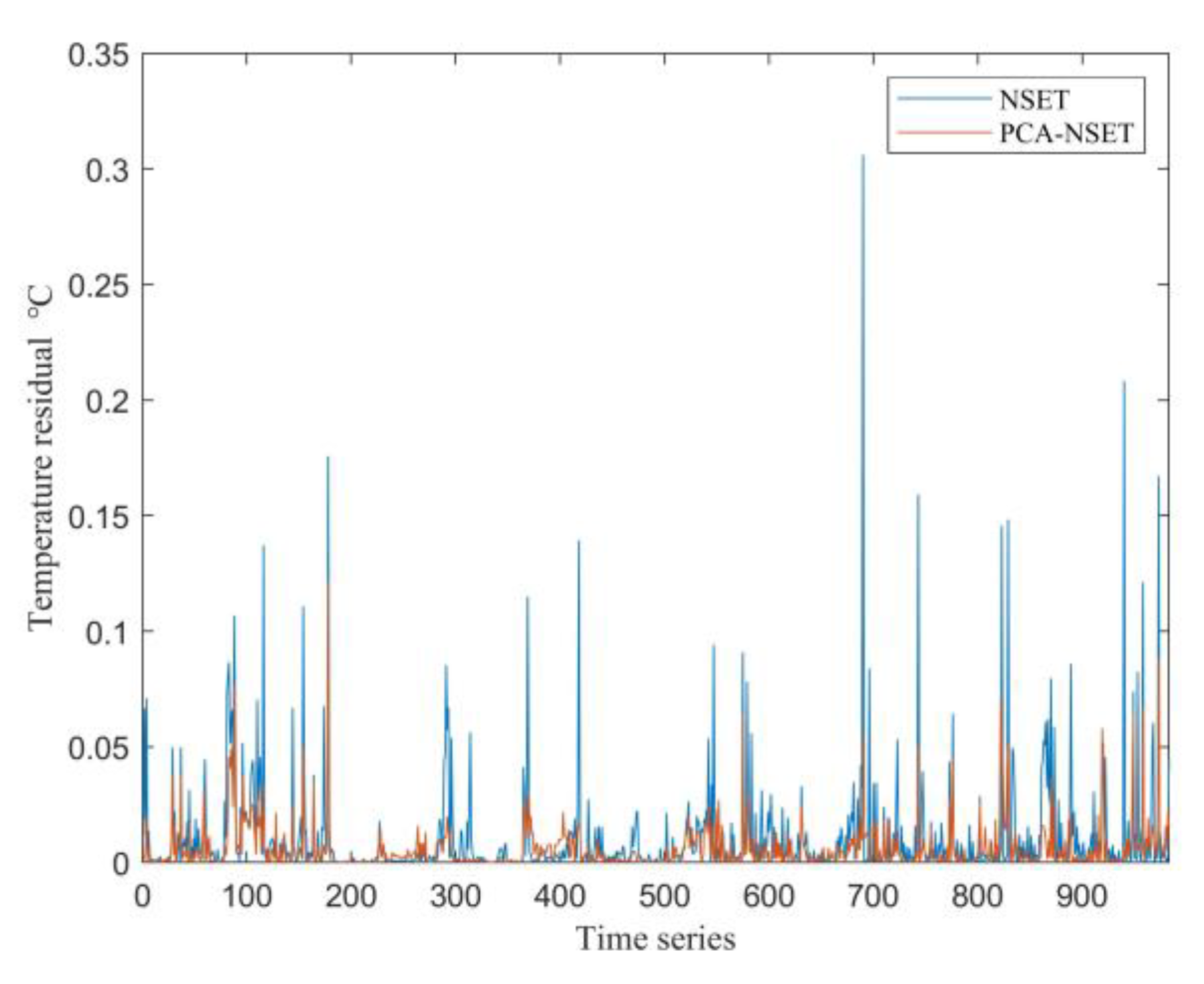
Figure 6.
Predicted mixing room temperature and residuals during the first seven days of operation: (a) Predicted and actual mixing room temperatures; (b) Residuals of the predicted mixing room temperature.
Figure 6.
Predicted mixing room temperature and residuals during the first seven days of operation: (a) Predicted and actual mixing room temperatures; (b) Residuals of the predicted mixing room temperature.
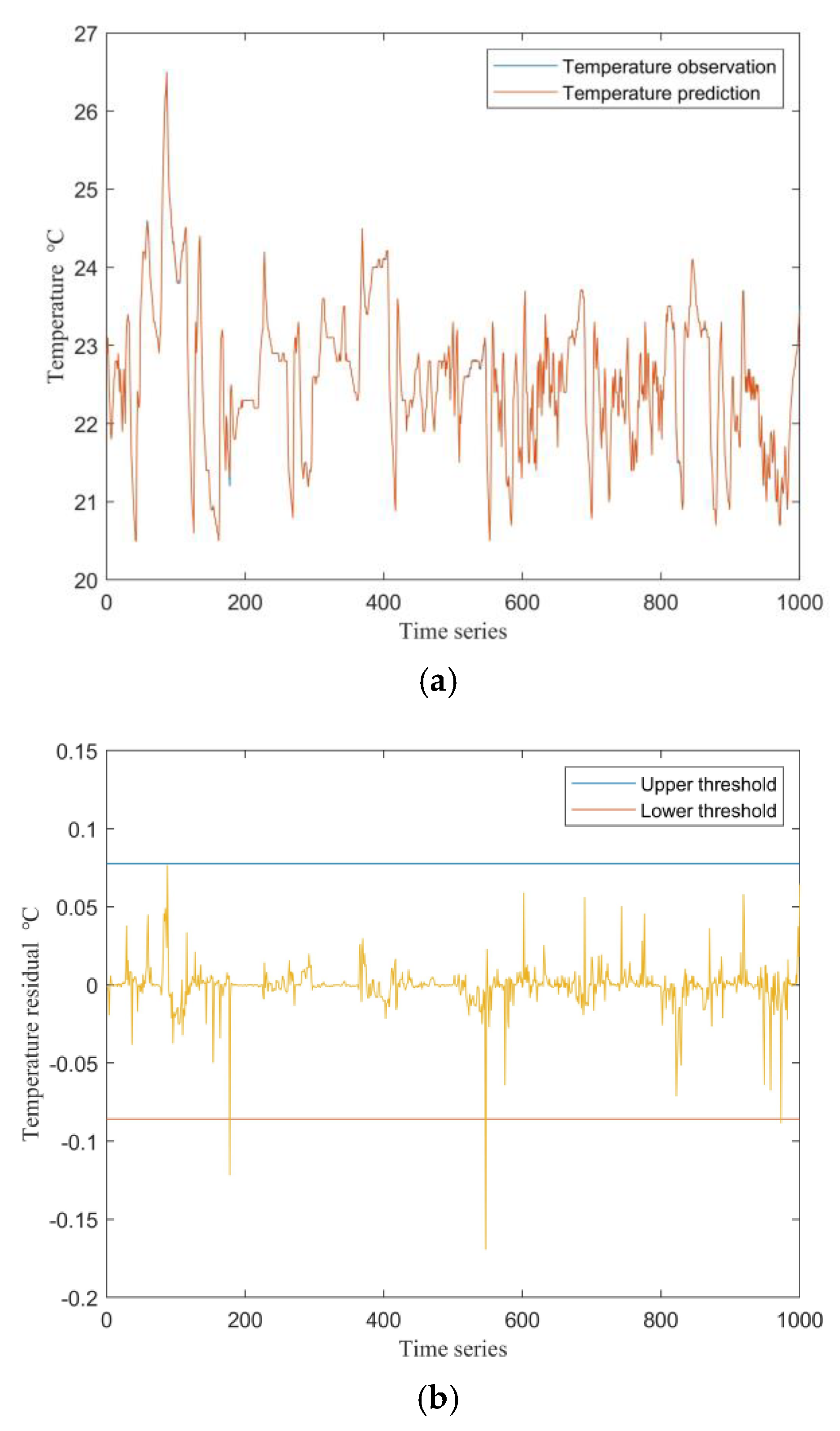
Figure 7.
Predicted mixing room temperature and residuals on the eighth day of operation: (a) Predicted and actual mixing room temperatures; (b) Residuals of the predicted mixing room temperature.
Figure 7.
Predicted mixing room temperature and residuals on the eighth day of operation: (a) Predicted and actual mixing room temperatures; (b) Residuals of the predicted mixing room temperature.
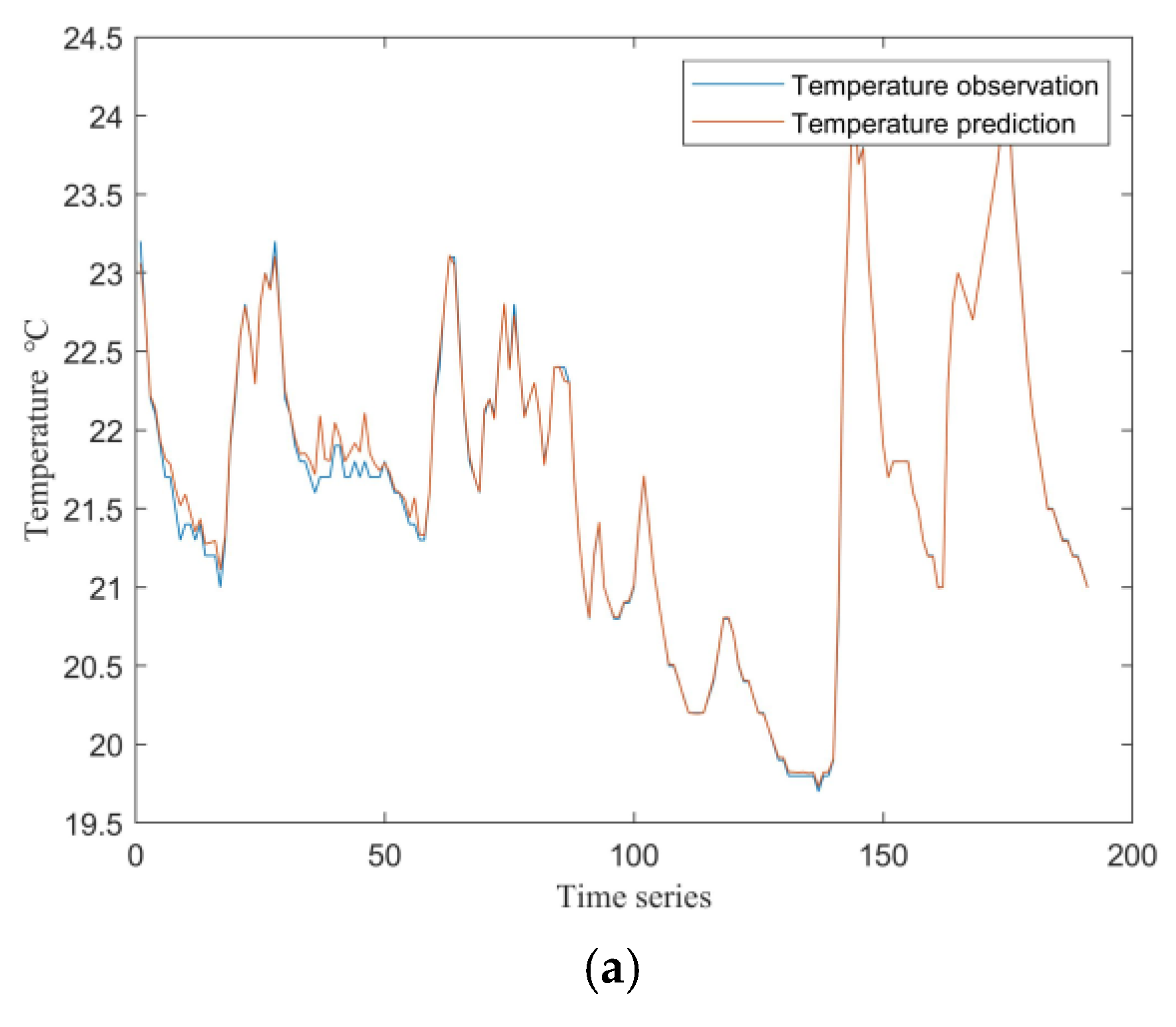
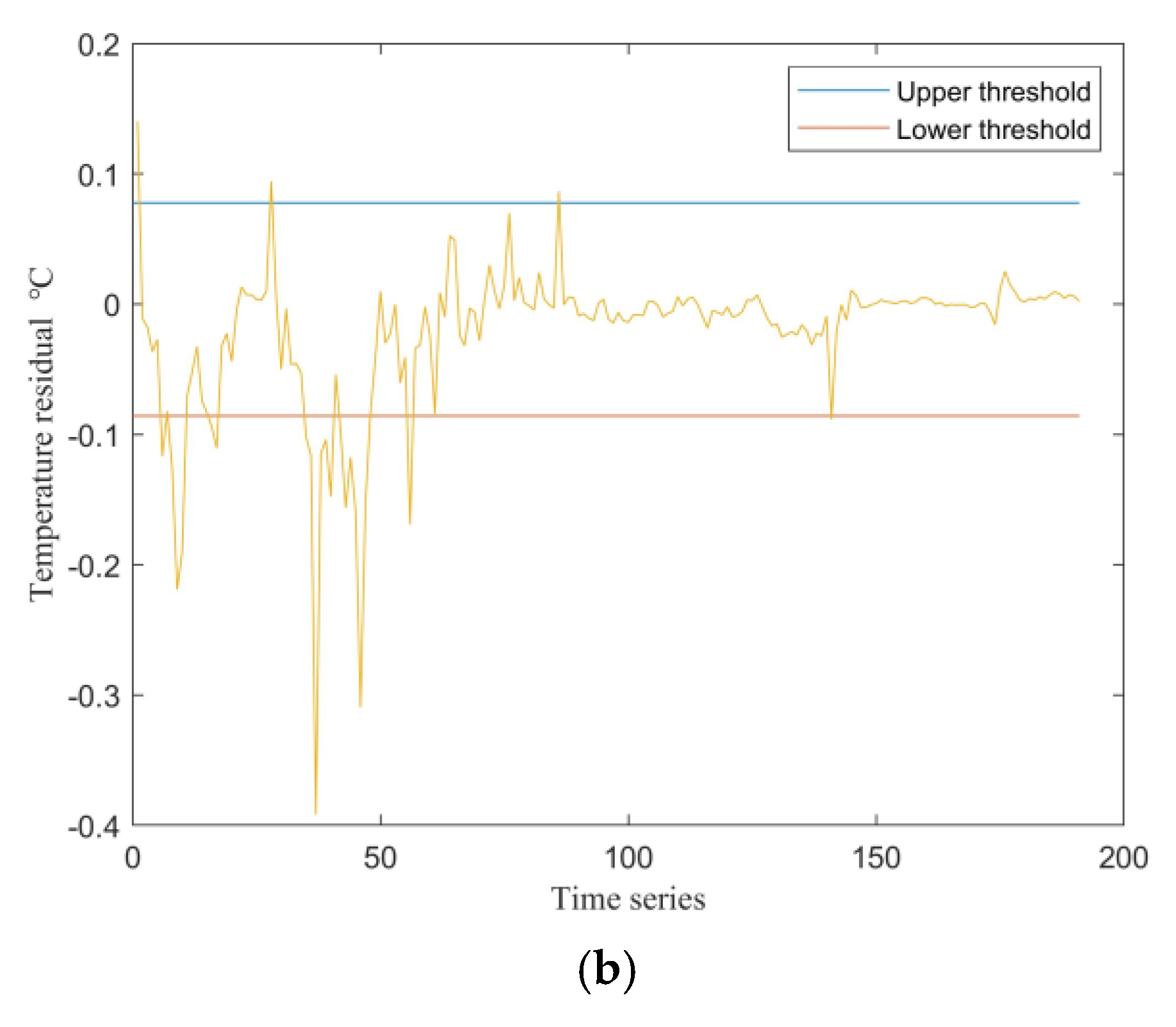

Table 1.
Operating parameter ranges and correlation analysis with mixing room temperature.
| Parameter | Operating Range | Pearson Correlation Coefficient |
| Supply air duct humidity | [13.4,73.2] | -0.280 |
| Supply air duct flow rate | [4912,11687] | -0.167 |
| Fan frequency | [34.8,50] | -0.181 |
| Workshop air flow rate | [57.5,22268] | -0.146 |
| Mixing room temperature | [18.8,26.7] | 1 |
| Mixing room humidity | [21,68.1] | -0.191 |
| Weighing room temperature | [18.8,25.7] | 0.831 |
| Weighing room humidity | [22.1,71.9] | -0.108 |
| Preprocessing room temperature | [19,26.4] | 0.900 |
| Preprocessing room humidity | [21.8,70.6] | -0.280 |
All temperature values are in °C, humidity in %RH, flow rate in m³/h, frequency in Hz.
Table 2.
Principal component variance contribution rates.
| Operating Parameter | Variance Contribution Rate | Cumulative Contribution Rate |
| Mixing room temperature | 0.4986 | 0.4986 |
| Preprocessing room temperature | 0.2584 | 0.757 |
| Weighing room temperature | 0.1601 | 0.9171 |
| Supply air duct humidity | 0.0368 | 0.9536 |
| Mixing room humidity | 0.0204 | 0.974 |
| Fan frequency | 0.0110 | 0.984 |
| Supply air duct flow rate | 0.0081 | 0.9921 |
| Preprocessing room humidity | 0.0029 | 0.995 |
| Workshop air flow rate | 0.0030 | 0.998 |
| Weighing room humidity | 0.0020 | 1 |
PCA was performed on the SCADA system data to obtain the contribution rates.
Disclaimer/Publisher’s Note: The statements, opinions and data contained in all publications are solely those of the individual author(s) and contributor(s) and not of MDPI and/or the editor(s). MDPI and/or the editor(s) disclaim responsibility for any injury to people or property resulting from any ideas, methods, instructions or products referred to in the content. |
© 2025 by the authors. Licensee MDPI, Basel, Switzerland. This article is an open access article distributed under the terms and conditions of the Creative Commons Attribution (CC BY) license (http://creativecommons.org/licenses/by/4.0/).
Copyright: This open access article is published under a Creative Commons CC BY 4.0 license, which permit the free download, distribution, and reuse, provided that the author and preprint are cited in any reuse.


