Submitted:
13 May 2025
Posted:
26 May 2025
You are already at the latest version
Abstract
In this paper, we investigate a class of fuzzy partially differentiable models for Caputo-Hadamard type Goursat problems with generalized Hukuhara (gH) derivatives, which have been widely recognized as having a significant role for simulating and analyzing various kinds of processes in engineering and physical sciences. By transforming an equivalent integral equation and employing classical Banach and Schauder fixed-point theorems, we establish existence and uniqueness of solution for the fuzzy partially differentiable models, respectively. Furthermore, in order to overcome complexity for obtaining exact solutions of systems involving Caputo-Hadamard fractional derivatives, we explore numerical approximations based on trapezoidal and Simpson's rule, and give two numerical examples to visually illustrate main results presented in this paper.
Keywords:
Existence and uniqueness
; classical fixed-point technique
; generalized Hukuhara difference
; Caputo-Hadamard type Goursat problem
; numerical approximation
MSC: 26A33; 35R11; 35R13; 47H10
1. Introduction
In the 17th century, integral and differential equations emerged as powerful mathematical tools. Over nearly four centuries of development, researchers have conducted increasingly in-depth investigations into these calculus-based equations. Emerging as a product of the development of differential equations, Goursat problem is a classic hyperbolic partial differential equation model as follows:
where z is a real-valued function defined on a rectangular domain P around the origin in , denotes mixed partial derivative of z with respect to x and y, and and are partial derivatives of z with respect to x and y, respectively. These derivatives are assumed to exist and be continuous. Additionally, the function is bounded and continuous on . We note that Goursat problem (1) plays an important role in describing wave phenomena such as sound and light waves [1].
It is well known that fuzzy set theory proposed by Zadeh [2] has been attracted widespread research attention. Various extensions, including intuitionistic, hesitant, and Pythagorean fuzzy sets, have been developed, contributing to the theory’s growing maturity. And then, comparing with partial differential equations established by Bers et al. [3] on classical sets in 1996, in order to provide more comprehensive and detailed representation of uncertain information systems. Buckley et al. [4] presented fuzzy partial differential equations, which also represent a new direction in the development of traditional partial differential equations including models of the form (1).
On the other hand, to address requirements of various environments, different types of fractional derivatives have been continuously developed to characterize the dynamic processes of diverse systems. Thereupon, fractional-order differential equations (FDEs) have gained prominence due to their suitability for addressing specific problem scenarios compared to their integer-order counterparts. Fractional calculus exhibits time memory and long-range spatial correlation, enabling more accurate modeling of physical and biochemical processes with memory, inheritance, and path dependence, as noted by many researchers. Despite these advantages, such properties are frequently overlooked in classical integer-order models. Consequently, significant role of FDEs has emerged as a crucial aspect of both mathematical theory and applied research. Furthermore, FDEs provide valuable insights for researchers across various fields. Their applicability has led to implementations in multiple domains, including biotechnology, physics, material mechanics, finance and so on. For more detail, one can refer to [5,6,7,8,9] and the references therein. It is worth noting that Hadamard introduced the kernel-dependent logarithmic form of Hadamard-type derivative integral in 1892, which marks a significant milestone in FDEs. Later, to tackle related issues in nonlinear systems, Italian mathematician Caputo proposed the concept of Caputo-type derivatives in 1939. In recent years, FDEs have been undergone rapid development, giving rise to novel derivatives such as Grunwald-Letnikov, Erdelyi-Kober, and Caputo-Hadamard types [10,11,12].
However, as research on FDEs has progressed, some researchers has observed that traditional FDEs frequently fail to adequately characterize complex systems that incorporate fuzzy information [13]. To address these drawbacks, fuzzy fractional-order differential equations (FFDEs) have been proposed as a promising solution. The concept of integrating fuzzy information with FDEs has its origins in research dating back to 1989, highlighting the longstanding interest in this area. A significant advancement on FFDE is the introduction of fuzzy Laplace transform [14], which has provided a more efficient method for solving Riemann-Liouville Hukuhara (H-) differential FFDEs in the form of . Furthermore, based on analytical and approximate consistent solutions, Arqub et al. [15] established the compatibility of crack conformable FDE containing the following form:
where is the order of generalized fuzzy conformable fractional derivative , and ⊖ represent H-difference. As all we know, regarding the numerical outcomes of fuzzy linear systems, it often demonstrates strong applicability and enhances both robustness and accuracy to utilize the tau method along with Jacobi polynomials for result simplification [16]. To better adapt to fuzzy environments, researchers have developed various innovative theories and methods for FFDEs. These include Laplace transform, Fourier transform, American decomposition method, Pythagorean fuzzy partial differential equation models, Legendre spectral method, and Brownian motion analysis. More detailed information of the about work can be found in [17,18,19,20,21].
Moreover, Aliev et al. [22] developed H-difference form of Z-numbers, and Amma et al. [23] demonstrated existence and uniqueness of solutions for a class of intuitionistic fuzzy set fractional partial differential equations (FFPDEs). It can not be ignored that traditional H-difference is often criticized for its limitations. Unlike the classical H-difference, the operational criteria and properties of the interval valued function space constructed based on generalized Hukuhara (gH-) type difference can be applied to the following semi-linear interval differential equations [24]:
The application of suitable forms of gH-fractional derivatives in FFPDEs is also prevalent (see [25]). These advancements have substantially enriched the toolbox for modeling and solving complex dynamic systems. Specially, Zhang et al. [26] studied two gH-type weak solutions for the following Caputo fractional derivative couple system in a fuzzy gH-difference environment:
with initial condition
where , are fractional orders of and Caputo gH-type derivative operators and , respectively.
We notice that majority of researchers focus on extension of Caputo-type and Riemann-Liouville type derivatives. Notably, Caputo-Hadamard type derivative is regarded as an extension of Riemann-Liouville type derivative, it is because their integral kernel is in the form of rather than the traditional form. This modification in the integral kernel reflects a broader approach to capturing the dynamics of complex systems, thereby to expanding the applicability and utility of fractional calculus in various scientific fields. And then, Gohar et al. [27] obtained existence and uniqueness of solution for the following Caputo-Hadamard fractional differential system in a non fuzzified environment:
here is -order Caputo-Hadamard type derivative for a given function u, f is a continuous function and is initial value, which equivalent Volterra integral equation is:
Taking inspiration from the work of [26,27], combining with the work of [1], we consider the following fuzzy Goursat problem of Captou-Hadamard type fractional derivative with gH-difference:
where is the order of Captou-Hadamard gH-type (mixed) partial differential derivative defined and shown later in Definition 7 and Rmark 4, constant pertains to the domain of for any , is a continuously differentiable function in the closed region , and for , initial value function is also continuously bounded on fuzzy space . For each and any , the space of continuous functions from to , is Caputo-Hadamard gH-type mixed partial differential operator, and and separately represent Caputo-Hadamard gH-type partial differential operator in regard to variables x and y, here different values of i and l correspond to distinct spaces and the type († or ‡) of the partial differentiability with respect to x and y, respectively (for instance, and imply that u is †-type and ‡-type partially differentiable respect to x in several).
Remark 1. (i) If the order , then (1) will be degenerated to the form of integer order. Thus, we extend (1) to (2) by generalizing the classical integer-order Goursat problem to a Goursat problem with Caputo-Hadamard fractional order derivative, here the integral kernel takes the form of a logarithmic function. This extension provides a feasible direction for future research on the chaotic dynamical behavior of the equation model (2), as well as circuit design and communication applications.
(ii) To accommodate Caputo-Hadamard type derivatives in the Goursat problem, we have refined the metric fixed-point method employed in [1].
(iii) Additionally, we have introduced a fuzzy environment (i.e. gH-difference) to enhance comprehensiveness of real-world problems that the system (2) can be modeled.
The rest of this paper is scheduled as follows: In Section 2, we shall review several fundamental properties and establish some utile results in this study. By employing Banach and Schauder fixed point theorems, existence and uniqueness of solutions for (2) is provided in Section 3. By using trapezoidal and Simpson’s rule [28], we illustrate numerical approximation form of the solutions of (2) via two examples in Section 4. Finally, the work conducted in this paper is summarized, and potential directions for future research are proposed in Section 5.
2. Preliminaries
In this section, in order to better handle (2), we will recall some concepts and properties of previous work on fuzzy fractional order Caputo-Hadmard type derivatives.
Throughout of this paper, let represent classical fuzzy sets in fuzzy environments. Then, is fuzzy convex, upper semi-continuous and compactly supported and indicate Fuzzy number. All spaces composed of are called fuzzy spaces, which is represented by . In the same way, for membership function L, the following conditions are met:
(i) L is upper semicontinuous.
(ii) , , for each and any .
(iii) such that .
(iv) Closure of the set : is compact.
Definition 1
([29]). The highest measure defined on is shown as
where represents the r-level set of fuzzy number p (the r-level set of q is also represented similarly) determined by
represents the left endpoint and represents the right endpoint of p. In addition, in (4), is closure of the set and denotes support set of p, which is defined by .
In the sequel, let be diameter of the r-level set of p and denote the r-level set of the function for all .
Lemma 1
([30]). The measure space satisfying the elimination rule for each , is complete and semilinear, one knows that for any ,
;
if exist, then ;
when and exist;
if and both exist, ;
is valid if and exist.
Here, ⊖ represents H-difference defined by the following
Definition 2
Remark 2
([31]). The r-level set of can be represented as , where , .
Lemma 2
([31]). is a fuzzy set-valued function defined on , and further defined in terms of . Here, and represent the left and right endpoint functions with respect to the level set parameter r, respectively. Moreover, for any point , both and are Riemann integrable. Further, for any x belonging to , and are constrained by and i.e. and . We can say that is an abnormal fuzzy Riemannian integrable on , whose integral result is also a fuzzy number, with further results as follows:
Definition 3
([31]). For point , here P is the same as in (1), is said to be first-order generalized fuzzy partial differentiable to x, if the following relationship with respect to exists:
(i)
for a small enough given number and a gH-difference both and existing in .
(ii) Given a small enough number , if a gH-difference both and exist in , then one has
We call it †-type partial differentiable for the first case (i), and ‡-type partially differentiable in the second case (ii). Similar definitions can also be extended to the †- and ‡-types partial derivatives with respect to y, as well as to higher-order generalized fuzzy partial derivatives.
Remark 3
([31]). For and level set parameter r, suppose that there exists such that and are both differentiable partially at . Then
(i) the following relationship holds if g is †-type differentiable partially:
(ii) and one has a correlation as follows
when g is ‡-type differentiable partially.
For the partial derivative of g with respect to y, similar results also apply, which are not presented here.
Lemma 3
([31]). (Schauder fixed-point theorem) Λ is a bounded closed convex set that exists in a Banach space, and assuming that there is a self-mapping S that is completely continuous, we say that the mapping S has a fixed point in Λ.
Lemma 4
([34]). (Banach fixed-point theorem) If Ω is a complete metric space (i.e., every Cauchy sequence in Ω converges to a point within Ω) and f is a contraction mapping on Ω, then f has a unique fixed point such that .
Here, a contraction mapping refers to a function such that there exists a constant for which the following inequality holds for all :
where d denotes the metric on Ω.
Definition 4
([35]). Under the condition of order , the fractional integral of Hadamard gH-type for the given function f is the fuzzy value function above (f is a real-valued function defined on the interval that is both fuzzy continuous and fuzzy lebesgue integrable) and is defined as follows: for each ,
and the following results apply to the r-level sets associated with integral of Hadamard gH-type:
(i) If f is †-type differentiable, it is evident that the associated r-level set satisfies the following relationship:
(ii) Otherwise, it is clear to see that the related r-level set fulfills
when is ‡-type differentiable.
Definition 5
([35]). For all , the fractional derivative of Hadamard gH-type for a given function f is fuzzy value function on and is defined by
and the fractional order , where and is n-order derivative of Hadamard-type differentiation .
Definition 6
([36]). Under the condition of order , the fractional derivative of Caputo-Hadamard gH-type for a given function f on is defined as
and is fuzzy value for and , here is the same as Definition 5. Furthermore, when f is differentiable of †-type and ‡-type on , f is said to be differentiable of †-type and ‡-type fractional Caputo-Hadamard gH-type derivative, respectively.
Definition 7.
Let be the same as in Definition 5. Under the condition of the order θ satisfying , Caputo-Hadamard gH-type partial differential operator with respect to x for a given function is defined as
and is fuzzy value for , and . Furthermore,
(i) When , that is, if satisfies of Definition 3, then is referred to as the type † Caputo-Hadamard gH-type partial differential operator with respect to x.
(ii) When , that is, if satisfies in Definition 3, then is referred to as the type ‡ Caputo-Hadamard gH-type partial differential operator with respect to x.
Remark 4.
Similar to Definition 7, Caputo-Hadamard gH-type partial differential operator with respect to y can be defined in a similar manner. Furthermore, for all , Caputo-Hadamard gH-type mixed partial differential operator of is defined as
where and is n-order derivative of mixed Hadamard-type differentiation , and for a fixed , separately represent †-type and ‡-type Caputo-Hadamard gH-type partial derivative operators with respect to x, and as far as a fixed , denote †-type and ‡-type Caputo-Hadamard gH-type partial derivative operators with respect to y, respectively.
Lemma 5.
Let , r be the level set parameter and the order .
(I) If , then
() if is differentiable of †-type.
() Otherwise, when be differentiable of ‡-type.
(II) When , one has
() for taking be differentiable of †-type.
() for setting be differentiable of ‡-type.
Proof.
We only need to demonstrate the rationality of , and the corresponding can be similarly obtained. Since
if it is †-type differentiable for f, by utilizing Lemma 2,we have
Further, one knows that
when it is ‡-type differentiable for f. □
Lemma 6.
If , then
(i) it follows from () and () of Lemma 5 that the following fuzzy initial value problem:
is equivalent to Volterra integral equation
(ii) the equivalent Volterra integral form for (6) is derived as
when meets the conditions () and () of Lemma 5.
3. Main Result
In this section, we consider existence and uniqueness of solutions to (2).
To obtain ideal results, we simplify and replace (2). Now, based on the same denotation for all symbols in (2) and using the equivalent Volterra integral equations in Lemma 6, we shall find the integral form of . Let , , and , ( represents the continuous bounded function space from to ), when it indicates that satisfies case (i) of Lemma 6, and when , corresponds to case (ii) of Lemma 6. Then the fuzzy Goursat problem (2) can be transformed into the following equivalent form:
Due to the different methods of taking i and l in (7), several different forms of solutions will be produced, and due to Lemmas 5 and 6 and (6), each type of solution also exhibits the following states.
The solutions of (7) can be earned in the form:
when .
We can express the solutions of (7) as
if and .
The solutions of (7) can be obtained in the form:
when and .
One can obtain the solutions of (7) as follows:
if .
Similar to [1], satisfying integral equations (8) - (11) is the solution of (2). The current issue has been equivalently reformulated into an integral equation represented by , as presented in (8)–(11). Without loss of generality, the solution for (7) exists in the following two equivalent integral forms
In this section, we focus exclusively on the solvability of . By Definition 2 and (12), one can knows that can be viewed as a degenerate non-fuzzy form of , their solvability can be derived using similar methods and is therefore not elaborated in detail in this section.
Proof.
Based on Lemma 1, we set up
where is a constant. Narrow down the range of the set N as follows:
where . If , then
and . If , then . One can easily to see that is a smaller range of expressions within N and still maintains its original continuity, boundedness, and properties such as closed convex sets remain unchanged. In the following procedures, we exclusively employ left-endpoint functions from , analogous conclusions hold for right-endpoint functions, which are not further elaborated here. The existence of as ‡-type solution will be demonstrated next.
Define an operator as follows:
The problem (7) has been reformulated as demonstrating the existence of a fixed point for (14). We first prove that , by utilizing (5):
Further, one has
From (15), we can immediately obtain .
Next, we shall prove the equicontinuity property of and further demonstrate the existence of this solution. Take such that the following conditions are met:
Obviously, we have
One can get
Due to the continuity of , we have
Furthermore, we can obtain
The continuity of operator A is obtained from this, further proving its equicontinuity. Before further proof, we can easily conclude that the following conclusion holds true
From (16), one knows that there exist and such that the following results hold: for all and any ,
Thus, when and , we have
To fully discuss the situation on the interval , we take and , and have
which first term implies that
Similarly, the following result holds for the second term on the right side of equation (18):
In the sequence, we will use Lemma 4 to illustrate that (2) there exists only one ‡-type solution. Before proving, let us first list a hypothesis.
- (H)
- Taking , , where , we have .
Theorem 2.
Let be a constant as in the proof of Theorem 1. If the above assumption (H) is true and max{, , , }, then the differential equation system (2) has a unique solution .
Proof.
Still define as (13) in Theorem 1, and , . The operator is now defined as
Now we have transformed the uniqueness problem of solution for (2) into a fixed point problem. The first step is to prove that for any ,
where is same as in the proof of Theorem 1.
can immediately be obtained by utilizing (22). From (3) and Lemma 1, we uncover the following findings: For and ,
and through the utilization of (11), one gets
here and
Thus, it follows that
Next, we get
Hence, drawing from (H) and max{, , , }, one can conclude that and knows that there exists a unique solution for by Lemma 4. □
4. Numerical Examples
In this section, we present two specific examples and will obtain numerical approximations of their solutions by using methods due to Dhali et at. [28]. Additionally, we provide 3D visualizations of the approximate solutions.
Definition 8. ([28]) Assuming , and , then trapezoidal formula for numerical integration in uneven spaces is given by:
Definition 9. ([28]) Assuming and , the following numerical integration formula (also known as Simpson’s rule) is applied:
Example 1.
Consider the following non abstract Caputo-Hadamard type fractional derivative equation for :
For initial conditions and , and the right-hand side of the equation of (26), it is clear to conclude that (26) exist solutions , here . The following numerical method ensures the uniqueness of the solution to (26). We shall obtain solutions for Example 1 at different fractional orders based on the trapezoidal formula in Definition 8. We divide the interval for x and the interval for y into equally spaced subintervals, and collect the division points into sets and , respectively, where , and . Utilizing Definition 8, for any , one obtains that
Then one can theoretically get solutions of (26) as
For , we have
Take and the order ( is the case of integer-order for (2)), respectively. For the †-type solution of different orders in Example 1, numerical integration is utilized to obtain approximate solutions, and 3D visualizations of these approximations are presented (see Figure 1, Figure 2, Figure 3 and Figure 4). Moreover, it can be observed that when is a fractional order (), exhibits a broader coverage compared to the integer-order case (i.e., ).
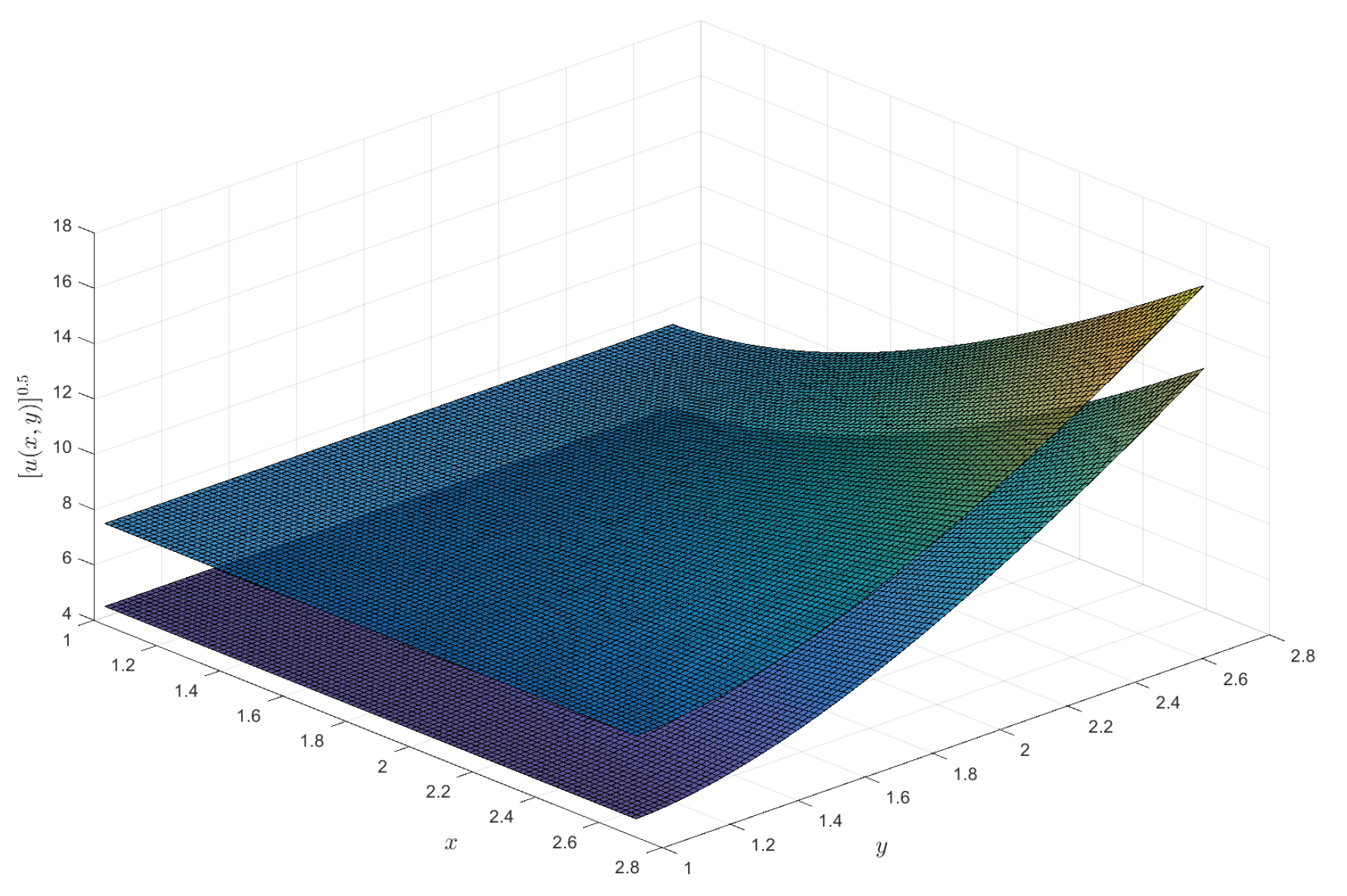
Example 2.
For , the following Caputo-Hadamard fractional differential equation with triangular fuzzy number as the initial value is viewed:
Similarly, we can easily obtain that the system of equations satisfies relevant theorems, so that (28) has solutions . Similar to Example 1, we utilize a numerical method to demonstrate that (28) has a unique solution and leting , then one can easily obtain
Based on Lemma 6 provided earlier, similar to Example 1, we can obtain fuzzy solution:
Next, we will characterize existence and uniqueness of solution to (28) based on r level set of fuzzy solutions:
By utilizing the trapezoidal method for numerical integration defined in Definition 9, We achieve
and for ,
According to (25), one can get for ,
Similar to Example 1, we divide the interval in the same manner, with the set of partition points denoted as and , and the partition distance as . Based on Definition 9 and taking , numerical integration is applied at each mesh point to obtain approximations. Figure 5, Figure 6, Figure 7 and Figure 8 with as and as , respectively. Furthermore, 3D visualizations were generated for different orders on the same level sets (see Figure 5 and Figure 6), as well as for the same order on different level sets (see Figure 7 and Figure 8).
5. Concluding Remarks
The primary purpose of this paper is to focus on existence and uniqueness of solutions for the following FFPDE of Caputo-Hadamard type involving gH-difference:
under some suitable conditions. The classic Caputo FDE had been innovatively extended to Caputo-Hadamard FDE, which held significant meaning due to its integral kernel being in the form of a logarithm rather than the traditional sense of subtraction.
Building upon the work of previous researchers, the main innovations and objectives of this paper are as follows:
(i) In the context of Goursat problems, we extended traditional Caputo FDEs to Caputo-Hadamard FDEs, thereby altering the form of the integral kernel.
(ii) We established the uniqueness and existence of solution to problem (29) using Banach fixed point theorem and Schauder fixed point theorem, rather than relying on metric fixed point theory for verification.
(iii) We presented relevant numerical examples applicable to existence and uniqueness theorem, and further obtained an approximate numerical solution for (29) by discretizing .
In disciplines such as finance, operations research, optics, medicine, biology, engineering, and other practical applications, time delays and pulse effects often arise due to instrument measurements or human interventions. A valuable potential direction for future work is to investigate whether the solution of (29) maintains existence and uniqueness under time delay and during the occurrence of the pulse phenomenon.
Author Contributions
Conceptualization, S.-Y.L. and H.-Y.L.; methodology, S.-Y.L. and H.-Y.L.; software, S.-Y.L. and J.-H.L.; validation, S.-Y.L., H.-Y.L. and J.-H.L.; investigation, S.-Y.L. and H.-Y.L.; writing-original draft preparation, S.-Y.L.; writing-review and editing, S.-Y.L., H.-Y.L. and J.-H.L.; visualization, S.-Y.L. and J.-H.L.; project administration, H.-Y.L.; funding acquisition S.-Y.L., H.-Y.L. and J.-H.L. All authors read and approved the final manuscript.
Funding
This work was partially supported by the Innovation Fund of Postgraduates, Sichuan University of Science & Engineering (Grant number Y2024338), the Scientific Research and Innovation Team Program of Sichuan University of Science and Technology (SUSE652B002) and the Opening Project of Sichuan Province University Key Laboratory of Bridge Non-destruction Detecting and Engineering Computing (Grant number 2024QZJ01).
Conflicts of Interest
The authors declare that they have no conflict of interest.
Abbreviations
The following abbreviations are used in this manuscript:
| H-differential | Hukuhara differential |
| - | generalized Hukuhara |
| FDE | fractional-order differential equation |
| FFDE | fuzzy fractional-order differential equation |
| FFPDE | fuzzy fractional partial differential equation |
References
- Sarwar, M.; Jamal, N.; Abodayeh, K.; et al. Existence and uniqueness result for fuzzy fractional order goursat partial differential equations. Fractal Fract 2024, 8, Paper No. 250, 20 pp. [CrossRef]
- Zadeh, L.A. fuzzy sets. Inf. Control 1965, 8, 338–353. [CrossRef]
- Bers, L.; John, F.; Schechter, M. Partial differential equations. Lectures in Applied Mathematics, volume 3, American Mathematical Society, Rhode Island, 1964.
- Buckley, J.J.; Feuring, T. Introduction to fuzzy partial differential equations. Fuzzy Sets and Systems 1999, 105, 241–248. [CrossRef]
- Cevikel, A.C.; Aksoy, E. Soliton solutions of nonlinear fractional differential equations with their applications in mathematical physics. Rev. Mexicana Fís. 2021, 67, 422–428. [CrossRef]
- SM, S.; Kumar, P.; Govindaraj, V. A novel optimization-based physics-informed neural network scheme for solving fractional differential equations. Eng. Comput. 2024, 40, 855–865.
- Boukhouima, A.; Hattaf, K.; Lotfi, E. M.; et al. Lyapunov functions for fractional-order systems in biology: Methods and applications. Chaos Solitons Fractals 2020, 140, 110224, 9 pp. [CrossRef]
- Du, M. J.; Sun, B. J.; Kai, G. Adaptive multi-step piecewise interpolation reproducing kernel method for solving the nonlinear time-fractional partial differential equation arising from financial economics. Chin. Phys. B. 2023, 32 (3), 030202.
- Tarasov, V.E. Nonlocal statistical mechanics: General fractional liouville equations and their solutions. Phys. A. 2023, 609, Paper No. 128366, 40 pp. [CrossRef]
- Murio, D.A. Stable numerical evaluation of grünwald–letnikov fractional derivatives applied to a fractional IHCP. Inverse Probl. Sci. Eng. 2009, 17, 229–243. [CrossRef]
- Luchko, Y.; Trujillo, J. Caputo-type modification of the erdélyi-kober fractional derivative. Fract. Calc. Appl. Anal. 2007, 10, 249–267.
- Fan, E.Y.; Li, C.P.; Li, Z.Q. Numerical approaches to Caputo-Hadamard fractional derivatives with applications to long-term integration of fractional differential systems. Commun. Nonlinear Sci. Numer. Simul. 2022, 106, Paper No. 106096, 34 pp. [CrossRef]
- Allahviranloo, T. Fuzzy fractional differential operators and equations-fuzzy fractional differential equations. Studies in Fuzziness and Soft Computing, volume 397, Springer, Cham, 2021.
- Salahshour, S.; Allahviranloo, T.; Abbasbandy, S. Solving fuzzy fractional differential equations by fuzzy Laplace transforms. Commun. Nonlinear Sci. Numer. Simul. 2012, 17, 1372–1381.
- Arqub, O.A.; Al-Smadi, M. Fuzzy conformable fractional differential equations: Novel extended approach and new numerical solutions. Soft comput. 2020, 24, 12501–12522. [CrossRef]
- Ahmadian, A.; Suleiman, M.; Salahshour, S.; et al. A jacobi operational matrix for solving a fuzzy linear fractional differential equation. Adv. Difference Equ. 2013, 2013, 104, 29 pp.
- Akram, M.; Ihsan, T. Solving pythagorean fuzzy partial fractional diffusion model using the Laplace and Fourier transforms. Granul. Compu. 2023, 8, 689–707.
- Alderremy, A.; Gómez-Aguilar, J.F.; Aly, S. A fuzzy fractional model of coronavirus (covid-19) and its study with legendre spectral method. Results. Phys. 2021, 21, Paper No. 103773, 10 pp.
- Abuasbeh, K.; Shafqat, R. Fractional Brownian motion for a system of fuzzy fractional stochastic differential equation. J. Math. 2022, 2022, Art. ID 3559035, 14 pp. [CrossRef]
- Askari, S.; Allahviranloo, T.; Abbasbandy, S. Solving fuzzy fractional differential equations by adomian decomposition method used in optimal control theory. Int, Trans. Eng. Manag. Appl. Sci. Technol. 2019, 10, Paper ID: 10A12P, 10 pp.
- Keshavarz, M.; Qahremani, E.; Allahviranloo, T. Solving a fuzzy fractional diffusion model for cancer tumor by using fuzzy transforms. Fuzzy Sets and Systems. 2022, 443, 198–220.
- Aliev, R.A.; Pedrycz, W.; Huseynov, O.H. Hukuhara difference of z-numbers. Inform. Sci. 2018, 466, 13–24.
- Amma, B.B.; Melliani, S.; Chadli, L.S. On the existence and uniqueness results for intuitionistic fuzzy partial differential equations. Int. J. Dyn. Syst. Differ. Equ. 2023, 13, 22–43. [CrossRef]
- Tao, J.; Zhang, Z.H. Properties of interval-valued function space under the gH-difference and their application to semi-linear interval differential equations. Adv. Difference Equ. 2016, 2016, Paper No. 45, 28 pp.
- Ghaffari, M.; Allahviranloo, T.; Abbasbandy, S.; et al. Generalized Hukuhara conformable fractional derivative and its application to fuzzy fractional partial differential equations. Soft comput. 2022, 26, 2135–2146. [CrossRef]
- Zhang, F.; Xu, H.Y.; Lan, H.Y. Initial value problems of fuzzy fractional coupled partial differential equations with Caputo gH-type derivatives. Fractal Fract. 2022, 6, Paper No. 132, 24 pp.
- Gohar, M.; Li, C.P.; Yin, C.T. On Caputo–Hadamard fractional differential equations. Int. Comput. Cent., Bull. 2020, 97, 1459–1483.
- Dhali, M.N.; Bulbul, M.F.; Sadiya, U. Comparison on trapezoidal and Simpson’s rule for unequal data space. Int. J. Math. Sci. Comput. 2019, 5, 33–43.
- Diamond, P.; Kloeden, P. Metric spaces of fuzzy sets. Fuzzy Sets and Systems 1990, 35, 241–249. [CrossRef]
- Long, H.V.; Son, N.T.K.; Tam, H.T.T. The solvability of fuzzy fractional partial differential equations under Caputo gH-differentiability. Fuzzy Sets and Systems 2017, 309, 35–63. [CrossRef]
- Stefanini, L. A generalization of Hukuhara difference and division for interval and fuzzy arithmetic. Fuzzy Sets and Systems 2010, 161, 1564–1584.
- Allahviranloo, T.; Gouyandeh, Z.; Armand, A.; et al. On fuzzy solutions for heat equation based on generalized Hukuhara differentiability. Fuzzy Sets and Systems 2015, 265, 1–23.
- Salahshour, S.; Allahviranloo, T.; Abbasbandy, S.; et al. Existence and uniqueness results for fractional differential equations with uncertainty. Adv. Difference Equ. 2012, 2012, 112, 12 pp. [CrossRef]
- Agarwal, R.P.; Meehan, M.; O’regan, D. Fixed Point Theory and Applications. Cambridge university press, Cambridge, 2001.
- An, T.V.; Vu, H.; Van Hoa, N. The existence of solutions for an initial value problem of Caputo-Hadamard -type fuzzy fractional differential equations of order α∈(1,2). J. Intell. Fuzzy Systems. 2019, 36, 5821–5834. [CrossRef]
- Jarad, F.; Abdeljawad, T.; Baleanu, D. Caputo-type modification of the Hadamard fractional derivatives. Adv. Difference Equ. 2012, 2012, 142, 8 pp.
Figure 1.
Fuzzy solution for .
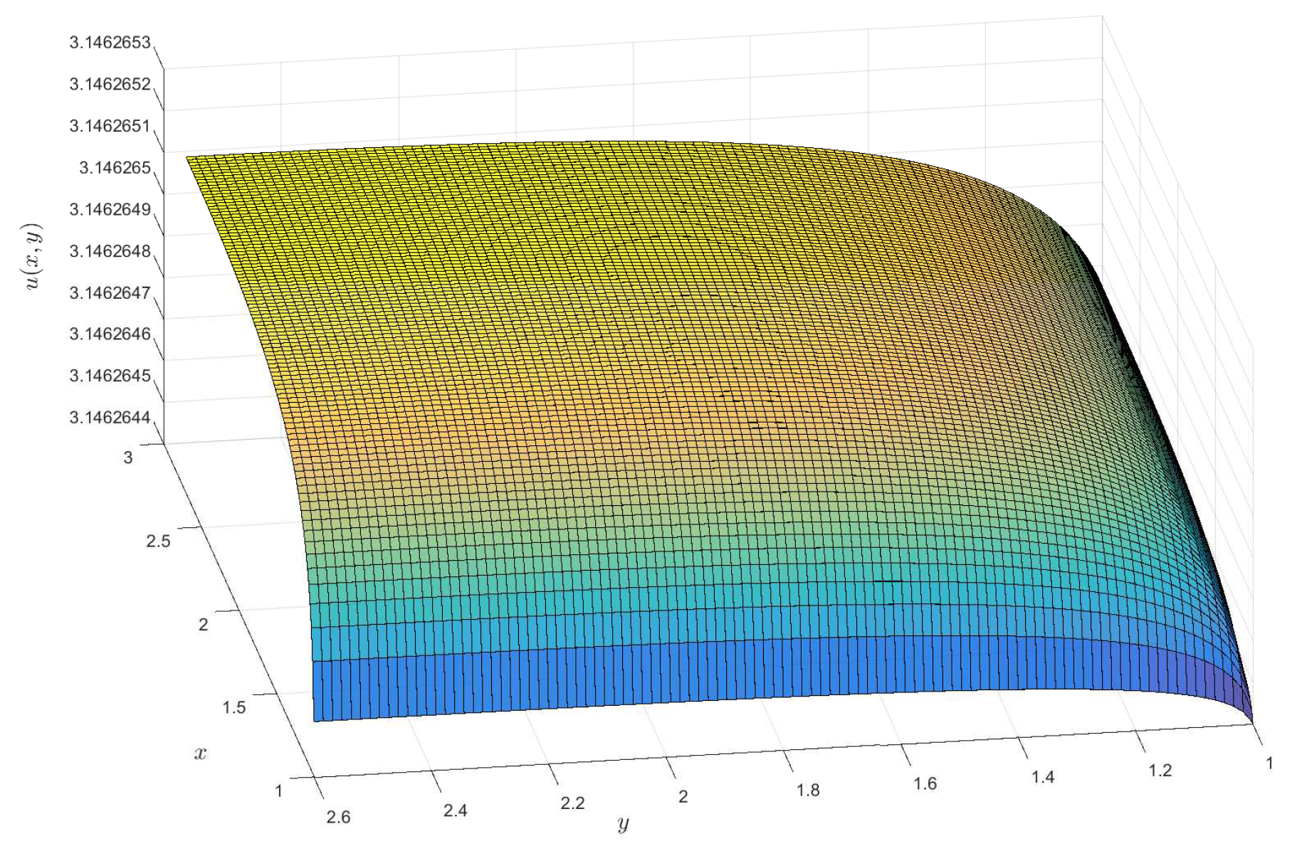
Figure 2.
Fuzzy solution with .
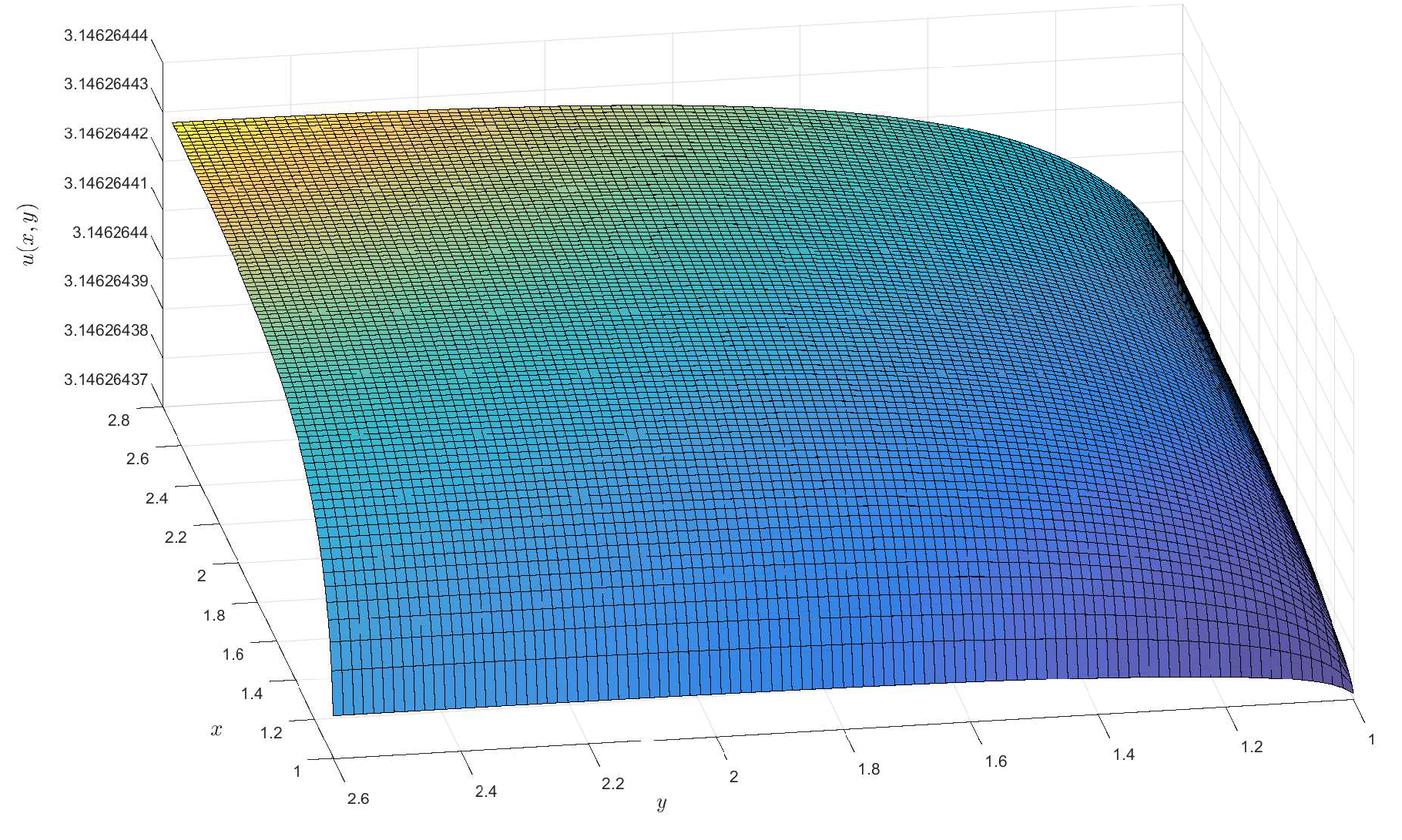
Figure 3.
Fuzzy solution with .
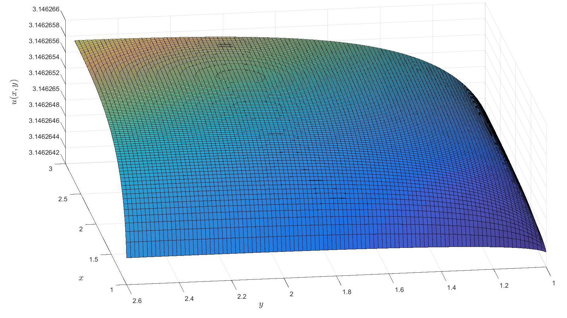
Figure 4.
Fuzzy solution for .
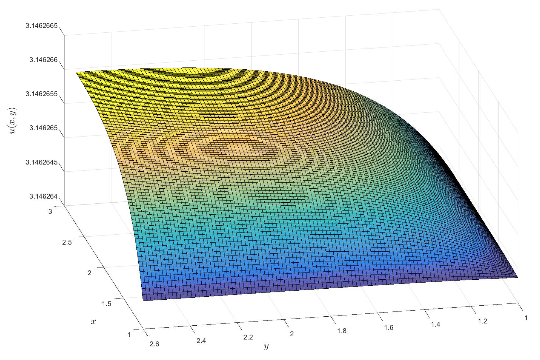
Figure 5.
The level set of fuzzy solutions for (28) under and .
Figure 5.
The level set of fuzzy solutions for (28) under and .
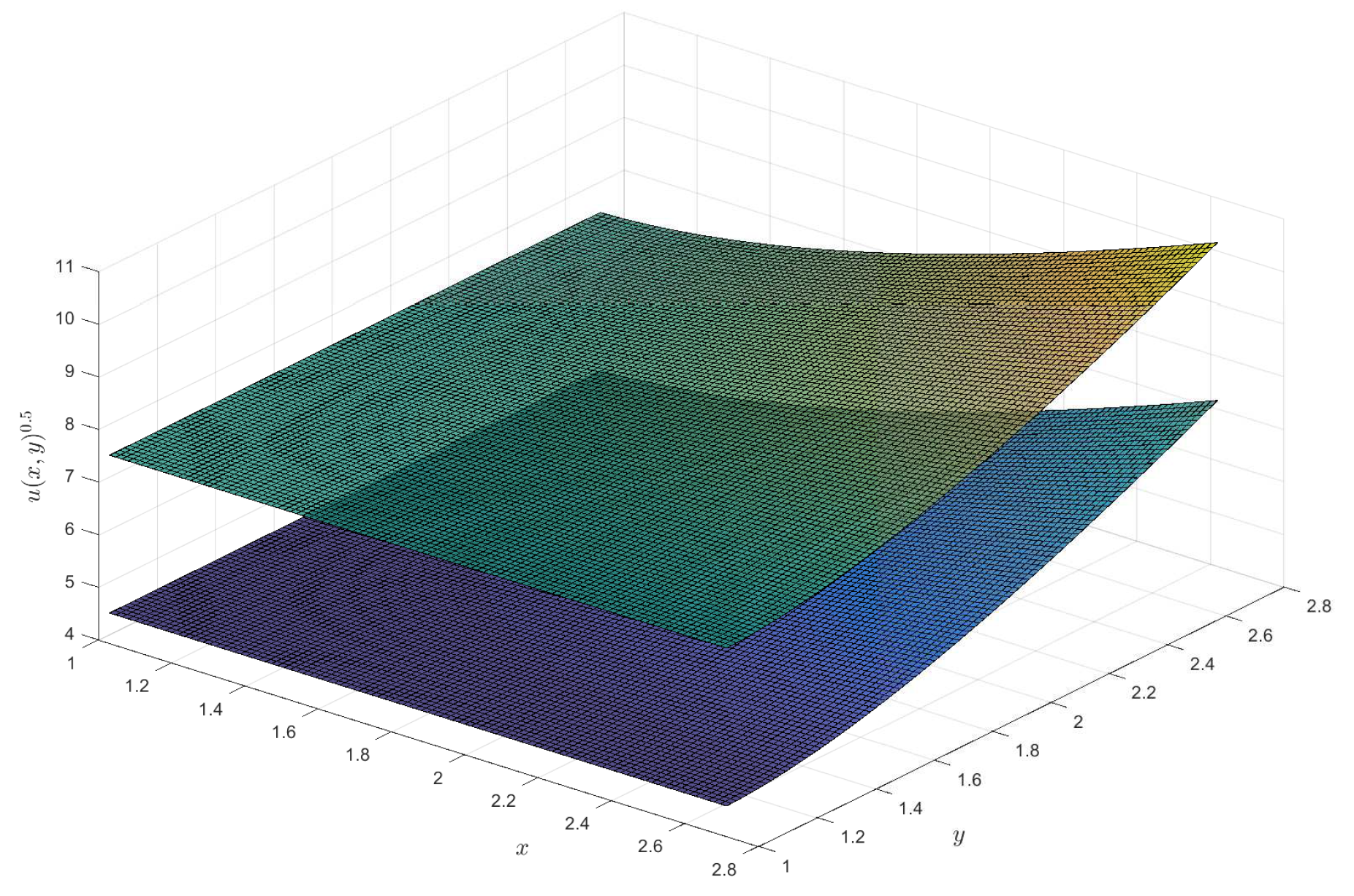
Figure 6.
The level set of fuzzy solutions for (28) under and .
Figure 6.
The level set of fuzzy solutions for (28) under and .
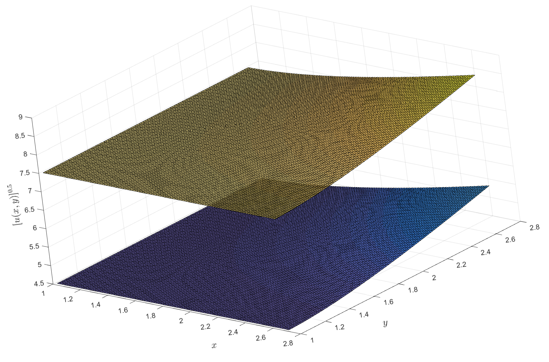
Figure 7.
The level set of fuzzy solutions for (28) as and .
Figure 7.
The level set of fuzzy solutions for (28) as and .
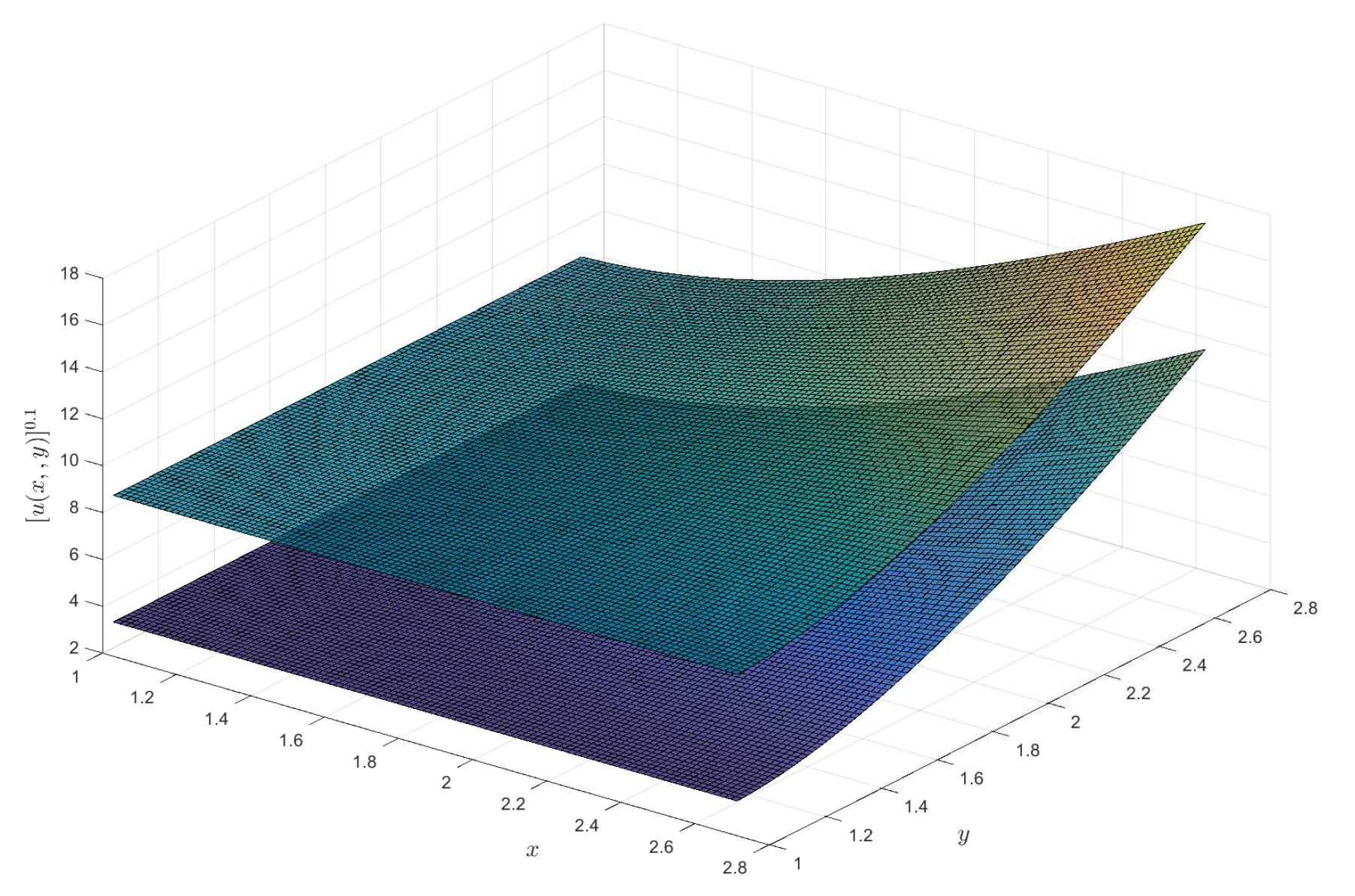
Figure 8.
The level set of fuzzy solutions for (28) as and .
Figure 8.
The level set of fuzzy solutions for (28) as and .
Disclaimer/Publisher’s Note: The statements, opinions and data contained in all publications are solely those of the individual author(s) and contributor(s) and not of MDPI and/or the editor(s). MDPI and/or the editor(s) disclaim responsibility for any injury to people or property resulting from any ideas, methods, instructions or products referred to in the content. |
© 2025 by the authors. Licensee MDPI, Basel, Switzerland. This article is an open access article distributed under the terms and conditions of the Creative Commons Attribution (CC BY) license (http://creativecommons.org/licenses/by/4.0/).
Copyright: This open access article is published under a Creative Commons CC BY 4.0 license, which permit the free download, distribution, and reuse, provided that the author and preprint are cited in any reuse.


