Submitted:
22 May 2025
Posted:
23 May 2025
You are already at the latest version
Abstract
This study investigates whether, when using multispectral imagery, it is preferable to retrain a random forest model once a year or to train it for a single year and then use that model to predict all subsequent years. We utilized Sentinel-2 images as the primary input features along with environmental data for the study. The targets representing both natural and semi-natural habitats for classification were used in an area of central Italy. By excluding all burned areas since 2001, we assessed the area’s stability over the past nine years. The approach involved conducting a twin experiment to compare the results of model training and predictions under two distinct scenarios. In the initial experiment, named SINGLE, the model was trained using data from one year (2023) and subsequently applied to generate land cover maps spanning from 2016 to 2024. In the second experiment, known as MULTI, the model undergoes annual retraining before forecasting the land cover for each respective year. The findings reveal that in the MULTI experiment, the accuracies are not only superior to those in the SINGLE experiment but also exhibit consistent stability, highlighting the effectiveness of annual model retraining.
Keywords:
random forest
; training
; multispectral
1. Introduction
Earth observation tools and techniques offer valuable spatial information, allowing researchers to assess land cover [1,2,3] across different regions and time periods. This capability also allows for an evaluation of the current distribution of land cover, especially focusing on vegetation [4]. The detection of ecosystems and the estimation of their distribution using aerial and satellite imagery [5] have sparked increased interest in enhancing the understanding of habitat distribution and dynamics [6,7,8]. One of the key goals of national and regional government agencies is to manage and monitor the condition of natural resources within their areas of responsibility [9]. Satellite-based habitat monitoring aids in identifying habitats and monitoring changes resulting from environmental shifts [10], climate change [11], as well as human and natural disruptions like wildfires [12], logging [13], and pest outbreaks [14]. These changes can occur across varying spatial and temporal scales [15,16,17,18,19] highlighting the essential need for ecosystem monitoring on a broad spatial scale. Therefore, it should be feasible to assess and document the impacts on various ecosystems at regional and national scales resulting from land degradation and disturbances [8]. It is therefore crucial to have remote sensing data and distribution model methods that can accurately identify and distinguish between various habitats, as both climatic and human-induced transformations can significantly impact the condition of these ecosystems. Essential criteria for long-term ecosystem monitoring include being an easily applicable and repeatable technique utilizing readily available and accessible data [2], and having the capability to map trends at a large scale while assessing the status of different habitats over extended periods of time [20]. A significant body of literature [21,22,23] supports the idea that predicting land cover maps with models involves addressing uncertainties in land cover classification. Stehman and Foody (2019) [23] emphasized the significance of evaluating map quality, highlighting the evolution of techniques such as sampling and error matrix. Accuracy assessment currently relies on a good practice methodology consisting of three key components: sampling design, response design, and analysis [24]. It is essential to meticulously analyze land cover maps to maximize their utility. To achieve this, it is crucial to comprehend how models operate based on the input features provided, enabling their calibration for accurate predictions of land cover maps. Hence, in addition to model accuracy, the calibration and prediction strategy can alter model outcomes, especially when employing optical sensors that are responsive to vegetation phenology.
Generally, two primary strategies are utilized to classify land cover changes by satellite time-series data [25]. The first method involves producing separate land cover maps for each time point (e.g., each year), which is useful for detecting cover changes over a specific time period [26]. This enables the calibration of the model with actual monthly time series, which are typically computed annually to reflect seasonal changes. This approach relies on the portability of the models and the availability of surface reflectance values, which are essential for extending land cover [25]. The second method entails establishing a base map from a specific year’s reference date and subsequently projecting it annually by integrating change information derived from the spectral time series. According to this method, it enables the detection of various types of changes, such as subtle or significant shifts, as well as the absence of change [27]. In this context, Sittaro et al. (2022) [8] utilized an ensemble approach with three models trained on different years (2013, 2014, and 2016) to classify vegetation habitats in Germany for the years 2010 and 2019 to evaluate the habitat changes. To address these challenges, we investigate the question: what is the most effective modeling approach for spatial habitat detection, multi-training or multi-projection? In the multi-training approach, a distinct model is trained for each time point using data specific to that period, enabling the capture of temporal variations within each model. In contrast, the multi-projection approach involves training a single model on data from one time point and then applying it to subsequent time points to detect changes. This research thus explores the effectiveness of annually retraining the model versus training a single model for a specific year and using it for classification across multiple years. Random Forest models were used along with Sentinel-2 spectral data, environmental variables, and ground truth observations in a twin experiment to solve this problem. In the first experiment, a multi-training strategy was employed, where separate models were trained for each year. Otherwise, the second experiment followed a multi-projection approach, wherein a single model was calibrated using data from a reference year and subsequently applied to predict land cover across a nine-year period. The paper is structured as follows: Section 2 describes the methodology; Section 3 presents the results and accuracy assessments; Section 4 discusses the findings significance; and Section 5 provides the conclusions.
2. Materials and Methods
In the first experiment, called MULTI, the random forest model was trained with the annual Sentinel-2 time series data from each specific year to predict land cover in our study area. Therefore, we have had multiple models used over the years. In the second experiment, called SINGLE, the model was trained using the annual time series of a specific reference year (2023), and this model was then applied to predict land cover across the years using the corresponding Sentinel-2 observations. In this context, we are assuming that the characteristics of our study area remained consistent throughout the time period under consideration.
2.1. Study Area and Target Definition
This study aims to classify vegetation habitats in the Monti Pisani massif (Figure 1), in central Italy, a minor segment of the Northern Apennines that is geographically isolated from the rest of the mountain range, making it a distinct and separate entity. The Monti Pisani, situated between the provinces of Pisa and Lucca in Tuscany, is characterized by moderately elevated terrain. Its highest point rises to an altitude of 917 m above sea level, situated adjacent to the plain of Pisa to the northeast (Figure A1).
The Monti Pisani area has a long history of agrosilvopastoral activities, which have significantly shaped the landscape over time. Practices such as agricultural terracing, selective logging, and seasonal grazing have affected vegetation cover, soil stability, and forest structure. The vegetation in Monti Pisani consists mainly of maritime pine and holm oak forests on the western slopes, with coppice chestnut woodlands prevailing in the northern and eastern regions. The Monti Pisani massif is also characterized by patches of garrigue and evergreen shrubs in different stages of growth, which are often remnants of past wildfires [28]. Extensive olive groves are found along the transition zone between rural and natural areas, representing a traditional and historical form of cultivation typical of the Mediterranean region. They are embedded in the natural landscape, and sometimes, because they are also often neglected [29] they can be added to the natural habitats.
Historically, wildfires have been the primary disturbances affecting the Monti Pisani area, especially impacting the eastern and southern slopes of the massif. In 2018–2019, extensive wildfires caused significant changes in land cover and disrupted the ecological balance of the impacted ecosystems. For research reliability, areas impacted by wildfires post-2001 (as documented by the Tuscany region) were intentionally left out of the study area. This method ensures that bias from changes in ecological conditions in those regions is minimized. Additionally, while nearby human settlements may introduce some level of disturbance, we consider these effects to be minimal and unlikely to influence the broader outcomes of the study.
We detected eight main vegetation types from the study area based on their distribution: grassland (G), rocky habitat or screes (SC), needle-leaved shrub (N), evergreen shrubland (S), broadleaved deciduous forests (T1), broadleaved evergreen forests (T2), coniferous forests (T3), and olive groves (OG).
Table 1 shows the number of targets used for classification for each target class. The majority of the targets were surveyed and captured between November 2023 and January 2024. We collected 329 target points around and in the area of Monti Pisani (Figure 1). The number of target points corresponds to the anticipated quantity based on the distribution of vegetation classes in the specified region.
In order to avoid spurious accuracy due to spatial autocorrelation that is often present in land cover, the target points are isolated points; there may be points with the same class that are close, but they are not contiguous. Using isolated target points for model validation ensures a robust assessment of the model accuracy in predicting land cover within the specified regions of interest. This rigorous approach not only eliminates potential biases but also ensures a more reliable assessment of the model’s performance.
2.2. Features
A spatially explicit dataset of predictor variables was developed to generate classified habitat maps using the selected classification method. The predictors are grouped into two main categories:
- Environmental data: variables pertaining to geographic, topographic, climatic, and property characteristics.
- Spectral data: values derived from Earth observation satellite sensors.
All variables were obtained or calculated from datasets released under open-access policies and resampled to a common spatial resolution of 20 meters. The reference spatial grid is based on the EPSG:32632 coordinate system and has a 20-meter spatial resolution. It matches the Sentinel-2 tile T32TPP, which covers the Monti Pisani. Environmental variables were selected based on their relevance to plant dispersal processes [30,31].
The linear distances in kilometers from both the seashore and the river network were calculated for each grid cell among the geographic variables [32]. A digital elevation model of Italy at 20 m [33] with a spatial resolution of 20 m was used to calculate elevation, slope, and aspect by analyzing a 3 × 3 pixel neighborhood. From the aspect values, the northernness and easternness components were computed using sine and cosine transformations to generate continuous variables. The total amount of rain [34] and the average temperature [35] at a resolution of 1 km were interpolated from the coordinates of the cell’s center to the resolution of the reference grid using a regularized spline with tension. The average temperature was adjusted for altitude effects to render it independent of elevation. The daily average solar irradiance was calculated at a spatial resolution of 20 m using equations for solar energy-related characteristics, taking local topography into account. The monthly averages of daily solar irradiance and the monthly average climatological cloud cover percentage [36] were also derived. The daytime cloud cover data, obtained from the ESA Climate Change Initiative (CCI) dataset for the year 2014, were resampled using a regularized spline to match the 20-meter resolution [37], allowing for better estimation of sky diffuse radiation. The result was a monthly weighted solar irradiance dataset used to compute daily averages. Soil properties, specifically pH and depth to bedrock, were extracted from the SoilGrids dataset [38], originally at 250 meter resolution, and interpolated to the reference grid using a Bartlett filter with a 750-meter radius. The Copernicus High Resolution Layer for Tree Cover Density was also incorporated and resampled to 20 meters. Spectral data included surface reflectance bands and derived spectral indices from Sentinel-2’s Multi-Spectral Instrument (MSI), which features high spatial resolution (10 m, 20 m, and 60 m), a five-day revisit time, a 290 km swath width, and a spectral range spanning from visible to shortwave infrared [39,40]. All Sentinel-2 images acquired from 2016 to 2024 with cloud cover below 90% were collected. Surface reflectance bands were resampled to a uniform resolution of 20 meters, creating a consistent dataset with the following bands: B2 (blue), B3 (green), B4 (red), B5–B7 (red edge 1–3), B8 (NIR1), B8a (NIR2), B11 (SWIR1), and B12 (SWIR2). Monthly averages were computed to generate annual time series. Missing data were imputed using the imputeTS R package [41]. Additional quality indicators were calculated to assess the effects of slope and sun zenith angle on pixel values, leading to the creation of topographic and low sun masks. The final classification relied on the full set of Sentinel-2 MSI bands (January–December) and four spectral indices: EVI, NDYI, RI, and CRI1 as described in Table 2 and further detailed in Agrillo et al. (2021) [42].
2.3. Model Strategy and Validation
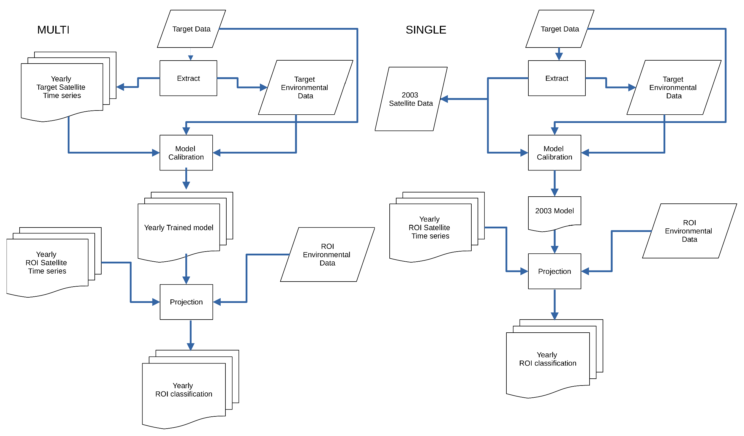
Our goal is to evaluate how well different models reproduce land cover, assuming no significant changes occurred over the nine-year period from 2016 to 2024. Two approaches were applied to classify land cover in the Monti Pisani region. In the first approach, a new classification model was trained each year using satellite imagery time series of a specific year, along with the environmental predictor variables. This model was used to classify land cover without reusing the previous model. This resulted in a model being retrained annually. Each yearly model was then used to classify every pixel in the study area, producing an annual land cover map based on Sentinel-2 data. In the second approach, a single model was trained using data from a reference year to maintain consistency over time. The year 2023 was selected as the base year, since the ground truth (target) points were collected between the end of 2023 and the beginning of 2024. This model was then used to classify land cover for all other years using the corresponding satellite imagery, without further retraining. Figure A2 shows the workflow of these two strategies. Both classification strategies used the ranger R package [47], an efficient implementation of the Random Forest algorithm [48] particularly suited for high-dimensional data. The algorithm supports classification, regression, and survival analysis and includes features such as randomized trees [49] and quantile regression forests [50].
All available predictor variables were used as inputs, since Random Forest is robust to multicollinearity among predictors [51]. The only problem that correlated data have using RF concerns the variable importance, which is not relevant for this study.
Although, during the calibration stage, 80% of targets were used for training and 20% for testing, during the prediction stage, all the points in the area of interest were used to figure out how well the models actually predicted the land cover in that area, since a comparison of the entire map with the reference data is both arduous and virtually impossible [52,53]. The error matrix characterizes the comparison results, allowing for the calculation of accuracy measures such as overall accuracy, Kappa, user accuracy, and producer accuracy [54]. However, due to the large number of years and land cover classes (which would result in 64 user and producer accuracy scores), the analysis focused solely on overall accuracy. To assess the reliability of accuracy and area estimates, the standard error was calculated following the methodology of Olofsson et al. (2013) [55]. To examine the temporal stability of classification results, we computed the coefficient of variation (CV) [56] for each land cover class. This metric enables a straightforward comparison of how variability differs across different classes over time. The CV is defined as
where and are, respectively, the standard deviation and mean computed over the years of the number of pixels of class C. CV provides a normalized measure of prediction consistency across time and allows us to assess the consistency of predicted values across different time periods, providing a normalized variability measure that provides insight into the reliability of the model predictions.
3. Results
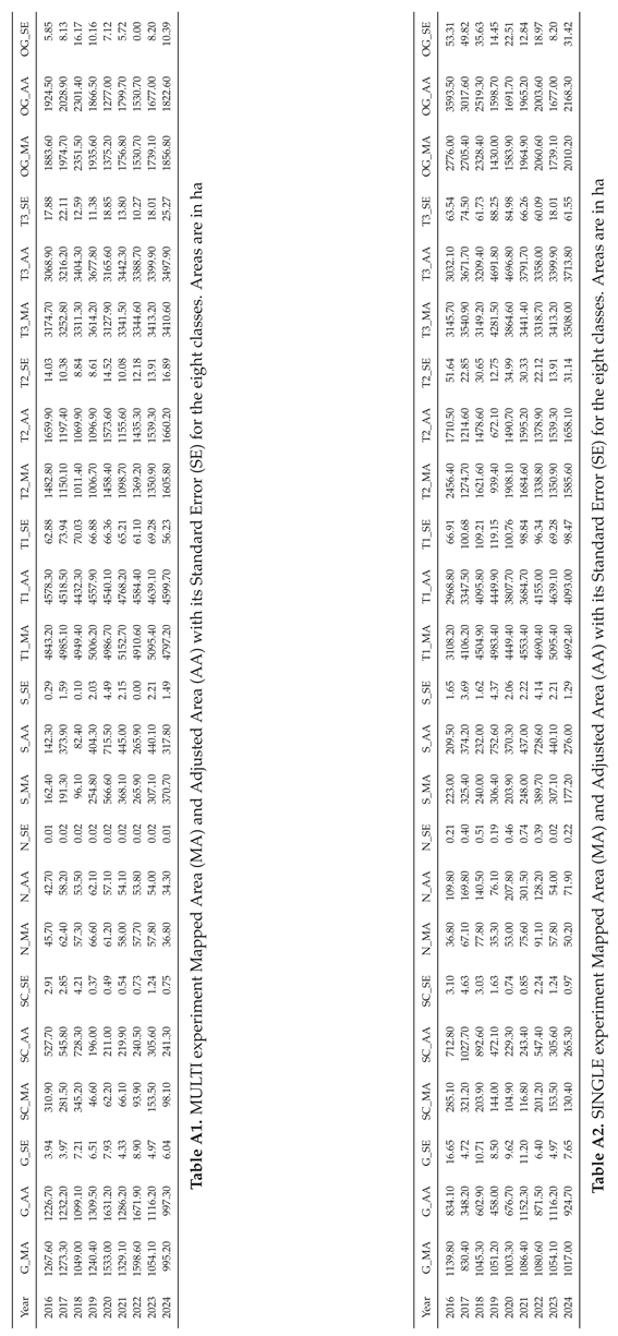
The evaluation approach is based on the assumption that the region of interest was minimally disturbed. Areas affected by wildfires post-2000 were intentionally excluded from the Monti Piani region as they are not part of the defined region of interest. Therefore the models using Sentinel-2 predictors are expected to consistently predict the same areas from 2016 to 2024. Tables A1 and A2 present the total mapped areas of each class alongside estimates obtained using the algorithm in Olofsson (2013) [55]. These estimates can be viewed as “error-adjusted” areas because they include the area of map omission error of each category and leave out the area of map commission error. The estimated standard error of the estimated area is also added in Tables A1 and A2 [57]. These tables show that a mapped area is considered accurate when the difference from the adjusted area is minimal.
To assess the variability of computed areas, we calculated the mean, standard deviation, and coefficient of variability, as presented in Table 3. In this context, the results are controversial, with certain classes like grassland, scree, and shrubland showing a lower CV in the SINGLE experiment compared to the MULTI experiment. For example, the grassland area exhibits higher stability in the SINGLE experiment, with a ratio of 0.08, in contrast to the 0.17 value observed in the MULTI experiment. In contrast, the remaining classes, primarily linked to trees, show a higher CV in the SINGLE experiment than in the MULTI experiment. For example, the CV of T1 is only 0.02 in MULTI compared with the value of 0.28 in the SINGLE experiment. We are confident that the low values of CV for the forest classes in the MULTI experiment show the stability of the prediction. The variability observed in the other classes not related to woodland may be attributed to annual fluctuations in vegetation growth. For instance, sparsely vegetated areas may be covered by plants in certain years, leading to their classification as grassland. In other years, when vegetation is minimal, these same areas may be classified as unvegetated areas (e.g., scree).
Thus, another metric to show how the two approaches give different results is the accuracy (Table 4). This accuracy was computed using the predicted classification and all the targets falling in the region of interest, employing a comprehensive evaluation approach. This accuracy differs from the one obtained during the calibration phase, which utilizes a limited dataset to assess the model’s performance, contrasting with the comprehensive evaluation conducted here.
This further supports the notion that the region has remained largely undisturbed, excluding the areas with significant wildfires.By excluding areas affected by fires post-2000, a more accurate and reliable prediction model was developed, enhancing the integrity of the data and analysis in this study.
The accuracies for the MULTI experiment consistently range from 95% to 97%. This consistency in accuracy values over the time-span from 2016 to 2024 indicates the reliability of the prediction model developed for the Monti Pisani region. These findings suggest that the region has indeed remained largely undisturbed. The SINGLE experiment, where the model was trained for one year, 2023, and applied to all years to make predictions for the years from 2016 to 2024, shows that the accuracy changes drastically from year to year. It goes from 96% of the year 2023, which is the year of the predictors to train the model, with a decrease in accuracy that is proportional to the distance from the year 2023, up to 63% of 2016.
Figure 2 displays the modal values of the classification for both the MULTI experiment 2a and the SINGLE experiment 2b, while Figure 3 illustrates the spatial distribution where the two modal values differ. While the distribution of the modal classes is generally similar, variations can be observed in specific regions. Specifically, in the northern region characterized by a strong anthropic presence, the spatial variability of the natural and semi-natural habitats, such as the olive groves, is notably high, leading to more distinct differences in the models.

Table 4.
Overall accuracy and its standard error for the MULTI and SINGLE experiments computed on the predicted classes.
Table 4.
Overall accuracy and its standard error for the MULTI and SINGLE experiments computed on the predicted classes.
| year | MULTI | SINGLE | ||
| OA | SEoa | OA | SEoa | |
| 2016 | 0.956 | 0.014 | 0.660 | 0.029 |
| 2017 | 0.941 | 0.016 | 0.675 | 0.029 |
| 2018 | 0.944 | 0.016 | 0.702 | 0.029 |
| 2019 | 0.956 | 0.015 | 0.742 | 0.027 |
| 2020 | 0.948 | 0.015 | 0.727 | 0.028 |
| 2021 | 0.960 | 0.014 | 0.792 | 0.026 |
| 2022 | 0.966 | 0.013 | 0.812 | 0.025 |
| 2023 | 0.953 | 0.015 | 0.953 | 0.015 |
| 2024 | 0.949 | 0.015 | 0.795 | 0.027 |
Changes during yearly classification can be seen by evaluating the number of changes of single pixels, normalized by the number of years. The parameter for pixel stability (PS) is calculated using the following equation:
where T-1 represents the maximum number of changes. This gives a value between 0 and 1, where the value 1 indicates no change and 0 indicates maximum change. Figure 4 shows the pixel stability for the MULTI and SINGLE experiments. A clear distinction is observed, with the MULTI experiment showing a significantly larger unchanged area compared to the SINGLE experiment. The susceptibility to change in an area in the northern part of the Monti Pisani massif is likely influenced by its proximity to a region with significant human activity, which can lead to more pronounced changes due to anthropogenic influences, as depicted in Figure 2.
4. Discussion
Choosing the right training strategy is crucial for accurate land cover classifications in environments with varying seasons [58,59,60,61]. We compared two strategies in training a model to classify natural land-cover:
- A multiyear approach (MULTI) involves using the same set of satellite images from each year to train the model and categorize the land cover.
- A single-year approach (SINGLE), where the model is trained by a single-year satellite imagery time series (in our case 2023), and it is used to classify the land cover backward and forward through its projection.
The study provides specific evidence that the MULTI approach achieves superior classification performance by training the model on the exact dataset used for classifying natural land cover.
The MULTI approach consistently achieved classification accuracies between 95% and 97%, confirming its robustness across multiple years. Conversely, the SINGLE experiment, which trains the model on data from a single year and uses it across multiple years, experienced a significant decrease in accuracy over time, reaching as low as 63% in years distant from the training year. In the MULTI approach, the model considers changes in yearly remote sensing data and environmental conditions more effectively.
The SINGLE model, while potentially applicable in scenario-based studies involving future predictors (e.g., climate projections), shows significant performance loss when applied to past or future years without temporal adaptation.
This difference is especially important in the Mediterranean, where changes in temperature and rainfall from year to year [62] have a substantial impact on the growth cycles and habitat suitability of different plant species.
Based on our twin experiments, it is evident that training the model on an annual basis allows it to effectively capture fluctuations in satellite observations driven by phenological trends in vegetated areas. In contrast, regions with stable phenological patterns, such as equatorial zones, tend to exhibit more consistent spectral distributions, including reflectance values across specific bands, over multiple years. In such environments, a single-year-trained model may also perform well. Our results are limited to the Mediterranean climate region, where landscapes exhibit annual variation driven by the thermo-pluviometric regime [63]. Accurately capturing these seasonal dynamics is essential for maintaining high accuracy when performing land-cover classification [64,65]. Further support comes from the analysis of vegetation reflectance variability over time. Figure 5 illustrates the average value of the Band 8, corresponding to the Near Infrared (NIR) band, averaged on April for eight land cover classes, showing noticeable year-to-year variation even within the same class. This variability is not arbitrary but stems from actual phenological shifts influenced by dynamic changes in climatic conditions, underscoring the sensitivity of vegetation to environmental fluctuations [66,67]. Because random forest classifiers use feature thresholds, these changes between years can cause the decision boundaries to shift significantly, potentially impacting the accuracy of the model.
5. Conclusions
Synchronizing training and prediction data in time is crucial for effective land cover classification using multispectral satellite imagery, like that from Sentinel-2’s MSI sensor. Multispectral reflectance values can vary over time due to both actual land cover changes (e.g., disturbances) and subtle shifts in natural vegetation growth dynamics influenced by interannual climate fluctuations. The results unequivocally demonstrate that training classification models with the same yearly time series used for predicting land cover for that year significantly enhances performance. These findings emphasize that misalignment between training and prediction features significantly diminishes the model’s ability to perform well across years, especially in regions with high environmental variability, like the Mediterranean biogeographical region. Furthermore, aligning training and prediction data enhances not only accuracy but also the reliability and interpretability of land cover classifications over time. Regularly checking and adapting to changes over time helps models stay updated on shifts in land cover, providing a clearer and more relevant view of how landscapes change. In the end, this study shows an important idea in the field of remote sensing-based land cover classification: the stability and representativeness of the training dataset are crucial for making sure that predictions are consistent and correct. Ensuring the model learns from a diverse and accurate dataset is essential for generating robust and reliable classification outcomes. In regions experiencing substantial environmental changes, it is crucial to adopt a multi-year modeling approach that can adapt to dynamic shifts for effective long-term monitoring and change detection.
Author Contributions
Conceptualization, N.T., A.P., E.A., A.M.; methodology, N.T. and E.A.; software, N.T.; validation, N.T., E.A., A.P. and A.M.; investigation, N.T.,E.A., A.P, A.M..; data curation, N.T., E.A., A.P. and A.M.; writing—original draft preparation, N.T.; writing—review and editing, N.T., E.A., A.P. and A.M.; All authors have read and agreed to the published version of the manuscript.
Funding
This research received no external funding.
Data Availability Statement
Sentinel-2 multispectral data can be obtained by the Copernicus Data Space Environment https://dataspace.copernicus.eu, results of the classification are available upon request.
Acknowledgments
We acknowledge Mara Baudena, Paolo Fiorucci and other participants of the Spoke 4 “Ecosystem functions, services and solutions” of the National Biodiversity Future Center for some useful discussions.
Conflicts of Interest
The authors declare no conflicts of interest.
Appendix A
In this appendix, there are two complementary figures and two complementary tables.
Figure A1.
Region of Interest: the Monti Pisani massif, without the burned areas from 2001 onward. It is located in the western part of the Tuscany region. Main cities and topography are shown.
Figure A1.
Region of Interest: the Monti Pisani massif, without the burned areas from 2001 onward. It is located in the western part of the Tuscany region. Main cities and topography are shown.
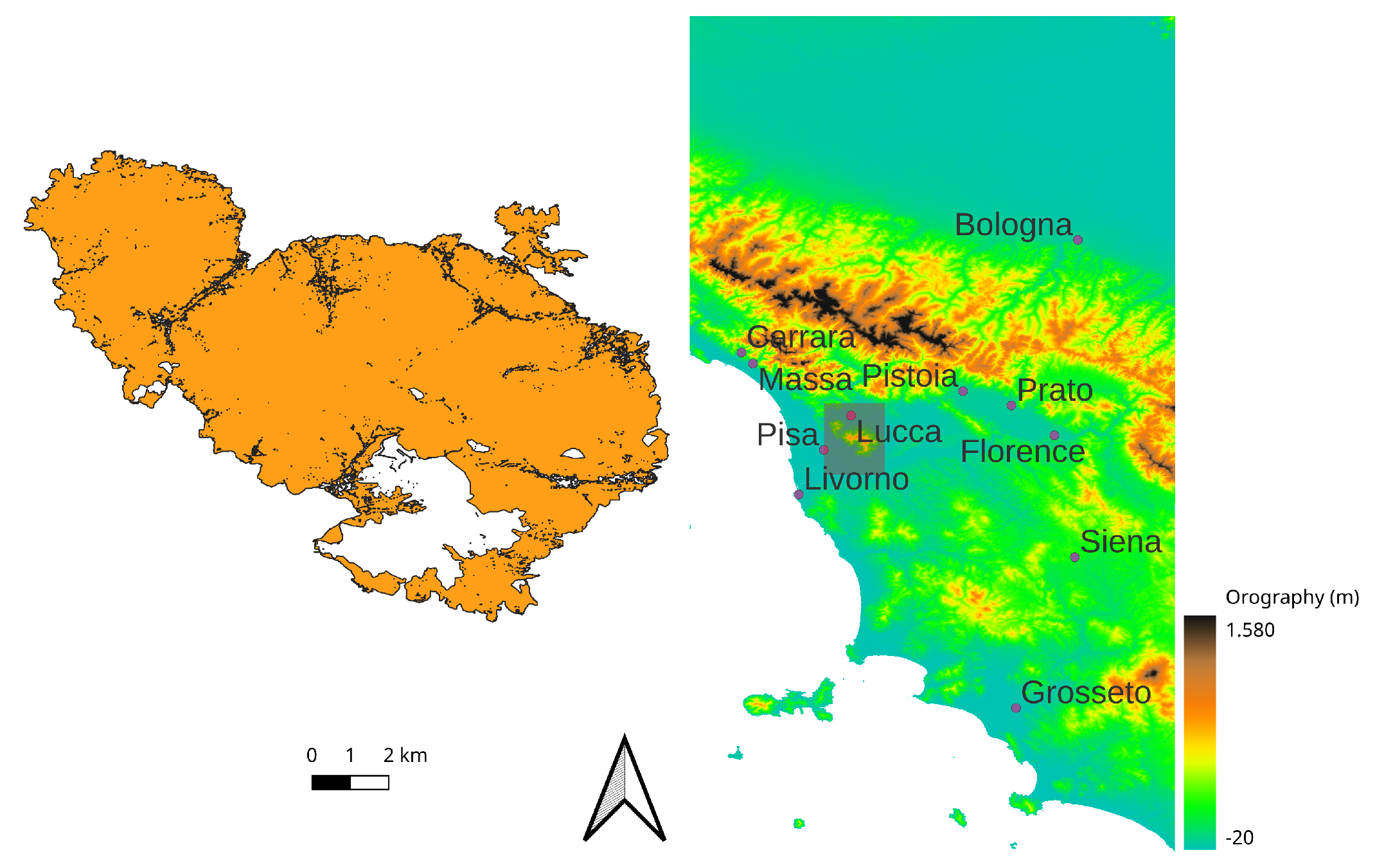
Figure A2.
Workflow of the MULTI and SINGLE experiment.
References
- Wulder, M. A.; Dechka, J. A.; Gillis, M. A.; Luther, J. E.; Hall, R. J.; Beaudoin, A.; Franklin, S. E. Operational mapping of the land cover of the forested area of Canada with Landsat data: EOSD land cover program. For. Chron. 2003, 79, 1075–1083. [Google Scholar] [CrossRef]
- Wulder, M. A.; Coops, N. C.; Roy, D. P.; White, J. C.; Hermosilla, T. Land cover 2.0. Int. J. Remote Sens. 2018, 39, 4254–4284. [Google Scholar] [CrossRef]
- Keshtkar, H.; Voigt, W.; Alizadeh, E. . Land-Cover Classification And Analysis Of Change Using Machine-Learning Classifiers And Multi-Temporal Remote Sensing Imagery. Arab. J. Geosci. 2017, 10. [Google Scholar] [CrossRef]
- Nagendra, H.; Reyers, B.; Lavorel, S. Impacts of land change on biodiversity: making the link to ecosystem services. Curr. Opin. Environ. Sustain. [CrossRef]
- Álvarez-Martínez, J.M.; Jiménez-Alfaro, B.; Barquín, J. , et al. Modelling the area of occupancy of habitat types with remote sensing. Methods Ecol. Evol. 2018, 9, 580–593. [Google Scholar] [CrossRef]
- Mücher, C. A.; Hennekens, S. M.; Bunce, R. G.; Schaminée, J. H.; Schaepman, M. E. Modelling the spatial distribution of Natura 2000 habitats across Europe. Landsc. Urban Plan. 2009, 2009 92, 148–159. [Google Scholar] [CrossRef]
- Roelofsen, H. D.; Peter; Kooistra, L. ; Witte, J.-P. M. Predicting Leaf Traits of Herbaceous Species from Their Spectral Characteristics. Ecol. Evol. 2014, 4, 706–719. [Google Scholar] [CrossRef]
- Sittaro, F.; Hutengs, C.; Semella, S.; Vohland, M. A Machine Learning Framework for the Classification of Natura 2000 Habitat Types at Large Spatial Scales Using MODIS Surface Reflectance Data. Remote Sens. 2022, 14, 823. [Google Scholar] [CrossRef]
- Bringezu, S.; Potočnik, J.; Schandl, H.; Lu, Y.; Ramaswami, A.; Swilling, M.; Suh, S. Multi-Scale Governance of Sustainable Natural Resource Use—Challenges and Opportunities for Monitoring and Institutional Development at the National and Global Level. Sustainability 2016, 8, 778. [Google Scholar] [CrossRef]
- Panuju, D. R.; Paull, D. J.; Griffin, A. L. Change detection techniques based on multispectral images for investigating land cover dynamics. Remote Sens. 2020, 12, 1781. [Google Scholar] [CrossRef]
- Eigenbrod, F.; Gonzalez, P.; Dash, J.; Steyl, I. Vulnerability of ecosystems to climate change moderated by habitat intactness. Glob. Chang. Biol. 2015, 21, 275–286. [Google Scholar] [CrossRef]
- Huang, Z.; Cao, C.; Chen, W.; Xu, M.; Dang, Y.; Singh, R.P.; Bashir, B.; Xie, B.; Lin, X. Remote Sensing Monitoring of Vegetation Dynamic Changes after Fire in the Greater Hinggan Mountain Area: The Algorithm and Application for Eliminating Phenological Impacts. Remote Sens. 2020, 12, 156. [Google Scholar] [CrossRef]
- Schiller, C.; Költzow, J.; Schwarz, S.; Schiefer, F.; Fassnacht, F.E. Forest Disturbance Detection in Central Europe Using Transformers and Sentinel-2 Time Series. Remote Sens. Environ. 2024, 315, 114475. [Google Scholar] [CrossRef]
- Peerbhay, K. Y.; Mutanga, O.; R. Ismail, R. Random Forests Unsupervised Classification: The Detection and Mapping of Solanum mauritianum Infestations in Plantation Forestry Using Hyperspectral Data. IEEE J. Sel. Top. Appl. Earth Obs. Remote Sens. 2015, 8, 3107–3122. [Google Scholar] [CrossRef]
- Malinowski, R.; Lewiński, S.; Rybicki, M.; Gromny, E.; Jenerowicz, M.; Krupiński, M.; Nowakowski, A.; Wojtkowski, C.; Krupiński, M.; Krätzschmar, E.; et al. Automated Production of a Land Cover/Use Map of Europe Based on Sentinel-2 Imagery. Remote Sens. 2020, 12, 3523. [Google Scholar] [CrossRef]
- Foley, J. A.; et al. Global Consequences of Land Use. Science 2005, 309, 570–574. [Google Scholar] [CrossRef]
- Wulder, M. A.; Hermosilla, T.; Stinson, G.; Gougeon, F. A.; White, J. C.; Hill, D. A.; Smiley, B. P. . Satellite-based time series land cover and change information to map forest area consistent with national and international reporting requirements. Forestry 2020, 2020 93, 331–343. [Google Scholar] [CrossRef]
- Ignatius, A.R.; Annis, A.N.; Helton, C.A.; Reeb, A.W.; Ricke, D.F. Spatiotemporal Vegetation Dynamics, Forest Loss, and Recovery: Multidecadal Analysis of the U.S. Triple Crown National Scenic Trail Network. Remote Sens. 2025, 17, 1142. [Google Scholar] [CrossRef]
- Zhang, X.; Zhao, T.; Xu, H.; Liu, W.; Wang, J.; Chen, X.; Liu, L. GLC_FCS30D: the first global 30 m land-cover dynamics monitoring product with a fine classification system for the period from 1985 to 2022 generated using dense-time-series Landsat imagery and the continuous change-detection method. Earth Syst. Sci. Data 2024, 16, 1353–1381. [Google Scholar] [CrossRef]
- Gavish, Y.; O’Connell, J.; Marsh, C.J.; Tarantino, C.; Blonda, P.; Tomaselli, V.; Kunin, W.E. Comparing the performance of flat and hierarchical habitat/land-cover classification models in a NATURA 2000 site. ISPRS J. Photogramm. Remote Sens. 2017, 136, 1–12. [Google Scholar] [CrossRef]
- Foody, G.M. Status of land cover classification accuracy assessment. Remote Sens. Environ. 2002, 80, 185–201. [Google Scholar] [CrossRef]
- Manandhar, R.; Odeh, I.O.A.; Ancev, T. Improving the Accuracy of Land Use and Land Cover Classification of Landsat Data Using Post-Classification Enhancement. Remote Sens. 2009, 1, 330–344. [Google Scholar] [CrossRef]
- Stehman, S.V.; Foody, G.M. Key issues in rigorous accuracy assessment of land cover products. Remote Sens. Environ. 2019, 231, 111199. [Google Scholar] [CrossRef]
- Olofsson, P.; Foody, G.M.; Herold, M.; Stehman, S.V.; Woodcock, C.E.; Wulder, M.A. Good practices for estimating area and assessing accuracy of land change. Remote Sens. Environ. 2014, 148, 42–57. [Google Scholar] [CrossRef]
- Gómez, C.; White, J.C.; Wulder, M.A. Optical Remotely Sensed Time Series Data for Land Cover Classification: A Review. ISPRS J. Photogramm. Remote Sens. 2016, 116, 55–72. [Google Scholar] [CrossRef]
- Franklin, S. E.; Ahmed, O. S.; Wulder, M. A.; White, J. C.; Hermosilla, T.; Coops, N. C. Large Area Mapping of Annual Land Cover Dynamics Using Multitemporal Change Detection and Classification of Landsat Time Series Data. Can. J. Remote Sens. 2015, 41, 293–314. [Google Scholar] [CrossRef]
- Pouliot, D.; Latifovic, R.; Zabcic, N.; Guindon, L.; Olthof, I. Development and Assessment of a 250 m Spatial Resolution MODIS Annual Land Cover Time Series (2000–2011) for the Forest Region of Canada Derived from Change-Based Updating. Remote Sens. Environ. 2014, 140, 73–743. [Google Scholar] [CrossRef]
- Bertacchi, A.; Sani, A.; Tomei, P.E. La Vegetazione del Monte Pisano. Felici Ed., Pisa, 2004.
- Gennai-Schott, S.; Sabbatini, T.; Rizzo, D.; Marraccini, E. Who Remains When Professional Farmers Give Up? Some Insights on Hobby Farming in an Olive Groves-Oriented Terraced Mediterranean Area. Land 2020, 9, 168. [Google Scholar] [CrossRef]
- Immitzer, M.; Neuwirth, M.; Böck, S.; Brenner, H.; Vuolo, F.; Atzberger, C. Optimal Input Features for Tree Species Classification in Central Europe Based on Multi-Temporal Sentinel-2 Data. Remote Sens. 2019, 11, 2599. [Google Scholar] [CrossRef]
- Descombes, P.; Walthert, L.; Baltensweiler, A.; Meuli, R.G.; Karger, D.N.; Ginzler, C.; Ginzler, G.; Zimmermann, N.E. Spatial modelling of ecological indicator values improves predictions of plant distributions in complex landscapes. Ecography 2020, 43, 1448–1463. [Google Scholar] [CrossRef]
- Italian Shoreline and River Network. Available online: http://www.pcn.minambiente.it/mattm/servizio-di-scaricamento-wfs/ (accessed on 22 October 2024).
- Digital Elevation Model of Italy at 20 m Spatial Resolution. Available online: http://www.sinanet.isprambiente.it/it/sia-ispra/download-mais/dem20/view (accessed on 22 October 2024).
- Braca, G.; Ducci, D. Development of a GIS based procedure (BIGBANG 1.0) for evaluating groundwater balances at National scale and comparison with groundwater resources evaluation at local scale. In Groundwater and Global Change in the Western Mediterranean Area, 53–61, 2018. Springer International Publishing.
- Fioravanti, G.; Toreti, A.; Fraschetti, P.; Perconti, W.; Desiato, F. Gridded monthly temperatures over Italy. In Proceedings of the 10th EMS Annual Meeting, Zürich, Switzerland, 13–17 September 2010; p. EMS2010-306.
- Duveiller, G.; Filipponi, F.; Ceglar, A. et al. Revealing the widespread potential of forests to increase low-level cloud cover. Nat. Commun. 2021, 2021 12, 4337. [Google Scholar] [CrossRef]
- Karsten, F.; Czeplak, G. Solar terrestrial radiation dependent on the amount and type of clouds. Sol. Energy 1980, 24, 177–189. [Google Scholar] [CrossRef]
- SoilGrids—global gridded soil information https://www.isric.org/explore/soilgrids, accessed on 28 April 2025.
- Szantoi, Z.; Strobl, P. . Copernicus Sentinel-2 Calibration and Validation. Europ. J. Remote Sens. 2019; 52, 253–255. [Google Scholar] [CrossRef]
- Phiri, D.; Simwanda, M.; Salekin, S.; Nyirenda, V.R.; Murayama, Y.; Ranagalage, M. Sentinel-2 Data for Land Cover/Use Mapping: A Review. Remote Sens. 2020, 12, 2291. [Google Scholar] [CrossRef]
- Moritz, S.; Bartz-Beielstein, T. ImputeTS: Time Series Missing Value Imputation in R. The R Journal 2017, 9, 207–218. [Google Scholar] [CrossRef]
- Agrillo, E.; Filipponi, F.; Pezzarossa, A.; Casella, L.; Smiraglia, D.; Orasi, A.; Attorre, F.; Taramelli, A. Earth Observation and Biodiversity Big Data for Forest Habitat Types Classification and Mapping. Remote Sens. 2021, 13, 1231. [Google Scholar] [CrossRef]
- Huete, A.; Justice, C.; Liu, H. Development of vegetation and soil indices for MODIS-EOS. Remote Sens. Environ. 1994, 49, 224–234. [Google Scholar] [CrossRef]
- Sulik, J.J. , Long, D.S. Spectral considerations for modeling yield of canola. Remote Sens. Environ. 2016, 184, 161–174. [Google Scholar] [CrossRef]
- Escadafal, R.; Huete, A. Improvement in remote sensing of low vegetation cover in arid regions by correcting vegetation indices for soil “noise” (Etude des proprieties spectrales des sols arides appliquee a l’amelioration des indices de vegetation obtenus par teledetection). Acad. Sci. Comptes Rendus Ser. II Mec. Phys. Chim. Sci. Terre l’Univers 1991, 312, 1385–1391. [Google Scholar]
- Gitelson, A. A.; Zur, Y.; Chivkunova, O. B.; Merzlyak, M. N. Assessing carotenoid content in plant leaves with reflectance spectroscopy. Photochem. Photobiol. 2002, 75, 272–281. [Google Scholar] [CrossRef]
- Wright, M. N.; Ziegler, A. (2017). ranger: A Fast Implementation of Random Forests for High Dimensional Data in C++ and R. J. Stat. Softw. 2017, 77, 1–17. [Google Scholar] [CrossRef]
- Breiman, L. Random forests. Mach. Learn. 2001, 45, 5–32. [Google Scholar] [CrossRef]
- Geurts, P.; Ernst, D.; Wehenkel, L. Extremely randomized trees. Mach. Learn. 2006, 63, 3–42. [Google Scholar] [CrossRef]
- Meinshausen, N. Quantile Regression Forests. J. Mach. Learn. Res. 2006 7 983–999. http://www.jmlr.org/papers/v7/meinshausen06a.html.
- Dormann, C.F.; Elith, J.; et al. Collinearity: a review of methods to deal with it and a simulation study evaluating their performance. Ecography 2023, 36, 27–46. [Google Scholar] [CrossRef]
- Plourde, L.; Congalton, R.G. Sampling method and sample placement: How do they affect the accuracy of remotely sensed maps? Photogrammet. Eng. Remote Sens. 2003, 69, 289–297. [Google Scholar] [CrossRef]
- Stehman, S.V. Practical Implications of Design-Based Sampling Inference for Thematic Map Accuracy Assessment. Remote Sens. Environ. 2000, 72, 35–45. [Google Scholar] [CrossRef]
- Story, M.; Congalton, R.G. Accuracy Assessment—A Users Perspective. Photogrammetr. Eng. Remote Sens. 1986, 52, 397–399. [Google Scholar]
- Olofsson, P.; Foody, G.M.; Stehman, S.V.; Woodcock, C.E. Making better use of accuracy data in land change studies: Estimating accuracy and area and quantifying uncertainty using stratified estimation. Remote Sens. Environ. 2013, 129, 122–131. [Google Scholar] [CrossRef]
- Brown, C.E. Coefficient of Variation. In: Applied Multivariate Statistics in Geohydrology and Related Sciences. Springer, Berlin, Heidelberg. 1998. [CrossRef]
- Cochran, W. G. Sampling techniques. 1997. New York, NY: Wiley.
- Li, C.; Ma, Z.; Wang, L.; Yu, W.; Tan, D.; Gao, B.; Feng, Q.; Guo, H.; Zhao, Y. Improving the Accuracy of Land Cover Mapping by Distributing Training Samples. Remote Sens. 2021, 4594. [Google Scholar] [CrossRef]
- Vali, A.; Comai, S.; Matteucci, M. Deep Learning for Land Use and Land Cover Classification Based on Hyperspectral and Multispectral Earth Observation Data: A Review. Remote Sens. 2020, 12, 2495. [Google Scholar] [CrossRef]
- Zhao, Y.; Feng, D.; Yu, L.; Wang, X.; Chen, Y.; Bai, Y.; Hernández, H.J.; Galleguillos, M.; Estades, C.; Biging, G.S.; et al. Detailed dynamic land cover mapping of Chile: Accuracy improvement by integrating multi-temporal data. Remote Sens. Environ. 2016, 183, 170–185. [Google Scholar] [CrossRef]
- Zhao, Y.; Feng, D.; Yu, L.; Cheng, Y.; Zhang, M.; Liu, X.; Xu, Y.; Fang, L.; Zhu, Z.; Gong, P. Long-term land cover dynamics (1986–2016) of Northeast China derived from a multi-temporal landsat archive. Remote Sens. 2019, 11, 599. [Google Scholar] [CrossRef]
- Campelo, F.; Rubio-Cuadrado, Á.; Montes, F.; Colangelo, M.; Valeriano, C.; Camarero, J. J. Growth phenology adjusts to seasonal changes in water availability in coexisting evergreen and deciduous mediterranean oaks. For. Ecosys. 2023, 10, 100134. [Google Scholar] [CrossRef]
- Lionello, P.; Malanotte-Rizzoli, P.; Boscolo, R.; Alpert, P.; Artale, V.; Li, L.; Luterbacher, J.; May, W.; Trigo, R.; Tsimplis, M.; et al. The Mediterranean climate: An overview of the main characteristics and issues, Mediterranean Climate Variability. Dev. Earth Environ. Sci. 2006, 4, 1–26. [Google Scholar]
- Sinha, P.; Kumar, L.; Reid, N. Seasonal Variation in Land-Cover Classification Accuracy in a Diverse Region. Photogramm. Eng. Remote Sens. 2012, 78, 271–280. [Google Scholar] [CrossRef]
- Praticó, S.; Solano, F.; Di Fazio, S.; Modica, G. Machine Learning Classification of Mediterranean Forest Habitats in Google Earth Engine Based on Seasonal Sentinel-2 Time-Series and Input Image Composition Optimisation. Remote Sens. 2021, 13, 586. [Google Scholar] [CrossRef]
- Ulsig, L.; Nichol, C.J.; Huemmrich, K.F.; Landis, D.R.; Middleton, E.M.; Lyapustin, A.I.; Mammarella, I.; Levula, J.; Porcar-Castell, A. Detecting Inter-Annual Variations in the Phenology of Evergreen Conifers Using Long-Term MODIS Vegetation Index Time Series. Remote Sens. 2017, 9, 49. [Google Scholar] [CrossRef]
- Misra, G.; Cawkwell, F.; Wingler, A. Status of Phenological Research Using Sentinel-2 Data: A Review. Remote Sens. 2020, 12, 2760. [Google Scholar] [CrossRef]
Figure 1.
Region of Interest: Monti Pisani massif, without the burned areas from 2001 onward and targets lying in the ROI with the specified classes
Figure 1.
Region of Interest: Monti Pisani massif, without the burned areas from 2001 onward and targets lying in the ROI with the specified classes
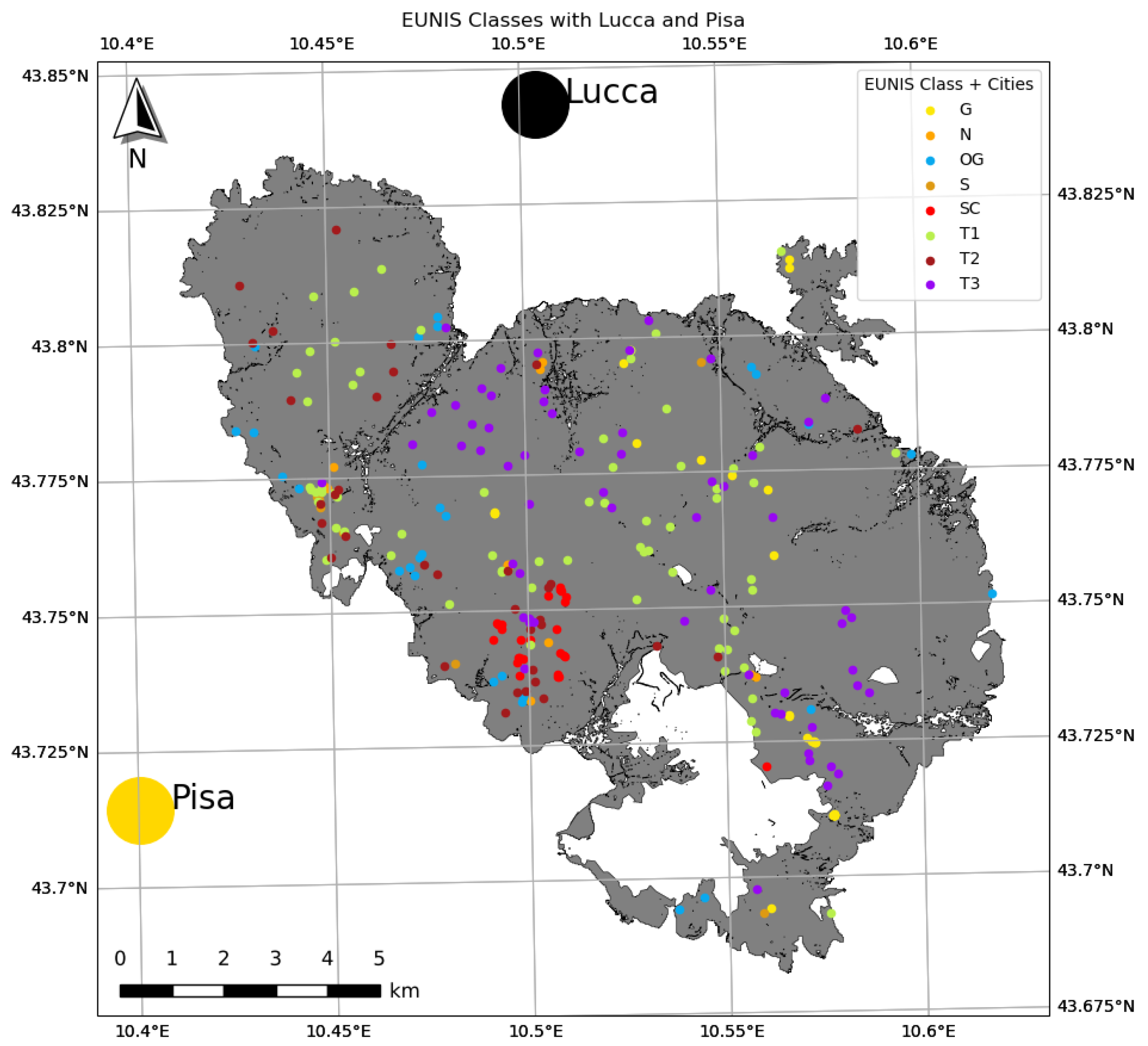
Figure 2.
Modal value of classified classes for the MULTI (a) and SINGLE (b) experiments
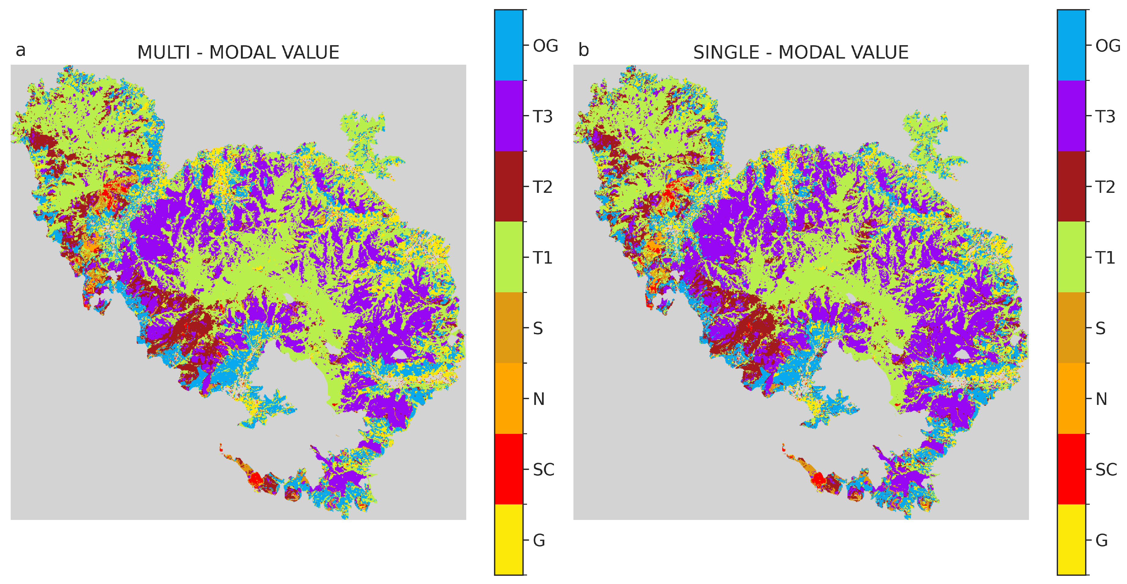
Figure 3.
Spatial distribution where the two modal values shown in Figure 2 differ
Figure 3.
Spatial distribution where the two modal values shown in Figure 2 differ
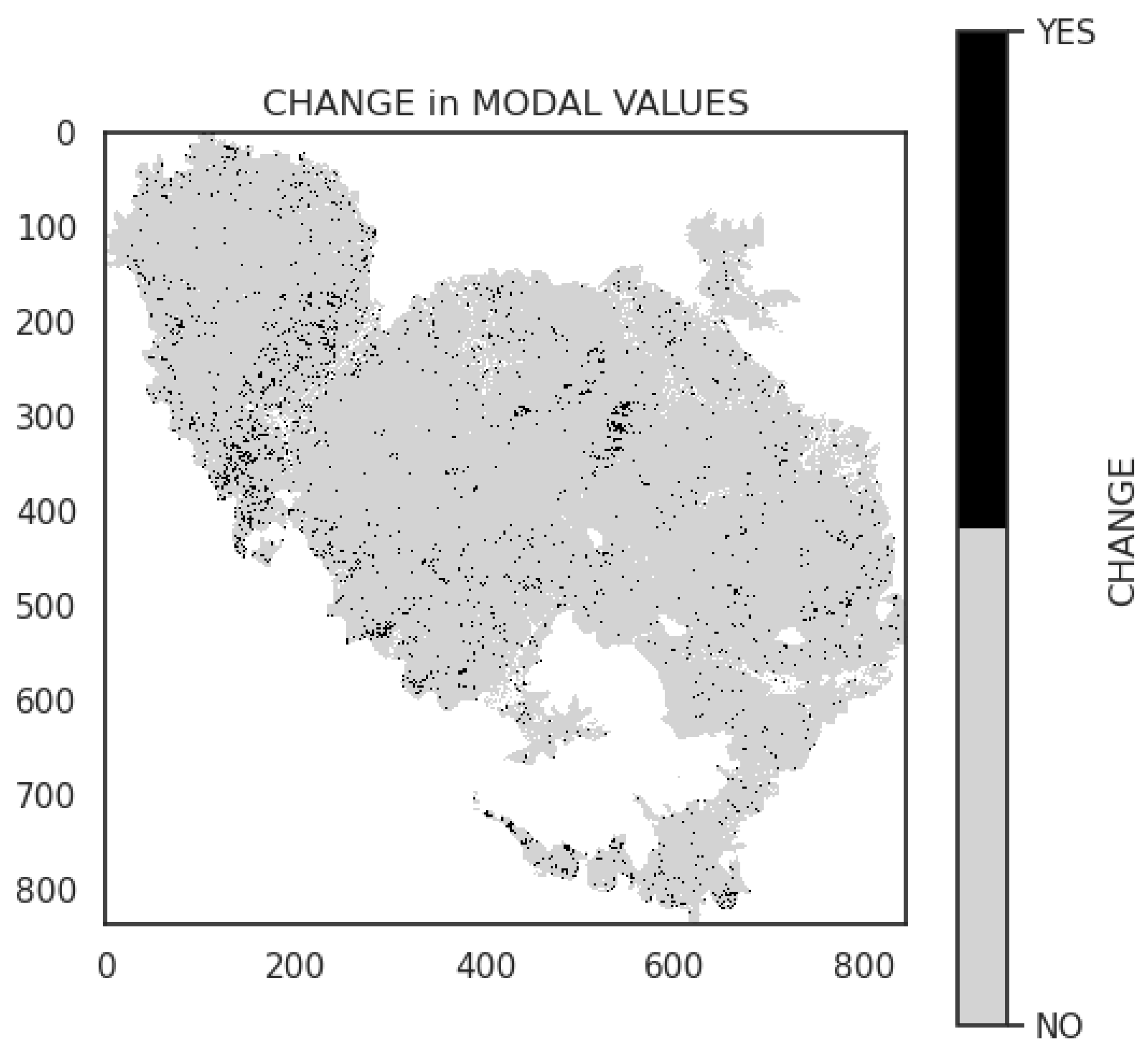
Figure 4.
Pixel stability for the MULTI (a) and SINGLE (b) experiments
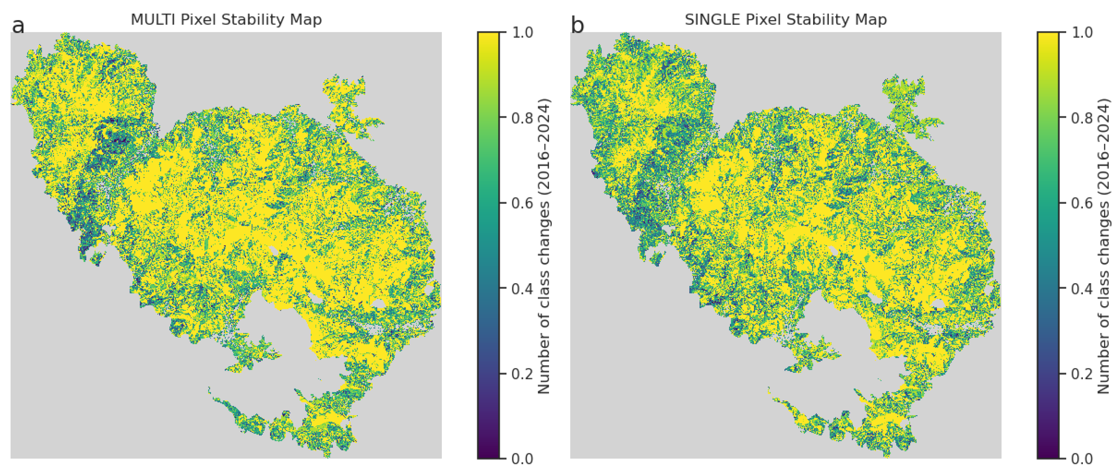
Figure 5.
The solid line represents the spatial average, while the shadow indicates the standard deviation of the observed Band 8 values in April for various classes.
Figure 5.
The solid line represents the spatial average, while the shadow indicates the standard deviation of the observed Band 8 values in April for various classes.
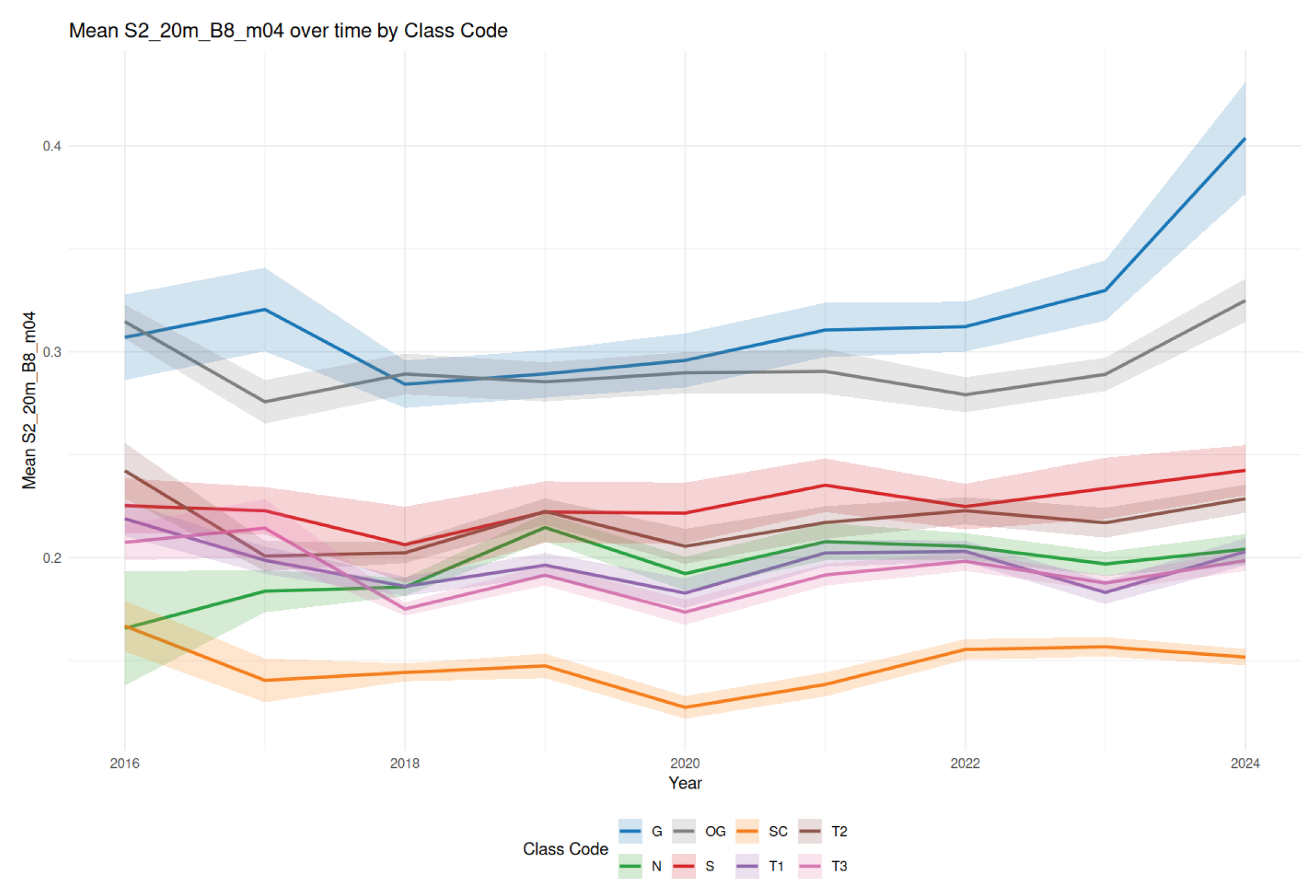
Table 1.
Number of plots for each class.
| G | SC | N | S | T1 | T2 | T3 | OG | |
| N plots | 31 | 26 | 16 | 27 | 82 | 47 | 71 | 29 |
Table 2.
Definition of spectral indexes used as predictors and their references.
| Spectral Index | Equation | Reference |
| Enhanced Vegetation Index EVI | [43] | |
| Normalized Difference Yellow Index NDYI | [44] | |
| Normalized Difference Red/Green Redness Index RI | [45] | |
| Carotenoid Reflectance Index CRI1 | [46] |
Table 3.
statistics of mapped areas (in ha) for the eight classes for both the experiments.
| G | SC | N | S | T1 | T2 | T3 | OG | ||
| MULTI | AVERAGE | 1260.0 | 162.0 | 55.9 | 287.0 | 4969.6 | 1281.6 | 3332.3 | 1822.7 |
| STDEV | 209.6 | 117.9 | 9.1 | 139.1 | 112.3 | 220.4 | 143.9 | 277.8 | |
| CV | 0.17 | 0.73 | 0.16 | 0.48 | 0.02 | 0.17 | 0.04 | 0.15 | |
| SINGLE | AVERAGE | 1034.2 | 184.6 | 60.5 | 269.0 | 4464.9 | 1573.3 | 3518.1 | 2066.5 |
| STDEV | 86.3 | 75.8 | 19.0 | 67.7 | 586.1 | 433.3 | 359.7 | 466.2 | |
| CV | 0.08 | 0.41 | 0.31 | 0.25 | 0.13 | 0.28 | 0.10 | 0.23 |
Disclaimer/Publisher’s Note: The statements, opinions and data contained in all publications are solely those of the individual author(s) and contributor(s) and not of MDPI and/or the editor(s). MDPI and/or the editor(s) disclaim responsibility for any injury to people or property resulting from any ideas, methods, instructions or products referred to in the content. |
© 2025 by the authors. Licensee MDPI, Basel, Switzerland. This article is an open access article distributed under the terms and conditions of the Creative Commons Attribution (CC BY) license (http://creativecommons.org/licenses/by/4.0/).
Copyright: This open access article is published under a Creative Commons CC BY 4.0 license, which permit the free download, distribution, and reuse, provided that the author and preprint are cited in any reuse.


