Submitted:
21 May 2025
Posted:
21 May 2025
You are already at the latest version
Abstract
Ground-based cloud detection remains challenging due to the cloud morphological complexity, inter-class visual ambiguity, and dynamic background interference. Although deep learning has enhanced detection precision, conventional random sampling training paradigms overlook the heterogeneous spectrum of cloud sample difficulty levels. This paper proposes CurriCloud, a dynamic curriculum learning framework that automatically adapts to cloud detection challenges through two key innovations: (1) a loss-adaptive difficulty measurement approach that evaluates sample complexity in real-time based on training performance, and (2) a phase-wise threshold scheduling mechanism that progressively adjusts sample selection to match the model’s capability. Extensive experiments on the ALPACLOUD benchmark demonstrate CurriCloud’s effectiveness across diverse architectures including YOLOv10s, SSD, and RT-DETR-R50, compared with random sampling training paradigms. Ablation studies demonstrate CurriCloud’s robustness to hyperparameter variations, while comparative analyses show superior precision-recall balance over static curriculum methods. The architecture-agnostic design enables seamless integration with CNNs and transformers, offering practical value for meteorological observation systems.
Keywords:
cloud object detection
; curriculum learning
; unified loss function
; loss adaptive curriculum scheduling
1. Introduction
Ground-based cloud detection, as a core component of meteorological observation systems, plays a crucial role in analyzing weather transitions and multi-domain meteorological services [1,2,3].
Different types of clouds indicate distinct weather changes. For instance, mammatus clouds are often associated with hail or extreme weather events, while Altocumulus lenticularis clouds signal strong wind shear and a high risk of aviation turbulence. Therefore, real-time, high-precision ground-based cloud detection is essential for localized short-term extreme weather warnings. Additionally, ground-based cloud detection is vital in photovoltaic power generation forecasting [4]. The movement and morphological changes of clouds directly influence solar radiation intensity distribution, thereby affecting the efficiency of photovoltaic power plants. Ground-based cloud monitoring systems can accurately capture the spatiotemporal characteristics of clouds, optimizing photovoltaic power prediction models and reducing intermittent fluctuations in power output. Compared to satellite observations, ground-based imaging systems provide higher-resolution cloud data, compensating for the lack of spatiotemporal detail in satellite observations and offering richer information for meteorological research and applications.
However, ground-based cloud detection faces numerous technical challenges. First, cloud morphology exhibits high diversity and complexity [5], as illustrated in Figure 1 [6]. Different cloud categories may share similar visual features. For example, opaque altostratus and nimbostratus clouds are often indistinguishable to untrained observers. Second, clouds and certain surface features (e.g., deserts, snow-covered terrain) exhibit spectral similarities, increasing the risk of false detection. Furthermore, the presence of occlusion effects in multi-layer cloud systems leads to boundary ambiguity, significantly complicating detection.
These challenges limit the effectiveness of traditional machine learning methods based on handcrafted features [7,8,9]. In recent years, deep learning techniques, particularly convolutional neural networks (CNNs) and Transformer architectures, have achieved remarkable progress in object detection [10,11,12,13,14] However, directly applying generic detection models(e.g., YOLO series [10], SSD [13], and RT-DETR [15]) to cloud detection tasks may yield limited performance due to training (source) domain bias and unique physical properties of clouds. Some studies have attempted to improve performance through model refinement or transfer learning [16,17,18,19], yet conventional random sampling training paradigms overlook the inherent variability in sample difficulty, neglecting its impact on model learning.This may lead to limited generalization in complex scenarios and fails to address issues such as misclassification and false detection. The complexity of cloud morphology, inter-class visual similarity, and dynamic background interference remain major challenges in current research.
Curriculum Learning (CL) [20], a machine learning paradigm inspired by human education, first introduced by Bengio et al. and validated both theoretically and empirically. Its fundamental premise involves progressively training models from simple to complex samples to improve learning efficiency and final performance. CL operates on three key principles: (1) quantifiable difficulty differences among samples, where easier examples enable faster development of effective feature representations; (2) knowledge accumulation, where simple features form foundations for learning complex patterns; and (3) dynamic adaptation, where optimal learning progression adjusts based on real-time model performance to optimize neural network parameter exploration [20].
These principles naturally align with CNN’s hierarchical feature extraction and the multidimensional challenges in cloud detection. While CL has demonstrated success across computer vision domains [21,22], its application to cloud detection remains underexplored To address this gap, we propose CurriCloud, a loss-adaptive curriculum learning framework specifically designed for ground-based cloud detection, which dynamically adjusts training sample difficulty and optimizes progressive training. The core innovations of this framework include: (1) A loss-adaptive difficulty measurementthat automatically evaluates sample complexity based on real-time training performance; (2) A phase-wise threshold schedulingmechanism that progressively adjusts training sample selection to match the model’s evolving capability; and (3)A network-agnostic design compatible with both CNN- and Transformer-based detectors, automatically tailoring the curriculum to each architecture’s learning characteristics.
The main contributions of this work can be summarized as follows:
(1) A dynamic curriculum learning framework specifically designed for ground-based cloud detection is proposed, where detection performance is significantly improved through adaptive difficulty assessment and phase-wise training optimization. To the best of our knowledge, this represents the first implementation of adaptive curriculum learning explicitly tailored for cloud detection tasks.
(2) A general loss-adaptive difficulty measurement method is designed, where reliance on manual difficulty annotation is eliminated, providing a novel approach for applying curriculum learning in remote sensing applications.
(3) Unlike all-sky cloud images or pure-sky cloud images, we constructed ALPACLOUD, a ground-based cloud image dataset with diverse ground backgrounds, better reflecting real-world scenarios and improving the model’s robustness against background interference.
(4) Comprehensive experiments are conducted on the ALPACLOUD dataset, where the effectiveness and robustness of CurriCloud across different detection architectures are validated. Differentiated optimization patterns of CurriCloud’s core hyperparameters are revealed. Additionally, CurriCloud is compared with Static CL, a static curriculum learning scheme with predefined sample difficulty, where the superiority of the dynamic curriculum learning approach is confirmed by outperforming CurriCloud-SL on most metrics.
2. Related Works
2.1. Ground- Based Cloud Detection
Recent years have witnessed remarkable progress in ground-based cloud analysis through deep learning approaches [23,24]. The field has evolved along two main directions: cloud classification and cloud detection. For classification tasks, seminal works include CloudA [25]which established the first dedicated CNN architecture, TGCN [26] that introduced graph convolutional networks to model spatial relationships between cloud formations, and subsequent improvements addressing specific challenges like intra-class variation and occlusion robustness [24]. Parallel developments in transfer learning extended these methods to data-scarce scenarios [18,19].
While these classification methods have significantly advanced cloud analysis, operational meteorological applications increasingly demand real-time systems capable of simultaneously localizing and classifying clouds. Modern detection frameworks have demonstrated exceptional potential in this regard: the YOLO series [11], with its efficient single-stage architecture, delivers remarkable inference speeds on modern GPUs while maintaining competitive accuracy - making it ideal for real-time sky monitoring; while DETR’s [14,15]end-to-end transformer approach eliminates traditional components like anchor boxes and non-maximum suppression, particularly suitable for occluded and overlapping cloud scenarios. However, applying these generic detectors to cloud analysis requires significant adaptations due to unique atmospheric characteristics. Recent advances have diversified to include domain-specific loss functions [16], YOLO architectures for multiscale detection [27], and DETR variants optimized for complex background interference [17,28], among other innovations. Despite these advances, current approaches share a fundamental limitation: they focus exclusively on architectural modifications while employing static training paradigms that cannot adapt to the varying difficulty of cloud samples.
This reveals a critical research gap - the need for dynamic training frameworks that address cloud-specific challenges during learning. Our work bridges this gap through a novel curriculum learning approach that maintains architectural generality while achieving comprehensive performance improvements via intelligent, physics-aware training sample selection and difficulty adjustment.
2.2. Loss Functions for Object Detection
The performance of detection models hinges critically on the design of loss functions, which must simultaneously optimize localization accuracy (i.e., bounding box regression) and classification confidence while balancing gradient contributions across subtasks. Modern detection losses typically integrate three key components:
(1) Classification Loss: This measures the discrepancy between predicted and ground-truth class labels. Widely adopted variants include Cross-Entropy (CE) loss and Focal Loss [29].
(2) Localization Loss: This quantifies spatial deviations between predicted and ground-truth bounding boxes. Early frameworks relied on L1/L2, or Smooth L1 norms [30], while recent advancements introduced Intersection over Union (IoU) based losses such as GIoU [31] and GCIoU [32].
(3) Auxiliary Losses: Advanced frameworks incorporate domain-specific constraints. For example, YOLOv10 [12] employs Distribution Focal Loss (DFL) to model bounding box distribution statistics, enhancing robustness in detecting irregular geological features.
Existing loss functions are tightly coupled with detector architectures—anchor-free methods like FCOS [33] rely on auxiliary center-ness losses, while Transformer-based detectors (e.g., RT-DETR) require Hungarian matching for prediction deduplication. This architectural dependency limits cross-framework adaptability and complicates optimization for specialized tasks such as cloud detection. Our work proposes an architecture-agnostic unified loss that decouples from specific detection paradigms, including both CNN- and Transformer-based approaches.
2.3. Curriculum Learning
A general framework for CL design consists of these two core components: (1)difficulty measurer, which decides the relative easiness of each data example, and (2) a training scheduler, which decides the sequence of data subsets throughout the training process based on the judgment from the difficulty measurer [20]. Based on sample difficulty measurer methods, CL can be categorized into static and dynamic paradigms. The static paradigm pre-defines sample difficulty using specific metrics before training and maintains fixed difficulty levels throughout [20,34,35]. Recent developments have shifted toward dynamic paradigm that continuously adjusts sample difficulty according to the model’s evolving learning capacity during training.
Notable dynamic approaches include: (1) Self-Paced Learning (SPL) [36], a set of approaches in which the model ranks the samples from easy to hard during training, based on its current progress. For example, the inputs with the smaller loss at a certain time during training are easier than the samples with higher loss; (2) Self-Paced Curriculum Learning (SPCL) [37,38], which takes into account both prior knowledge known before training and the learning progress during training. Compared to human education, SPCL is analogous to the “instructor-student-collaborative” learning mode, rather than “instructor-driven” in CL or “student-driven” in SPL; and (3) the LeRaC method which leverages the use of a different learning rate for each layer of a neural network, assigns higher learning rates to neural layers closer to the input, gradually decreasing the learning rates as the layers are placed farther away from the input [39].
3. The Proposed Method
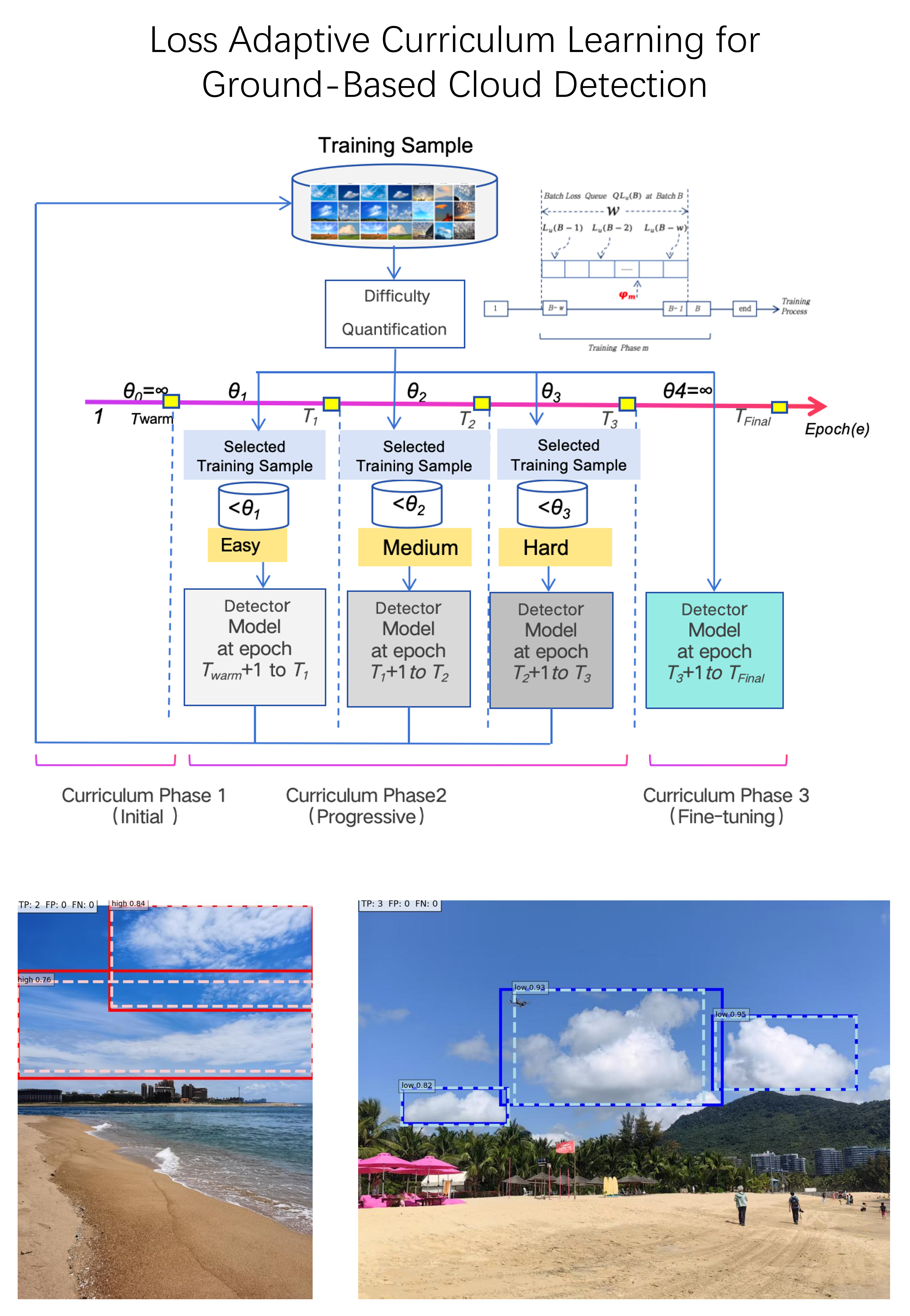
The proposed CurriCloud framework, as illustrated in Figure 2, is a novel curriculum learning-based approach designed to address the inherent challenges in ground-based cloud detection.
CurriCloud consists of two key components: real-time loss analysis and dynamic curriculum scheduling. Real-time loss analysis computes the current batch loss and maintains a loss sliding window queue to dynamically monitor training losses. It evaluates sample difficulty based on phase-specific adaptive thresholds without requiring manual annotations. The dynamic curriculum scheduling employs a phase-wise threshold mechanism to progressively adjust sample selection strategies according to the model’s evolving capabilities, enabling a step-by-step learning process from easy to hard cloud samples.
3.1. Loss Computing and Analysis
3.1.1. Unified Batch Loss
We propose a Unified Batch Loss (UBL) function that achieves architecture independence while effectively combining classification, localization, and auxiliary losses. This composite loss serves as a dynamic difficulty metric for batch evaluation, automatically balancing contributions from multiple cloud detection subtasks.
The UBL framework demonstrates compatibility with mainstream detectors, encompassing both CNN-based architectures such as the YOLO series and SSD, as well as Transformer-based models including DETR and RT-DETR.
Let B denote a training batch of N samples. The total loss for the batch B is defined as Equation (1):
where is the classification loss, measuring the discrepancy between predicted and ground-truth cloud class labels; denotes the localization loss, which quantifies spatial deviations between predicted and ground-truth cloud bounding boxes; and represents auxiliary losses (whose specific functions vary across different object detectors). The task-balancing coefficients , , are weighting parameters that can be either fixed or dynamically adjusted during the training process. If no auxiliary tasks are present, defaults to 0.
The batch-averaged loss ensures stable gradients across diverse cloud samples, particularly critical for heterogeneous scenes such as mixed urban and rural background variations.
3.1.2. Loss Sliding Window Queue
The loss sliding window queue is used to monitor the training loss distribution in real-time. It maintains the most recent w batches of loss values relative to the current batch B, represented as , where is defined in Equation (2).
operates as a First-In-First-Out (FIFO) queue, where its elements are dynamically updated during training. Here, w represents the queue length, as illustrated in Figure 3.
The window size w is determined through three key considerations: for short-term fluctuation filtering, w = 10 effectively smooths anomalies from challenging samples; for pattern retention in slow-converging architectures, w = 20 preserves sufficient historical information; while the queue operations maintain computational efficiency compared to full-loss sorting approaches, where total training batches.
3.2. Dynamic Loss Threshold
The dynamic loss threshold determines whether to retain the current sample’s training results for backpropagation. It is computed based on the loss sliding window queue values of the current batch B and the loss threshold quantile corresponding to the training phase m (as illustrated in Figure 3), as expressed in Equation (3):
where represents the -quantile operator applied to . Backpropagation is performed when ; otherwise, the sample is reselected.
The design of incorporates two key features:
- Relative Difficulty Assessment: Unlike static thresholds, automatically adapts to the current state of the model. As performance improves, the threshold dynamically decreases following the downward shift of the loss distribution, maintaining an optimal challenge level.
- Architectural Adaptability: The framework naturally accommodates detectors with different convergence characteristics - identical values produce detector-specific thresholds that match individual optimization trajectories.
This adaptive threshold mechanism dynamically adjusts according to both the training phase and the loss window queue, ensuring optimal alignment between sample difficulty and the model’s evolving capability.
3.3. Loss-Based Dynamic Curriculum Learning Scheduling
CurriCloud dynamically schedules training samples using the loss window queue and the adaptive threshold .
CurriCloud adopts a three-phase training protocol: full-sample initialization (), dynamic curriculum scheduling () and full-sample fine-tuning (). Each phase m is formally defined as Equation (4):
where denotes the epoch range, represents the phase-specific quantile threshold for sample difficulty selection.
Phase (Full-sample Initialization) employs unfiltered training on the complete data set to establish the representations of the basic characteristics. During this stage, the model learns fundamental cloud characteristics - including texture patterns and morphological shapes - through exhaustive exposure to all available samples. This comprehensive initialization strategy actively mitigates potential sampling bias in early training stages by preventing premature filtering of challenging instances, thereby fostering robust feature embeddings that serve as the basis for subsequent curriculum learning phases.
Phase (Dynamic Curriculum Scheduling) is further divided into three sub-phases ( and ) with progressively increasing sample difficulty, i.e., . The scheduling protocol operates as follows: First, the unified batch loss is computed for the current batch B. The loss value is then compared against the dynamic threshold . If , the detection model parameters are updated via backpropagation; otherwise, the batch is resampled. Whether or not the model is updated, gets added to the sliding loss queue using FIFO. The protocol implements a phased difficulty progression. Phase employs low thresholds (e.g., ) to incorporate a wider spectrum of sample difficulties, thereby improving model generalization capabilities. Phase employs a moderate threshold (e.g., ) to enhance capability through intermediate samples; while phase applies a high threshold (e.g., ) to focus optimization on challenging cases.
Phase (Full Fine-tuning) reverts to random sampling across the entire training set, effectively eliminating potential bias introduced by the preceding curriculum learning stages. This final phase serves dual critical purposes: (1) it prevents overfitting that could result from prolonged exposure to filtered samples during the dynamic scheduling phase, and (2) facilitates global convergence by allowing the model to perform unrestricted optimization across all difficulty levels. The unfiltered training paradigm ensures comprehensive exploration of the parameter space, while maintaining the robust feature representations developed during earlier phases.
CurriCloud demonstrates three fundamental improvements over conventional approaches: (1) inherent noise robustness through loss distribution-based difficulty estimation; (2) architectural universality via UBL that bridges CNN-Transformer optimization gaps; and (3) meteorologically interpretable thresholds aligned with WMO standards—notably when , the system automatically focuses on cirrus fibratus differentiation, replicating expert training progression through its dynamic curriculum.
4. Experiments
To validate the effectiveness of the CurriCloud strategy, we conducted comprehensive evaluations using three representative detectors on our ALPACLOUD dataset: (1) YOLOv10s (https://github.com/THU-MIG/yolov10), representing modern CNN-based architectures with optimized gradient flow; (2) RT-DETR-R50 (https://github.com/lyuwenyu/ RT-DETR), exemplifying Transformer-based real-time detection; and (3) Ultra-Light-Fast-Generic-Face-Detector-1MB (ULFG-FD, https://github.com/Linzaer/Ultra-Light-Fast-Generic-Face-Detector-1MB/), an SSD-derived ultra-lightweight detector, highlighting anchor-based designs under extreme model compression. This selection spans the full spectrum of contemporary detection paradigms (CNNs, Transformers, and traditional single-shot detectors), enabling rigorous assessment of CurriCloud’s adaptive training across: (1) multi-scale feature fusion (YOLOv10s), (2) attention-based query mechanisms (RT-DETR-R50), and (3) predefined anchor box systems (ULFG-FD).
4.1. Datasets
We evaluate our method on the ALPACLOUD dataset, as illustrated in Figure 4. ALPACLOUD comprises 1786 high-resolution (1068×756 pixels) ground-based cloud images. These images consist of two parts: one part is captured by ground-based camera sensors across seven Chinese provinces including Beijing, Hainan, Guangdong, Fujian, Shandong, Hebei and Liaoning; the other part is sourced from meteorological databases. ALPACLOUD was partitioned into 70.89% training set, 6.94% validation set, and 22.17% test set to ensure a balanced distribution for model evaluation. The annotation process employed the LabelImg toolbox with rigorous quality control: connected homogeneous clouds without obstacle occlusion are treated as a single target if their bodies are continuous, and as two separate targets if their bodies are discontinuous.
Following WMO standards, the images are annotated with five cloud categories, as showcased in Figure 4: (1) High clouds (High, 37.07%), (2) Low clouds (Low, 46.14%), (3) Altocumulus translucidus (Ac tra, 5.94%), (4) Altocumulus lenticularis (Ac len, 5.38%), and (5) mammatus clouds (Ma, 5.49%). This composition ensures comprehensive coverage of cloud morphological variations while incorporating challenging ground backgrounds common in operational nowcasting scenarios.
The statistical distribution closely mirrors natural cloud-type occurrence patterns, with high and low clouds dominating in frequency. While specialized formations like Altocumulus translucidus, Altocumulus lenticularis, and mammatus clouds exhibit lower incidence rates, their inclusion significantly enhances model generalizability through spectral-spatial diversity infusion; this proves particularly critical for enhancing nowcasting accuracy of high-impact meteorological phenomena. Cloud Classification and Morphological Features are illustrated in Table 1.
4.2. Evaluation Metrics
In our work, we employ mAP50, Precision, Recall as the evaluation criterion to evaluate the detection performance of our method. Considering the fractal structure and fuzzy edges of cloud boundaries, these metrics are adaptively adjusted to accommodate the inherent uncertainties in cloud morphology. Precision and Recall are respectively defined in Equations (5) and (6):
where TP (True Positive) refers to the correctly detected cloud areas, both locations and categories. FP (False Positive) represents the background areas misclassified as cloud or the incorrect cloud category, FN (False Negative) indicates the undetected real cloud areas.
Based on Equations (5) and (6), we can obtain definitions for the Average Precision (AP) and Mean Average Precision (mAP), as shown in Equations (7)and (8):
AP (Average Precision) is the area under the Precision-Recall curve for a single class. It integrates precision across all recall levels.
The mAP50 (mean Average Precision at MAIoU=0.5) provides the average value of the AP for each category, with denoting the number of cloud types in the whole dataset, where MAIoU (meteorologically adaptive Intersection over Union) is defined as (9):
where is the predicted box, and is the ground truth box. Based on , we propose a meteorologically adaptive lenient-matching strategy that incorporates: (1) One-to-Many Matching where a single prediction box can contain multiple homogeneous ground truth (GT) clouds, with TP counts based on the number of valid prediction boxes; (2) Many-to-One Matching where multiple predictions can match to a single GT cloud, with only the first matched prediction counted as TP and subsequent matches not penalized as FP. Figure 5 shows examples of the calculation of the metrics.
As shown in Figure 5(a), when a prediction box encloses multiple cirrus GTs, each unmatched GT independently increments the TP count. Conversely, Figure 5(b) demonstrates that substructure detections within cumulus layers contribute only 1 TP without triggering FPs. This strategy preserves critical capabilities for tracking cloud system movements (via bounding box coordinates) while significantly relaxing boundary precision requirements, better aligning with meteorological operational needs.
4.3. Implementation Details
Our evaluation was conducted on the ALPACLOUD dataset using YOLOv10s (CNN-based), RT-DETR-R50 (Transformer-based), and ULFG-FD (anchor-based). All experiments were performed on a dedicated Ubuntu 22.04 workstation equipped with an NVIDIA GeForce RTX 4090 GPU and Intel Core i9-14900HX processor, utilizing Python 3.9.21 and CUDA 12.6 for accelerated computing. For each object detection model, CurriCloud sums the losses of all categories within each sample batch with equal weights and uses this value as the UBL.
CurriCloud settings for different detector models are illustrated in Table 2.
We employed stochastic gradient descent (SGD) optimization for YOLOv10s and ULFG-FD, adaptive moment estimation (Adam) for RT-DETR-R50, maintaining consistent optimizer choices between conventional and CurriCloud training regimes to ensure fair comparison.
4.4. Results
Comparative experimental results demonstrated that CurriCloud consistently outperformed conventional training methods in mAP50 performance metrics across all architectures. Sensitivity analyses of the loss window length (w) and loss threshold () yielded deployment-specific optimization guidelines.
Experimental results are presented in Table 3.
The experimental results demonstrate that CurriCloud consistently enhances detection performance across all architectures, with notable improvements observed for YOLOv10s (+2.1% mAP50, 0.800→0.821) where its dynamic difficulty adaptation effectively addresses the model’s sensitivity to complex cloud formations. Most notably, ULFG-FD achieves a 11.4% relative improvement (0.442→0.556), highlighting the framework’s particular efficacy for single-shot detectors in meteorological applications. The Transformer-based RT-DETR-R50 maintains its high baseline performance with a 1.2% gain (0.863→0.875), confirming stable integration with attention mechanisms. Precision-recall characteristics diverge by architecture: (1) YOLOv10s shows increased precision (0.943→0.955) with reduced recall (0.820→0.787), suggesting optimized confidence calibration; (2) ULFG-FD maintains comparable precision (0.878%→0.835) while improving recall (0.557→0.593); and (3) RT-DETR-R50 sustains exceptional precision (0.977→0.975) while substantially increasing recall (0.780→0.813). These findings validate CurriCloud’s robust adaptability across diverse detection paradigms in ground-based cloud observation systems.
Figure 6 presents a comparative visualization between CurriCloud’s detection results and conventional training regimes.
In case (a), the baseline RT-DETR-R50 model erroneously classified a rapeseed field as Altocumulus translucidus, this error was successfully resolved through CurriCloud. Case (b) is dense low-cloud scenarios, the baseline YOLOv10s exhibited two false negatives,but CurriCloud successfully recalled all of them. Case (c) addressed the spectral similarity between Altocumulus translucidus and cirrostratus clouds, the baseline YOLOv10s model misidentified part of it as high clouds, but this error was eliminated by CurriCloud. In case (d), while the baseline ULFG-FD approach missed three low-cloud instances, CurriCloud reduced omission errors to a single instance.
4.5. Ablation Study
We conducted comprehensive experiments to evaluate two core hyperparameters governing CurriCloud’s adaptive behavior: (1) the loss sliding window queue length (w), which determines the memory capacity for tracking recent batch losses and stabilizes difficulty estimation, and (2) the phase-specific threshold quantiles that systematically increase sample difficulty during the dynamic curriculum stage. All experiments maintained consistent settings including architecture-specific optimizers (SGD for CNNs/Adam for Transformers) and fixed mini-batch sizes (YOLOv10s: 16, ULFG-FD: 20, RT-DETR-R50: 4) on the ALPACLOUD dataset.
Table 4 presents the parameter ablation study of CurriCloud on the ALPACLOUD, evaluating different queue lengths (w) and threshold quantiles . Numbers in the CurriCloud regimes are composed of the loss queue length w and multiplied by 10.
The ablation study results in Table 4 demonstrate distinct optimization patterns for each architecture. Sensitivity analysis and implementation recommendations are as followings.
Loss Sliding Window Queue Length (w) Analysis: The queue length (w) fundamentally governs three critical aspects of the curriculum learning process: (1) temporal granularity, where smaller values () enable rapid difficulty adaptation to dynamic cloud patterns; (2) estimation stability, as larger windows (–40) reduce threshold volatility through extended loss observation; and (3) memory-accuracy tradeoff, where achieves the peak mAP50 of 0.875 with significantly lower memory usage than , making it ideal for operational deployment in ground-based cloud observation systems.
Phase-Specific Threshold Analysis: Phase-specific threshold quantiles ( , , ) in CurriCloud’s dynamic curriculum learning stage () were designed to progressively increase the difficulty of the sample through three pedagogically structured subphases: Phase employs for a wide coverage of difficulty to establish robust feature representations, Phase transitions to for intermediate difficulty optimization, and Phase focuses on challenging samples with .
This graduated approach yields architecture-specific benefits: (1) For YOLOv10s, the [0.5,0.7,0.9] configuration achieves optimal mAP50 (0.821) and precision (0.955) with , suggesting early-phase low threshold ( ) helps maintain feature diversity, and late-phase high threshold () effectively filters outliers, demonstrating CNNs’ preference for explicit difficulty staging; (2) RT-DETR-R50 performs best ( mAP50=0.875, recall=0.813 ) using [0.7,0.8,0.9] and , reflecting that transformer architectures benefit from earlier focus on medium-difficulty samples and gradual threshold increase (0.7→0.8→0.9) matches self-attention’s learning dynamics; while (3) ULFG-FD maintains stable performance (mAP50 0.554–0.556) across –20 with , showing simpler detectors’ robustness to parameter variations. The systematic progression proves to be particularly effective for cloud differentiation.
Implementation recommendations: For optimal deployment in ground-based cloud systems, we recommend: (1) CNN architectures (YOLOv10s) adopt with threshold scheme [0.5,0.7,0.9] to achieve 0.955 precision; (2) Transformer architectures (RT-DETR-R50 [38]) use with [0.7,0.8,0.9] for 0.813 recall; (3) Legacy models (ULFG-FD) employ flexible –20 with [0.5,0.7,0.9]. Scenario-specific tuning suggests for short-term nowcasting (capturing rapid cloud evolution) and for climate monitoring (reducing false cirrus detection). Hardware constraints dictate for edge devices (40% memory savings) and for cloud servers, all validated on ALPACLOUD’s diverse meteorological data.
4.6. Comparative Study
We conducted a comparison between our proposed loss-based dynamic difficulty assessment method (CurriCloud) and static evaluation approaches-Static CL, which is based on physical characteristics of the cloud image. Following established principles of visual search difficulty in human perception studies [34], we selected two key indicators: (1) diversity of cloud category (Metric 1), which is the number of distinct cloud types per image; (2) target size (Metric 2), which is the relative area of cloud regions (bounding box area to image area ratio). The static difficulty values were computed by weighting these metrics and remained fixed during training. We implemented the three-phase training strategy as CurriCloud for comparison, with different threshold combinations: (1) Pre12-579: Metrics 1+2 with thresholds (0.5/0.7/0.9) for YOLOv10s, and (2) the same threshold combination for RT-DETR-R50. The results are shown in Table 5.
As shown in Table 5, our dynamic method CurriCloud loss10579 (YOLOv10s) and CurriCloud loss20789 (RT-DETR-R50) achieved a mAP50 of 1.8 - 1.9% higher than the corresponding static methods. The precision-recall trade-off shows dynamic assessment better maintains balance. For YOLOv10s, Pre12-579 showed 0.8% precision improvement but suffered 5.4% recall drop; For RT-DETR-R50, Pre12-579 achieved peak precision (0.985) but with recall penalty (1.0% decrease).
Figure 7 present the comparative analysis of loss-epoch curves respectively for the three strategies on YOLOv10s and RT-DETR-R50 architectures.
Due to the fact that CurriCloud skips some batches, the number of samples within each epoch is reduced. When the horizontal axis is epoch, the descent rate of the loss curve slows down. However, the loss when achieving the best effect does not change significantly compared with that of the conventional model. Figure 8 is the Precision-Recall (PR) curves comparing three training paradigms — conventional (baseline), CurriCloud (proposed), and Static-CL — across three object detection architectures.
As shown in Figure 8, for RT-DETR-R50, CurriCloud (loss20789) improves the AP of high clouds from 0.741 to 0.789 and the AP of low clouds from 0.768 to 0.798, with almost no change in the AP of other classes, thus enhancing the recognition performance of common cloud types. For YOLOv10s, although the APs of high clouds and low clouds decrease slightly, CurriCloud (loss10579) increases the AP of Altocumulus translucidus from 0.785 to 0.874 and the AP of mammatus clouds from 0.901 to 1.000, improving the recognition performance of rare cloud types. By contrast, the performance improvement of Static CL (pre12-579) is less pronounced. In summary, CurriCloud demonstrates distinct improvements in recognizing common and rare cloud types across different models, outperforming Static CL (pre12-579) in performance enhancement.
5. Conclusions
This study presented CurriCloud, a dynamic curriculum learning framework to optimize cloud detection by addressing sample difficulty variation. The key innovation lies in its self-adaptive difficulty assessment, which ensures optimal alignment between sample difficulty and the model’s evolving capability while maintaining compatibility with mainstream detectors (YOLOv10s, RT-DETR-R50, and ULFG-FD). The phase-wise scheduling strategy proved particularly effective for fine-grained cloud type discrimination, offering immediate value for automated meteorological observation. Parameter studies further demonstrate its adaptable configuration strategies and superior performance across different detector architectures under varying application requirements. Future work will integrate meteorology-defined cloud image difficulty metrics with adaptive loss functions, investigating enhanced cloud detection efficacy through curriculum learning strategies.
Author Contributions
Methodology, Tianhong Qi; Writing—original draft, Tianhong Qi; Writing—review and editing, Yanyan Hu, Juan Wang and Tianhong Qi; Supervision, Yanyan Hu; Project administration, Yanyan Hu. All authors have read and agreed to the published version of the manuscript.
Funding
This research received no external funding.
Data Availability Statement
Our code is available at: https://github.com/qitianhong111/CurriCloud. The raw data supporting the conclusions of this article will be made available by the authors on request.
Acknowledgements
We extend our sincere gratitude to Wenfei Li, Xiaoqiang Mo, Haote Yang, and Zongqi Duan at Ocean University of China for their invaluable contributions to dataset curation and annotation. Special thanks are also due to Jian Zhang, Gubang Xu, and Xu Cheng from the University of Science and Technology Beijing for their expertise in model training.
Conflicts of Interest
The authors declare no conflicts of interest.
Abbreviations
The following abbreviations are used in this manuscript:
| WMO | The World Meteorological Organization |
| CNN | convolutional neural network |
| CL | Curriculum learning |
| SPL | Self-Paced Learning |
| SPCL | self-paced curriculum leaning |
| UBL | Unified Batch Loss |
| ULFG-FD | Ultra-Light-Fast-Generic-Face-Detector-1MB |
References
- Li, S.; Wang, M.; Shi, M.; Wang, J.; Cao, R. Leveraging Deep Spatiotemporal Sequence Prediction Network with Self-Attention for Ground-Based Cloud Dynamics Forecasting. Remote Sens. 2025, 17, 18. [Google Scholar] [CrossRef]
- Lu, Z.; Zhou, Z.; Li, X.; Zhang, J. STANet: A Novel Predictive Neural Network for Ground-Based Remote Sensing Cloud Image Sequence Extrapolation. IEEE Trans. Geosci. Remote Sens. 2023, 61, 4701811. [Google Scholar] [CrossRef]
- Wei, L.; Zhu, T.; Guo, Y.; Ni, C.; Zheng, Q. Cloudprednet: An ultra-short-term movement prediction model for ground-based cloud image. IEEE Access 2023, 11, 97177–97188. [Google Scholar] [CrossRef]
- Deng, F.; Liu, T.; Wang, J.; Gao, B.; Wei, B.; Li, Z. Research on Photovoltaic Power Prediction Based on Multimodal Fusion of Ground Cloud Map and Meteorological Factors. Proc. CSEE 2025. Available online: https://link.cnki.net/urlid/11.2107.TM.20250220.1908.019 (accessed on 21 February 2025).
- World Meteorological Organization. International Cloud Atlas (WMO-No.407); WMO: Geneva, Switzerland, 2017. [Google Scholar]
- Rachana, G.; Satyasai, J.N. Cloud Detection in Satellite Images with Classical and Deep Neural Network Approach: A Review. Multimed. Tools Appl. 2022, 81, 31847–31880. [Google Scholar] [CrossRef]
- Neto, S.L.M.; Wangenheim, R.V.; Pereira, R.B.; Comunello, R. The Use of Euclidean Geometric Distance on RGB Color Space for the Classification of Sky and Cloud Patterns. J. Atmos. Ocean. Technol. 2010, 27, 1504–1517. [Google Scholar] [CrossRef]
- Liu, S.; Wang, C.H.; Xiao, B.H.; Zhang, Z.; Shao, Y.X. Salient Local Binary Pattern for Ground-Based Cloud Classification. Acta Meteorol. Sin. 2013, 27, 211–220. [Google Scholar] [CrossRef]
- Cheng, H.Y.; Yu, C.C. Block-Based Cloud Classification with Statistical Features and Distribution of Local Texture Features. Atmos. Meas. Tech. 2015, 8, 1173–1182. [Google Scholar] [CrossRef]
- Redmon, J.; Divvala, S.; Girshick, R.; Farhadi, A. You Only Look Once: Unified, Real-Time Object Detection. In Proceedings of the IEEE Conference on Computer Vision and Pattern Recognition (CVPR), Las Vegas, NV, USA, 27–30 June 2016; pp. 779–788. [Google Scholar] [CrossRef]
- Wang, C.Y.; Liao, H.Y.M. YOLOv1 to YOLOv10: The Fastest and Most Accurate Real-Time Object Detection Systems. arXiv 2024, arXiv:2405.14458. [Google Scholar] [CrossRef]
- Wang, A.; Chen, H.; Liu, L.H.; Chen, K.; Lin, Z.J.; Han, J.G.; Ding, G.G. YOLOv10: Real-Time End-to-End Object Detection. In Advances in Neural Information Processing Systems 37 (NeurIPS 2024), Vancouver, Canada, 10–15 December 2024; pp. 107984–108011. [CrossRef]
- Liu, W.; Anguelov, D.; Erhan, D.; Szegedy, C.; Reed, S.; Fu, C.Y.; Berg, A.C. SSD: Single Shot MultiBox Detector. In Computer Vision–ECCV 2016, Cham, Switzerland, 2016; pp. 21–37. [CrossRef]
- Carion, N.; Massa, F.; Synnaeve, G.; Usunier, N.; Kirillov, A.; Zagoruyko, S. End-to-End Object Detection with Transformers. In Computer Vision–ECCV 2020; Springer: Cham, Switzerland, 2020; pp. 213–229. [Google Scholar] [CrossRef]
- Lv, W.; Zhao, Y.; Xu, S.; Wei, J.; Wang, G.; Cui, C.; Du, Y.; Dang, Q.; Liu, Y. DETRs Beat YOLOs on Real-Time Object Detection. In Proceedings of the IEEE/CVF Conference on Computer Vision and Pattern Recognition (CVPR), Seattle, WA, USA, 16–22 June 2024; pp. 16965–16974. [Google Scholar] [CrossRef]
- Wang, S.; Chen, Y. Ground Nephogram Object Detection Algorithm Based on Improved Loss Function. Comput. Eng. Appl. 2022, 58, 169–175. [Google Scholar] [CrossRef]
- Hu, J.; Wei, Y.; Chen, W.; Zhi, X.; Zhang, W. CM-YOLO: Typical Object Detection Method in Remote Sensing Cloud and Mist Scene Images. Remote Sens. 2025, 17, 125. [Google Scholar] [CrossRef]
- Wang, M.; Zhuang, Z.H.; Wang, K.; Zhang, Z. Intelligent Classification of Ground-Based Visible Cloud Images Using a Transfer Convolutional Neural Network and Fine-Tuning. Opt. Express 2021, 29, 150455. [Google Scholar] [CrossRef]
- Zhou, Z.; Zhang, F.; Xiao, H.; Wang, F.; Hong, X.; Wu, K.; Zhang, J. A Novel Ground-Based Cloud Image Segmentation Method by Using Deep Transfer Learning. IEEE Geosci. Remote Sens. Lett. 2022, 19, 4004705. [Google Scholar] [CrossRef]
- Bengio, Y.; Louradour, J.; Collobert, R.; Weston, J. Curriculum Learning. In Proceedings of the 26th Annual International Conference on Machine Learning, Montreal, QC, Canada, 14–18 June 2009; pp. 41–48. [Google Scholar] [CrossRef]
- Soviany, P.; Ionescu, R.T.; Rota, P.; Sebe, N. Curriculum Learning: A Survey. Int. J. Comput. Vis. 2022, 130, 1526–1565. [Google Scholar] [CrossRef]
- Wang, X.; Chen, Y.; Zhu, W. A Survey on Curriculum Learning. IEEE Trans. Pattern Anal. Mach. Intell. 2021, 44, 1–20. [Google Scholar] [CrossRef]
- Xiang, H.Y.; Han, L.L.; Shi, C.J.; Zhang, K.; Li, X.K.; Yang, S.F. Research Progress of Ground-Based Cloud Images Classification in Machine Learning. Laser Infrared 2023, 53, 1795–1809. [Google Scholar] [CrossRef]
- Zhang, X.; Jia, K.B.; Liu, J.; Zhang, L. Ground Cloud Image Recognition and Segmentation Technology Based on Multi-Task Learning. Meteorol. Mon. 2023, 49, 454–466. [Google Scholar] [CrossRef]
- Wang, M.; Zhou, S.D.; Yang, Z.; Zhang, Z.; Liu, Z.H. CloudA: A Ground-Based Cloud Classification Method with a Convolutional Neural Network. J. Atmos. Ocean. Technol. 2020, 37, 1661–1668. [Google Scholar] [CrossRef]
- Liu, S.; Duan, L.L.; Zhang, Z.; Cao, X.Z.; Durrani, T.S. Ground-Based Remote Sensing Cloud Classification via Context Graph Attention Network. IEEE Trans. Geosci. Remote Sens. 2022, 60, 5602711. [Google Scholar] [CrossRef]
- Li, Z.F.; Zhou, H.; Zhang, Y.J.; Tao, H.J.; Yu, H.C. An Improved YOLOv8 Network for Multi-Object Detection with Large-Scale Differences in Remote Sensing Images. Int. J. Pattern Recognit. Artif. Intell. 2024, 38, 2455017. [Google Scholar] [CrossRef]
- Yin, Z.; Yang, B.; Chen, J.; Zhu, C.; Chen, H.; Tao, J. Lightweight Small Object Detection Algorithm Based on STD-DETR. Laser Optoelectron. Prog. 2025, 62, 0815002. [Google Scholar] [CrossRef]
- Lin, T.Y.; Goyal, P.; Girshick, R.; He, K.; Dollár, P. Focal Loss for Dense Object Detection. In Proceedings of the IEEE International Conference on Computer Vision (ICCV), Venice, Italy, 22–29 October 2017; pp. 2999–3007. [Google Scholar] [CrossRef]
- Girshick, R. Fast R-CNN. In Proceedings of the IEEE International Conference on Computer Vision (ICCV), Santiago, Chile, 7–13 December 2015; pp. 1440–1448. [Google Scholar] [CrossRef]
- Rezatofghil, H.; Tsoi, N.; Gwak, J.; Sadeghian, A.; Reid, I.; Savarese, S. Generalized Intersection over Union: A Metric and a Loss for Bounding Box Regression. In Proceedings of the IEEE/CVF Conference on Computer Vision and Pattern Recognition (CVPR), Long Beach, CA, USA, 16–20 June 2019; pp. 658–666. [Google Scholar] [CrossRef]
- Allo, N.T.; Indrabayu; Zainuddin, Z. A Novel Approach of Hybrid Bounding Box Regression Mechanism to Improve Convergence Rate and Accuracy. Int. J. Intell. Eng. Syst. 2024, 17, 57–68. [Google Scholar] [CrossRef]
- Tian, Z.; Shen, C.; Chen, H.; He, T. FCOS: Fully Convolutional One-Stage Object Detection. In Proceedings of the IEEE/CVF International Conference on Computer Vision (ICCV), Seoul, Korea, 27 October–2 November 2019; pp. 9626–9635. [Google Scholar] [CrossRef]
- Ionescu, R.T.; Alexe, B.; Leordeanu, M.; Popescu, M.; Papadopoulos, D.P.; Ferrari, V. How Hard Can It Be? Estimating the Difficulty of Visual Search in an Image. In Proceedings of the IEEE Conference on Computer Vision and Pattern Recognition (CVPR), Las Vegas, NV, USA, 27–30 June 2016; pp. 2157–2166. [Google Scholar] [CrossRef]
- Shi, M.; Ferrari, V. Weakly Supervised Object Localization Using Size Estimates. In Computer Vision–ECCV 2016; Springer: Cham, Switzerland, 2016; pp. 105–121. [Google Scholar] [CrossRef]
- Kumar, M.P.; Packer, B.; Koller, D. Self-Paced Learning for Latent Variable Models. In Proceedings of the 23rd International Conference on Neural Information Processing Systems (NIPS 2010), Vancouver, Canada, 6-9 December 2010; Volume 23, pp. 1189–1197. [Google Scholar]
- Jiang, L.; Meng, D.; Zhao, Q.; Shan, S.; Hauptmann, A.G. Self-Paced Curriculum Learning. In Proceedings of the AAAI Conference on Artificial Intelligence, Austin, TX, USA, 25–30 January 2015; pp. 2694–2700. [Google Scholar] [CrossRef]
- Soviany, P.; Ionescu, R. T.; Rota, P.; Sebe, N. Curriculum Self-Paced Learning for Cross-Domain Object Detection. Comput. Vis. Image Underst. 2021, 204, 103166. [Google Scholar] [CrossRef]
- Croitoru, F.A.; Ristea, N.C.; Ionescu, R.T.; Sebe, N. Learning Rate Curriculum. Int. J. Comput. Vis. 2025, 133, 1–23. [Google Scholar] [CrossRef]
Figure 1.
Different cloud categories[6].Cloud morphology exhibits high diversity and complexity.
Figure 1.
Different cloud categories[6].Cloud morphology exhibits high diversity and complexity.
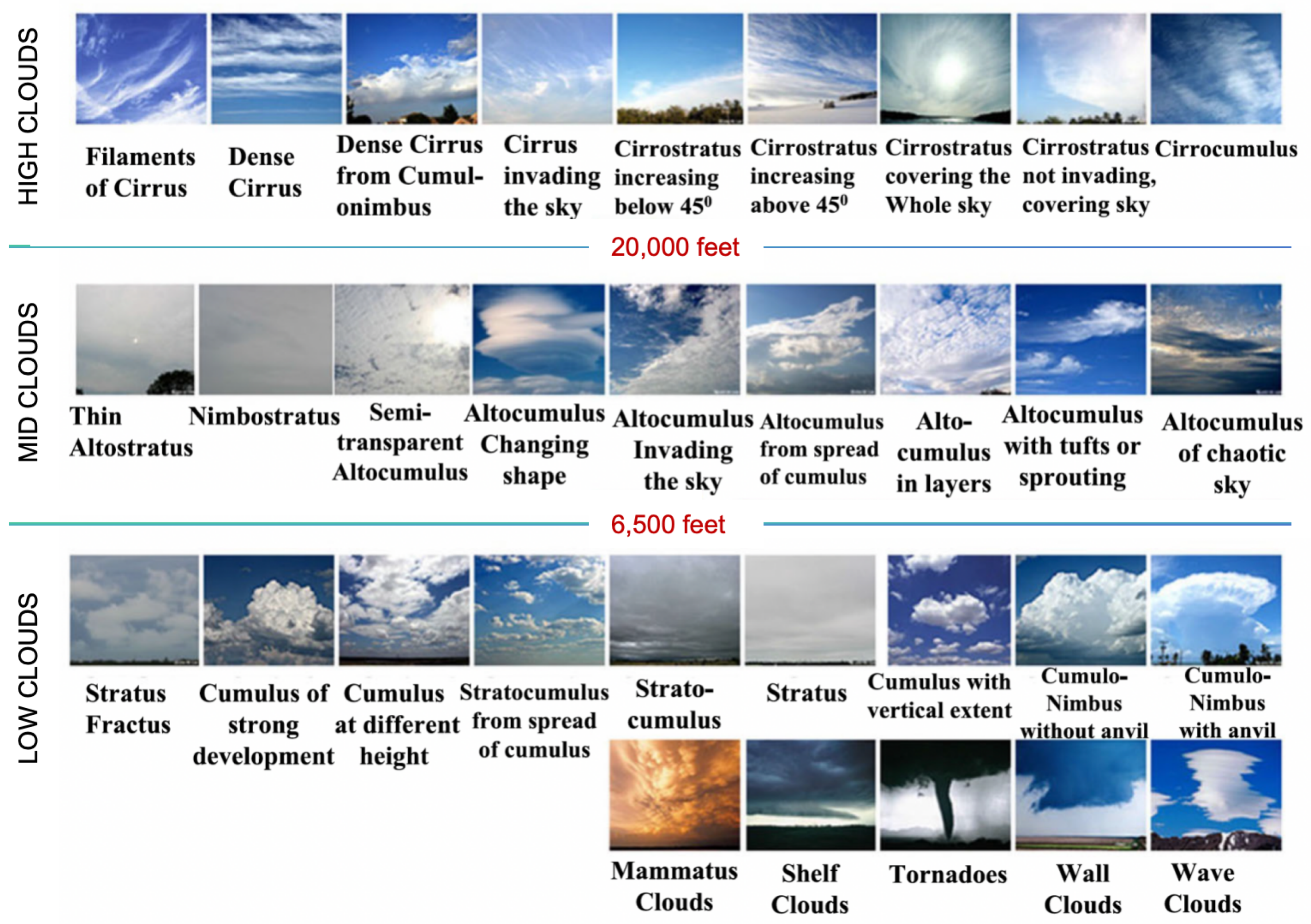
Figure 2.
The pipeline of our proposed CurriCloud. The gray regions represent the full-sample initialization phase and full-sample fine-tuning phase , while the blue region denotes the dynamic curriculum scheduling.
Figure 2.
The pipeline of our proposed CurriCloud. The gray regions represent the full-sample initialization phase and full-sample fine-tuning phase , while the blue region denotes the dynamic curriculum scheduling.
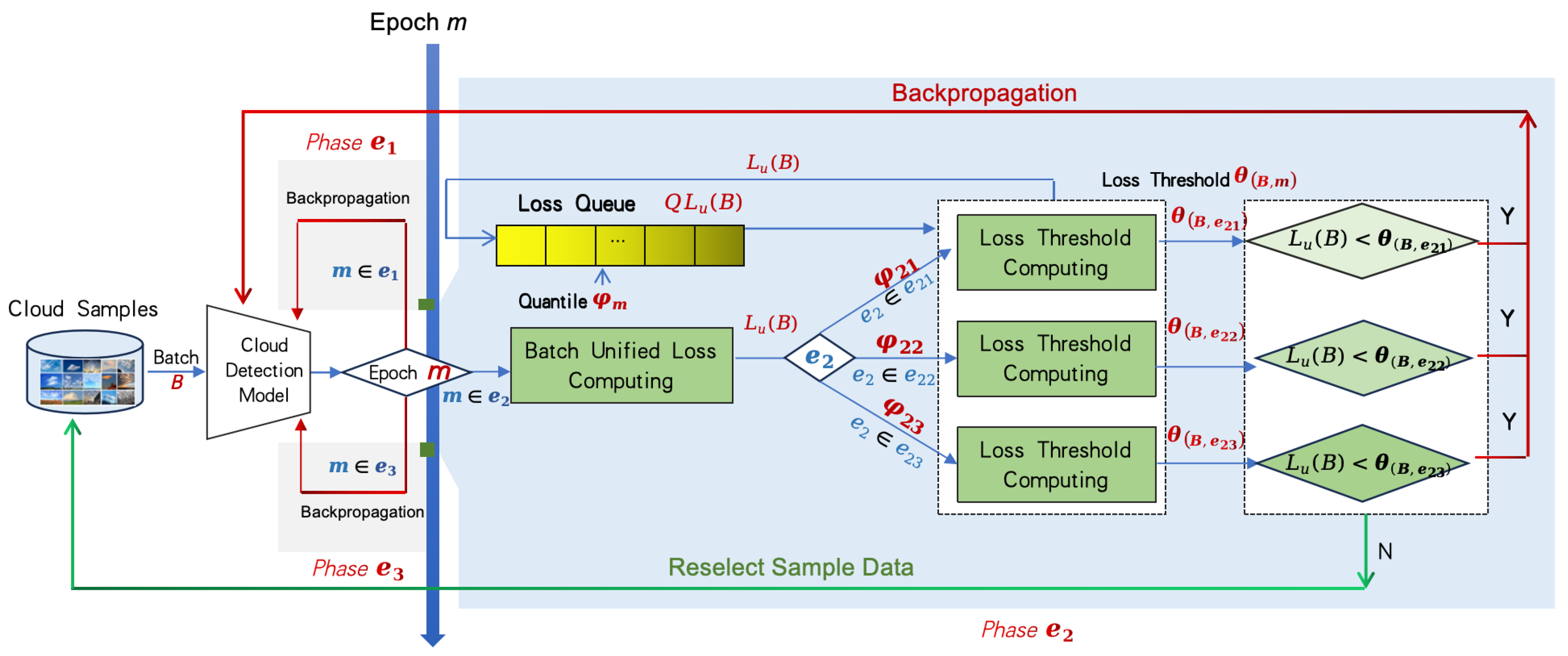
Figure 3.
The loss sliding window queue.
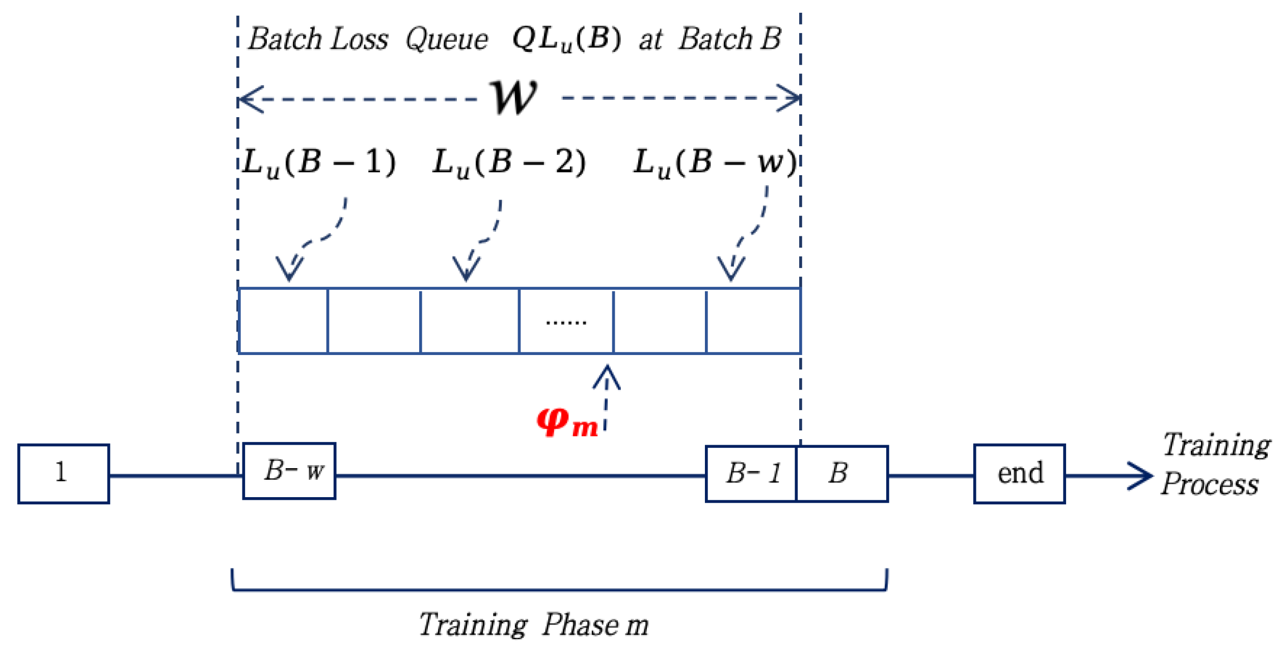
Figure 4.
Some representative cloud types in ALPACLOUD.

Figure 5.
Examples of CurriCloud annotations and results (dark colors represent ground truth boxes, light colors represent predicted boxes, and the same color scheme indicates the same category).
Figure 5.
Examples of CurriCloud annotations and results (dark colors represent ground truth boxes, light colors represent predicted boxes, and the same color scheme indicates the same category).
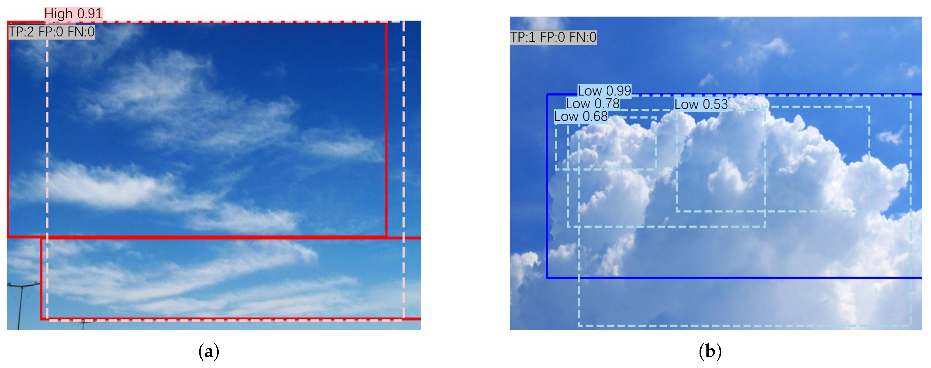
Figure 6.
Visualization of test results on ALPACLOUD.
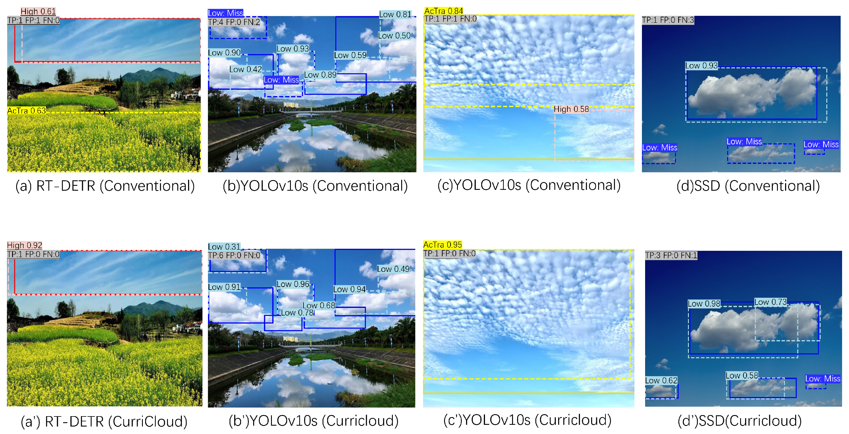
Figure 7.
Loss-epoch curves and precision-recall (P-R) performance respectively for the three strategies on YOLOv10s and RT-DETR-R50 architectures.
Figure 7.
Loss-epoch curves and precision-recall (P-R) performance respectively for the three strategies on YOLOv10s and RT-DETR-R50 architectures.
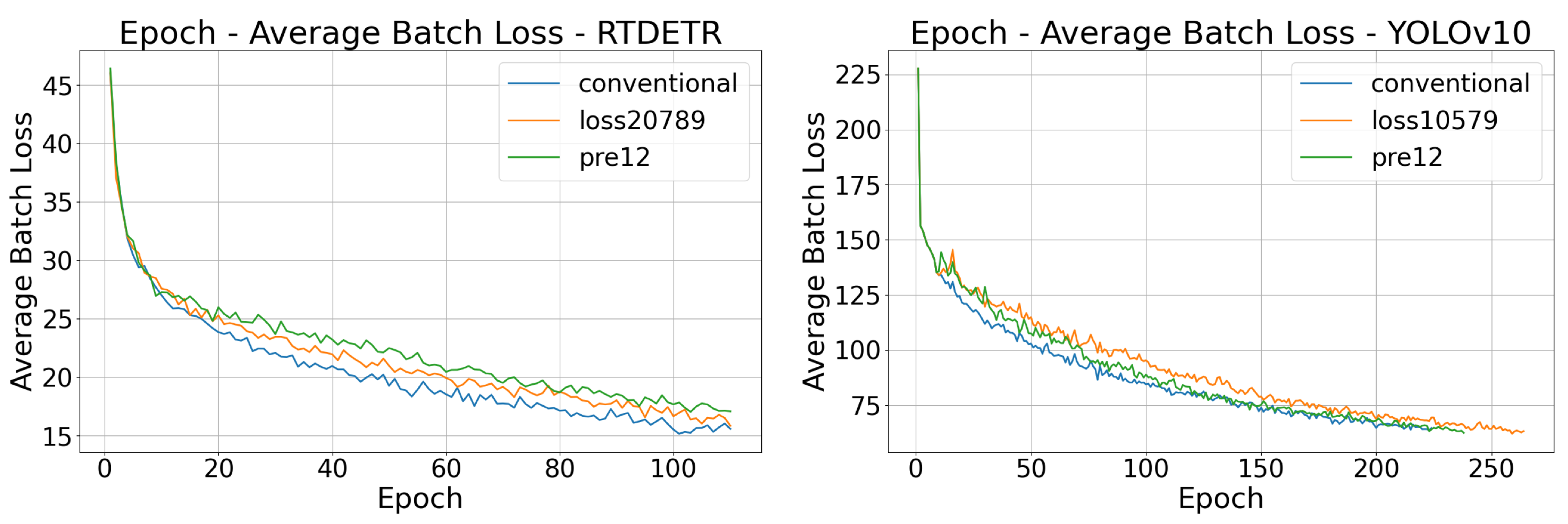
Figure 8.
(P-R) performance for the three strategies on YOLOv10s and RT-DETR-R50 architectures, respectively.
Figure 8.
(P-R) performance for the three strategies on YOLOv10s and RT-DETR-R50 architectures, respectively.
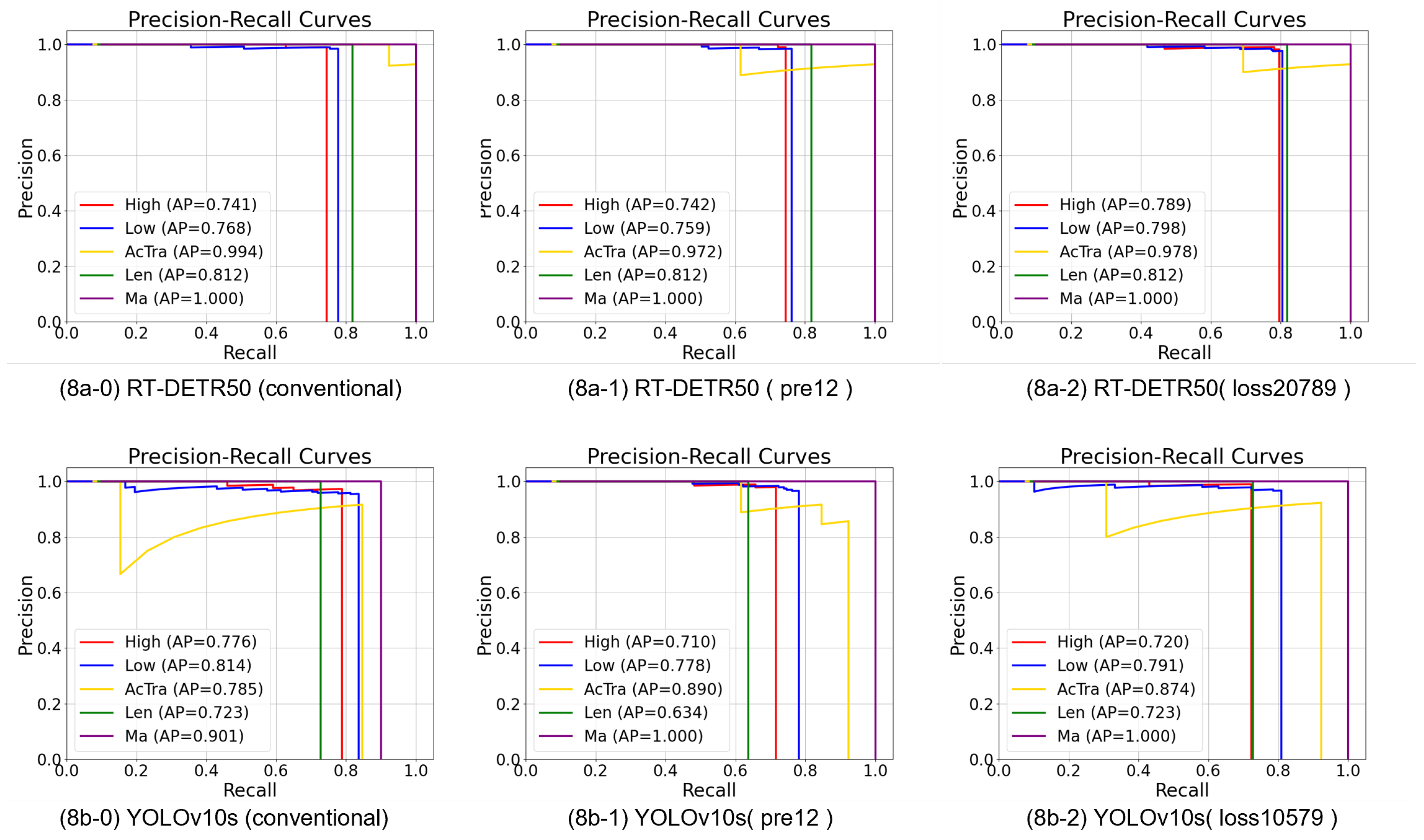

Table 1.
Class descriptions of cloud types in ALPACLOUD
| Index | Class Name | WMO Name | Base Height | Proportion |
|---|---|---|---|---|
| 0 | High | Cirrus(Ci), Cirrocumulus (Cc), Cirrostratus (Cs); |
>20k ft | 37.07% |
| 1 | Low | Cumulus (Cu), Stratocumulus (Sc), Stratus (St); |
<6.5k ft | 46.14% |
| 2 | AcTra | Altocumulus translucidus (AcTra); | 6.5k - 20k ft | 5.94% |
| 3 | Len | Altocumulus lenticularis (AcLen); | 6.5k - 20k ft | 5.38% |
| 4 | Ma | Mammatus clouds (part of Cumulonimbus (Cb)). |
<6.5k ft | 5.49% |
Table 2.
CurriCloud Settings for Different Detectors.
| Detector Model | Training Phase (m) | Epochs | w | |
|---|---|---|---|---|
| YOLOv10s | 1–9 | ∞ | 10 | |
| : 10–49 | 0.5 | |||
| : 50–99 | 0.7 | |||
| : 100–149 | 0.9 | |||
| 150– | ∞ | |||
| RT-DETR-R50 | 1–9 | ∞ | 20 | |
| : 10–29 | 0.7 | |||
| : 30–49 | 0.8 | |||
| : 50–99 | 0.9 | |||
| 100– | ∞ | |||
| ULFG-FD | 1–9 | ∞ | 20 | |
| : 10–29 | 0.7 | |||
| : 30–49 | 0.8 | |||
| : 50–99 | 0.9 | |||
| 100– | ∞ |
Table 3.
Performance comparison between conventional training and CurriCloud on ALPACLOUD dataset (mAP50, Precision, and Recall reported in decimal format).
Table 3.
Performance comparison between conventional training and CurriCloud on ALPACLOUD dataset (mAP50, Precision, and Recall reported in decimal format).
| Model Category | Model | Training Regime | mAP50 | Precision | Recall |
|---|---|---|---|---|---|
| CNN Based | YOLOv10s | Conventional | 0.800 | 0.943 | 0.820 |
| CurriCloud(Ours) | 0.821 | 0.955 | 0.787 | ||
| ULFG-FD | Conventional | 0.442 | 0.878 | 0.557 | |
| CurriCloud(Ours) | 0.556 | 0.835 | 0.593 | ||
| Transformer Based | RT-DETR-R50 | Conventional | 0.863 | 0.977 | 0.780 |
| CurriCloud(Ours) | 0.875 | 0.975 | 0.813 |
Table 4.
Parameter ablation study of CurriCloud with varying queue lengths (w) and threshold quantiles , , and on ALPACLOUD. Bold indicates exceeding the model baseline, and red represents the best performance of the parameter in this model.
Table 4.
Parameter ablation study of CurriCloud with varying queue lengths (w) and threshold quantiles , , and on ALPACLOUD. Bold indicates exceeding the model baseline, and red represents the best performance of the parameter in this model.
| Model | CurriCloud (Ours) | w | mAP50 | Precision | Recall | |||
|---|---|---|---|---|---|---|---|---|
| Yolov10s | Conventional | — | — | — | — | 0.800 | 0.943 | 0.820 |
| loss10579 | 10 | 0.5 | 0.7 | 0.9 | 0.821 | 0.955 | 0.787 | |
| loss10789 | 10 | 0.7 | 0.8 | 0.9 | 0.820 | 0.963 | 0.724 | |
| loss20579 | 20 | 0.5 | 0.7 | 0.9 | 0.831 | 0.939 | 0.756 | |
| loss20789 | 20 | 0.7 | 0.8 | 0.9 | 0.810 | 0.942 | 0.799 | |
| loss40579 | 40 | 0.5 | 0.7 | 0.9 | 0.813 | 0.964 | 0.745 | |
| loss40789 | 40 | 0.5 | 0.7 | 0.9 | 0.772 | 0.910 | 0.801 | |
| ULFG-FD | Conventional | — | — | — | — | 0.442 | 0.878 | 0.557 |
| loss10579 | 10 | 0.5 | 0.7 | 0.9 | 0.554 | 0.845 | 0.550 | |
| loss10789 | 10 | 0.7 | 0.8 | 0.9 | 0.500 | 0.836 | 0.621 | |
| loss20579 | 20 | 0.5 | 0.7 | 0.9 | 0.519 | 0.860 | 0.621 | |
| loss20789 | 20 | 0.7 | 0.8 | 0.9 | 0.556 | 0.835 | 0.593 | |
| loss40579 | 40 | 0.5 | 0.7 | 0.9 | 0.488 | 0.811 | 0.593 | |
| loss40789 | 40 | 0.7 | 0.8 | 0.9 | 0.496 | 0.823 | 0.609 | |
| RT-DETR-R50 | Conventional | — | — | — | — | 0.863 | 0.977 | 0.780 |
| loss10579 | 10 | 0.5 | 0.7 | 0.9 | 0.865 | 0.966 | 0.810 | |
| loss10789 | 10 | 0.7 | 0.8 | 0.9 | 0.851 | 0.971 | 0.789 | |
| loss20579 | 20 | 0.5 | 0.7 | 0.9 | 0.857 | 0.977 | 0.794 | |
| loss20789 | 20 | 0.7 | 0.8 | 0.9 | 0.875 | 0.975 | 0.813 | |
| loss40579 | 40 | 0.5 | 0.7 | 0.9 | 0.839 | 0.968 | 0.773 | |
| loss40789 | 40 | 0.5 | 0.7 | 0.9 | 0.824 | 0.984 | 0.705 | |
Table 5.
Performance comparison with identical hyperparameters across all methods.
| Model | Training Regime | mAP50 | Precision | Recall |
|---|---|---|---|---|
| YOLOv10s | Conventional (Baseline) | 0.800 | 0.943 | 0.820 |
| loss10579(CurriCloud) | 0.821 | 0.955 | 0.787 | |
| pre12-579 (Static CL) | 0.802 | 0.953 | 0.766 | |
| RT-DETR-R50 | Conventional (Baseline) | 0.863 | 0.977 | 0.780 |
| loss20789CurriCloud | 0.875 | 0.975 | 0.813 | |
| pre12-579 (Static CL) | 0.857 | 0.985 | 0.770 |
Disclaimer/Publisher’s Note: The statements, opinions and data contained in all publications are solely those of the individual author(s) and contributor(s) and not of MDPI and/or the editor(s). MDPI and/or the editor(s) disclaim responsibility for any injury to people or property resulting from any ideas, methods, instructions or products referred to in the content. |
© 2025 by the authors. Licensee MDPI, Basel, Switzerland. This article is an open access article distributed under the terms and conditions of the Creative Commons Attribution (CC BY) license (http://creativecommons.org/licenses/by/4.0/).
Copyright: This open access article is published under a Creative Commons CC BY 4.0 license, which permit the free download, distribution, and reuse, provided that the author and preprint are cited in any reuse.


