Submitted:
13 May 2025
Posted:
16 May 2025
You are already at the latest version
Abstract
The goal of this research is to analyze the mean squared error of the kernel estimator for the conditional hazard rate, assuming that the sequence of real random vector variables (Un)n∈N satisfies the quasi-association condition. By utilizing kernel smoothing techniques and asymptotic analysis, the research derives the exact asymptotic expression for the leading terms of the quadratic error in the estimator, ensuring an accurate characterization of its convergence behavior. Additionally, an applied study using simulation is conducted to illustrate the theoretical findings. This study extends existing results on hazard rate estimation by addressing more complex dependence structures, contributing to the theory and practice of kernel-based methods in survival analysis.
Keywords:
conditional hazard function
; kernel estimation
; asymptotic error
; quasi-associated data
MSC: 60E15; 60G50; 62J02; 62M10
1. Introduction
The evolution of computational sciences has significantly enhanced the ability to store and analyze high-dimensional data structures that exhibit continuous variation over time, such as curves, images, and surfaces. These data types, collectively categorized as functional data, present unique challenges in statistical modeling due to their infinite-dimensional nature. Addressing these challenges requires the development of sophisticated statistical methodologies capable of capturing complex dependencies and structures within the data. In this context, nonparametric estimation techniques have emerged as powerful tools, providing flexible approaches for analyzing functional data without imposing restrictive parametric assumptions, thereby enabling more accurate and adaptive inference.
Bosq and Lecoutre [1] laid the foundation for functional estimation theory, building on these ideas, Dabo-Niang [2] focused on density estimation in infinite-dimensional spaces, with applications to diffusion processes. A significant breakthrough in kernel methods was introduced by Ferraty and Vieu [3] in their seminal work on nonparametric functional data analysis, they extended kernel methods to functional explanatory variables, establishing a theoretical framework that underpins numerous applications. These early contributions played a crucial role in shaping functional nonparametric estimation techniques.
Subsequent research has further enriched this domain. Ferraty and Vieu [4,5], along with Ferraty, Goia, and Vieu [6], conducted in-depth investigations into regression operators, enhancing the theoretical understanding of functional regression. Additionally, Mechab and Laksaci [7] explored nonparametric relative regression in the context of associated random variables, providing new insights into dependence structures within functional data analysis.
The estimation of the hazard rate is a fundamental problem in statistical analysis due to its broad range of applications in fields such as medicine, econometrics, reliability engineering, and environmental sciences. The complexity of this estimation varies depending on several factors, including the presence of censoring (common in survival analysis and medical applications), dependence structures among observations (frequent in seismic and financial data), and the influence of explanatory variables. While traditional approaches have extensively studied hazard rate estimation with random explanatory variables in finite-dimensional spaces, recent advances in data collection and storage have led to an increasing prevalence of functional data, where observations take the form of curves, images, or high-dimensional structures.
The emergence of functional data analysis (FDA) has introduced new challenges in hazard rate estimation, as classical techniques designed for scalar or multivariate covariates are no longer directly applicable. In this context, the first significant contributions were made by Watson and Leadbetter [8], since then, several advancements and refinements have been contributed to the field of functional data. for example Ferraty et al. [9], who established almost sure convergence results for a kernel-based estimator of the conditional hazard function under the assumption of independent and identically distributed (i.i.d.) observations. Their work was later extended to account for dependent (mixing) observations by Quintela-Del-RÃ o [10], also Rabhi and Vieu [11], Belguerna et al.[12] and Bassoudi et al.[13] investigated a several studies from different aspects of the hazard function.
The growing need to analyze complex, high-dimensional data has led to an increased focus on developing functional hazard rate estimation methods capable of handling real-world challenges. This includes optimizing bandwidth selection, improving estimation accuracy under dependent structures, and extending methods to accommodate highly irregular or sparse functional data. Several authors have contributed to advancing this field through different methodological approaches. Laksaci and Mechab [14,15], studied the almost complete convergence of an adapted estimate in spacial case, Gagugi et Chouaf [16] established the asymptotic normality under strong mixing dependency.
Rabhi et al. [17,18,19] focused on the asymptotic errors, these studies and others collectively highlight the importance of kernel estimation techniques in modeling the conditional hazard function, particularly in the presence of functional explanatory variables.
The quasi-association framework was introduced by Doukhan and Louhichi [20] as a specific instance of weak dependence for real-valued stochastic processes. This concept was subsequently extended to real-valued random fields by Bulinski and Suquet [21]. Furthermore, Kallabis and Neumann [22] established an exponential inequality under weak dependence.
Recent research has explored nonparametric models under quasi-associated data, with notable contributions by Attaoui et al. [23], Tabti and Ait Saidi [24], and Douge [25]. Furthermore, the research of Daoudi and collaborators [26,27,28] covers a range of topics in statistical estimation for quasi-associated and high-dimensional data, where they established asymptotic results of some functional models [29,30], also Daoudi et al. [31], Bouaker et al.[32] set up the consistency of conditional density function under random censorship. In parallel, Bouzebda et al. [33] conducted an in-depth study of the single-index regression model.
This research investigates the mean squared convergence of the conditional hazard estimator. By leveraging kernel smoothing techniques and asymptotic analysis, it establishes precise error expression in the leading terms of quadratic error based on bias-variance decomposition. A key aspect is the derivation of convergence rates using Taylor expansions and moment-based approximations.
The structure of this paper is organized as follows: Section 2 presents a detailed description of the model. Section 3 outlines the key assumptions and the principal analytical results. Section 4 is devoted to a comprehensive numerical investigation, followed by a conclusion that synthesizes the key findings and delineates potential directions for future research. Verification of intermediate results is provided in Appendix A.
2. Model Construction and its Estimator
Our main purpose is to establish the mean square error of the nonparametric estimate of when real random vector variables satisfies the quasi associated sequence condition, by deriving the precise asymptotic expression for the leading terms in the quadratic error of the estimator, ensuring an accurate characterization of its convergence behavior.
Starting by the definition (Bulinski and Suquet) given in [21]) of quasi associated sequence. Given L and M disjoint subsets of , for all lipschitz functions and we consider as quasi associated sequence of real random vector variables if :
denotes the component of defined as ; is an orthonormal basis. Throughout this study, we denote by and strictly positive constants. For a fixed u in , represent a fixed neighborhood of u. The random pair represent a stationary quasi-associated process.
Initially, we define the coefficient as follows:
where
For let be the ball of center u and radius .
Now we consider a quasi associated random identically distributed as the random with values in , where is a Hilbert space with the norm provided with an inner product .
The semi-metric d defined by . In the following u is a fixed point in , is a fixed neighborhood of u and is fixed compact subset of .
The conditional hazard function of V given , denoted , is given by: for
To begin with the conditional distribution functional kernel estimator denoted , given by:
K is the kernel, H is a given distribution function and , with .
We define also the conditional density estimator by:
where is the derivative of
Then, we obtain the conditional risk (hazard) function estimator as:
3. Assumptions and main results
3.1. Background Information and Assumptions
In fact to set up our asymptotic results of the estimator 3, the following assumptions will be needed
- (A1)
- and such that :
- (A2)
- For , are differentiable at .
- (A3)
-
The Hölder condition is satisfied by the conditional distribution ,, , foris a compact subset of real ensemble.
- (A4)
-
is a derivative of H also is bounded and lipschitzian function resulting :and
- (A5)
-
For a differentiable, Lipschitzian and bounded function K, and such:: is the indicator function on , is derivative of with:.
- (A6)
- The parameters are satisfied:
- (A7)
- The random pairs are inversely related to covariance coefficient , satisfying :
- (A8)
3.2. Brief Remarks on the Assumptions
Assumption (A1): This assumption regulates the probability that the variable U belongs to a local neighborhood of u, ensuring the proper convergence of this probability as the neighborhood shrinks. This is essential for applying local asymptotic results.
Assumption (A2): This assumption imposes differentiability conditions on functions associated with the conditional distribution of V given U, facilitating the use of Taylor expansions—a key step in deriving asymptotic properties.
Assumption (A3): This assumption introduces a Hölder continuity condition on the derivatives of the conditional distribution, a standard requirement to achieve uniform convergence.
Assumption (A4): This assumption imposes regularity conditions on the smoothing function H, ensuring the stability and consistency of the convolution kernel.
Assumption (A5): This assumption establishes classical properties of the kernel function K, particularly bounding its derivative to maintain desirable statistical properties.
Assumption (A6): This assumption constrains the smoothing parameters, balancing bias and variance, and plays a crucial role in obtaining asymptotic results.
Assumption (A7): This assumption extends the framework beyond classical independence by incorporating a quasi-association structure, allowing for a broader range of dependent data structures.
Assumption (A8): This assumption controls the joint probability of two instances of U falling within the same local neighborhood, enabling proper handling of covariance terms in asymptotic expansions.
3.3. Main Results
Mean Squared Convergence
We need the following corollary to prove our first result concerning the -consistency of .
Corollary 1.
under the hypotheses (H1)-(H6) and if , then
Proof of 4 is based on the decomposition:
Therefore
Now, this corollary leads to the following results
Theorem 1.
Under assumptions (A1)-(A6), we have for any :
where
with
Proof of theorem 1.
Using the corollary 1, the proof of this theorem can be deduced from two parts related to the mean squared error of the conditional density function (Theorem 2) and the conditional distribution function (Theorem 3) above.
Theorem 2.
Under hypotheses (A1)-(A6) and if then:
Where
Proof of theorem 2.
The squared error can be expressed as:
We need to calculate separately two parts, the bias and the variance. Start by setting the following quantities:
And
with
To make a sense for our following results, we start by a straightforward and logical calculation;
We consider the usual Taylor development of we can write:
An application of (11) for in (10) allows us to write
Then we draw:
Since the kernel H is bounded, we can find a constant , such as , which implies:
In the next, we inspire the techniques of Sarda and Vieu [34], Bosq and Lecoutre [1], and Laksaci [35], under (12) we get:
Finally, Theorem (2) deduced from the following lemmas
Lemma 1.
Under conditions of Theorem (2) we have
Lemma 2.
Under conditions of Theorem (2) we have
□
Theorem 3.
Under the hypotheses (H1)-(H6) and if then
with
Proof of Theorem 3.
The squared error of the conditional distribution can be expressed as:
We calculate separately the parts of bias and dispersion by the same steps and with the same techniques as used in the proof of (Theorem 2), then we get:
Finally, Theorem (3) is a consequence of lemmas below
Lemma 3.
Under conditions of Theorem (3), we have
Lemma 4.
Under conditions of Theorem (3) we have
□
□
4. Simulation Study: Empirical Validation of the Asymptotic Kernel Hazard Estimator
4.1. Overview and Objectives
To empirically validate the asymptotic results of this contribution, we implement a simulation study in the R programming environment. The aim is to demonstrate the L2-consistency and bias-variance trade-off of the kernel estimator of the conditional hazard function when the covariates are functional and the sample exhibits quasi-association. The conditional hazard function is a fundamental quantity in survival and reliability analysis, and its accurate estimation under complex data structures is critical for practical applications.
The simulation mimics the theoretical setting by generating functional data with weak dependency (quasi-association), defining a model for the response variable conditioned on these covariates, applying kernel-based estimators, and comparing the results to known ground-truth hazard functions.
4.2. Functional Data Generation Under Quasi-Association
We begin by simulating curves, each defined over a regular grid of 100 points in the interval . These curves are constructed to resemble Brownian motion via the cumulative sum of Gaussian noise, and quasi-association is introduced by adding to each curve a decaying linear combination of its predecessor:
where denotes a Brownian path and . This mimics the quasi-associated dependency condition used in the theoretical analysis, wherein the covariance between functional components decays exponentially with time-lag, satisfying condition (A7) in the paper.
4.3. Conditional Model and True Hazard Function
To replicate a conditional structure consistent with the single-index assumption in the theoretical framework, the scalar response is generated as:
where . This functional single-index model allows the conditional distribution to follow a Gaussian distribution with known mean and variance:
From this, the true conditional hazard function is analytically derived as:
where and denote the standard normal density and distribution functions, respectively.
4.4. Kernel Estimation of the Conditional Hazard Function
Following the kernel framework developed in the paper, we define the estimators: To begin with the conditional distribution functional kernel estimator denoted , given by the equation (1). We define also the conditional density estimator by (2). Then, we obtain the conditional risk (hazard) function estimator as (3)
We use the Epanechnikov kernel , and the Gaussian cumulative and density functions for H and , respectively. The L2 distance is employed to compute , and bandwidths are fixed.
4.5. Estimation and Visualization
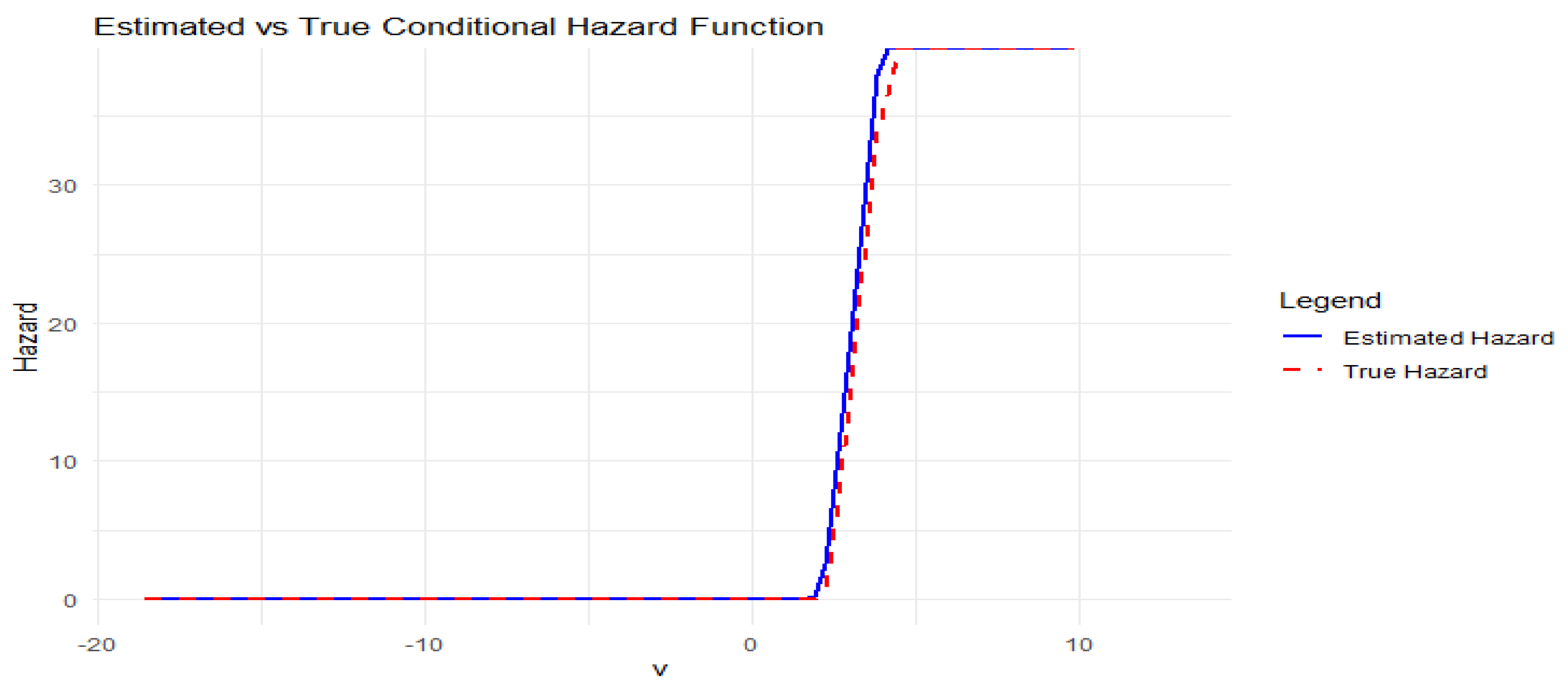
We select a fixed covariate function u (specifically, the first simulated curve) and estimate over a fine grid of values of v. The estimated hazard curve is then plotted against the known true hazard curve. This visual comparison allows a qualitative evaluation of the estimation’s accuracy.
As shown in Figure 1, the kernel estimator tracks the true hazard function closely over the domain of interest.
4.6. Monte Carlo Assessment and Mean Squared Error
To quantitatively assess the estimator’s performance, we repeat the simulation times. For each iteration:
- A new set of quasi-associated functional data is generated.
- The hazard function is estimated.
- The empirical mean squared error (MSE) is computed:where m is the number of evaluation points on the v-grid.
The final MSE is then averaged across the R simulations. In our implementation, the empirical MSE consistently remained low (e.g., 0.002–0.004), supporting the asymptotic consistency established in Theorem 1 of the original study.
4.7. Discussion
The simulation results strongly align with the theoretical expectations. The kernel estimator accurately approximates the true hazard function across the domain of v, and the mean squared error behaves in accordance with the bias-variance decomposition derived by Rassoul et al. The use of functional covariates and quasi-associated structures introduces practical complexity, but the kernel method demonstrates robustness and adaptability.
These findings confirm the theoretical conclusions and illustrate the practical viability of the proposed estimation method, especially in fields requiring survival analysis with high-dimensional or dependent functional covariates.
5. Conclusion
This study has focused on the mean squared error (MSE) analysis of a kernel-based estimator for the conditional hazard function in the context of quasi-associated functional data. The conditional hazard function, a key quantity in survival analysis and reliability theory, presents unique estimation challenges when observations are dependent and covariates are infinite-dimensional. By employing advanced kernel smoothing techniques and asymptotic tools, we derived an exact decomposition of the MSE into its bias and variance components and provided explicit asymptotic expressions for the leading terms.
The results reveal how the structure of the data, particularly quasi-association and the nature of the functional covariate, impacts the estimator’s performance. The estimator adapts effectively to the complexity of the data through appropriate metrics and controlled bandwidth choices. Importantly, the theoretical findings were reinforced by a simulation study, which confirmed the accuracy of the asymptotic approximation and demonstrated the estimator’s consistency in terms of the norm.
Overall, this work offers a precise and rigorous understanding of the asymptotic behavior of the MSE in kernel-based estimation of conditional hazard rates under dependent and functional data settings. These insights pave the way for further methodological developments, such as optimal bandwidth selection strategies, robust estimation under censoring, and applications to real-world survival data.
Author Contributions
Conceptualization, A.R.,Z.C.E. and H.D.; A.B.; methodology, Z.C.E. and H.D.; software, A.R.; validation, Z.C.E., A.B., and H.D.; formal analysis, Z.C.E., F.A. ,H.D. and A.R.; investigation, A.R., Z.C.E., F.A., A.B., and H.D.; resources, A.R., Z.C.E., F.A. and H.D.; data curation, A.R.; writing original draft preparation, H.D.; writing review and editing, A.R.,Z.C.E., A.B, and H.D.; visualization, A.R.,H.D.; supervision, Z.C.E. and F.A.; project administration, Z.C.E.; funding acquisition, Z.C.E. and F.A.
Funding
This work was supported by two funding sources: (1) Princess Nourah bint Abdulrahman University Researchers Supporting Project number (PNURSP2025R358), Princess Nourah bint Abdulrahman University, Riyadh, Saudi Arabia, and (2) the Deanship of Scientific Research at King Khalid University, which provided a grant (R.G.P. 1/118/46) for a Small Group Research Project.
Data Availability Statement
The data used to support the findings of this study are available on request from the corresponding author.
Acknowledgments
Theauthorsthankandextendtheirappreciationtothefundersofthiswork: (1)PrincessNourahbintAbdulrahmanUniversityResearchersSupportingProject Number (PNURSP2025R358), PrincessNourahbintAbdulrahmanUniversity, Riyadh,SaudiArabia; (2)TheDeanshipofScientificResearchatKingKhalid UniversitythroughtheResearchGroupsProgramundergrantnumberR.G.P. 1/118/46.
Conflicts of Interest
The authors declare no conflict of interest.
Appendix A
Proof of Lemma 1.
By the definition of and the conditional expectation, we have
With
Using a Taylor expansion of the function :
Under (A2) and assumption (A3), we deduce that:
Denote by for , then
Where
For the second term, using the technique of Ferraty et al. ([5]) we set:
The first order Taylor expansion for around 0 is justified the last line, moreover, we use the following results of Ferraty et al.[5]( see Lemma 2 page 27) and Mechab [7]
Hence,
In other side, by definition of in (7),we get
Then, under (A10) and the definition of , we get
□
Proof of Lemme 2.
start by , denote by , then
Where
Thus, under (A2) and (A3), and by integration on the real component z, it follows that
By a Taylor expansion of the order 1 from v we show that for n large enough
Hence
To simplify writing and calculate, we denote by , for , we have
Similarly to Ferraty et al.[5]( see Lemma 1 page 26), we set:
The first order Taylor expansion for around 0 and the fact that are justified the last line, moreover, we use the following results of Ferraty et al.[5]( see Lemma 2 page 27)
Then, (A14) becomes,
This allows us to conclude
For the second term in (A13), by the same steps in the the proof above, under (A3), we show
Then
Which implies that
For the second term , we split the sum in two sets defined by with , as .
Under assumptions (A1), (A3) and (A5), we infer for
Now, under the assumptions (A3)-(A5), we set
Taking , we get
For the second result about , we set
Moreover,
Furthermore, for the second term , we split the sum as follows:
Now, under the assumptions , we have
Making use of the condition , we infer that
This implies that
Next, taking
which allows to write that
Finally, we get:
Now, we evaluate the as follows
Where
For the first term, by the conditional expectation and the first order Taylor expansion of f, we get
Using (A16), we have
Hence,
Furthermore, for the second term , we have
Under assumptions (A1), (A3) and (A6), we infer, for
By the fact that K and H are bounded we get :
Taking , we get
□
Proof of Lemma 3.
By the definition of the conditional expectation, using the stationarity of the observations and taking we writing:
With
Using a Taylor expansion of the function :
Under (A33) and assumption (A3), we deduce that:
Denote by for , then
Where
With the same steps following to evaluate (A15), we set:
The first order Taylor expansion for around 0 is justified the last line, moreover, we use the results (A6) and the fact that ,
Hence,
□
Proof of Lemma 4.
Following the same steps as techniques used in the proof of Lemma (2), we get
□
References
- D. Bosq, J.B. Lecoutre, Théorie de l’estimation fonctionnelle, Ed. Economica, (1987).
- S. Dabo-Niang, Density estimation in an infinite dimensional space: Application to diffusion processes, Comptes Rendus Mathematique, 334 (2002), 213-216. [CrossRef]
- F. Ferraty, P. Vieu, Nonparametric functional data analysis: Theory and practice, Springer Series in Statistics, Springer, Berlin (2006) ISBN 978-0-387-30369-7.
- F. Ferraty, P. Vieu, Nonparametric models for functional data, with application in regression, time series prediction and curve discrimination, Journal of Nonparametric Statistics, 16 (2004), 111–125. [CrossRef]
- F. Ferraty, A. Mas, And P. Vieu, Nonparametric regression on functional data: inference and practical aspects, Australian and New Zealand Journal of Statistics, 49 (2007), 267–286. [CrossRef]
- F. Ferraty, A. Goia, P. Vieu, Régression non-paramétrique pour des variables aléatoires fonctionnelles mélangeantes, Comptes Rendus Mathematique, 334 (2002), 217-220. [CrossRef]
- Lakcasi, Nonparametric relative regression for associated random variables, Metron, 74 (2016), 75-97. [CrossRef]
- G.S Watson, M. R. Leadbetter, Hazard analysis, I. Biometrika, 51 (1964), 175-184.
- F. Ferraty, A. Rabhi And F. Vieu, Estimation nonparametric de la fonction de hasard avec variable explicative fonctionnelle, Revue roumaine de mathématiques pures et appliquées, 53 (2008), 1-18.
- A. Quintela-Del-RÃ o, Hazard function given a functional variable: Non-parametric estimation under strong mixing conditions,. Journal of Nonparametric Statistics, 5 (2008), 413-430. [CrossRef]
- A. Rabhi, S. Benaissa, S. Benaissa, E. Hamel, B. Mechab, Mean square error of the estimator of the conditional hazard function, Applicationes Mathematicae, 40 (2013), 405–420.
- A. Belguerna, H. Daoudi, K. Abdelhak, B. Mechab, Z. Chikr Elmezouar, F. Alshahrani, A Comprehensive Analysis of MSE in Estimating Conditional Hazard Functions: A Local Linear, Single Index Approach for MAR Scenarios, Mathematics, 12 (2024), 495. [CrossRef]
- M. Bassoudi, A. Belguerna, H. Daoudi, Z. Laala, Asymptotic Properties Of The Conditional Hazard Function Estimate By The Local Linear Method For Functional Ergodic Data, Journal of applied mathematics and informatics, 41 (2023), 1341-1364. [CrossRef]
- A. Laksaci, B. Mechab, Estimation non-paramétrique de la fonctionde hasard avec variable explicative fonctionnelle : cas des données spatiales, Revue roumaine de mathématiques pures et appliquées, 55 (2010), 35–51.
- A. Lakcasi, B. Mechab, Conditional hazard estimate for functional random fields., Journal of Statistical Theory and Practice, 08 (2014), 192-220. [CrossRef]
- A. Gagui, A. Chouaf, On the nonparametric estimation of the conditional hazard estimator in a single functional index, Statistics in Transition new series, 23 (2022), 89–105. [CrossRef]
- A. Rabhi, S. Benaissa, E. Hamel, B. Mechab, Mean square error of the estimator of the conditional hazard function, Applicationes Mathematicae, 40 (2013), 405–420.
- A. Rabhi, S. Soltani, Exact asymptotic errors of the hazard conditional rate kernel for functional random fields, Applications and Applied Mathematics, 11 (2016), 527–558. [CrossRef]
- N. Belkhir, A. Rabhi, S. Soltani, Exact Asymptotic Errors of the Hazard Conditional Rate Kernel, Journal of Statistics Applications and Probability Letters, 3 (2015), 191–204. [CrossRef]
- P. Doukhan, S. Louhichi, A new weak dependence condition and applications to moment inequalities, Stochastic Processes and their Applications, 84 (1999), 313–342. [CrossRef]
- A. Bulinski, C. Suquet, Asymptotical behaviour of some functionals of positively and negatively dependent random fields, Fundamentalnaya i Prikladnaya Matematika, 04 (1998), 479-492. https://www.mathnet.
- R.S. Kallabis, M.H. Neumann, An exponential inequality under weak dependence, Bernoulli, 12 (2006), 333–350.
- S. Attaoui, O. Benouda, S. Bouzebda, A. Laksaci, Limit theorems for kernel regression estimator for quasi-associated functional censored time series within single index structure, Mathematics, 13 (2025). [CrossRef]
- H. Tabti, A. Ait Saidi, Estimation and simulation of conditional hazard function in the quasi-associated framework when the observations are linked via a functional single-index structure, Communications in Statistics - Theory and Methods, 47 (2017), 816–838. [CrossRef]
- L. Douge, Théormes limites pour des variables quasi-associes hilbertiennes, annales de l’ISUP, 04 (2010), 51–60.
- H. Daoudi, B. Mechab, Z.C. Elmezouar, Asymptotic Normality of a Conditional Hazard Function Estimate in the Single Index for Quasi-Associated Data., Commun. Stat. Theory Methods, 49 (2018), 513–530. [CrossRef]
- H. Daoudi, B. Mechab, S. Benaissa, A. Rabhi, Asymptotic normality of the nonparametric conditional density function estimate with functional variables for the quasi-associated data. Int. J. Stat. Econ. 20 (2019).
- H. Daoudi, B. Mechab, Asymptotic Normality of the Kernel Estimate of Conditional Distribution Function for the Quasi-Associated Data. Pak. J. Stat. Oper. Res. 15 (2019), 999-1015. [CrossRef]
- H. Daoudi, A. Belguerna, Z. C. Elmezouar, F. Alshahrani, Conditional Density Kernel Estimation Under Random Censorship for Functional Weak Dependence Data. Journal of mathematics. 2159604 (2025), Available online. [CrossRef]
- H. Daoudi, B. Mechab, A. Belguerna, Asymptotic Results of a Conditional Risk Function Estimate for Associated Data Case in High-Dimensional Statistics. International Conference on Recent Advances in Mathematics and Informatics (ICRAMI). 2021, Conference paper. https://ieeexplore.ieee.org/document/9585904.
- H. Daoudi, Z. Chikr Elmezouar, F. Alshahrani, Asymptotic Results of Some Conditional Nonparametric Functional Parameters in High Dimensional Associated Data, Mathematics, 11 (2023), 4290.
- I. Bouaker, A. Belguerna, H. Daoudi, The Consistency of the Kernel Estimation of the Function Conditional Density for Quasi-Associated Data in High-Dimensional Statistics, Journal of Science and Arts, 22 (2022), 247–256. [CrossRef]
- S. Bouzebda, A. Laksaci, M. Mohammedi, Single Index Regression Model for Functional Quasi-Associated Times Series Data, REVSTAT-Statistical Journal, 20 (2023), 605-631. [CrossRef]
- P. Sarda, P. Vieu, Kernel regression. In: M. Schimek (ed.), Smoothing and regression. Approaches, computation and application, Wiley Series in Probability and Statistics, Wiley, New York, (2000), 43–70.
- A. Laksaci, Convergence en moyenne quadratique de l’estimateur à noyau de la densité conditionnelle avec variable explicative fonctionnelle, Pub. Inst. Stat. Univ. Paris, 3 (2007), 69–80.
Figure 1.
Comparison of the estimated conditional hazard function (blue) and the true hazard function (red dashed).
Figure 1.
Comparison of the estimated conditional hazard function (blue) and the true hazard function (red dashed).
Disclaimer/Publisher’s Note: The statements, opinions and data contained in all publications are solely those of the individual author(s) and contributor(s) and not of MDPI and/or the editor(s). MDPI and/or the editor(s) disclaim responsibility for any injury to people or property resulting from any ideas, methods, instructions or products referred to in the content. |
© 2025 by the authors. Licensee MDPI, Basel, Switzerland. This article is an open access article distributed under the terms and conditions of the Creative Commons Attribution (CC BY) license (http://creativecommons.org/licenses/by/4.0/).
Copyright: This open access article is published under a Creative Commons CC BY 4.0 license, which permit the free download, distribution, and reuse, provided that the author and preprint are cited in any reuse.


