
Submitted:
25 April 2025
Posted:
28 April 2025
You are already at the latest version
Abstract
We present techniques for a machine learning approach to predict stellar classes of stars using their physical and observable characteristics. Stellar classification is the categorization of stars into spectral types and subclasses based on temperature, color, and various other properties, and it is a fundamental aspect of astronomy, providing vital insights into stellar properties and evolutionary stages. By taking the general class of a star (e.g., G2 being the Sun), our model leverages a diverse range of input features, such as luminosity, surface temperature, and color indices, to predict a star’s spectral class with viable accuracy. Among several implemented algorithms, Random Forest Classifier achieved an accuracy of 76% (log loss 0.69), outperforming other methods such as XGBoost (71%), K-Nearest-Neighbors (50%), and Logistic Regression (23%). We attribute the lower performance of XGBoost to overlapping threshold features and K-Nearest-Neighbors to the low linear correlations of the data. The results demonstrate the high potential of machine learning to automate feature classification within astronomy, such as spectral classification efficiently and with high accuracy, significantly enhancing our capacity to analyze large data sets in modern astronomy.
Keywords:
Machine Learning
; Stellar Classification
; Astronomy
; Data Analysis
; Spectral Types
; Prediction
; Stars
1. Introduction
From white dwarfs to red giants, stars have a complex and fascinating life cycle that has been studied extensively in astronomy. With such a large number of these celestial bodies scattered across space, fostering a deeper understanding of their development is crucial in our comprehension of the universe. Even with recent developments and innovations in the field of astronomy, predicting stellar evolution manually, even with strict guidelines, has remained elusive due to many factors, including mass, environment, and composition, that influence a star’s evolution.
In recent years, machine learning has noticeably been a capable alternative, with its capacity to analyze and draw insights from large volumes of data. This study explores the application of machine learning in predicting the life cycle stages of stars by analyzing a data set of photometric measurements (magnitudes in different bands), temperature, luminosity, and spectral classifications. By automating the classification process, our approach alleviates the labor-intensive nature of traditional techniques. The data set used in this study was largely derived from the Sloan Digital Sky Survey (SDSS), augmented with additional observations from ancillary astronomical databases.
Our research aims to not only enhance our understanding of stellar evolution but also to provide a starting point to expand upon for future large-scale astrophysical works, assisting in endeavors for analysis in years to come.
2. Materials and Methods
Our methods combine the usage of multiple tools and techniques to predict the evolutionary stage and corresponding spectral class of a star from its observable characteristics. Our model was created with Python 3.8 in a Jupyter Notebook environment, facilitating real-time data visualization, feature engineering, and iterative model development. In this section, we discuss the steps to which we acquired data, selected features, and trained/evaluated the model.
a. Data Collection
Most of the data was obtained by astronomical surveys, primarily the Sloan Digital Sky Survey (SDSS) [York], supplemented by additional resources like the HYG Database [Unknown Author]. The unfiltered data set contained roughly 100,000 stellar observations covering a comprehensive range of spectral types, evolutionary stages, and stellar parameters such as temperatures, mass estimates, luminosity, and color indices. Prior to analysis, the data underwent extensive filtering in the form of pre-processing, including the filtering of incomplete entries, estimated values, and the normalization of quantitative parameters. Supplementary data from other sheets of the database were integrated to increase the diversity and quality of the sample, ensuring that low-luminosity red dwarfs, active giants, and other stellar outliers were adequately represented.
This data is key to understanding the class balance and important features in the distribution plot. It helps to not only identify if the dataset is imbalanced, which could lead to a biased model that performs poorly for underrepresented classes, but also to identify possible errors in the dataset if there are unexpected spikes or gaps on the graph. This also provides us with a baseline for the expected frequency of each class when using our model to identify stars.
The photometric indices shown in the graph often correlate with stellar properties such as metallicity and temperature, with these patterns helping in guiding feature selection. This diagram also helps with detecting outliers in our data. If points fall outside expected regions, this may indicate issues like bad photometric data. Identifying these flaws allows us to improve the quality of our data, increasing the reliability of our model (Figure 1).
This furthers the results seen in the previous image by adding a third axis- luminosity- to the diagram. While the two-dimensional plot helps distinguish spectral classes based on color alone, this three-dimensional perspective offers a deeper understanding of underlying patterns between brightness and color (Figure 2).
b. Feature Selection and Engineering
Previously, the selection of specific features from our data set was mentioned, and this feature selection used in the study played an extremely important role in determining how well the model could distinguish certain characteristics. This ultimately means that selecting the right features (variables & characteristics) was critical in improving the relative accuracy. In machine learning, feature selection assists in eliminating unneeded or redundant information, which could potentially hinder the model’s performance in prediction. We have calculated primary photometric color indices (e.g., g-r, i-z). These are differences in brightness between specific wavelengths of light observed from stars. For example:
g-r: Difference between the green (g) and red (r) bands.
i-z: Difference between near-infrared (i) and mid-infrared (z) bands.
These color indices act as proxies for stellar properties like temperature, surface gravity, or metallicity. We also computed absolute magnitudes (intrinsic brightness) using the standard empirical luminosity relation:
L = 3.0128 × 1028−0.4·|m|
In the equation above, L represents the luminosity, the brightness, of the star and m represents the apparent magnitude, how bright a star seems from Earth. The equation is commonly used to adjust the necessary distance to calculate the absolute magnitude of the star, and as a result helping us to estimate the intrinsic properties of stars.
We have used these intermediary features to aid the model in establishing correlations between stellar parameters. By identifying strong correlations, we can build a more accurate model that predicts these properties. Principal Component Analysis (PCA) [Shlens] was also applied to reduce the dimensionality of our feature set, making it easier for the model to make predictions. PCA is a statistical technique used to simplify complex data sets by transforming them into a smaller number of principal components that capture most of the variance in the data.
By removing excess features, we pursued to make the overall model itself simpler and more efficient. However, something of notice was that when observing principal axis, there ended up being little correlation (amongst unique data) that was noticed when considering conventional thresholds. The finding explains that the principal components (PCs) were not very strongly related to each other, as well as that the variance which was explained by each PC was extremely limited or did not even meet the standard thresholds for significance.
c. Algorithms and Implementation
We used different machines learning algorithms for the purpose of stellar classification. In our experiments, each algorithm was implemented in Python, with hyperparameters tuned via techniques such as grid searching and cross-validation to achieve optimal performance while balancing factors like accuracy, computation, and interpretability of the model.
Random Forest Classifier [Louppe]: This method, often referred to as a type of ensemble learning method, achieved the highest performance with an accuracy of 76% (from averaging spectral class accuracy) and a logloss [Vovk] of 0.69. Log loss was calculated on the test set using the predicted class probabilities output by the model against the true stellar subclasses. A log loss of 0.69 indicates that the model provides reasonably accurate and well-calibrated probabilistic predictions across the different stellar classes, performing significantly better than a random classifier. The model combines results from many decision trees using bootstrap aggregation. This allows it to find complicated non-linear relationships and effectively handle high-dimensional, noisy data. Although Random Forest needs about twice the space of other models, it does not fit the training data too closely. Instead, it performs well on new data because it uses the large set of training data effectively. The nature of Random Forest Classifier also ends up leading to a high speed for classification, making it a suitable choice for large-scale astronomical data sets.
XGBoost [Chen]: XGBoost ended up achieving a slightly lower accuracy of 71%, showcasing its capabilities through the use of gradient boosting. Still, the model struggled, possibly due to overlapping threshold values within photometric and physical features, where class boundaries received similar weightings. Although XGBoost is known for being fast and training quickly, in this case, the boosting did seem to be sensitive to the process of feature engineering. Improvements to feature extraction and/or the application of custom loss functions can be incorporated in future investigations to further classify between similar stellar types.
K-Nearest Neighbors [Cunningham]: The K-NN model was performing at a random chance level accuracy (50.7%), and that is, in some ways a valuable piece of information because it points to the underwhelming dependence of many local structure assumptions (including K-NN and other methods). K-NN is the distance-based method, so it works best with clearly defined clusters. Since different stellar classes did not appear to be separable in the principal components in our application, the algorithm struggled to derive meaningful information from the data. Thus, these findings highlight the need for more advanced methods to classify subtle features of the data since a basic distance metric will not do well.
Logistic Regression [Chung]: Logistic regression had a poor accuracy of 23%, indicating that it was not able to capture the non-linear dependencies in the data set well. As a result, it was too simplistic in trying to model the extremely complex interactions between various stellar characteristics. Although, that simplicity was beneficial in terms of interpretability and ease of implementation. This suggests that models should be capable of nonlinear compensation and variable interactions in such high-dimensional data.
On top of the existing individual characteristics present and the performance of the aforementioned models, several practical considerations presented plausibility. For example, the heightened storage requirements (10 Megabytes) of models such as Random Forest were offset by the increased performance. XGBoost can generally provide faster training times, but with minimal interference, it was too sensitive to feature overlaps, which could potentially be mitigated by implementing greater biases across features. All of this information among top performing models ends up suggesting that additional pre-processing or alternative ensemble methods will be suitable for any future work.
Overall, every algorithm was still tuned and evaluated with special circumstances for some, and this allowed us to draw meaningful comparisons regarding their effectiveness in handling our data, which we learned is now highly non-linear and dimensional, also typical with astronomical data sets. Our presented analysis of the algorithms not only provides insights into their individual strengths and weaknesses but also sets a foundation for future improvements in stellar classification through advanced model architectures and feature engineering methodologies.
3. Results
This section provides a comprehensive analysis of the models’ performance, supported by several key visualizations that elucidate the data structure and feature impacts.
a. Experimental Results
With all of our models, Random Forest Classifier proved itself to be most effective, ultimately achieving an accuracy of 76% (Figure 3) with a logloss value of 0.69. XGBoost followed RFC with an accuracy of 71%, possibly hindered by complex feature thresholds shared amongst our obtained stellar classifications.
The K-Nearest-Neighbors model offered no better classification than a 50-50 chance, and Logistic Regression significantly lagged with only a 23% accuracy. All these results further imply the importance of techniques that are effectively able to comprehend the non-linear interactions between various features for the complicated task of stellar classification.
Important things to note about each tile value:
- Positive Correlation (red): As one feature increases, the other tends to increase.
- Negative Correlation (blue): As one feature increases, the other tends to decrease.
- Near Zero (pale colors): Little to no linear relationship between the two features.
The correlation matrix displays the overall strong relationship between photometric bands and the moderate correlation of temperature with said photometric bands, and the more independent and comparatively weaker roles of mass and luminosity (Figure 4).
The dominance of color indices in this plot suggests that photometric features are more effective than other physical properties when predicting the class of a star, with the photometric bands g-r, r-i, and u-g being the most important alongside temperature, while mass and luminosity provide comparatively minimal contribution.
This cumulative feature importance plots again emphasizes the first few features’ contribution in deciding most of the model’s predictive ability. These findings, along with the individual features of importance seen in Figure 5 and Figure 6, indicate that removing mass and luminosity would likely simplify the model while losing little to no accuracy. These insights help highlight the key role color indices and temperature play in the overall performance of the model.
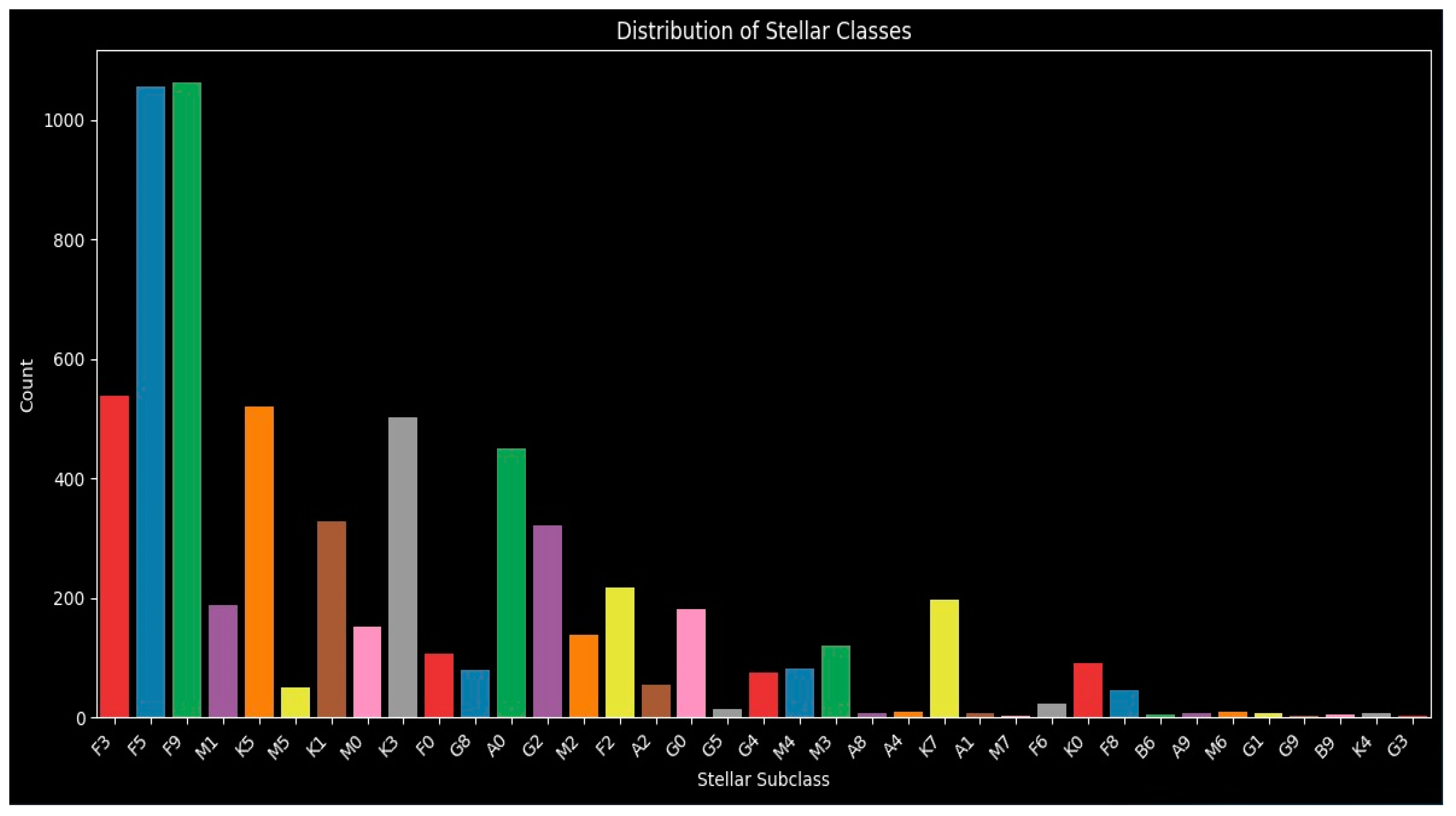
The plot reveals variations in accuracy across different subclasses. Generally, subclasses with a higher representation in the dataset (as seen in Figure 7), such as F3, F5, and M0, tend to show higher prediction accuracies. Conversely, less common subclasses, like G3 and B6, often exhibit lower accuracy. This differential performance per class provides valuable insight into the model’s strengths and weaknesses, suggesting that data imbalance or inherent complexities within certain spectral types may influence predictive capability.
4. Discussion
The results from our tests show that ensemble methods work very well, especially Random Forest, for stellar classification. This technique shows good accuracy, but that is not the only good feature as it is a little resistant to noisy data and high dimension data. The Random Forest model combines the predictions of many decision trees. This combination averages out any oddities, so the model is not likely to overfit the training data set. Thus, this model can detect complex and subtle characteristics of the star data set.
On the other hand, XGBoost is quite interesting. Even though it is used widely and uses boosting, it performed worse in our case. This is likely due to the fact that the trees are added sequentially, one by one, to correct the previous errors. These gradient-boosted systems may get confused if some features have significant overlaps or correlation so that the signature of one class is mistaken for others. Consequently, this indicates that in situations when datasets have highly repetitive features, Random Forest, which constructs trees in a less dependent manner, may be better than boosting.
Visualizations give you a better understanding of the essential features for classification. Some of the photometric indices look quite important, most probably related to some key characteristic of the stars. It emphasizes the use of relevant features that are consistent with the basic stellar characteristics for their classification. These findings are consistent with Flores et al. [Flores], as they also emphasize the importance of relevant features in their stellar spectra models’ classification work.
In terms of a broader picture, the implications of our work in the field of astronomy are quite significant. The success in specific models with minor adjustments, through light application of astronomy knowledge in general, hints as its potential utilization for large-scale ambitious astronomical surveys. It is possible to create a tool to automatically categorize the incredibly vast number of stars present through projects like the Sloan Digital Sky Survey [York], with speed and consistency. Furthermore, the integration of classifications generated by the model with other features such as metallicity, kinematic information, or even spatial distribution could significantly improve our understanding of stellar histories, along with how they are distributed. This particular path is a topic of note in Enis et al. [Cody], where they have also investigated machine learning strategies for classification, specifically using sparser photometric data sets.
By practice, our study opens avenues for future refinement and analysis. One path now is simply trying out a variety of other ensemble methods, such as AdaBoost [Beja-Battais], which assigns varying biases to instances while training, and it may offer new insights into performance gains or the data set. Another critical factor is the necessity to understand hyper-parameter optimization properly. Fine-tuning the settings of the algorithm, precisely one we know does well already like Random Forest, could potentially improve the accuracy of the model even further for specific categorization tasks. In terms of application, computational efficiency is also another critical factor, and so far, the Random Forest model is reasonably fast (10 classifications per 0.3 milliseconds). However, this could still be improved upon by slightly optimizing the decision trees, but not to the extent of a full boosting method.
Something of note is the unexpected results produced. For example, any standard machine learning model might be able to highlight the predictive capabilities of features that may have been unnecessary or deemed secondary by convention but in fact are crucial for improving model performance. In analyzing subtle nuances of features overlooked by traditional analytical methods, we can create new hypotheses regarding the underlying physics of stellar atmospheres or deepen our understanding of these large data sets. The potential for this field is large, and the ideals align with discussions by Flores et al. [Flores] concerning parameter estimation techniques that increase these complex models’ interpretability.
Our investigation into what methodologies are effective for stellar classification and the insights we gained from what ended up performing best is more than just confirming the efficacy of using a machine-learning-based approach. Rather, it is groundwork for future exploration into practical integrations of larger astronomy-related work. Imagine a citizen science platform such as Galaxy Zoo [Madison], where people outsource astronomy work with the assistance and validation of machine learning models. Something like this is the goal, and ultimately, we hope this technology can contribute to our fostered understanding of the universe. Still, the non-stop advancements in applying machine learning to astronomical data sets represent the nature of this field, as highlighted by work like that of Enis et al. [Cody], which underscores the transformative potential of these computational tools in expanding our knowledge and its application.
5. Conclusion
Our study demonstrates widespread effectiveness in the application of machine learning models for the task of stellar classification, a previously tedious and manual task. With an accuracy rate of 76% and a logloss of 0.69, despite being an elementary model, Random Forest Classifier outperformed various other techniques, such as XGBoost, K-Nearest-Neighbors, and Logstic Regressionn. This success highlights the suitability of tree-based ensemble methods for handling noisy data, whilst effectively capturing nonlinear trends in data sets given the right features.
Our methodology employed combining data pre-processing, feature selection, and fine-tuning ensemble learning, which culminated into accurate and automated stellar classification. These findings are particularly valuable for organizations behind the use and creation of astronomical surveys, where large-scale rapid and accurate classification is needed. The model’s reliance on photometric indices and other basic features suggests that there is still more to provide the model with, especially since most data sets contain vast amounts of information provided by things like various telescopes. The analysis established here are also transferable to various other astrophysical problems, such as identifying variable/niche stars like Wolf-Rayet stars [Shenar] or studying galaxy evolution based on stellar clusters.
Our research here isn’t the end, and it underscores the transformative potential of machine learning in astronomy. By using these ensemble methods, along with careful feature engineering, we have achieved the first few steps for progressing in subjects such as stellar classification. The data we have now is only a small portion of the data we will have, and integrating these algorithms and techniques will be crucial for advancing our fostered understanding of the universe.
Acknowledgements
We wish to express our heartfelt thanks to Dr. Mesut Yurukcu, whose expertise, patience, and guidance were invaluable throughout this research process. His dedication to fostering a culture of inquiry and exploration has enabled us to pursue this exciting endeavor.
References
- Ball, N. M., R. J., Data Mining and Machine Learning in Astronomy, International Journal of Modern Physics D, 19(07), 1049-1106. [CrossRef]
- B. F. Guo, Q. Y. Peng, X. Q.Fang, and F. R. Lin. An Astrometric Approach to Measuring the Color of an Object. arXiv:2308.16205 [astro-ph.IM] (2023). [CrossRef]
- Jonathon Shlens. A Tutorial on Principal Component Analysis. arXiv:1404.1100 [cs.LG] (2014). [CrossRef]
- Gilles Louppe. Understanding Random Forests: From Theory to Practice. arXiv:1407.7502 [stat] (2014). [CrossRef]
- Michael J. Madison. Commons at the Intersection of Peer Production, Citizen Science, and Big Data: Galaxy Zoo. arXiv:1409.4296 [astro-ph.GA] (2014). [CrossRef]
- Miguel Flores, Luis J. Corral, and Celia R. Fierro-Santill´an. Stellar Spectra ModelsClassification and Parameter Estimation Using Machine Learning Algorithms. arXiv:2105.07110 [astro-ph.SR] (2021). [CrossRef]
- Moo K. Chung. Introduction to logistic regression. arXiv:2008.13567 [stat.ME] (2020). [CrossRef]
- Pa´draig Cunningham and Sarah Jane Delany. k-Nearest Neighbour Classifiers: 2nd Edition (with Python examples). arXiv:2004.04523 [cs.LG] (2020). [CrossRef]
- Perceval Beja-Battais. Overview of AdaBoost: Reconciling its views to better understand its dynamics. arXiv:2310.18323 [cs.LG] (2023). [CrossRef]
- Sean Enis Cody, Sebastian Scher, Iain McDonald, Albert Zijlstra, Emma Alexander, and Nick L.J. Cox. Machine learning-based stellar classification with highly sparse photometry data. arXiv:2410.22869 [astro-ph.SR] (2024). [CrossRef]
- Tianqi Chen and Carlos Guestrin. XGBoost: A Scalable Tree Boosting System. arXiv:1603.02754 [cs.LG] (2016). [CrossRef]
- Tomer Shenar. Wolf-Rayet stars. arXiv:2410.04436 [astro-ph.SR] . [CrossRef]
- Unknown. HYG Database, Version 4.1, https:// astronexus.com/projects/hyg, licensed under CC BY-SA-4.0.
- Vladimir Vovk. The fundamental nature of the log loss function. arXiv:1502.06254 [cs.LG] (2015). [CrossRef]
- York, D. G., et al., The Sloan Digital Sky Survey: Technical Summary, The Astronomical Journal, 120(3), 1579. [CrossRef]
Figure 1.
Color-color diagram illustrating the relationships between multiple photometric bands. This diagram is fundamental in astrophysics for distinguishing between different spectral classes.
Figure 1.
Color-color diagram illustrating the relationships between multiple photometric bands. This diagram is fundamental in astrophysics for distinguishing between different spectral classes.
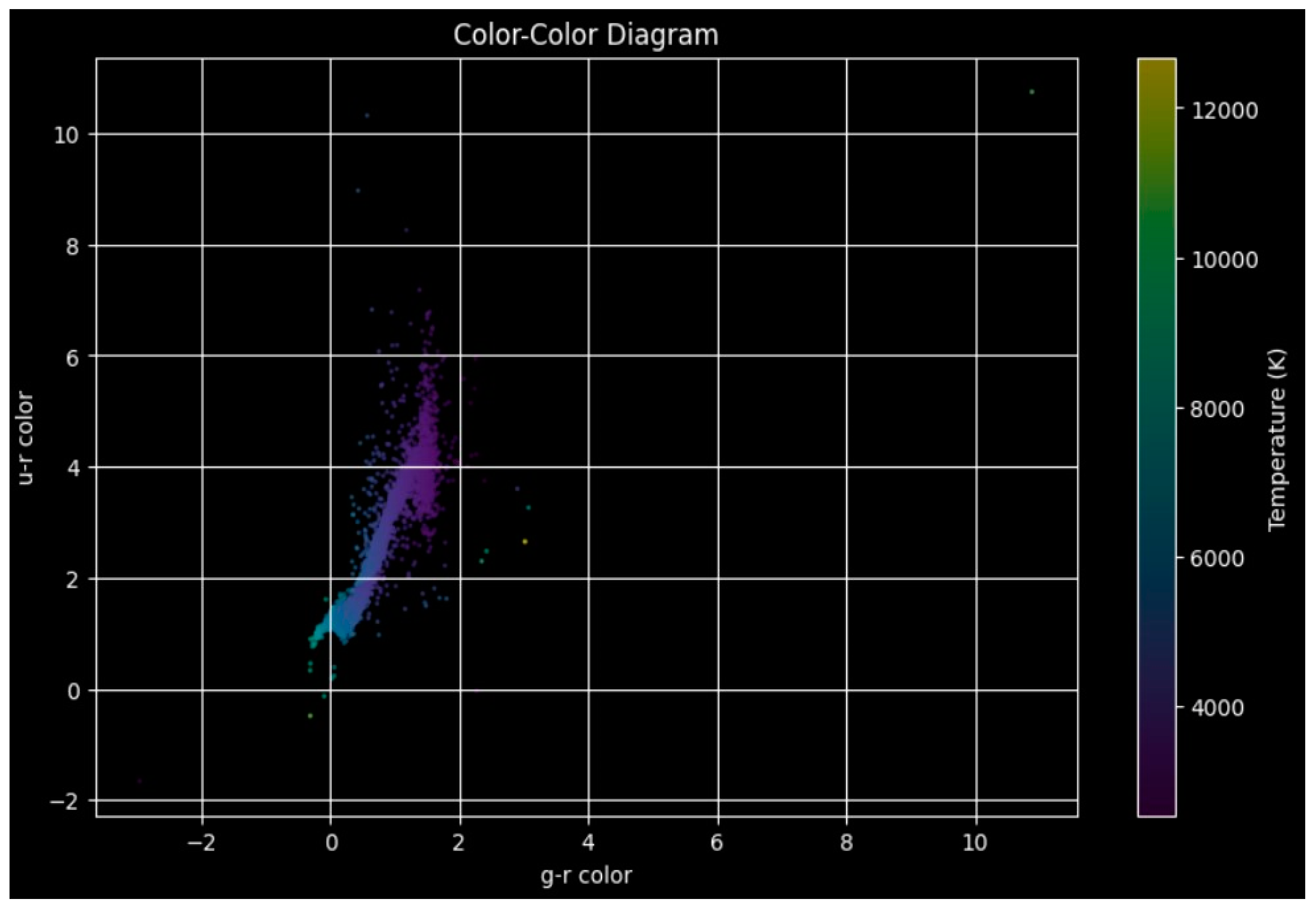
Figure 2.
Three-dimensional plot of color and luminosity space. This visualization helps in understanding the spatial clustering of different stellar classes in a multidimensional feature space.
Figure 2.
Three-dimensional plot of color and luminosity space. This visualization helps in understanding the spatial clustering of different stellar classes in a multidimensional feature space.
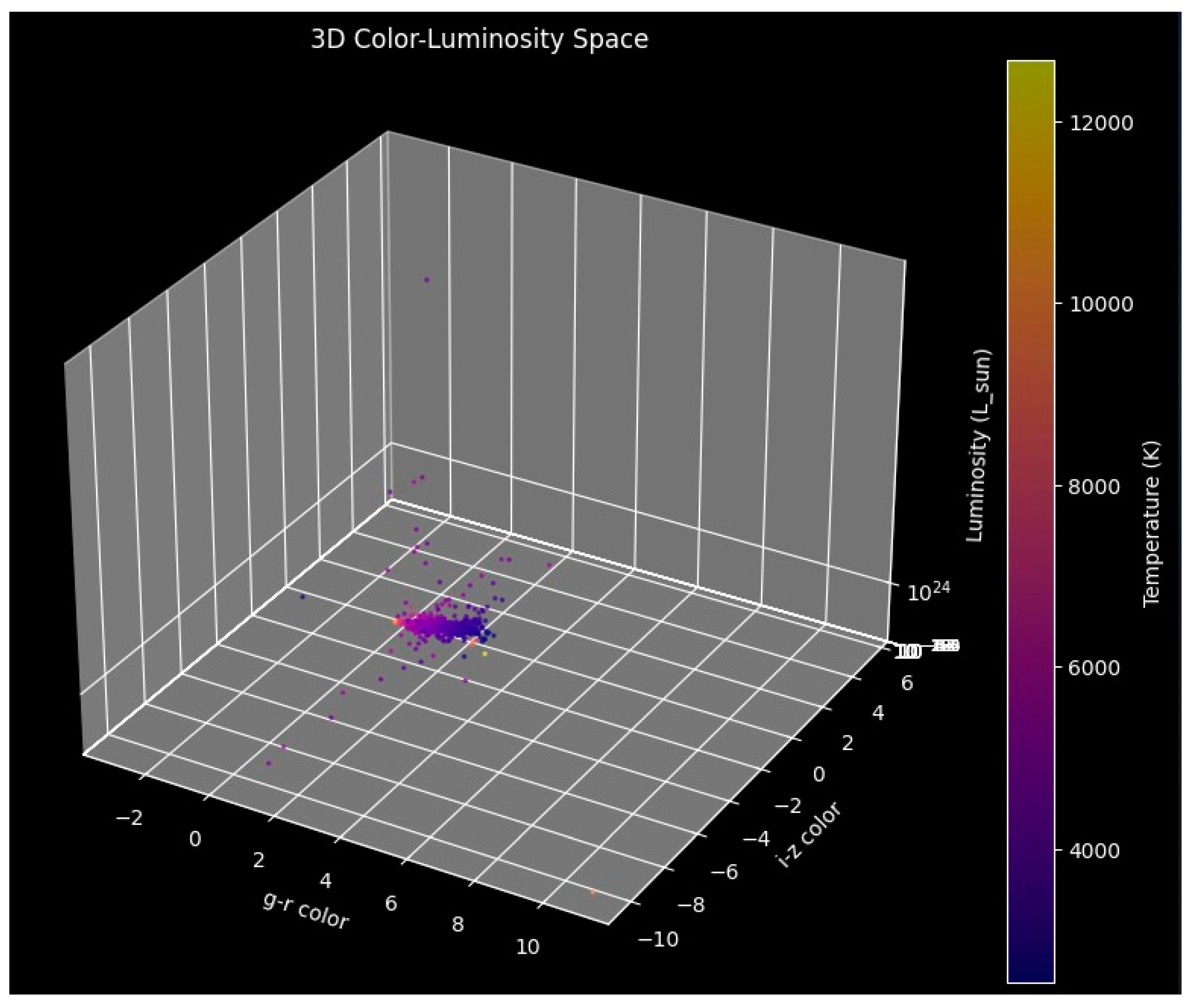
Figure 3.
Accuracy of the Random Forest model for each stellar spectral subclass. This bar plot illustrates the predictive performance of the model broken down by the specific spectral classification of the stars. Our 76% accuracy can be obtained simply by averaging each of these values out.
Figure 3.
Accuracy of the Random Forest model for each stellar spectral subclass. This bar plot illustrates the predictive performance of the model broken down by the specific spectral classification of the stars. Our 76% accuracy can be obtained simply by averaging each of these values out.
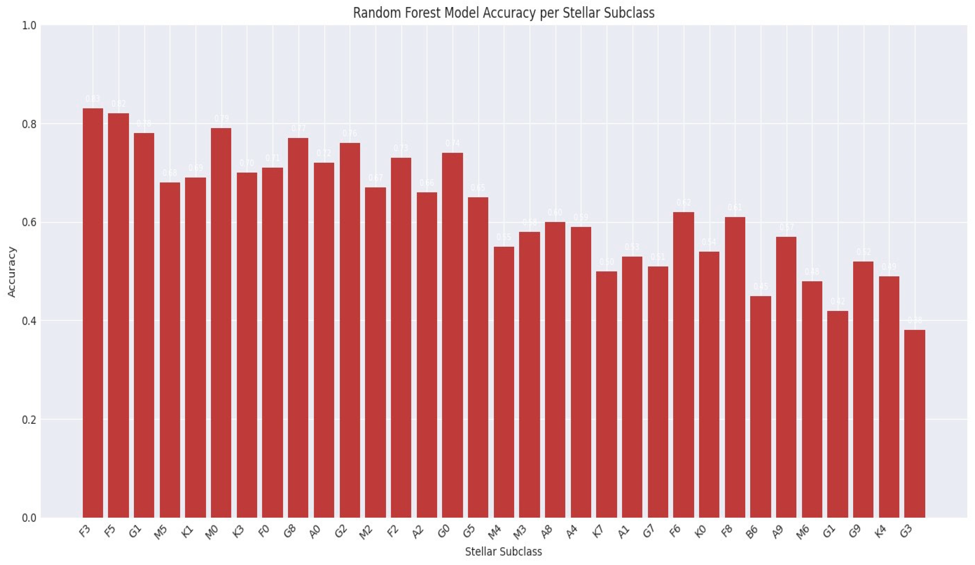
Figure 4.
Correlation matrix plot for all the features. This figure visualizes the pairwise correlations between features, helping identify multicollinearity and guiding further feature selection.
Figure 4.
Correlation matrix plot for all the features. This figure visualizes the pairwise correlations between features, helping identify multicollinearity and guiding further feature selection.
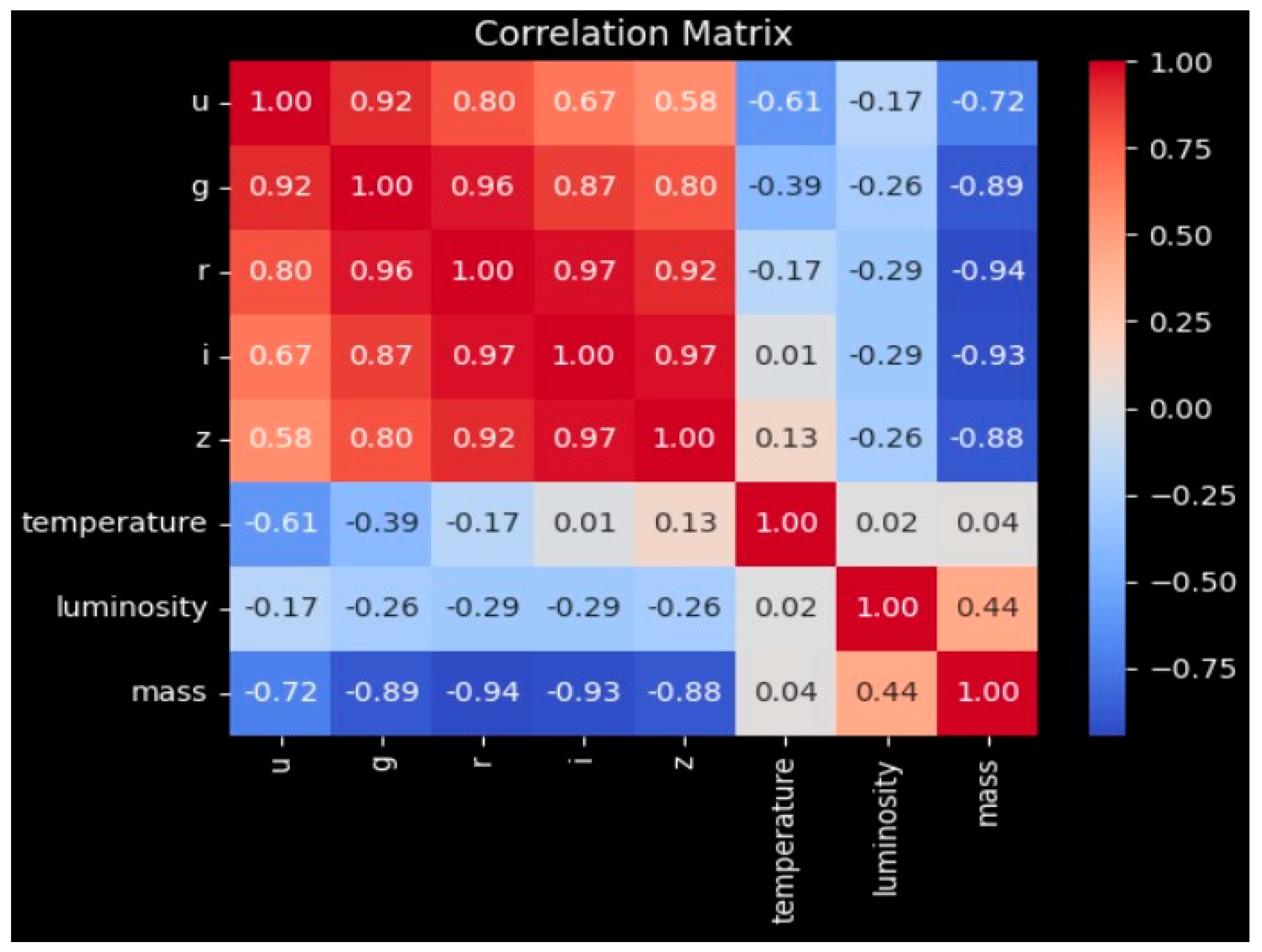
Figure 5.
Feature importance plot derived from the Random Forest Classifier. This figure highlights which features contribute most significantly to the predictive accuracy of the model.
Figure 5.
Feature importance plot derived from the Random Forest Classifier. This figure highlights which features contribute most significantly to the predictive accuracy of the model.
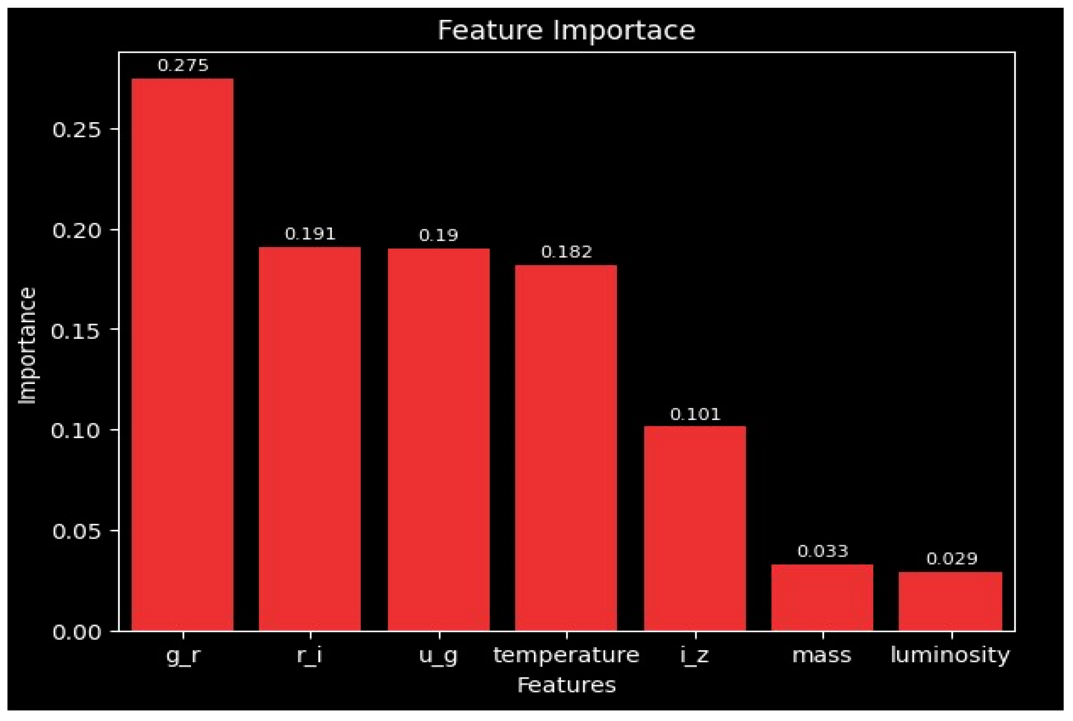
Figure 6.
Cumulative feature importance plot. This visualization aggregates the impact of features in order of importance, showing the cumulative contribution to the model’s predictive performance. Each bar displays its total cumulative importance, and every bar before it, with the bar representing luminosity, also accounts for every other feature.
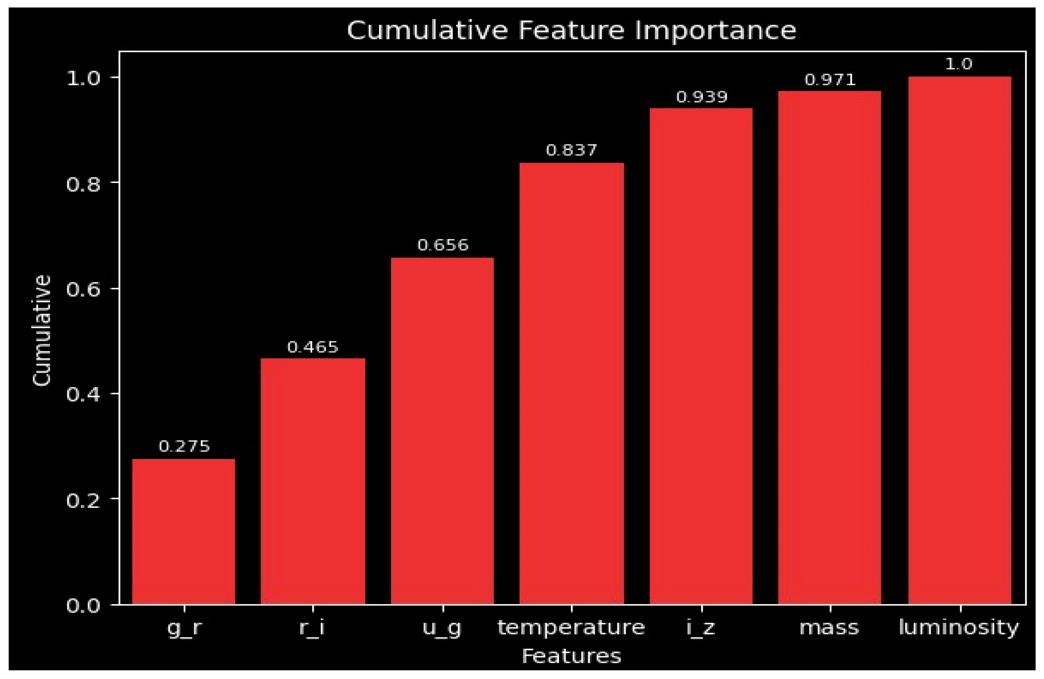
Figure 7.
Feature distribution plot showing the distribution of key stellar parameters. Each letter and number correspond to the type of star, with the height of each bar representing the number of said type of star. This plot helps to identify outliers and the spread of data across crucial variables.
Disclaimer/Publisher’s Note: The statements, opinions and data contained in all publications are solely those of the individual author(s) and contributor(s) and not of MDPI and/or the editor(s). MDPI and/or the editor(s) disclaim responsibility for any injury to people or property resulting from any ideas, methods, instructions or products referred to in the content. |
© 2025 by the authors. Licensee MDPI, Basel, Switzerland. This article is an open access article distributed under the terms and conditions of the Creative Commons Attribution (CC BY) license (http://creativecommons.org/licenses/by/4.0/).
Copyright: This open access article is published under a Creative Commons CC BY 4.0 license, which permit the free download, distribution, and reuse, provided that the author and preprint are cited in any reuse.


