
Submitted:
19 June 2025
Posted:
19 June 2025
You are already at the latest version
Abstract
Quantum computing innovations have garnered significant attention for their potential to revolutionize industries, with the energy sector being one of the most promising 2 areas for application. As global energy demand increases and sustainability becomes more critical, computational technologies offer groundbreaking solutions for energy production, storage, and distribution. In this landscape, quantum computing plays a crucial role in unlocking the full potential of artificial intelligence and machine learning, as the research and development in the quantum machine learning field grows constantly. In this paper, we present a scoping review of early quantum machine learning applications within the energy industry value chain. Starting from 34 sources, we analyze and discuss 22 use cases in the energy sector, thoroughly examining each one to understand its potential applications and impact. We then evaluate these early-stage quantum applications to determine their feasibility and benefits, offering insights into their relevance and effectiveness in the context of the industry’s evolving landscape. This is done by introducing a novel framework: the Assessment Model for Innovation Management (AMIM). Our research highlights the opportunities quantum innovations present for the energy sector and offers actionable insights into which applications are the best investments and why. Overall, the feasibility and technological maturity of quantum machine learning use cases are still in the early stages, though their market compatibility and potential benefits are relatively high for most of them. This indicates that while quantum machine learning holds immense potential, further development is necessary to fully realize its benefits in the energy sector.
Keywords:
quantum computing
; machine learning
; artificial intelligence
; quantum machine learning
; energy industry
; sustainability
; innovation management
; systematic review
; technology feasibility
; industry applications
1. Introduction
The energy industry is undergoing a profound transformation, driven by the increasing complexity of power systems, the integration of decentralized and volatile renewable energy sources, rising global energy demand, and the imperative of decarbonization. These challenges and objectives are reinforced by the dynamics of liberalized energy markets and the need for resilient, efficient, and sustainable operations. In this context, data-driven technologies, particularly machine learning (ML) and artificial intelligence (AI), have become indispensable tools. They support critical functions such as demand forecasting, renewable generation prediction, fault detection, grid stability assessment, and market optimization.
As the reliance on ML grows, so does the demand for computational power and algorithmic efficiency. This is where quantum computing (QC) emerges as a potentially transformative technology. With its theoretical ability to outperform classical computing in a variety of complex computational workloads [1,2,3], such as those found in optimization, simulation, and ML, QC offers a promising path forward. In particular, the field of quantum machine learning (QML) addresses challenging mathematical problems that are crucial to enhance ML tasks, such as classification, clustering, forecasting and others [4].
Although commercially available quantum workloads remain an open challenge, the rapid evolution of quantum hardware and the development of hybrid quantum-classical algorithms have already enabled exploratory studies that could be pivotal for short-term applications. These early efforts aim to demonstrate empirical value using currently available quantum devices or simulators, especially in domains where classical methods face scalability or performance bottlenecks. This review adopts a scoping approach to investigate the emerging intersection of QML and the energy sector. Its primary goal is to identify, categorize, and assess early-stage QML applications that address real-world energy challenges. To ensure accessibility for readers from diverse backgrounds, this paper is structured in two main parts. The following three sections provide essential background information. Section 2 introduces the fundamental concepts of quantum computing. Section 3 outlines the primary machine learning techniques relevant to the industrial applications considered. Section 4 offers an overview of the emerging field of quantum machine learning, with a particular emphasis on the variational approach, currently viewed as the most promising path for leveraging quantum technologies in the short to medium term.
The second part of the paper begins with Section 5, which marks the start of the actual scoping review. This section presents the research questions and details the methodologies employed. It then discusses the findings, focusing on the identification and analysis of early-stage QML applications across various use cases in the energy sector. Finally, Section 6 introduces a novel evaluation framework, the Assessment Model for Innovative Management (AMIM), which is used to assess the selected use cases.
2. Quantum Computing Fundamentals
A quantum computer is a universal computing device that uses quantum bits, or qubits, to store information and execute computations by harnessing the distinctive characteristics of quantum mechanics. This type of computing, known as quantum computing, involves gathering various states of qubits, including superposition, interference, and entanglement, to carry out calculations [5].
In classical computers, the elementary unit of information storage is a bit, which can exist in one of two states: 0 or 1. In contrast, the elementary unit of quantum information is the qubit, which can exist in states represented as and , or in a superposition of these states, denoted as . The states and are referred to as computational basis states, and the Dirac notation "" is the standard representation for qubit states in quantum mechanics. A quantum system with n qubits has a Hilbert space of dimensions, allowing for mutually orthogonal quantum states. For instance, with three qubits, the states can be represented as , , , , , , , .
One of the key features of qubits is superposition, which means that a qubit can be in a combination of both and states simultaneously, described by probability amplitudes and . Specifically, we can represent a qubit as follows:
where and are probability amplitudes of the basis states and , respectively, and both and are complex numbers and satisfy
Upon measurement, the qubit’s state collapses to either or based on the probability of or , respectively.
Another feature in qubits is entanglement, which describes a non-classical correlation phenomenon where two or more qubits cannot be described independently of the state of the others, regardless of the distance separating them. For instance, this means that when two qubits are entangled, a change to one qubit will instantaneously affect the other, even if they are far apart. Moreover, when one entangled qubit is measured, its result contains the information of the other entangled qubits.
By exploiting both features, superposition and entanglement, quantum computers can outperform classical computers in terms of computing power and speed.
The approaches to physically represent and manipulate qubits can be categorized into two main types: analog quantum computing and digital gate-based quantum computing as discussed in the following paragraph.
2.1. Types of Hardware
To apply quantum computing, types of computing systems should be chosen between quantum annealing and quantum gate-based models:
Analog quantum computing In analog quantum computing, the quantum state is smoothly changed by quantum operations such that the information encoded in the final system corresponds to the desired answer with high probability. One example of analog quantum computing is the adiabatic quantum computer [6], which refers to the idea of building a type of universal quantum computing. A special form of adiabatic quantum computers is quantum annealing, which is a framework that incorporates algorithms and hardware designed to solve computational problems via adiabatic quantum evolution towards the ground states of a given quantum system [7]. Quantum annealing takes advantage of the fact that physical systems strive towards the state with the lowest energy, e.g. hot things cool down over time or objects roll downhill. As such, in quantum annealing the energetically most favorable state then corresponds to the solution of the optimization problem [6]. Using the property of superposition and entanglement, the quantum annealer is able to calculate all potential solutions at the same time, which speeds up the calculation process drastically in comparison to classical computers [8]. Due to the nature of their operations, quantum annealers are considered less susceptible to noise than gate-based models. While gate-based computers perform sequential operations, each one affected by a certain amount of noise, quantum annealing leverages the slow evolution of a quantum system towards the equilibrium state, requiring less stringent single-qubit control. Thus, quantum annealing can utilize more qubits and have greater scalability than the quantum gate-based approach. Conversely, quantum annealing is a special-purpose paradigm for optimization problems or probabilistic sampling and no theoretically proven computational advantage has been shown yet.
Digital gate-based quantum computing In digital gate-based quantum computing, the information encoded in qubits is manipulated through digital gates. In comparison to the analog approach in which you sample the natural evolution of quantum states to find the optimal state of low energy, in digital gate-based quantum computers the evolution of the quantum states is manipulated in terms of activity and controlled to find the optimal solution [9]. By actively manipulating the state of qubits, gate-based computing gains a significant advantage in flexibility, enabling such a processing unit to solve a broader range of problems compared to quantum annealing. Indeed, digital gate-based quantum computing is conceptually very similar to classical computation [5]. While a classical algorithm is running on a computer as a series of instructions (gates such as AND, OR, NOT, ... ), quantum gate-based calculators manipulate individual or pairs of classical bits and flip them between zero and one states according to a set of rules. Quantum gates operate directly on one or multiple qubits by rotating and shifting them between different superpositions of the zero and one states as well as different entangled states.
2.2. Quantum Error: Error Suppression, Error Mitigation and Error Correction
A tough challenge in quantum computing is the system’s inherent susceptibility to noise, which causes the degradation of quantum information, a process known as decoherence. This noise manifests in several forms. While the fundamental units at the heart of the quantum processor are highly sensitive to environmental disturbances, the predominant sources of noise are intrinsically linked to the specific physical implementation of the qubits. For instance, superconducting circuits are highly susceptible to thermal fluctuations and stray magnetic fields, whereas trapped-ion systems are more vulnerable to laser instability and electric field noise from trap electrodes [10]. Beyond these technology-specific environmental interactions, noise also universally arises from imprecise control of the quantum hardware or from microscopic manufacturing defects [9]. Since the pervasive and multifaceted nature of these noise sources means they cannot be completely eliminated with current technology, the first era of quantum computers is called the Noisy Intermediate-Scale Quantum (NISQ) era [11]. This term implies that current quantum hardware, which uses dozens of qubits, has high error rates that need improvement before we can build useful quantum computers with hundreds or even thousands of usable qubits. NISQ refers to a class of quantum devices that operate with tens to a few hundred qubits and are subject to significant levels of quantum noise and error. These devices represent the current frontier of quantum computing technology, bridging the gap between small-scale experimental systems and future large-scale, fault-tolerant quantum computers. NISQ devices are characterized by their intermediate size and the presence of noise in their operations. While they are large enough to perform non-trivial quantum computations, they lack the full error correction capabilities required for fault-tolerant computing. This makes them susceptible to errors and limits the complexity and accuracy of the computations they can perform. However, NISQ devices are still powerful tools for exploring quantum algorithms and applications.
Quantum computers today have high error rates – around 1 error occurs in 1000 operations before failure. For quantum computers to be useful, error rates need to be as low as 1 in a trillion. A huge improvement in performance is needed, and proven progress is already happening in the community. We can break error handling into three core pieces, each with their own research and development considerations: error suppression, error mitigation, and error correction:
- Error suppression is a fundamental level of error handling in quantum computing. It involves techniques that use knowledge of undesirable effects to anticipate and avoid potential impacts, often at the hardware level. These methods, which date back decades, typically involve altering or adding control signals to ensure the processor returns the desired result. Error suppression, also known as deterministic or dynamic error suppression, reduces the likelihood of hardware errors during quantum bit manipulation or memory storage. It leverages quantum control techniques to build resilience against errors. For example, quantum logic gates, which are essential for quantum algorithms, can be redefined using machine learning to enhance robustness against errors [12]. Similarly, control operations can protect idle qubits from external interference, akin to a "force field" that deflects noise [13]. Various strategies for error suppression can significantly improve quantum computing performance. Designing new quantum logic gates can make operations up to ten times less likely to suffer errors, thus enhancing algorithmic performance. Research has shown that error suppression can increase the likelihood of achieving correct results by over 1000 times [14]. Error suppression can be integrated into quantum firmware or configured for automated workflows, reducing errors on each run without additional overhead. However, it cannot correct all errors, such as "Energy Relaxation" (T1) errors, which require Quantum Error Correction strategies.
- Error mitigation (EM) is crucial for making near-term quantum computers useful by reducing or eliminating noise through the estimation of expectation values. Each EM method has its own overhead and accuracy level. The most powerful techniques can have exponential overhead, meaning the time to run increases exponentially with the problem size (number of qubits and circuit depth). Users can choose the best technique based on their accuracy needs and acceptable overhead. In quantum computing, estimating calculated parameters, like energy levels of molecules in quantum chemistry, can be affected by errors in both algorithm execution and measurement. Various strategies have been developed to improve results through post-processing, including randomized compiling [15], measurement-error mitigation [16], zero-noise extrapolation [17], and probabilistic error cancellation [18]. These strategies involve running many slightly different versions of a target algorithm and combining the results to "extract the right answer through the errors". Measurement-error mitigation is particularly powerful, using statistical techniques to identify correct calculations despite readout failures. To maximize benefits from EM, an algorithm might need to be run around 100 times with different configurations, which could lead to a significant increase in quantum computing costs.
- Error correction (QEC) aims to achieve fault-tolerant quantum computation by building redundancies so that even if some qubits experience errors, the system still returns accurate results [19]. In classical computing, error correction involves encoding information with redundancy to check for errors. Quantum error correction follows the same principle but must account for new types of errors and carefully measure the system to avoid collapsing the quantum state. In QEC, single qubit values (logical qubits) are encoded across multiple physical qubits. Gates are implemented to treat these physical qubits as error-free logical qubits. The QEC algorithm distributes quantum information across supporting qubits, protecting it against local hardware failures. Special measurements on helper qubits indicate failures without disturbing the stored information, allowing corrections to be applied. QEC involves cycles of gates, syndrome measurements, error inference, and corrections, functioning as feedback stabilization. The entire error-correction cycle is designed to tolerate errors at every stage, enabling error-robust quantum processing even with unreliable components. This fault-tolerant architecture enables the construction of large quantum computers with low error rates, but quantum error correction (QEC) requires a significant number of qubits. The greater the noise, the more qubits are needed, and estimates suggest that thousands of physical qubits may be required to encode a single protected logical qubit, which presents a challenge given the limited qubit counts of current systems. The sheer scale of this overhead and the complexity of QEC is why despite many promising results, QEC still needs further refinement to provide efficient operations for useful applications [20]. This may change soon though, following the recent advancements from hardware providers.
3. Classical Machine Learning: Principles and Overview
Machine Learning (ML) is a branch of Artificial Intelligence (AI) that focuses on building systems that can learn from and make decisions based on data. Unlike traditional programming, where a computer follows explicit instructions, machine learning involves creating algorithms that allow computers to identify patterns and make predictions or decisions without being explicitly programmed to perform the task. The majority of ML algorithms involve training, which means using large amounts of data and an efficient algorithm to adapt and improve based on the training process. After the training phase, the algorithm will be able to apply the acquired knowledge to situations similar to those encountered during training. The advent of Big Data, along with advancements in Internet of Things (IoT) technologies, has exponentially increased the availability of data for training machine learning (ML) models. Nowadays, ML is used to extract meaningful information from these data in a timely and intelligent way. The insights extracted can be used to build various intelligent applications in relevant domains, for instance, to build a data-driven automated and intelligent cybersecurity system, personalized context-aware smart mobile applications, and so on. Machine Learning algorithms are mainly divided into four categories: Supervised learning, Unsupervised learning, Semi-supervised learning, and Reinforcement learning, according to the amount and type of supervision they get during training.
In supervised learning, the training data you feed to the algorithm includes the desired solutions, called labels. The goal of the algorithm is to learn a mapping from inputs to outputs that can be used to predict the labels of new, unseen data. Supervised learning is commonly used for tasks such as classification and regression. The process involves feeding the algorithm a set of training data, allowing it to adjust its parameters to minimize the error between its predictions and the actual labels. Once trained, the model can make accurate predictions on new data based on the patterns it has learned. A classification algorithm divides inputs into a certain number of categories or classes, based on the labeled data it was trained on. These algorithms can handle both binary classifications (e.g. classifying customer feedback as positive or negative, or emails as spam or not) and multi-class classifications (e.g. recognizing handwritten letters, numbers, or categorizing drugs). This versatility makes classification algorithms useful for a wide range of applications. Regression tasks are distinct because they predict a numerical relationship between the input and output data. These models are designed to forecast continuous values rather than discrete categories. For example, they can estimate real estate prices based on factors like zip codes, property size, and market trends. In digital marketing, regression models can predict click-through rates for online ads by analyzing variables such as the time of day, user demographics, and ad content. Additionally, in consumer behavior analysis, these models can forecast a customer’s willingness to pay for a product based on attributes like age, income, and purchasing history.
In unsupervised learning the training data is unlabeled, so the system tries to learn without a teacher, making it a data-driven approach. It is commonly employed to extract generative features, uncover significant patterns and structures, group results, and for exploratory analysis. Typical tasks in unsupervised learning include clustering, density estimation, feature learning, dimensionality reduction, discovering association rules, and detecting anomalies.
3.1. Kernel Method
Kernel methods are a class of techniques used in machine learning to enable algorithms to learn complex patterns in data by implicitly mapping input data into a higher-dimensional space, without explicitly computing the coordinates in that space, a concept known as the “kernel trick”. This allows the algorithm to discover relationships that would be difficult or impossible to model in the original feature space and, also, allows for the linear separation of data that is not linearly separable in the original space. From a mathematical point of view, instead of computing the dot product in the high-dimensional space, we use a kernel function to compute the dot product directly in the input space. Common kernel functions are, for example:
- Linear Kernel — This is just the standard dot product in the original space and doesn’t map the data to a higher dimension.
- Polynomial Kernel — This maps the data into a higher-dimensional space based on polynomial functions.
- Radial Basis Function (RBF) / Gaussian Kernel — This kernel maps the data into an infinite-dimensional space and is often used in SVMs for classification tasks. It is useful for capturing non-linear relationships.
- Sigmoid Kernel — Based on the hyperbolic tangent function, it’s similar to the activation function used in neural networks.
Kernel methods can be used for both supervised and unsupervised learning. In supervised learning, kernels allow algorithms like Support Vector Machines to perform classification and regression tasks in a high-dimensional space efficiently. In unsupervised learning, they find applications in methods like kernel spectral clustering, aiding in the identification of inherent groupings within data.
3.2. Random Forest
Random forest is a commonly-used machine learning algorithm that combines the output of multiple decision trees to reach a single result. Its ease of use and flexibility have fueled its adoption, as it handles both classification and regression problems. Random Forest Classifier works on the Bagging principle, an ensemble technique that starts by choosing a random sample, or subset, from the entire dataset and also a random subset of the input variables. On each subset an individual decision tree is trained, that produces a result. By combining the results of all models through majority voting the most commonly predicted outcome among the models is selected as the final output.
In order to obtain optimal performance from the Random forest, certain conditions must be considered. Firstly, a careful selection of variables should be made in order to avoid the creation of overly correlated decision trees. Furthermore, the number of decision trees to be used depends on the complexity of the problem and the size of the dataset, so that too few trees may lead to an under-robust model, while too many may lead to excessive computational complexity. The depth of the decision trees must also be chosen carefully to avoid overfitting on the training data. Too high a depth can lead to overtraining, while too shallow a depth can lead to an inaccurate model. Finally, the size of the training subset must be chosen so that each decision tree has an adequate number of training examples and sufficient diversity compared to the other decision trees.
3.3. Support Vector Machine
A Support Vector Machine (SVM) is a supervised Machine Learning model, capable of performing linear or nonlinear classification, regression, and even outlier detection. The primary objective of a SVM algorithm is to identify the optimal hyperplane that divides the data points of different classes. SVM tries to find the hyperplane that maximizes the margin, which is the distance between the hyperplane and the closest data points of both classes. These closest data points are called support vectors. The larger the margin, the better the generalization of the model to new data.
In Figure 1 the two classes can clearly be separated easily with a straight line; they are linearly separable. Sometimes, the data is not linearly separable (i.e. no straight line or plane can separate the classes). In this case, SVM uses a mathematical function called a kernel to transform the data into a higher-dimensional space where it becomes separable. If we impose that all instances are clearly separated by the hyperplane, this is called hard margin classification. However, there are two main issues with hard margin classification. First, it only works if the data is linearly separable, and second it is quite sensitive to outliers. So, to find a balance between maximizing the margin and minimizing classification errors you can use the C parameter that controls this trade-off . A small C allows some misclassifications (soft margin), while a large C prioritizes reducing misclassifications (hard margin).
SVMs are potentially designed for binary classification problems. However, with the rise in computationally intensive multiclass problems, several binary classifiers are constructed and combined to formulate SVMs that can implement such multiclass classifications. Moreover, SVM can handle datasets with a large number of features, making it powerful for problems with many variables and they are more robust to overfitting compared to other models. SVMs are particularly well suited for classification of complex but small or medium-sized datasets. For very large datasets, SVMs can be slow to train and may scale poorly, particularly when using non-linear kernels.
3.4. Artificial Neural Networks
Artificial Neural Networks (ANNs) are inspired by the way biological brains process information. In the brain, neurons act as the fundamental units that transmit electrical signals. These neurons are organized in complex networks, with each neuron connected to many others through synapses. They receive inputs, process them, and generate outputs when the accumulated signal surpasses a certain threshold. This behavior is regulated by an activation function, which dictates the output based on the weighted sum of inputs. In a similar way, an ANN is a computational model designed to learn patterns from data. It consists of multiple layers of interconnected nodes (analogous to neurons), where each node performs a mathematical operation on the incoming data and passes the result to the next layer in the network. This hierarchical structure allows the network to learn complex representations from raw data, enabling tasks like classification, regression, and pattern recognition. ANNs rely on various functions to process data, and one of the most widely used is the activation function. A common example is the sigmoid function, also known as the logistic function, which is expressed as:
This function maps the input to a value between 0 and 1, providing a way to introduce non-linearity into the model. This non-linearity is essential for the network to model complex patterns and make accurate predictions, especially in deeper networks.
When ANNs are extended to include many layers of hidden nodes, they form a deeper architecture known as Deep Learning. Deep learning has revolutionized AI by allowing the automatic extraction of complex features from data through multiple levels of abstraction. Deep learning models have been particularly successful in handling unstructured data, such as images, audio, and text, because the additional layers enable them to learn intricate hierarchical features. For instance, in image recognition, early layers might learn to detect edges, intermediate layers might detect textures or shapes, and deeper layers might recognize complex objects like faces or animals.
Training an artificial neural network involves adjusting the model’s parameters (i.e., the weights and biases) to minimize the difference between predicted outputs and true outputs (also known as the loss or error). The goal is to find the optimal set of parameters that best fits the data, a process that requires optimization. The most common optimization method used in training neural networks is Gradient Descent. Gradient descent is an iterative optimization algorithm that updates the model’s parameters in the direction of the negative gradient of the loss function. The gradient represents the rate of change of the loss with respect to each parameter, and moving in the opposite direction helps to reduce the loss. However, basic gradient descent can be slow and inefficient. To address these issues, more advanced optimization algorithms have been developed, including Adaptive Moment Estimation (Adam) and Simultaneous Perturbation Stochastic Approximation (SPSA).
In standard gradient descent, the parameters of the model are updated by subtracting a fraction (known as the learning rate) of the gradient from the current parameter values:
where represents the parameters (weights and biases), is the learning rate, and is the gradient of the loss function .
While effective, basic gradient descent can suffer from problems such as slow convergence and getting stuck in local minima, especially in high-dimensional spaces like those found in deep neural networks.
Adam is an extension of gradient descent that adapts the learning rate for each parameter individually by considering both the first moment (mean) and second moment (variance) of the gradients. This approach helps accelerate convergence and improve stability, especially when gradients are sparse or noisy. Another interesting variant of gradient descent is SPSA. Unlike traditional gradient-based methods that calculate gradients analytically or numerically, SPSA estimates the gradient through perturbations. This makes SPSA particularly useful in situations where the loss function is expensive to compute or when gradients are noisy. In SPSA, rather than evaluating the loss function at each parameter’s current value and its perturbation in each direction, the algorithm performs random perturbations to all parameters simultaneously. This reduces the number of evaluations needed to estimate the gradient, making SPSA more computationally efficient for high-dimensional optimization problems. The general update rule for SPSA is:
where is the random perturbation at iteration t and is the step size or learning rate.
3.5. Restricted Boltzmann Machine
Restricted Boltzmann Machine (RBM) is a type of artificial neural network that is used for unsupervised learning. It is a type of generative model capable of learning the probability distribution of a given set of input data. This neural network comprises two layers of neurons: a visible layer and a hidden layer. The visible layer corresponds to the input data, while the hidden layer captures the features learned by the network. The term "restricted" refers to the fact that neurons within the same layer do not connect to each other. Instead, each neuron in the visible layer is linked only to neurons in the hidden layer, and vice versa. This structure enables the RBM to create a compressed representation of the input data by reducing its dimensionality.
4. Quantum Machine Learning
ML is inherently filled with complexity and large size computational tasks, so that the extraordinary properties of quantum computing have been naturally associated with the ML domain. Hence, Quantum Machine Learning (QML) is one of the most fascinating and promising applications of quantum computing. The concept of QML encompasses a broad variety of methods and algorithms that are still under investigation. Basically, machine learning routines could benefit from quantum computing in two distinct ways: (i) quantum data encoding: systems of qubits constitute the quantum Hilbert space and in principle QML could solve learning tasks much faster by accessing this exponentially large dimension space; (ii) quantum data processing: theoretical computational speedups of several quantum algorithms have been proven and many of them could have high impact in solving certain ML tasks such as sampling, linear algebra, and Fourier transforms [21,22].
Despite the immense potential, there are some limitations of using QML in practical applications, mostly due to the level of maturity of the hardware [11]. The first big caveat is the existence of a Quantum Random Access Memory (QRAM), which is still a debatable topic of research. Many quantum algorithms require a “reading cost” when accessing data and this could even be dominating in the end-to-end computation, neutralizing the speedup during processing. Indeed, QRAM has been already theoretically designed [23,24], and its concrete implementation would enable huge advancements in accessing data directly from quantum hardware. The second challenge is the actual noise when performing quantum computation tasks. The current quantum hardware is characterized by low qubit availability, scarce coherence times and inherent impurities, which leads to noisy results of the computation. This is why one of the main fields of research is how to implement an efficient QEC. Most of the best quantum speedup algorithms require severe error thresholds plus extensive hardware capacity, and this is the first reason that prevents them from being used in real applications.
Indeed, even with the current hardware, the so-called NISQ devices, many near-term quantum machine learning algorithms have been developed. Most of these methods account for a variational approach, that is a hybrid quantum-classical workflow where the quantum processing unit is used only for a specific subroutine, the one that can benefit the most from quantum computing. On the other hand, the rest of the computation, held by classical and/or high-performance computing, is meant to optimize a set of parameters (this is why it is called variational approach) so as to minimize the cost function whose minimum leads to the solution of the problem to be solved. In this respect, one can compare variational quantum algorithms to state-of-the-art Deep Learning models, where a sort of quantum network is optimized via complex parametric tuning, and trained to solve various tasks. Ultimately, there is also another way to quantum machine learning: using quantum-inspired algorithms that employ classical data and classical hardware could still give a certain benefit in the immediate future as a tactical solution [25].
Since the ultimate goal of this review is to give a view on near-term and state-of-the-art applications of quantum machine learning, the following sections are mainly focused on variational quantum algorithms and other “early-available” quantum methods applied to machine learning and their applications to the energy sector.
4.1. Quantum Variational Algorithms
Variational quantum algorithms are based on two essential ingredients: (i) the definition of a cost function(or loss function) that measures how well the algorithm is doing, and (ii) ansatz circuit, which is a set of quantum operations (in a gate-based form) that describes a good solution to the problem, with its tunable parameters adjusted accordingly. Without loss of generality, a parametrized quantum circuit (PQC) ansatz can be expressed by a unitary transformation , where is the vector of the parameters. Essentially, a variational quantum algorithm (VQA) wants to minimise a function as such: . Typically, the “quantum-form" of this cost function can be expressed as:
where C is a function of the parameters, the specific ansatz, and the observable. There are some important guidelines to determine a good choice for a loss function: (i) classically hard to compute but accessible to quantum devices: this is the most important point when seeking quantum advantage; (ii) trainable: there should exist an iterative method capable of finding the global minimum of this function with a certain efficiency; this property is essential in order to guarantee the efficacy of the whole variational procedure.
One fundamental step which is strictly referred to quantum computing principles is the choice of the ansatz . Following the variational procedure, this choice has to be done "a priori", respecting a nice balance between complexity (to express optimal solution) and practicality (to favour convergence). Generally, most of the ansatzes are a sequence of layers, each represented by a product of operators
where is the fixed encoding part and is the actual variational ansatz.
Among the several existing strategies to compute an effective ansatz, there are: (i) hardware-efficient ansatz (HWE), that is meant to be easily run on current, near-term quantum hardware [26]; (ii) problem-inspired ansatz, that is built by leveraging the knowledge of the underlying physics (when present) [27]; (iii) adaptive ansatz, which is specifically designed to adaptively optimize its structure along with that of the parameters [28]. A further notable ansatz is the (iv) quantum approximate optimization algorithm (QAOA) ansatz which, as its name tells, is a particular configuration of quantum gates that alternates between operators derived from an objective function and a mixing Hamiltonian, with the goal of solving combinatorial optimization problems with near-optimal approximate solutions [29].
As far as the classical part of a cost function is concerned, optimal choices of both classical observables and optimization methods have to be done. The first is strictly related to the ultimate objective of the problem (i.e. classification, regression, etc.), so that the observable O is chosen in accordance to the nature of the problem. Secondly, one has to choose among the different options on iterative optimization methods. One effective choice for such differentiable functions is to use gradient-descent loop, which is already widely studied in classical machine learning literature [30].
4.2. Expressivity-Trainability Trade-Off
The most impending challenge for VQAs is the one of the "barren-plateau”: it is rigorously shown that, under mild hypothesis, the average gradient of a random PQCs is equal to zero [31,32]. Not only this, but the gradient variance of a random PQCs decays exponentially with the number of qubits [33]. This problem is also called “vanishing gradient” and could be really detrimental especially in the regime where qubits are much more than 1, which is, by contrast, when one would expect the most quantum advantage. Fortunately, there are many mitigation strategies [34,35,36]. All of them are basically focused on moving away from the vanishing gradient initial hypothesis of a "universal", random unitary that leads to maximum expressivity but difficult trainability at the same time. The idea is to have an ansatz where complexity is controlled to address specific, problem-inspired expressivity. Thus, trainability is preserved and efficiency optimized.
Another way to improve trainability compensating for the vanishing-gradient phenomenon is to work on classical optimization methods: one can either operate on optimizers like Adam or SPSA algorithms or employ a varying learning rate over training. Furthermore, since the appearance of the barren-plateau is strictly related to the variational parameter initialization [37], techniques like the so-called “warm-start” have been successfully employed to adjust parameter initialization in a pre-training phase [38]; similarly, one strategy is to optimize a subset of parameters at a time in a layer-wise approach [39]. Another completely different approach is to work without a call to a classical optimization algorithm: for any variational cost function that is a linear sum of expectation values, an exact formula can be extrapolated to find one optimal parameter at a time that guarantees a decreasing behavior of the cost function over training [40].
In summary, the problem of barren-plateau is a critical topic for near-term quantum ML applications and although there is no universal solution available, there are many mitigation strategies that depend on the specific case that can be adopted.
4.3. Explicit Quantum Models
Suppose we are given a set of classical data points , where each . The first fundamental step in implementing a Variational Quantum Algorithm (VQA) is the so-called feature embedding, where classical data are mapped into the quantum Hilbert space. This is achieved via a parameterized unitary transformation , which encodes the classical input into a quantum state:
Here, denotes the Hilbert space of an n-qubit quantum system, which has dimension . The state is the quantum feature representation of the classical input x. The operation can be chosen among different alternatives [41]. The most frequently used are: (i) amplitude embedding: encodes a normalized N-dimensional feature vector into a quantum state of n-qubits. This is done by putting the normalized data as amplitudes of a quantum wavefunction:
where is the i-th element of x, and is the i-th computational basis state; (ii) angle embedding: encodes a n-dimensional sample into an angle rotations applied to as many qubits
Single gate operations as Pauli rotations are Pauli rotations (2.6) around one of the Pauli axis are parametrized by the input values and then used to map the resulting quantum state; (iii) basis embedding: encodes a N-bit binary string input with into a quantum state of N qubits. This is achieved by simply mapping the bits to a corresponding computational basis state, with the formula:
From these three different approaches, many variants have been developed [40,42,43]. Balancing robustness with as few qubits as possible is crucial to address real problems with the near-term hardware availability. After the encoding phase, the variational unitary is applied. The resulting quantum state follows:
Then, the last step of an explicit quantum model is to compute an observable at the end of the quantum computation:
This observable is directly used in the loss function of a supervised machine learning model, i.e. a classification or a regression problem [44,45], to drive the training procedure. Notably, the optimization of the variational parameters is implemented by directly measuring the observable on a quantum computer.
4.4. Implicit Quantum Models (Quantum Kernels)
Similarly to classical Kernels (discussed in Section 3.1), Quantum Kernels can be defined [46]. These methods (often called implicit models) work as the classical framework where now the Kernel function is given by the inner product in the quantum feature space:
Thus, quantum computers can be only used to compute the Kernel function, whereas the variational parameters that define the optimal model as a linear combination of kernel evaluations are purely classical. This quantum kernel estimation (QKE) has been first proposed by Maria Schuld and Nathan Killoran [47]. Shortly after that, a subsequent work proved that there exist classically intractable kernels that can be accessed with the use of the quantum feature space with a theoretical exponential advantage [44]. From that on, several quantum circuits have been proposed to calculate quantum kernels applied to machine learning models. Particularly, quantum kernels can be used within regression or classification tasks as, for example, quantum support vector machines [48,49]. Notably, as for their classical version, implicit models are guaranteed with the best performance by the representer theorem [50]. On the other hand, they require queries to the quantum computer where m is the number of samples in the training dataset, plus an additional classical-processing queries to compute the optimal Kernel weights for the optimal predictor [51]. By contrast, explicit models need calls to the quantum computer, where p is the number of variational parameters that have to be tuned. Evidently, when there is no need to have a large number of parameters to describe the variational block , explicit models are cheaper and therefore more efficient than implicit ones. By contrast, quantum kernels are proven to guarantee advantage under specific, complex conditions.
4.5. Quantum Neural Networks
Explicit and implicit models have in common the fact that they can be mathematically treated as an inner product between a data-dependent quantum state (or feature map) and a trainable observable [52]. This property gives the previous methods a linearity framework to lay on. When this linearity is broken, similarly to what happens in classical machine learning, we enter the realm of quantum neural networks (QNN). Differently from the two previous approaches, a quantum neural network is defined when a parametrized quantum circuit uses a repeated structure of both encoding and variational layer, assuming the form:
where L is the number of layers of the QNN. The fundamental property of this form of unitary is to add "data re-uploading", that is the repeated use of input data in the unitary computation via multiple encoding layers. Notably, although the name recalls the classical neural network framework due to its layered structure, Quantum Neural Networks (QNNs) differ significantly in both approach and underlying mathematics. Theoretically, this type of PQC has been shown to correspond to an L-truncated Fourier series when angle-embedding is employed [53]:
where is a finite set of frequency vectors. Such formalism is very helpful because it gives a way to characterize QNN generalization performance by the use of already known statistical concepts. Essentially, it has been proven that the Generalization Error (GE) of a QNN can be bounded as [54,55]:
where is the Fourier spectrum of frequencies accessed by the QNN and m is the training data size. Notably, when is too large (which means a high complex quantum circuit), the model weakens in such a measure that only a corresponding increase of data size is able to compensate. This consequence is something one has to take into account when designing a QNN. Given that, several studies of practical applications have shown a practical advantage in terms of expressivity of QNN when compared to classical versions of the same size, raising interest on the topic [43,56,57]. Of particular importance is the fact that QNN structure can be integrated in classical NN architectures, forming hybrid quantum-classical neural networks. This approach allows a greater scalability when large datasets are employed, that is basically the case for almost every real-world scenario. For instance, deep learning and VQA can be trained and run in parallel where classical NN layers can be used to further reduce the input data dimension so that VQA’s employment is enabled with the current quantum hardware available. Although there can be no analytical proof of the effectiveness of the quantum integration in such hybrid structures, applications of hybrid QML are widespread in literature with evidence of empirical advantages over purely classical counterparts [58,59,60].
4.6. Quantum Annealing Applied to Machine Learning
Indeed, apart from the variational approach employing gate-based hardware, there are alternative “quantum” ways to enhance classical machine learning performance, one of them being quantum annealing. Since Machine Learning is filled with optimization problems, quantum annealing processors have become popular in solving some of these optimization tasks in machine learning applications. One of the first and most popular fields of application for QA is feature selection, that is the process of extracting the most efficient subset of features from input data of ML models. This is a complex decisional problem that can be solved with Ising-like models run on annealers. Quantum hardware is therefore potentially helpful when dealing with wide and complex datasets [61]. One other interesting use of QA is the optimal sampling of data to train random forest (RF) classification models [62], which has been proven able to increase classification accuracy of the purely classical RF. Furthermore, a popular quantum-enhanced deep learning model is the restricted Boltzmann machine (RBM) Figure 2. Quantizing the classical version of the RBM is simple: one has to take the network and express it as a set of coupled spins, resembling the Ising model. Then, the last one can be solved using QA, obtaining the optimal, tuned network. Quantum RBM models have been successfully implemented in a real-scenario classification problem with interesting results [63,64].
5. Case-Based Research in the Energy Sector
5.1. Rationale
Electricity is arguably the most important energy resource of modern society. Among the essential daily activities that depend on electricity one can name healthcare services, communications, information technology, house devices usage, and many more. All this is guaranteed thanks to a reliable and continuous supply from power plants. The major stages of a power plant process are: generation, transmission, distribution. Today electricity operators companies are facing old and new challenges to keep up with society’s needs. On one hand, the global energy demand is destined to increase, requiring the extension of existing power supply systems. On the other hand, environmental impact must be taken seriously into account, shifting to more sustainable processes. One (if not the only) viable solution is the adoption of key-enabling new technologies, capable of dealing with today’s increasing complexity but rooted on sustainability as a paradigm. Among these, one of the most important is undoubtedly artificial intelligence, whose efficacy is determined by machine learning algorithms and high-performance computation. That is why SPOKE 10 of NextGenEU program of funds, managed by Politecnico di Milano, is dedicated to high performance and quantum computing (HPC and QC) [65]. QC is particularly interesting for its disruptive potential in the energy and utilities (E&U) industry, which is filled with computational complexity. In particular, forecasting problems are crucial to establish efficient power supply operations and they mostly rely on ML. Fortunately, as exposed in previous sections, QC in its theoretical framework suits nicely with ML. Although the spectrum of quantum machine learning applications for E&U is even broader than the following review, the focus of this work is on quantum applications for the energy industry that can be practically assessed with today’s technology maturity. The reason for this pragmatic approach is two fold: first, the objective is to shed light on early opportunities for quantum technology adoption in a reasonable horizon of time; secondly, only when real hardware faces real problems the actual capabilities of a new technology are really explored. With this in mind, we formulated two research questions:
- How can the energy and utilities sector benefit from quantum computing, and which specific ML applications or challenges will QC address in the near- to medium-term future?
- Which use cases of quantum machine learning have the most significant impact on the energy and utilities sector related to their level of readiness?
5.2. Methods and Overview
To answer the questions above, the Preferred Reporting Items for Systematic Reviews and Meta-Analysis extension statement for Scoping Reviews (PRISMA-ScR) has been followed [66]. The adopted protocol is presented in the reported flow diagram (Figure 3). As databases sources, we employed Scopus and WebOfScience. We searched for documents containing combinations of the following terms: ((energy AND generation) OR (demand AND response) OR (solar AND irradiance) OR (solar AND irradiation) OR (wind AND speed) OR (eolic AND power) OR (photovoltaic AND power) OR (solar AND power) OR (wind AND power) OR (wind AND farm) OR (fault AND detection) OR (defect AND detection) OR ("smart grid") OR ("power systems") OR (carbon AND market) OR (energy AND market) OR ("smart cities") OR ("smart building") OR ("smart home*") OR ("smart meter*") OR ("high-voltage grid*") OR ("high-voltage power line*")) AND (("quantum support vector machine*") OR (hybrid AND quantum-classical AND computing) OR (hybrid AND classical-quantum AND computing) OR ("quantum neural network*") OR ("quantum reinforcement learning") OR ("quantum machine learning") OR (quantum AND variational AND computing) OR (quantum AND convolutional AND network AND computing) OR (quantum AND computing AND kernel) OR (quantum AND computing AND hybrid AND deep AND learning) OR (quantum AND long-short AND memory AND network)).
This query combines the two thematic fields of the scoping review: energy systems and infrastructure, and quantum machine learning. It was applied to the title, abstract, and keywords fields of the documents. Filters were set to include only documents published before 2025, written in English, and classified as either articles or conference papers. In addition to that, as a secondary source, a raw search has been conducted on Google Scholar archive, using the most frequent keywords, such as: ’energy’, ’energy generation’, ’energy transmission’, ’energy distribution’, ’power systems’, ’quantum machine learning’, ’quantum neural network’, ’quantum support vector machine’. A total of 265 records have been identified from databases. Duplicates were first removed automatically using MSExcel similarity function, resulting in 209 records. These were screened on titles and abstract and eventually reviewed on full-text for the ultimate eligibility. These screening operations have been conducted by the first and the second authors independently, followed by a sharing session for the final decision on each item. Separately, other authors proceeded with the Google search. Their results were filtered if already present in the screening from the primary sources. From that, 35 items required further investigation. Plus, from the full-text screening, 11 citations were identified in scope. Therefore, we gather the ultimate collection of key studies applying specific inclusion and exclusion criteria. As inclusion criteria, there have been the following: (i) the application involves one or more computational problems of the energy industry value chain; (ii) the algorithm implies a machine learning technique; (iii) the quantum computing solution proposed is viable in the NISQ era of quantum computers, which include gate-based variational approach, hybrid architectures and quantum annealing. We have also implemented the following exclusion criteria: (i) employment of general-purpose quantum algorithms that imply scaled fault-tolerance quantum computers (i.e. Grover algorithm, HHL, etc.); (ii) the absence of a real test on datasets referred to the energy industry or related applications; (iii) quantum-inspired approaches. At the end, 29 sources were included from databases and 5 sources were included via the secondary source or citation.
Key studies that have been charted in table "Use Case Method’s Overview" (Table 2) clearly suggest that quantum machine learning has the potential to be applied to a wide range of applications in the energy industry. The number of total articles reviewed is 34 (see Table 1). The main source of articles is the USA, followed by China. At the continental level, Asia contributes the highest overall number of publications. Nine main categories of applications have been identified which belong to a piece of the energy industry value chain: demand response systems, smart grid management, indirect generation forecasting, direct generation forecasting, plant operations, grid maintenance, grid operations, finance for sustainable energy, smart energy distribution. A set of descriptive features of these works has been extracted: (i)method, that is the specific name that authors gave to the quantum model they use; (ii) typology, which is a closed choice between the five categories of quantum computing methods reviewed in chapter 4: 1. Explicit VQA; 2. Implicit VQA (or Quantum Kernel); 3. Data re-uploading (or QNN); 4. Hybrid (mix of PQC and classical workloads in a single model architecture); 5. Annealing (or analog quantum computing); (iii) software technology, that is the reference (when present) of which cloud platform/SDK/libraries have been used for the application; (iv) hardware technology, that is the reference of which QPU has been used (we indicate the simulator in case of no QPU employed).
As one can see from the following figures (Figure 4 and Figure 5), the elements of the value chain with the highest number of studies are related to "Generation" and "Transmission", which suggests that these are ones of the most valuable topics for the industry. Additionally, data collection for energy generation use cases is made easy by the availability of transparency data on energy generation from plants and weather data. Nonetheless, given that many different methods of generation forecasting are employed for the same application, the energy "Transmission" element of the value chain is the one with most distinct use cases. This value chain is indeed very rich in applications and, additionally, its use cases are often the most impactful of the energy industry businesses, with major consequences for society and final users.
5.3. Distribution
5.3.1. Overview
Predicting energy demand with reasonable accuracy is arguably one of the oldest and most important challenge for a power system supply chain. Modeling future information on energy demand is a rich and wide field of research. First of all, energy demand forecasting methods can be categorized by two essential features: spatial and temporal resolution. The former describes models ranging from single appliance to country-level energy demand, while the latter varies from sub-hourly energy request to yearly energy consumption. More local and responsive forecasting is crucial to daily demand-response operations in power grids and day-ahead energy markets. In turn, more aggregated and long-term information are useful for strategic planning and decision making. There are several specialized reviews that cover the range of existing techniques for energy demand estimation [101,102,103,104,105], which we refer to for an extensive view on the topic. Here we mention the most important criteria of an energy forecasting method: spatial resolution, temporal resolution, input features, data preparation, data size, applied techniques, forecasting horizon, metrics of performance. In the following the focus will be on the range of the applied techniques, starting from classical and conventional methods and eventually reaching the use of quantum computing.
The simplest classification of load forecasting techniques in literature is to divide them between conventional techniques and machine-learning-based techniques [106]. The former class involves statistical methods, subdivided in Time Series Analysis (TSA) and regression methods. TSA techniques consist in using the historical time series of data to infer future predictions. Popular TSA models are Autoregressive Moving Average Analysis ARMA and ARIMA, that is its version for non-stationary time series [107]. On the other hand, regression models are meant to find a functional relation between inputs and outputs of a system, by minimizing a cost function that is typically a figure of optimal fitting between data points and the regression wave of predictions. In the case of the linear relation hypothesis, the cost function is the sum of the squares of the residuals, that are the difference between observed values and the fitted ones [108]. Then, non-linear functional relations can be assumed with the use of more complex cost functions or implementations of Kernel methods [109]. An advancement from regression methods are machine learning models. NN and SVM are the most employed ML models to derive the function that relates input data to the energy load demand historic output. Once this relation is trained, learned and validated, current input data are fed to the model so that future energy demand can be efficiently predicted. In the category of ML-based techniques one also has Decision Trees (DT) [110], Bayesian [111] and ensemble learning [112] approaches. Other than conventional and ML-based techniques, there are also other alternative methods applied to energy demand forecasting. One of them is the employment of metaheuristics combined to ML: genetic algorithms, particle swarm optimization and other similar algorithms can be used to optimize parameters search in SVM or NN models [113]. Furthermore, stochastic processes can be employed to simulate load profile, using Markov chains [114], while more advanced techniques based on probability theory like fuzzy logic and grey systems are a good way to develop uncertainty aware forecasting models [115,116].
5.3.2. Key Studies
QML is an interesting perspective for more accurate and resolute energy demand forecasting. In their work, Kumar et al. discuss the application of Quantum Support Vector Machine (QSVM) in forecasting energy consumption within Home Energy Management Systems (HEMS) in smart grids [67]. The authors highlight the importance of accurate load forecasting to manage energy consumption efficiently, which is crucial due to the fluctuating energy demands in households. The study compares QSVM with traditional deep learning models like Recurrent Neural Networks (RNN) and Long Short-Term Memory (LSTM) networks, demonstrating QSVM’s superior performance in handling complex and nonlinear electricity consumption patterns. Their methodology involves using the AMPds2 dataset, which contains data on various household energy loads. After data pre-processing and normalization, a quantum kernel is computed using 2, 4 and 8 qubits. Angle embedding and ZZ feature map [117] as circuit ansatz are employed to model the kernel function. Once computed, the quantum kernel is used for an SVM conventional training. The results on testing data show that QSVM achieves a higher accuracy of 97.36% compared to the deep learning models, which have slightly lower accuracies. This is attributed to QSVM’s ability to efficiently process large datasets and capture intricate relationships within the data. This outcome emphasizes QSVM’s potential as a promising solution for enhancing forecasting accuracy in HEMS, suggesting that future research could explore its adaptability to different datasets and its performance in real-world scenarios. The study also proposes the development of hybrid models that combine multiple forecasting techniques to further improve prediction accuracy.
More recently, Safari and Badamchizadeh introduced NeuroQuMan, a cutting-edge approach that combines quantum computing and machine learning to enhance energy management systems [68]. This innovative method employs a three-Qubit Quantum Neural Network (QNN) to predict energy demand based on user reaction times, aiming to optimize energy consumption and improve grid stability. The structure of NeuroQuMan involves several key components: data preprocessing, quantum device initialization, quantum circuit definition, user decision-making, QNN predictions, and visualization of results. The process begins with preparing real-time data, such as reaction times and power outputs, for analysis. A quantum device is then initialized to execute quantum circuits, which are defined using specific quantum operations. These circuits simulate user decision-making and optimize power generation through economic dispatch calculations. In detail, the architecture followed the typical structure of a variational QNN: firstly, a quantum data encoding of response times, energy loads and power generated was performed via 3-qubit angle embedding. The actual scheme of a variational quantum circuit is then iteratively applied using quantum gates. Finally, the output is measured from the final quantum state. The QNN model predicts demand and renewable energy generation, with the results visualized to assess performance. The results from simulations show that NeuroQuMan achieves significant accuracy in predicting demand response, with metrics like RMSPE and MAPE indicating its effectiveness. The model’s performance is compared with other methodologies, demonstrating its superior accuracy and efficiency. Despite its promising results, NeuroQuMan faces challenges such as the limitations of current quantum hardware and the complexity of quantum circuit design. Future work aims to integrate advanced quantum machine learning techniques, like Quantum LSTM and Quantum Neuro-Fuzzy systems, to further enhance prediction accuracy and manage uncertainties in energy systems.
Concerning hybrid architectures, a proper work from Ajagekar and You [69] discusses a cutting-edge approach to managing energy consumption in buildings using a hybrid quantum-classical control framework. This innovative strategy leverages the strengths of both quantum and classical computing to enhance demand response, which is crucial for reducing energy use and carbon emissions in grid-interactive buildings. The study’s primary objective is to develop a robust control system that can efficiently manage energy demands in buildings equipped with renewable energy sources and storage devices. By using variational quantum circuits (VQCs) within a reinforcement learning framework, the system can make real-time decisions to optimize energy use. This approach addresses the limitations of traditional methods, offering improved scalability and performance as the size of building microgrids increases. This controller is formulated as a markov decision process and is based on three main components: (i) estimation of the value function using VQC: the VQC is used to approximate the value of the state-action function for a state and control pair . In a reinforcement learning context, the value function represents the cumulative sum of discounted rewards over an infinite horizon; (ii) extraction of controls from a trained VQC: after the VQC has been trained, it is used to extract the necessary controls to manage energy storage devices and optimize the energy consumption of buildings; (iii) integration of quantum and classical routines: this enables circuit learning and the calculation of optimal control. The VQC consists of three main components: first, an amplitude encoding scheme responsible for translating a classical data into a quantum state. Then, parametric gate operations are applied to the input quantum state to manipulate it according to the trainable parameters of the VQC. These are obtained by combining an entangling layer composed by CNOT gates, single qubit Pauli rotations, and lastly the pooling operator is applied, comprising a sequence of operations between a source and sink qubit pair, like sink qubit inversion along z-axis, inverted CNOT among the two, plus fixed amount rotations along z- and y-axis. Ultimately, the circuit learning phase measures the resulting quantum state with an observable to estimate the objective function. Learning the function is formulated as minimizing a loss function, and a gradient descent algorithm is used to update the parameters of the variational circuit. The results of the study are promising, showing that the hybrid VQC-based strategy can reduce energy consumption and carbon emissions by over 13.6% compared to classical methods like deep deterministic policy gradient and model predictive control. The framework is designed to be adaptable, handling uncertainties such as fluctuating renewable energy generation and varying carbon intensity levels. The hybrid approach is proven to be a valid way to enhance computational efficiency and address scalable solutions for current quantum hardware. This work underscores the importance of quantum-classical integration of architectures, combining quantum workloads with classical optimization to tackle complex and critical real-world challenges like adaptive response to energy demand.
Another work on quantum reinforcement learning is proposed by Andrés et al. [70]. The document outlines a methodology for training RL agents using a hybrid classical and quantum approach. The primary focus is on the design and training of agents in an environment called Eplus-demo-v1, utilizing the Advantage Actor-Critic (A2C) algorithm. Eplus-demo-v1 simulates a heating, ventilation, air-conditioning HVAC scenario in a target building, while the RL algorithm’s main objective is saving and optimizing energy demand. The methodology involves two distinct types of experiments: one using a classic feedforward Multi-Layer Perceptron (MLP) neural network and the other employing a hybrid architecture that combines a linear layer with a Variational Quantum Circuit (VQC). In the classical approach, the MLP neural network is used to model the agent’s policy. This network is trained using the A2C algorithm, which is a popular method in RL for learning stochastic policies. The training process involves running four environments in parallel to generate batches of interactions between the agent and the environment. A discount factor of 0.98 is used to calculate the total return of each episode, and the training is set to stop after 100 episodes. The agent’s performance is evaluated in the final episode using a deterministic policy that selects the action with the highest probability. The quantum approach involves designing a quantum agent with a hybrid architecture. This agent also uses the A2C algorithm for training, maintaining the same settings as the classical agent to ensure a fair comparison. The quantum agent’s policy is implemented with a variational quantum circuit, which is integrated with a linear layer. This configuration aims to leverage the potential advantages of quantum computing, such as reduced parameter space and computational complexity, while still utilizing classical neural network components. The authors also discuss the structure of the networks used in the experiments. For the classical MLP networks, the number of parameters is significantly larger compared to the quantum VQC networks. The quantum networks have a reduced number of parameters, which is expected to decrease the computational complexity of the simulations. The methodology emphasizes the use of separate networks for different action sets, which helps manage the computational demands of simulating quantum neural networks. The results highlight the total accumulated rewards obtained by both quantum and classical agents. The VQC agent consistently converges to the optimal policy, achieving the same value for average, best, and worst total rewards, as well as in test episodes using a deterministic policy. This consistency indicates that the VQC agent effectively learns the optimal policy. In contrast, the MLP agent does not reach the optimal policy, with its best execution yielding worse total and average rewards across all executions. However, the authors also note a limitation of the quantum agent, which is the high computational time required to simulate the quantum environment.
Arvanitidis, Valdez, and Alamaniotis (2023) [71] present research on the precise identification of electrical appliances within smart grids using power consumption data, a task crucial for efficient energy management, demand response programs, load monitoring, and potentially electricity theft detection. The study specifically investigates and compares the performance of a classical Convolutional Neural Network (CNN) against a cutting-edge Variational Quantum Classifier (VQC) for this classification task. The VQC’s operation is described in three stages: firstly, data encoding is performed using Z-feature maps, which utilize rotational quantum gates to map classical consumption data into a higher-dimensional Hilbert space. Secondly, an Ansatz variation model is constructed, characterized by two entangled parameterized rotational gates; the parameters of this Ansatz are optimized using the COBYLA optimizer. The third stage involves quantum measurement, where the resulting probability distribution across basis states is mapped using a parity post-processing method to yield a classification outcome. As a classical benchmark, a "robust Convolutional Neural Network (CNN)" is used; its architecture includes a 1D convolutional layer (32 filters, size 3, ReLU activation), followed by a 1D max pooling layer, a flatten layer, and an output layer with 7 neurons corresponding to the appliance classes. The study utilized a subset of the 2017 Plug-Load Appliance Identification Dataset (PLAID), which contains voltage and current measurements from seven different household appliances collected from 65 distinct locations in Pittsburgh, Pennsylvania. The findings indicate that the proposed VQC demonstrated superior performance in this challenging classification task. The VQC achieved an accuracy of 0.81 and a Cohen’s kappa score of 0.745, while the CNN achieved an accuracy of 0.755 and a Cohen’s kappa score of 0.713. This represented an approximate 5% enhancement in classification results by the VQC. However, the authors note a significant trade-off: the training convergence time for the VQC model was considerably longer than that of the CNN, primarily due to the computational expense of using a backend simulator for the quantum circuits. The study suggests potential future work in combining CNNs for feature extraction with VQCs for classification.
Another exploratory application of quantum classifiers is reported in [72]. The authors designed a variational quantum classifier using IBM Qiskit to detect electricity theft in energy grids. Analyzing an energy consuming dataset from State Grid Corporation of China (SGCC), they show the feasibility of using VQCs for theft activity detection by the use of simulated hardware.
5.4. Generation
5.4.1. Overview
Energy Generation Forecasting (EGF) has become increasingly critical in the context of modern energy systems. With the growing integration of renewable energy sources, such as wind, solar, and hydropower, the need for accurate and reliable forecasts is more important than ever. These energy sources, while sustainable, are often intermittent and volatile, requiring advanced forecasting models to predict their output and ensure grid stability, in order to prevent overloads and guarantee a smooth transition to a more sustainable energy ecology. To face this problem several studies for solar and wind power forecasting have implemented both direct and indirect forecasting approaches. The conventional direct method for predicting solar and wind power relies on time-series analysis without considering specific predictions on weather data. This method benefits from not needing models that link weather and power data, but its accuracy can be limited due to the inherent randomness of power data contingencies. Another direct method uses meteorological data from Numerical Weather Prediction (NWP) models to forecast solar and wind power directly. On the other hand, several studies have proposed an indirect approach to enhance forecast accuracy that consists in forecasting the expected solar or wind profiles at a specific site and timeframe, and then converting these profiles into power data using appropriate weather-to-power performance models. For all of these reasons EGF plays an important role in effective energy management, balancing supply and demand, optimizing resource usage, and enhancing the resilience of power systems. However, as the energy landscape continues to evolve, especially with the rise of smart grids and decentralized energy systems, the complexity of these forecasts has increased. In the following, we will explore the methods and techniques used in energy generation forecasting, highlighting the challenges involved and examining the latest advancements that aim to improve forecast accuracy and reliability.
As in the previous section, the most commonly used machine learning methods for energy generation forecasting are Artificial Neural Networks (ANNs) and Support Vector Machines (SVMs). Studies highlight that Neural Networks (NNs) outperform traditional time-series models due to their nonlinear fitting capabilities. Over time, NN architectures have evolved from simple models to deep learning (DL) configurations. The main differences between Energy Load Forecasting (ELF) and EGF regard the input of the models used for the forecasts. For example, the researchers have identified that PV power generation mainly depends on the amount of solar irradiance. In addition, other weather parameters, including atmospheric temperature, module temperature, wind speed and direction, and humidity, are considered as potential inputs. Other parameters include air temperature, air humidity, atmospheric pressure, as well as seasonal parameters and historical turbine velocity for wind power forecasting. As for ELF, hyperparameter selection is critical for ML models, as incorrect values can cause overfitting or underfitting. To improve accuracy, researchers have optimized SVM parameters using enhanced Ant Colony Optimization (ACO), genetic algorithms, and swarm-based techniques. Similarly, DL-based PV forecasting models have benefited from Particle Swarm Optimization (PSO) and other advanced tuning methods [118].
Long Short-Term Memory (LSTM) networks are particularly effective in time-series forecasting as they capture long-term dependencies and mitigate gradient descent issues. Studies comparing NN models with traditional forecasting methods found that NNs offer superior predictive accuracy with lower computational costs [119].
Additionally, hybrid models combining ML and physical techniques have been explored for irradiance-to-power conversion. A large-scale study comparing physical, data-driven, and hybrid methods for day-ahead PV power forecasting proposed optimization strategies to minimize forecasting errors (MAE and RMSE), providing a comprehensive approach to improving prediction accuracy [120].
A study using PV infrastructure data from Cocoa, Florida, found that Artificial Neural Networks outperformed other algorithms, achieving the best forecasting metrics (MAE: 0.4693, RMSE: 0.8816 W, : 0.9988), proving ANN to be the most reliable method for PV power prediction. To further address forecasting limitations, researchers proposed a hybrid framework combining Attention-based LSTM (A-LSTM) for nonlinear time-series analysis, Convolutional Neural Networks (CNNs) for local correlations, and an autoregression model for linear patterns. This hybrid model significantly improved accuracy over ANNs and decision trees (DTs), reducing MAE by 13.4% for solar PV, 22.9% for solar thermal, and 27.1% for wind power. Additionally, Gaussian Processes (GPs) were explored for probabilistic forecasting, with a new Log-normal Process (LP) model introduced for positive data, such as home load forecasts, addressing a previously overlooked issue [121].
5.4.2. Key Studies
EGF of REs has been immediately seen by researchers as an early application of QML. At the very first stages of quantum machine learning demonstrations, Senekane, Makhamisa and Taele, Benedict Molibeli et al. developed an explicit model using VQA to forecast solar irradiation [73]. The author discusses one of the very first practical use of a quantum support vector machine (QSVM), with a full explicit QML approach composed by state preparation, matrix inversion, angle embedding and a variational classifier [122]. The implementation involved using a dataset from the Digital Technology Group Weather Station at Cambridge University, which included measurements of temperature, humidity, and wind speed. The QSVM was simulated using Python, specifically employing the Scikit-learn library for machine learning tasks and Orange data mining software for visualization. The results showed that the QSVM could effectively predict solar irradiance, with the best performance achieved when 70% of the dataset was used for training.
A more recent work on indirect solar power generation forecasting discusses the application of Quantum Neural Networks (QNN) for predicting solar irradiance using the Folsom dataset from California [75]. The study compares the QNN model with traditional machine learning models like Support Vector Regression (SVR), Group Method of Data Handling (GMDH), and Extreme Gradient Boost (XGBoost). Two feature mapping strategies of the QNN structure were explored: angle encoding and ZZ feature map, with angle encoding using Pauli Y gates proving more effective. The ansatz, which acts like the training weights in classical neural networks, was tested using different configurations, including the Two Local and Quantum Approximate Optimization Algorithm (QAOA) approaches. The Two Local ansatz with linear entanglement and one repetition, optimized using the L-BFGS-B algorithm, provided the best results. The study found that while classical models like XGBoost performed better for shorter forecasting horizons, the QNN model showed promise for longer prediction windows, indicating its potential to process complex spatiotemporal information more effectively.
A novel approach to predicting solar irradiance using a hybrid model that combines Quantum Long Short-Term Memory (QLSTM) networks with Variational Quantum Circuits (VQC) is presented by Yu et al. [74]. The QLSTM model enhances traditional LSTM networks by embedding VQCs, which optimize the weight parameters of the LSTM’s gates, leading to better feature extraction and data compression. The study evaluates the QLSTM model’s performance using data from five solar radiation observatories in China, comparing it with other models like SARIMA, CNN, RNN, GRU, and traditional LSTM. The results show that the QLSTM model consistently outperforms these models across various metrics, including RMSE, MAE, and R-Square, indicating its superior predictive accuracy. The QLSTM model’s ability to handle different weather conditions and geographical locations further demonstrates its robustness and potential for broader applications in renewable energy forecasting.
Another work on solar irradiance forecasting discusses the development and comparison of Hybrid Quantum Neural Networks (HQNNs), with a focus on GPU-based platforms [76]. The authors highlight the design of a Hybrid Quantum Convolutional Neural Network (HQCNN) that integrates classical and quantum computing elements to enhance prediction accuracy. The study utilizes a dataset from Taiwan to optimize the network architecture through Bayesian Optimization, ensuring the model is well-suited for local conditions. The HQCNN is compared with traditional neural networks, demonstrating significant improvements in testing loss, which indicates better performance in predicting solar irradiance. The document also evaluates different platforms for developing HQNNs, including Pennylane, CUDA Quantum, and Torchquantum, with CUDA Quantum showing superior performance in terms of speed and accuracy. The robustness of the HQCNN is tested under various simulated sensor fault scenarios, showcasing its ability to maintain performance despite noise and data loss. The study concludes that HQNNs, particularly when developed on CUDA Quantum, might offer substantial advantages over classical models, making them a promising approach.
Another quantum-enhanced technique in predicting solar irradiance has been recently proposed [77]. The authors focus on integrating quantum layers into traditional deep Feedforward Neural Networks (FFNs) and compare these with a Bidirectional Long Short-Term Memory (BiLSTM) model, which serves as a benchmark. Data from NASA’s POWER website, covering a decade, was used to train and validate the models. The data was scaled, and features were selected based on their relevance to solar irradiance prediction. After that, they developed quantum-enhanced FFNs, incorporating Parameterized Quantum Circuits (PQC) as quantum layers within the network. Their FFN models vary in complexity, with some having more quantum layers and/or different network architectures. The study also introduces a standalone PQC model, which uses quantum circuits exclusively for predictions. Hyperparameter tuning was conducted using the Adam optimizer, and the models were trained over multiple epochs. The performance of each model was evaluated using metrics like Mean Absolute Error (MAE) and Root Mean Squared Error (RMSE). Results showed that hybrid models with quantum layers generally outperformed classical FFNs, with the FFN5L2Q hybrid model with two quantum layers standing out for its accuracy and efficiency. However, the standalone PQC model did not perform as well, indicating room for improvement in its design.
Very similar hybrid quantum machine learning models have been designed to improve the accuracy of direct photovoltaic (PV) power forecasting. A comprehensive study introduces three innovative models: Hybrid Quantum Neural Network (HQNN), Hybrid Quantum Long Short-Term Memory (HQLSTM), and Hybrid Quantum Sequence-to-Sequence (HQSeq2Seq) [81]. The HQNN model combines classical neural network layers with a quantum layer to predict solar power output for the next hour based on weather data from the previous 24 hours. Surprisingly, it outperforms its classical counterpart, the Multilayer Perceptron (MLP), by 41% in prediction accuracy while using fewer parameters. The HQLSTM model is a quantum-enhanced version of the classical LSTM, which is widely used for time series forecasting. The HQLSTM integrates quantum layers into each gate of the LSTM cell, resulting in a 40% improvement in prediction accuracy compared to the classical LSTM, despite having fewer parameters. The HQSeq2Seq model extends the capabilities of the classical Sequence-to-Sequence model by incorporating quantum layers. It allows for predicting PV power over arbitrary time intervals without needing prior weather data, making it highly versatile. The HQSeq2Seq model reduces prediction errors by 16% compared to its classical version. This study highlighted that hybrid quantum models not only provide more accurate forecasts but also perform better with limited datasets, making them suitable for scenarios where data collection is challenging.
Another study explores the potential of Quantum Long Short-Term Memory (QLSTM) models in improving solar power forecasting, comparing them with classical Long Short-Term Memory (LSTM) models [82]. Authors employed real-world solar data from plants in India and simulated data from the National Renewable Energy Laboratory (NREL) to ensure a comprehensive analysis. The research employs the PennyLane quantum machine learning framework, which integrates quantum and classical computing elements. The QLSTM model replaces traditional LSTM cells with variational quantum circuits. Both models are designed to handle the temporal dependencies in the data, but QLSTM uses quantum circuits to potentially offer a more nuanced understanding. The QLSTM model shows promising results, with faster convergence and better predictive accuracy compared to classical LSTM models. It achieves lower test losses and demonstrates a more stable learning process, indicating its potential. While QLSTM models show significant advantages, they also face challenges such as longer evaluation times due to the complexity of quantum simulations, as well as the need for further validation across diverse datasets and conditions.
Zhu, He, and Li (2024) [83] propose a sophisticated hybrid model for accurate short-term PV power prediction. Their method, termed VAE-GWO-VQC-GRU, tackles common challenges in PV power forecasting such as insufficient data volume (particularly under diverse weather conditions) and the difficulty in capturing complex nonlinear dependencies and temporal features in PV generation data. and temporal features in PV generation data. The proposed model integrates several machine learning and optimization techniques in a multi-stage process. First, a Variational Auto-Encoder (VAE), is used for data augmentation to expand the historical PV power dataset. Second, for the core prediction task, a hybrid model combining Variational Quantum Circuits (VQC) and Gated Recurrent Units (GRU) is constructed. Separate VQC-GRU models are trained for data categorized under three different weather conditions (sunny, cloudy, rainy), which are clustered using K-medoids. Within this hybrid predictor, the VQC module is designed to extract nonlinear feature dependencies from the data. Finally, the hyperparameters of the VQC-GRU model are optimized using the Grey Wolf Optimizer (GWO) algorithm. The study used historical PV power data from a power station in Alice Springs, Australia (2022), with a 15-minute resolution, which was expanded from 14,200 to 42,600 samples using VAE. Experimental results indicate that the VAE-GWO-VQC-GRU hybrid model significantly outperforms other comparative models (GRU, VQC-GRU, GWO-VQC-GRU) across all tested weather conditions.
From a different perspective, optimizing the topology of renewable energy plants could enhance the efficiency of energy production. Uehara, Narayanaswamy, Tepedelenlioglu, and Spanias (2022) [85] explore the application of QML exactly for this task, optimizing the topology of PV arrays to enhance energy efficiency of PV plants. The motivation stems from the potential of QML to handle optimization tasks in large-scale solar sites with numerous panels, where dynamic reconfiguration based on conditions like partial shading can yield significant power output improvements. This paper specifically proposes and evaluates a hybrid Quantum Neural Network (QNN) implementation for this PV topology optimization task, comparing its performance with classical neural networks. The core technique involves using a hybrid Quantum Neural Network (QNN) to decide the optimal connection topology for a PV array (e.g., switching between Series-Parallel (SP) and Total-Cross Tied (TCT) configurations for a 3x4 array) based on input irradiance data for each panel. The problem is framed as a supervised learning task, classifying the best topology to maximize power output under given irradiance conditions. The study was conducted at the simulation level, with the hybrid QNN being modeled using state vector simulation. Synthetic irradiance data for a 3x4 PV array was generated using MATLAB Simulink, which was also used to model the SP and TCT array configurations to determine the optimal topology labels for training the machine learning models. The dataset comprised 4096 irradiance profiles generated using a binary mapping rule (shaded/unshaded). The results showed that a classical neural network achieved approximately 95% test accuracy in selecting the optimal topology, leading to an estimated 7% improvement in power output. The hybrid QNN, using the circuit-centric model, demonstrated varying accuracies depending on the number of qubits and layers, but the authors consider the 85.12% accuracy from the 4-qubit QNN promising and anticipate that further hyperparameter tuning and enhancements could improve its performance to potentially match or exceed the classical NN, especially considering the application to very large arrays.
Other than PV power generation, eolic power generation is the second source of RE by size and importance. As for solar irradiation, wind has a very aleatory behavior and this poses a great interest in having solid forecasting to better control power generation and unit commitment. Hong, Ying-Yi et al. discuss a robust hybrid model that combines classical and quantum computing techniques to improve short-term wind speed forecasting [78]. This model integrates LSTM networks with QNNs to leverage the strengths of both classical and quantum computing. To ensure the model’s robustness across different seasonal data variations, the Taguchi method is employed. This method systematically determines the optimal hyperparameters for the model, such as the number of LSTM layers and the type of quantum embedding, without relying on trial-and-error. The study finds that using IQP embedding with a quantum circuit depth of two yields the best results, making the model less sensitive to seasonal changes in wind speed data. The proposed hybrid model outperforms several existing models, including Random Forest, Support Vector Regression, and classical LSTM, particularly in handling the variability of wind speeds across different seasons.
A novel approach to forecasting power output from offshore wind farms using a hybrid quantum-classical machine learning model has been proposed [84]. The model utilizes a QNN as a feature extractor within an implicit variational approach. The QNN processes classical data by encoding it into quantum states, using amplitude encoding to map data into a higher-dimensional space. This involves a multi-layer PQC that applies various quantum gates to transform the input data. The extracted features are then fed into a Support Vector Regression (SVR) model, which is a classical machine learning technique used for regression tasks. The SVR is optimized using a grid search method to fine-tune its hyperparameters, ensuring the best possible prediction performance. The study evaluates the model’s performance using data from a European offshore wind farm, spanning from 2010 to 2020. The model’s effectiveness is measured using two metrics: Mean Absolute Error (MAE) and the coefficient of determination (), indicating that the hybrid model successfully leverages quantum computing’s capabilities to improve forecasting accuracy.
Another novel hybrid approach has been very recently presented by Hsu, Yu-Chao [79], as they introduce a model called Quantum Kernel-Based Long Short-Term Memory (QK-LSTM) for improving climate time-series forecasting. Even though they specifically focused on predicting the Air Quality Index (AQI), the model is designed to forecast other important weather data for indirect power generation like temperature, precipitation, irradiance or wind speed. The QK-LSTM model integrates quantum kernel methods into the LSTM framework by embedding classical data into high-dimensional quantum feature spaces. This allows the model to capture complex, nonlinear relationships in the data. The quantum kernel replaces traditional linear transformations in LSTM cells, enabling the model to handle intricate dependencies more effectively. Quantum kernel computations are performed using a specially designed quantum circuit that efficiently processes data in these high-dimensional spaces. The QK-LSTM model achieved higher predictive accuracy while using significantly fewer trainable parameters compared to classical LSTM models. This reduction in parameters decreases computational demands and reduces the risk of overfitting, leading to better generalization of the model. In addition, The QK-LSTM is designed to be scalable and practical for real-world applications. It supports hybrid quantum-classical implementations, making it feasible for deployment on current quantum hardware and in resource-constrained environments.
Another promising and relatively recent approach to modeling and forecasting weather and atmospheric conditions is physics-informed machine learning, particularly in its most common form: physics-informed neural networks (PINNs) [123]. In this machine learning paradigm, physical laws are incorporated into standard statistical methods to enhance the efficacy of simulations and predictions for complex natural phenomena. This approach is especially well-suited for climate and weather modeling [124]. With the goal of enhancing PINNs’ capabilities through a quantum variational approach, a recent study by Jaderberg et al. [80] proposed a quantum version of a physics-informed model to solve the barotropic vorticity equation, demonstrating its conceptual feasibility with numerical results on a small scale.
5.5. Transmission
5.5.1. Overview
In recent years, the energy and utilities sector has faced unprecedented challenges due to increasing demand, the integration of renewable energy sources and new actors, the so-called prosumers [125], and the need for efficient grid management. This variability can lead to fluctuations in power generation, making it difficult to maintain a stable and balanced grid. Additionally, renewable energy sources often lack the inertia provided by traditional synchronous generators, which can further aggravate stability issues. Faults in power systems can also have significant consequences, including equipment damage, power outages, and even cascading failures that can lead to widespread blackouts. Fault detection and fault diagnosis (FDD) involves identifying and diagnosing these faults to ensure the safe and reliable operation of power systems. Hence early and accurate fault detection and diagnosis are crucial for several reasons:
- Increased safety and reliability: particularly important in high-risk environments such as power plants and transmission lines.
- Reduced maintenance costs: enabling predictive maintenance, where potential faults can be identified before they cause significant damage. Reducing in turn maintenance costs and extending the lifespan of equipment. QML has the potential to further enhance predictive maintenance by improving the accuracy and speed of fault detection, leading to even greater cost savings and reduced downtime [88].
- Efficiency: FDD can help improve the overall efficiency of power generation and distribution, by identifying and correcting inefficiencies in the system.
Traditional FDD rely on various techniques, such as rule-based techniques, which use predefined rules and heuristics to identify faults based on specific patterns or thresholds in sensor data, and model-based techniques, which involve the systematic analysis of a system’s anticipated behavior, grounded in physical and engineering principles, and comparing it to the actual performance of the system. Deviations from this expected behavior are identified as potential faults.
In the era of big data classical techniques have been evolved toward data-driven approaches employing machine and deep learning models, recent methods can be particularly effective in detecting complex or subtle faults that may not be captured by traditional methods. The volume and complexity of these data and problems could be overwhelming for traditional methods in the future. Although still in its early stages, Quantum Machine Learning (QML) is already showing promise in significantly improving these processes by leveraging its unique capabilities.
5.5.2. Key Studies
As said, the growing complexity of the energy grid makes it prone to faults and uncertain stability. In this picture fault analysis and diagnosis constitute an important aspect of electrical power systems and play a major role in handling severe failures caused by cascading effects of faults. Fault diagnosis tasks largely depend on feature extraction from the measured signals. The extracted feature characteristics directly contribute towards the effectiveness of fault detection and identification and classification accuracy of such fault diagnosis methods may be affected by the different features extracted from different feature extraction methods. In their work Akshay Ajagekar, Fengqi You (2021) [86] proposed a hybrid QC-based deep learning framework for fault diagnosis of electrical power systems that combine the feature extraction capabilities of conditional restricted Boltzmann machine with an efficient classification of deep networks. The idea is to overcome deep learning computational challenges by leveraging a QC-based training methodology. Specifically, the choice of CRBM has been made thanks to their ability of model temporal structures, making them a good choice for modeling multivariate time-series data. However, those complex model requires large training times and computation. The model architecture proposed by the authors is trained in a twofold approach:
- Quantum generative training: it initialize CRBM weights randomly and bias as zero vectors, then data and model expectations are computed by averaging the latent output variables and via quantum sampling respectively. Quantum sampling is performed on a quantum annealer, hence the problem should be formulated in such a way that is compatible with the QPU architecture. At every step of the training process the model parameters are updated via gradient ascent (mini batch fashion for stochasticity).
- Discriminative training: following generative training, discriminative training of the CRBM is performed. Data abstractions extracted from the CRBM are used to identify the state of the input measured data samples. The CRBM network with model parameters forms the first fully connected layer of the classification network. Those are already trained and will be fine-tuned through this phase. Directed links between conditioning and hidden layers of the CRBM are treated as FFNN with a ReLU. On top of this, an additional fully connected layer is applied and finally, a sigmoid layer is used to predict class scores for each category.
The architecture has been tested by the authors on the IEEE 30 bus system, a widely used electrical power system for testing concepts by researchers which can be found on the IEEE power system test archive [126]. Performances of the architecture have been then compared to SOTA classical techniques such as ANN-based models [127] and DT [128], achieving comparable and, in some cases, even better results in terms both of Missed Detection Rate (MDR) and False Alarm Rate (FAR). Another interesting result regards the response time, the hybrid QC-CRBM framework showed a response time of 5 ms, same as DT model, while the ANN takes up to 10 ms for the classification of faults.
Studies focusing on specific renewable sources of energy have been conducted, such as the one by Glen Uehara et al. (2021) [87], in their work on “Quantum Neural Network Parameter Estimation for Photovoltaic Fault Detection”. The study investigates whether hybrid quantum-classical neural networks (QNNs) can provide enhanced accuracy and computational efficiency for PV fault detection in solar arrays, with the future idea of exploiting real-time data provided by Smart Monitoring Devices (SMD). Authors have implemented a quantum computing based neural network in different versions to test which model have best performance in categorizing faults. This has been made in a hybrid fashion, where a quantum circuit is the hidden layer of a NN, and its parameters are optimized classically. The first QNN (named QNN1) has been designed with a ZZFeatureMap, while for the ansatz the variational form has been designed with RealAmplitudes, both from the Qiskit library. The other model called QNN2 has been designed with a PauliFeatureMap and the ansatz built-in EfficientSU2 has been implemented, here the goal was to try to increase the accuracy with a fewer number of epochs, leveraging the ability of the feature map and ansatz in modeling more complex relationships. Both models have been tested on the NREL dataset [129] showing comparable results with respect to classical methods such as NN’s.
The study from Camila Correa-Jullian et al. (2022) [88] explores quantum machine learning (QML) for wind turbine pitch fault detection using SCADA sensor data. Pitch system failures may account for up to 20% of total turbine downtime [130]. In this work, Quantum support vector machines (Q-SVMs) are compared with traditional machine learning (ML) models, including support vector machines (SVMs), random forests (RFs), and k-nearest neighbors (k-NN). While principal component analysis (PCA) and autoencoders (AE) are evaluated as feature reduction techniques. Results indicate that Q-SVMs perform competitively with classical methods and outperform RF and k-NN in certain feature settings. Although Q-SVMs require longer training times, advancements in quantum hardware may enhance their applicability in prognostics and health management (PHM).
Wind turbine systems (WTSs) rely on SCADA data for fault detection, that is a computer-based system that gathers and processes monitoring data from sensors, sampling every 1s but reporting a mean over 10min. There are two main problems to overcome in WTSs diagnostic with SCADA data:
- Most algorithms are unsupervised or semi-supervised, due the difficulty of acquiring robust and reliable labels from the systems [130].
- It is unclear which architecture and approach is better: SVM could be unstable in high dim, RF overfits easily, and DL models are highly complex and require huge amount of data to be trained on, hence can perform poorly under limited data availability regimes [131].
In this context Quantum computing offers new opportunities for improving classification tasks in PHM. To set up the framework of the case study, SCADA data from 2015 to 2019 were analyzed, including 251,164 temporal sensor entries and 337,448 alarms. The dataset underwent preprocessing, including handling missing values, standardizing sensor readings, and mapping alarm logs to sensor measurements. Feature reduction was performed using both PCA and AE. Those techniques have also shown denoising properties [132]. PCA retained 90% of the variance using 19 principal components, while AE utilized a nonlinear neural network to generate optimized feature representations. In principle using a linear activation should have the same results of the PCA but a NN-Based AE with nonlinear activation is expected to obtain a smaller and more accurate latent space of dimensions. Indeed, AE starts to converge to a good MSE when around 15-16 features but it is also true that MSE does not provide a metric for understanding how much information is contained (as cumulative variance for PCA). Moreover, AE does not allow to manage void entries, reducing the available data.
Q-SVM models employed quantum kernels using both amplitude and angular encoding techniques as a feature map. For what concerns classical benchmarks, traditional SVMs with linear and radial basis function (RBF) kernels, RF, and k-NN were implemented, and model performance was assessed using a stratified k-fold cross-validation approach to ensure robustness and mitigate bias.
The study tested feature dimensionalities of 4, 8, 16, 19, and 32 to evaluate Q-SVM scalability. Amplitude and angular encoding were applied to lower dimensions, whereas for 16 and 32 features only amplitude encoding was used due to quantum circuit simulation constraints. For 19 features, zero-padding was employed to match hardware requirements.
Model training was conducted on classical hardware simulating quantum circuits. Each traditional ML model was trained 10 times independently, while Q-SVM models were trained 5 times due to computational constraints. Additionally, hyperparameter optimization was performed through grid search, and accuracy, F1-score, and standard deviation were used as evaluation metrics.
Q-SVMs demonstrated accuracy comparable to traditional ML models, particularly excelling with PCA-reduced features. AE-based reduction enhanced low-dimensional performance, while PCA was more effective at higher dimensions. Q-SVM performance varied with feature encoding, with angular encoding achieving the best results across all tested dimensions.
To formally assess the statistical difference between the models’ performance and compare the ML models with the quantum kernels, a difference of means hypothesis test is performed for the best-performing data reduction configuration. The hypothesis test confirmed that Q-SVMs significantly outperformed RF and k-NN with statistical significance at . However, Q-SVMs required substantially longer training time ( hours) compared to the one required for classical SVMs (seconds), due to the computational overhead of simulating quantum circuits on classical hardware.
A key analysis on power systems to ensure the resilience and reliability of modern interconnected grids is the so-called Transient Stability Assessment (TSA), which analyzes the system ability to maintain synchronism when subjected to disturbances, such as short circuits or sudden loss of generation. Interconnected power systems are highly nonlinear, exhibit multi-scale behavior across space and time, and are becoming increasingly unpredictable due to the integration of renewable energy sources.
The work from Y. Zhou and P. Zhang (2021) [90] is the first attempt to unlock the potential of QML for power system TSA, with a focus in the design of an efficient and feasible qTSA circuit for near-term devices, but general enough to be exported in future noise free quantum computers.
The key feature of qTSA, differently from classical machine learning techniques, is that the transient stability features in a Euclidean space are transformed to quantum states in a Hilbert space through a variational quantum circuit (VQC), which serves as a QNN to explicitly separate the stable and unstable samples. The framework employs a hybrid quantum-classical framework for QNN training. The parameterized circuit is executed on a quantum computer as the feedforward functionality of QNN, and parameter optimization is executed on a classical computer as the backpropagation functionality. Their architecture includes:
- Non-Gaussian feature encoding for flexible, nonlinear representation.
- Gaussian quantum gates for efficient exploration of solution space.
- Re-encoding layers to enhance expressivity.
- A repetitive layered structure typical of VQC’s.
Authors also introduced a generalized quantum natural gradient to enable faster training.
Authors have tested this framework on:
- Single-Machine Infinite-Bus (SMIB) system, one of the most widely used test systems in power system research.
- The two-area system, a benchmark system exhibiting both local and inter-area oscillation modes.
- Northeast Power Coordinating Council (NPCC) test system, a real Northeastern US power system [133].
The model has been tested on both a noise-free simulator and real quantum hardware to test resilience to noise on practical near-term devices.
Starting from simpler SMIB case study they demonstrated after training a classification accuracy exceeding 99% for both stable and unstable samples. A unique feature of qTSA is that it offers not only the stability classification results but also the fidelity of stability or instability. They have in fact demonstrated the faithful match between stable and unstable regions learned by the qTSA and samples based on analytical solutions, this allows the framework also to derive probabilities of system stability, an important insight for system operators and decision makers.
After that, test on the other larger scale systems has been carried on. For the small- and medium-scale power system, qTSA achieves high accuracy on both the training set (> 99%) and test set (> 98%). Even for the large-scale NPCC system, qTSA exhibits outstanding performance of 98% accuracy on the training set and 95% accuracy on the testing set.
Surprisingly, by running the framework on a real quantum device, the ibmq_boeblingen QC, authors found that the qTSA performance was still of high quality, reporting a 1% decrease in accuracy even in the most challenging NPCC system. This experiment exhibits the effectiveness of qTSA on the near-term quantum devices and verifies the inherent resilience of qTSA against noisy quantum computing environments.
However, a larger scale qTSA circuit may fail to produce similar results, when testing on multiple configurations involving more qubits and accordingly deeper circuit depth. The accuracy on the real QC sharply deteriorates down to 52.02%, due to the noisy environment and quantum decoherence.
Researchers Sabadra, Yu, and Zhou (2024) [91] also investigate a quantum machine learning approach for TSA in power systems, their method leverages Quantum Embedded Kernels (QEKs) to address the classification problem inherent in TSA. The core of their technique involves using a Variational Quantum Circuit (VQC) to map the non-linear features of power system post-disturbance states into a high-dimensional Hilbert space. The quantum kernel is then defined by the squared overlap of these quantum states. the parameters of the VQC are optimized using Kernel Target Alignment (KTA), which measures how well the computed quantum kernel matrix aligns with an ideal target kernel based on training data labels. Following the optimization of the VQC and computation of the quantum kernel matrix, a classical Support Vector Machine (SVM) is employed to perform the stability classification. Experiments were conducted on data from a SMIB power system. Notably, the algorithm’s performance was evaluated on both noise-free quantum simulators and within noisy quantum environments accessed via the IBM Quantum Hub. Results on the noise-free simulator indicated high classification accuracy, reaching a peak of 98.4% with a configuration of 6 qubits and 16 layers for the VQC. The paper also provided an analysis of the algorithm’s resilience to different levels of quantum noise. The authors suggest that this QEK-based method shows potential for accuracy and noise resilience in NISQ environments, with future plans to enhance scalability and test on larger power systems.
On the use of kernel methods another work from Hangun et al. (2024) [97] explores the application of quantum machine learning for forecasting the stability of smart grids. They compare a classical Support Vector Machine (SVM) with a Variational Quantum Classifier (VQC) on a simulated dataset representing a 4-node smart grid architecture. While the classical SVM demonstrated superior performance in both training and testing phases, the study highlights challenges in quantum machine learning, such as sensitivity to noise and the complex fine-tuning of feature maps, ansatz, and optimizers. However, this work provides a foundational benchmark for integrating quantum methods into stability prediction in smart grids.
Researchers Chen and Li (2024) [94] highlight that the increasing integration of renewable energy sources and growing system complexity pose significant challenges for traditional TSA methods, necessitating more effective and efficient approaches. Their proposed QML method aims to leverage the potential speedups and capabilities of quantum computing to address these challenges. The core of their technique is a multi-stage process. First, Quantum Principal Component Analysis (QPCA) is employed to extract the most critical features from power system data, with the authors noting its potential for an exponential speedup compared to classical PCA. Following QPCA, a quantum inner product computation method is developed. This method projects the original data into a lower-dimensional space spanned by the selected principal components by calculating inner products in a quantum manner, which reportedly requires significantly fewer measurements than standard quantum state tomography. These dimensionally reduced data, represented by the inner product results, then serve as inputs for a Variational Quantum Algorithm (VQA) to perform the final TSA classification. The method was validated using a microgrid dataset comprising stable and unstable samples and preliminary results presented in the extended abstract are promising. The QPCA component accurately estimated the dominant eigenvalues (e.g., 0.3594 vs. ground truth 0.3612), with the accuracy expected to improve with more auxiliary qubits. The subsequent VQA demonstrated a 98.7% probability of correctly determining the system’s stability. The authors conclude that this integration of QPCA and VQA offers an effective and efficient approach for power system TSA, with the potential for faster, possibly online, analysis due to reduced computational complexity.
Yu, Zhou, and Wang (2024) [93] addresses the growing need for distributed TSA, particularly as power grids increasingly integrate distributed energy resources (DERs). The proposed solution is a Quantum-enabled distributed Transient Stability Assessment (Q-dTSA) method for power systems, highlighting that centralized QML approaches for TSA can face challenges with data privacy for local subsystems and potential limitations due to the circuit depth required for very large-scale systems in the Noisy Intermediate-Scale Quantum (NISQ) era. The core of the Q-dTSA is a Quantum Federated Learning (QFL) architecture. This architecture involves multiple local power grids (clients) and a central control server. Each client maintains a local Quantum Neural Network (QNN) to extract features from its local system measurements without sharing the raw data. These local QNNs are based on the authors’ previously developed High-Expressibility, Low-Depth (HELD) quantum circuit, which employs a multilayer structure of feature encoding, variational gates, and feature re-encoding. The server then aggregates these extracted features from all clients using its own ’server QNN’ (also based on the HELD structure) to identify coupling relationships and make the final TSA judgment for the entire interconnected system. Training of this distributed network of QNNs is achieved through a novel distributed quantum gradient descent (d-QGD) algorithm. The d-QGD algorithm coordinates the training process between clients and the server, allowing them to collaboratively establish a data-driven stability assessment model while preserving the privacy of local data; only extracted local features and necessary gradient information are exchanged. The results demonstrate the effectiveness of Q-dTSA, achieving high accuracy on both test systems using simulators and the actual IBM lagos quantum computer (e.g., test set accuracies of 0.9675 for NPCC and 0.9750 for the 1001-bus system). The Q-dTSA achieved accuracy comparable to classical Deep Neural Networks (DNNs) while utilizing only 25% of the parameters. Furthermore, it showed strong noise resilience, with performance on the real quantum hardware not significantly degraded compared to simulations, and maintained high fidelity with gate error rates up to 3.5%. The distributed approach also led to significantly faster training convergence (around 200 epochs for Q-dTSA versus over 6000 for a centralized QTSA) and better noise resilience than centralized QML methods, attributed to the use of shallower-depth VQCs in the distributed setup.
As data-driven methods, QML-based TSA approaches are susceptible to malicious manipulations of their input data, a research area the Yu and Zhou noted as underexplored in the quantum domain. To tackle this, the paper "Quantum Adversarial Machine Learning for Robust Power System Stability Assessment" (2024) [92] devises a Quantum adversarial machine learning-based TSA (QaTSA) aimed at providing an efficient and robust data-driven TSA solution even under adversarial attacks. A key contribution is a theoretical framework using a Fourier-type decomposition to analyze the adversarial vulnerability of QML-based TSA models. This analysis helps understand how manipulated input data distributions impact the TSA results by examining the frequency spectrum and amplitudes of the quantum circuit’s output function. Based on this understanding, the authors design a novel Robustness-enhanced, High-Expressibility, Low-Depth (ReHELD) quantum circuit. The robustness enhancements in ReHELD are achieved by carefully designing the data encoding functions and modifying the training process by introducing a regularization term in the loss function to keep the quantum circuit parameters, and consequently the frequency amplitudes in the Fourier series, smaller, thereby improving resilience against input data variations. The study validates the QaTSA approach through experiments on a SMIB system and a more complex 8-microgrid networked microgrid system. The adversarial scenarios considered include data poisoning attacks (e.g., adding 20% Gaussian noise to the training set) and data deletion attacks (e.g., randomly removing 85% of training samples). Experimental results demonstrate the effectiveness of the QaTSA with the ReHELD circuit. For instance, under adversarial attacks in the SMIB system, the ReHELD(6,15) circuit (6 qubits, 15 layers) achieved approximately 98% test accuracy, outperforming the HELD(6,15) circuit which scored around 95%. The paper also highlights that the ReHELD design improved accuracy by 18% and 3% in specific contexts detailed in the contributions section.
Various kinds of methods have been developed to cope with the problem of power system fault diagnosis. They can be generally divided into two main categories: data-driven and optimization-based methods. Until now, reported models belonged to the perimeter of the first category. In the latter, it is worth mentioning a work by Fei et al.(2024) [134] that proposes a quantum computing-based method for power system fault diagnosis using the Quantum Approximate Optimization Algorithm (QAOA). Their approach models the fault diagnosis problem as a Polynomial Unconstrained Binary Optimization (PUBO) and implements efficient quantum gate decomposition to reduce computational complexity. Key innovations include a symmetric equivalent decomposition (SED) method for multi-z-rotation gates and the use of small-probability event characteristics to lower qubit requirements. The method is validated on test systems, demonstrating competitive results with classical solvers while reducing computational time and resource usage. This study, although focused on combinatorial optimization in power systems, contributes to VQA research by advancing practical applications of QAOA in high-complexity domains.
An interesting variational configuration called Quantum Variational Rewinding (QVR) is proposed by Jafari, Hossein and Aghababa, Hossein and Barati, Masoud [95]. The algorithm is designed for Time Anomaly Detection (TAD) using the Phasor Measurement Unit (PMU) dataset. This approach is specifically meant to leverage the capabilities of QPUs in the NISQ era, exhibiting a limited number of qubits and a shallow circuit depth. The QVR algorithm is introduced as a versatile tool that is not restricted to specific circuit structures, observables, or algorithmic elements, offering a high degree of adaptability. This flexibility allows for various algorithmic modifications to suit different applications. The primary focus of QVR is to analyze noisy single-variable electrical phasor data, which is crucial for real-time monitoring and anomaly detection in power distribution systems. The QVR algorithm is evaluated on IBM’s Falcon r5.11H range of noise-affected superconducting transmon chips. The methodology emphasizes the need for a substantial number of measurements from simpler circuits, avoiding the complexity of intricate quantum circuits. The implementation of QVR involves integrating simultaneous QPU tasks with high-speed classical computing located close to the QPU. This integration is crucial to ensure that the total computation time remains within reasonable limits, making the algorithm practical for real-world applications.
Wang et al. (2024) [96] explore the application of quantum algorithms to the critical field of power quality, proposing a novel method using Quantum Support Vector Machines (QSVM) for the detection and identification of Power Quality Disturbances (PQDs) in electrical power systems. This work marks the first application of QSVM in PQD analysis. Accurate detection and identification of PQDs are crucial for ensuring the stability, safety, and reliable operation of power systems. The proposed QSVM model encompasses three primary stages: quantum feature mapping, quantum kernel computation, and classical model training. Initially, features extracted from PQD signals (generated via MATLAB simulations) using the S-transform are mapped into a high-dimensional Hilbert space using parameterized quantum circuits. This quantum feature mapping, aims to enhance feature separability. Subsequently, the quantum kernel is computed by calculating the inner products of these quantum-mapped features, effectively measuring their similarity in the quantum feature space. The "Compute-Uncompute" method (related to the Hadamard Test) is noted as a technique for estimating this quantum state fidelity to compute the kernel. Finally, the parameters of the QSVM are trained using the classical Sequential Minimal Optimization (SMO) algorithm to minimize a Hinge Loss function. For multi-class PQD identification, the problem is decomposed into several binary classification tasks, training multiple QSVM models in parallel. The study reports high accuracy, achieving up to a 100% detection rate for PQDs (distinguishing disturbed from normal signals on one dataset, and 95.86% on another with more varied normal signals) and a 96.25% accuracy rate in identifying seven types of single PQDs. Furthermore, the method demonstrated robustness, maintaining over 87% accuracy in PQD identification even under noisy conditions (tested with SNRs of 50dB, 30dB, and 20dB). The authors also note a theoretical time complexity for their QSVM approach of , which is superior to the complexity of classical SVM algorithms.
Quantum computing techniques have been applied also for defect detection, helpful to prevent faults particularly, a study from Gbashi et al. (2024) [89] has implemented quantum capabilities into a classical framework, employing variational quantum circuits to enhance CNN model performance in diagnosing faults from high-dimensional vibration signals, which are typically costly to process using classical methods. Specifically, the study has been conducted on fault detection in wind turbine gearboxes, validating the proposed Hybrid Quantum-Classical CNN (HQC-CNN) model using vibration signals sampled at 40 kHz from the Intermediate-Speed Shaft Bearing (IMSSB) of the gearbox of NREL’s laboratory-scale wind turbine [135]. The proposed architecture is composed as follows:
- A classical section in which the classical data (28x28-sized image matrices) are processed into a CNN model with 5x5 kernel size and ReLu activation.
- A quantum section composed by a VQC with a ZZ-Feature-Map circuit for feature encoding layer and a Real-Amplitudes ansatz for the variational layer.
- A classical section in which the VQC parameters are optimized with classical optimization methods.
The study evaluates the model’s performance across different optimizers, including Adam, Stochastic Gradient Descent (SGD), and Adaptive Gradient Algorithm (Adagrad) [136]. The Adam-based HQC-CNN model demonstrated superior efficiency, achieving optimal classification accuracy in 93 seconds, compared to 243 seconds for the SGD-based model. All models reach at least 99.2% accuracy in predicting gearbox health states albeit at different training epochs and computing times.
5.6. Financial Operations
5.6.1. Overview
The increasing global focus on climate change mitigation has led to the emergence of carbon markets as a key instrument for reducing Greenhouse Gas (GHG) emissions. These markets provide financial incentives for emissions reduction by enabling the trading of carbon credits, which represent the right to emit a certain amount of GHGs. Accurate forecasting of carbon prices and the estimation of carbon risk are crucial for the effective functioning of these markets and for informed decision-making by investors, policymakers, and other stakeholders. There many other financial operations related to sustainability and free energy market management that could benefit from ML and AI, such as profit-driven insights on energy trades, energy distribution scheduling, forecasting on national price trends, prediction of events’ impact on the energy market, dynamic price incentivization for REs usage, and so on.
5.6.2. Key Studies
A significant study conducted by Cao et al. (2023) [98] introduced the L-QLSTM, an enhanced version of a Long-Short Term Memory (LSTM) model, providing a specific Quantum Machine Learning framework for carbon price prediction. The basic idea is to leverage the advantage of LSTM architecture in temporal learning and utilize the expressive power that quantum entanglement offers. The authors based the paper on the work published by Chen et al. (2022) [137] in which they replaced the neural networks in different gates with Variational Quantum Circuits, finding that, under the constraint of similar number of parameters, this version learn faster and converges more stably than conventional LSTM, especially when input data has complex temporal structures. In this framework, they brought some modification in the architecture:
- Linear layers before and after the VQC to extract feature representations. By compressing input features, linear layers reduce the number of qubits and considerably increase the learning ability of VQCs.
- The linear layer before the VQC’s has shared parameters across all VQC’s, to reduce parameters without losing a reduction in terms of parameters without losing too much accuracy in prediction.
- The variational layer from the original version employed CNOT operations to achieve entanglement. In this version the variational form of the VQCs is replaced by a strongly entangled controlled-Z quantum circuit. In principle, this should guarantee a stronger entanglement across qubits, giving them more expressivity.
For what concerns the parameters learning, VQC’s parameters are optimized with a gradient based approach, similarly to classical neural networks. So given an output with respect to the quantum parameters and input features x, the gradient of the VQC is computed with:
Then the loss could be minimized by the usual backpropagation of the gradient between VQC’s and classical Neural Networks.
The empirical analysis of the framework has been applied to the biggest carbon trading market the European Climate Exchange (ECX), forecasting the settlement prices of the EUA continuous futures contracts that are traded in the ECX. Collected data are daily prices from Jan 2017 to Dec 2020, model predictive performance is evaluated based on Root Mean Square Error (RMSE) and Mean Absolute Error (MAE).
To verify whether L-QLSTM gives a performance improvement with respect to the basic QLSTM, and with respect to the classical LSTM, prediction performances are compared.
Results shows a great improvement of the L-QLSTM against the base QLSTM and shows comparable performances with respect to the LSTM model.
Another interesting test was performed to see whether the SCZ variational form leads to better results compared to the variational form used in the original paper. Prediction errors on training and test datasets demonstrate a superior performance and improved stability of learning process of the former. Additionally, a parameter sensitivity analysis has been performed showing that model predictions are not sensitive to the selection of hidden dimension thus proving its robustness.
The other particularly promising area is risk estimation in carbon markets, where accurate forecasting of price fluctuations is essential for financial stability and environmental policy-making. Traditional risk estimation methods, such as time-series models, Capital Asset Pricing Models (CAPM) [138,139], and Monte Carlo simulations [140,141], are computationally intensive and very often rely on implicit assumptions about probability distributions that may only occasionally be reflected in reality [142]. In response to these challenges, quantum computing approaches have emerged as viable alternatives, offering novel methods for simulating risk distributions and enhancing measurement precision.
A recent study by Xiyuan Zhou et al. (2024) [99] explores this frontier by proposing a Quantum Conditional Generative Adversarial Network-Quantum Amplitude Estimation (QCGAN-QAE) framework for carbon market risk estimation. This approach leverages the advantages of quantum generative modeling and quantum measurement techniques, demonstrating notable improvements over classical risk estimation methods.
The European Union Emissions Trading System (EU ETS) serves as a case study in many carbon market analyses due to its significant role in global emissions regulation Traditional risk metrics, such as Value-at-Risk (VaR) and Conditional Value-at-Risk (CVaR). They aim to quantify financial exposure, but their estimation is computationally expensive when using classical simulation-based approaches, such as Monte Carlo methods. The inefficiency of these classical techniques stems from the need to sample large numbers of scenarios to achieve reliable risk estimates.
Quantum computing, particularly through quantum generative modeling, presents an alternative by leveraging the intrinsic parallelism of quantum states to encode and simulate probability distributions more efficiently, especially in the financial field [143]. The QCGAN-QAE framework introduces Quantum Generative Adversarial networks (QGANs) to model future return distributions and employs Quantum Amplitude Estimation (QAE) to measure risk metrics more effectively. The core innovation of the QCGAN-QAE framework lies in its twofold quantum approach: (i) employing Quantum Conditional Generative Adversarial Networks (QCGANs) for data generation and (ii) utilizing Quantum Amplitude Estimation (QAE) combined with binary search for efficient risk measurement.
QCGANs extend classical Conditional GANs (CGANs) by leveraging parameterized quantum circuits (PQCs) to generate simulated risk distributions. In this architecture, a quantum generator synthesizes return distributions based on historical data, while a classical discriminator evaluates their fidelity. One notable improvement in this study is the reordering of quantum entanglement and rotation layers, which enhances expressiveness and computational efficiency. Additionally, the introduction of a Quantum Fully Connected (QFC) layer allows for richer interactions among qubits, thereby improving the model’s capacity to learn complex financial patterns. Once the QCGAN generates a simulated risk distribution, QAE is employed to measure VaR and CVaR efficiently. By utilizing binary search methods to speed up the process, QAE seems to improve upon classical Monte Carlo approaches, reducing the number of required simulations while maintaining precision.
The empirical analysis, based on EU ETS carbon price data from 2015 to 2020, demonstrates that QCGAN-QAE significantly improves risk estimation accuracy compared to classical methods. Results shows that the QCGAN-QAE model generally outperforms historical simulation methods and classical CGANs, demonstrating improved accuracy in estimating VaR and CvaR in most cases. Although QCGAN-QAE performs well under normal market conditions, there are certain limitations in its ability to face extreme market risks.
Authors also analyzed the computational efficiency of the framework. Compared to classical CGANs, the QCGAN-QAE framework exhibits a 99.99% reduction in computational time, owing to the efficiency of quantum parallelism and the integration of binary search within QAE. Furthermore, the number of epochs required for model convergence is reduced by 90%, highlighting the potential of quantum generative models in risk assessment.
Further test has been performed on the QAE to demonstrate its advantages, proving better estimation accuracy and computational efficiency. Moreover, the QCGAN-QAE seems to be robust across different circuit depth, this could be an important feature for future scalability.
Kumar, Dohare, Kumar, and Kumar (2023) [100] present a novel model, BQL-ET (Blockchain and Quantum Reinforcement Learning based optimized Energy Trading), designed to optimize Peer-to-Peer (P2P) energy trading for E-mobility involving microgrids and Electric Vehicles (EVs). The research addresses key challenges in this domain, including the uncertainty of renewable energy generation, fluctuating EV demands, the difficulty in setting competitive energy prices, and the necessity for secure, auditable, and distributed transaction management to prevent single points of failure. The overall approach is a sophisticated hybrid system that combines blockchain for secure and transparent transaction handling with Quantum Reinforcement Learning for intelligent decision-making in energy trading. The QRL component itself is an explicit quantum algorithm that leverages quantum principles like superposition and amplitude amplification (via Grover’s iteration) to potentially achieve faster convergence and better exploration-exploitation balance compared to classical RL methods. The simulation environment considered 16 microgrids and 60 EVs distributed among four Energy Aggregators (EAGs), with the QVM employing y=3 qubits to represent states and x=4 qubits for actions. The authors report that their BQL-ET model demonstrates superior performance, including faster convergence in learning the optimal policy (e.g., 195 episodes for BQL-ET vs. 295 for DQL-ET and 380 for SC-EB) and achieving a more optimal (lower) market-trading price (41R/kWh for BQL-ET compared to 43R/kWh for DQL-ET and 46R/kWh for SC-EB). Additionally, the proposed model showed lower transaction confirmation times due to the use of a consortium blockchain and reduced overall energy load consumption.
While the previous studies focus on Quantum Machine Learning approaches, alternative methodologies rely on pure optimization techniques, particularly in the formulation of Quantum Approximate Optimization Algorithm (QAOA) and Quadratic Unconstrained Binary Optimization (QUBO).
A study by Blenninger et al. (2024) [144] presents findings from the German Federal Ministry of Education and Research-funded project Q-GRID, which evaluates quantum optimization techniques in decentralized energy systems. The study examines how quantum optimization can improve demand-side management through personalized pricing strategies. The Discount Scheduling Problem (DSP) is formulated as a discrete optimization task where customers receive dynamic price incentives to shift energy usage based on CO2 intensity forecasts. The optimization is encoded using binary variables and employs a QUBO-based approach. For benchmarking, the study compares classical optimization with quantum-hybrid techniques such as Gurobi [145], D-Wave’s Leap Hybrid Solver [146], and Decomposition-based solvers [127] where problem instances are split into manageable subproblems solved independently. Specifically, Gurobi is the state-of-the-art classical solver, D-Wave Hybrid solver combines classical and quantum computing via annealing-based methods while Decomposition-based solvers have as core concept dividing the problem into manageable sub-problems that are then solved independently.
Results indicate that while Gurobi has good performances for small problem instances, hybrid quantum solvers show competitive performance as the problem scales, highlighting the potential of quantum techniques for large-scale energy scheduling.
Another application of machine learning for financial-oriented problems is reported by Andrés et al. [70]. Their work on quantum reinforcement learning using variational quantum algorithms counts three different use cases scenarios. The first, related to energy savings in buildings, has been already described in the previous section, along with the RL methodology and the model’s architecture. The third use case assumes a scenario of scheduling control and real-time pricing in EV charging stations. The main objective is to maximize the profit of the charging station, knowing that a proper scheduler must send customers to the service zone when they request service. With the same RL framework described for the first use case, the authors formulated specific-to-the-problem state space, action space and reward function.
The authors show that the quantum agent always converges to the same solution, which is the optimal policy.
On the other hand, the classical MLP agent is not able to learn the optimal policy. In this case, the quantum hybrid agent is also able to overcome its classical counterpart. This analysis is validated using a paired t-test with 95% confidence level, obtaining a p-value under 10-6, which indicates that the performances of the quantum model significantly outperform its classical counterpart.
6. Analysis and Discussion
6.1. Technology Outlook
Quantum technology has advantages and challenges yet to be addressed. Research is ongoing to develop increasingly powerful and scalable hardware and software. While annealing is particularly suited to optimization problems, gate-based computation is more versatile and can be used for a wide range of applications. Emulated and simulated computation, on the other hand, offers a complementary approach that exploits quantum principles to foresee the performance of quantum computers once scaled at regime. From a physical point of view, the infrastructures of quantum installations are implemented using superconducting [147,148,149], photonics [150], topological [151,152], spin-based [153], neutral atom [154] or ion trap-based qubits [155], even if a real de facto technological standard has not yet established itself on the market and research is ranging in different directions. To answer the question of “if and when” these technologies are or will be applicable to real cases, it is necessary to introduce the concept of quantum advantage that describes the moment in which quantum computers surpass their classical equivalents in terms of performance on certain computational tasks.
Quantum advantage can be measured in terms of speed, scalability, energy efficiency or other relevant metrics. As a “rule of thumb”, quantum advantage is mainly related to the number of “logical” qubits, that are the ones actually available for computation. Given the rise of QEC, as the number of qubits increases, in addition to a greater computational capacity, the guarantee of quantum computers’ reliability also increases. This concept of quantum advantage is divided into three stages that reflect the degree of superiority. The first of the three stages is Quantum Utility, where quantum computers start to provide results in specific real and practical tasks or applications that cannot be matched with classical hardware. Even if the advantage of the quantum solution is not proven, it could still be considered relevant for practical purposes since it is something different from what you get with a classical computer. IBM among other hardware providers already believe they are in this stage [156]. Then there is Quantum Advantage, where quantum computers significantly surpass the capabilities of classical computers in a wider range of tasks or applications thanks to quantum error correction and reliable operations. When this level of advantage is achieved, quantum computers will demonstrate consistently better performance than classical computers on a variety of problems and scenarios. Quantum hardware authoritative players believe that this phase will be reached between 2029 and 2030 ( [157,158,159,160,161,162,163,164,165]). Finally, there is Quantum Supremacy, that is, the highest level of advantage, in which quantum computers overwhelmingly and unequivocally surpass the capabilities of classical computers via scalable and integrated hybrid hardware. The term "supremacy" was coined to describe the moment in which a quantum computer performs a certain operation in a time that is essentially impossible for any classical computer. For concrete applications, this will be reached once at least hundreds of thousands of qubits work in a stable and controlled environment. In the quantum roadmaps provided by hardware developers, the rise of this phase is currently scheduled for after 2030. At that point, once a stable logical qubit design has been achieved, efforts will focus on finding an efficient scaling method. Recent advancements suggest that this milestone may be approaching sooner than expected.
For a better understanding of the rationale behind the research questions, it is important to summarize the main reasons why it is important to start taking a concrete interest in Quantum Computing today. Competitive advantage and scarcity of computational resources are two sides of the same coin. On the one hand, the revolutionary potential that companies can seize by adopting quantum computing even early will be amplified by the natural scarcity of computational resources when installations will increasingly move towards “Advantage” and even more so in correspondence with “Supremacy”. In this scenario, in fact, the demand for computational slots will increase much more rapidly than the corresponding supply by quantum computer constructs (see Figure 6). All this will cause the least ready companies, the “chronic followers”, to wait: the time they will waste in line could also prove fatal for their business. Investing now in R&D or Pilot, and therefore in the concrete use of quantum in real cases, allows for further acceleration: the greater the interest and adoption by companies and research institutes, the greater the impetus to develop better hardware, software and algorithms. Finally, quantum computing is hoped to perform complex calculations in a more energy-efficient and therefore emission-efficient way, compared to classical computers. This will help reduce the environmental impact of intensive computational processing and promote more sustainable IT solutions. The conclusion is therefore to start to exploit quantum computing in a pragmatic way by intercepting the advantages it makes available today and preparing to seize the enormous opportunities that will be offered in a prospective way.
6.2. Assessment Model for Innovation Management
In the following section, we will run an evaluation of the use cases previously introduced. This analysis, referred to as the Assessment Model for Innovation Management (AMIM), is designed to assess the suitability and benefits of each use case within the context of the industry’s current state and processes. It aids organizations in understanding the potential value and market readiness of a use case, providing a basis for strategic decision-making.
This epoch of the quantum era is characterized by strong uncertainty in terms of technology development and it is quite a challenge to foresee the applications that will benefit the most from quantum computing. Evaluations and estimations are very much dependent on strong assumptions mostly based on a mix of technology roadmaps’ predictions and theoretical algorithm advantages. Indeed, quantum computing workloads will be possibly integrated with classical architectures, at least at their first stage of development. This is particularly true for machine learning applications, where certain tasks will always be performed by classical hardware, and even more so in the case of variational quantum algorithms, which “per se” leverage quantum-classical integration. This inherent hybrid nature of quantum applications makes it difficult to really assess the technology’s performance but with heuristic-based real-world benchmarking. In parallel, limited research and development budgets prevent one from doing a blanket, indiscriminate search. In light of these considerations, identifying the most promising early opportunities for innovation in quantum computing is essential for effectively allocating human and time resources toward potential competitive advantages. That is what AMIM is meant for, no matter if it is for quantum machine learning or other cutting-edge innovation: the framework is posed to be unbiased with respect to the sector and the technology. This concept therefore perfectly suits the current context of our quantum machine learning use cases in the energy sector, offering opportunities of gathering resourceful insights for managing this new and risky field of innovation.
Several frameworks have inspired this concept, most of which focus on evaluating technologies rather than entire use cases. While developing our own framework, we found a few of these existing frameworks particularly noteworthy. For instance, the Technology Readiness Level (TRL) and Technology Readiness Assessment (TRA) frameworks are widely used tools for assessing the maturity and readiness of technologies at various stages of development. TRL, initially developed by NASA for space programs, assesses the progression of a technology from basic principles to full-scale deployment, using a scale from 1 to 9. The TRA framework, on the other hand, evaluates the overall readiness of technologies by incorporating multiple criteria, such as technical, operational, and economic factors. In her work, Mihály Héder (2017) [166] critiques the increasing application of the TRL framework beyond its original context—specifically, its adoption in European Union policies and other areas where it was not initially intended. Heder argues that this growing use, without adequate rescaling to reflect the specific requirements of these new domains, risks undermining the sophistication and accuracy of the TRL framework’s assessments. To address some of the limitations of the TRL framework, Kumari et al. (2022) [167] introduce the SMART (Software Maturity Assessment and Readiness Technique) framework developed as a two-dimensional model. While TRL focuses primarily on the technological readiness of a system, the SMART framework broadens the assessment scope by incorporating key factors such as quality evaluation, offering a more holistic approach. Thus, the SMART framework complements TRL by recognizing that a technology’s readiness cannot be fully understood without considering both its maturity and quality.
Drawing from these foundations, we have developed our own framework, the Assessment Model for Innovation Management (AMIM) tailored to evaluate use cases on two dimensions:
- Readiness to Market
- Potential Benefit
6.2.1. Readiness to Market
This dimension measures how prepared a use case is to be deployed in the market, assessing factors like scaling, market compatibility, and implementation feasibility. The evaluation under this category focuses on whether the solution is viable and scalable in the industry today.
- Scalability: This KPI evaluates the potential for the use case to grow within the market. It considers whether it can scale as demand increases, handle larger user bases, and adapt to future needs. The criteria used to measure this KPI include the (i) user growth potential, which assesses its ability to accommodate increasing numbers of users, customers, or data, and (ii) use case flexibility, which evaluates the use case’s capacity to integrate with new technologies and adjust to changing business environments.
- Market Compatibility: This KPI assesses how ready the present environment (e.g. society, stakeholders, technology, business, ecosystem) is to the use case. The criteria used to measure this KPI are (i) customer readiness, which evaluates the target audience’s awareness and readiness to adopt the new use case and (ii) technological infrastructure which determines if the market has the required technology to support the use case
- Implementation Feasibility: This KPI assesses how ready the use case is to the present market. In other words it evaluates whether the use case integrates easily with existing systems and processes. The criteria used to measure this KPI include (i) integration complexity, which evaluates the number and complexity (customization requirements, compatibility, etc.) of integrations required with existing technologies, software, or hardware, and (ii) compliance feasibility, which assesses the ability to meet regulatory requirements, focusing on the ease and likelihood of achieving compliance.
6.2.2. Potential Benefit
This dimension measures the value the use case brings to the industry in terms of efficiency and competitive advantage. It evaluates the use case’s ability to improve business outcomes and provide a long-term strategic advantage.
- Impact on Efficiency: This KPI measures the use case’s potential to enhance operational efficiency. The criteria used to measure this KPI include (i) cost reduction, which evaluates the percentage reduction in operational or production costs post-implementation, (ii) Return on Investment (ROI), which evaluates whether the benefits of the use case justify the investment required, determining if the use case is worthwhile in relation to the resources committed, and (iii)productivity gains, which measures the improvement in system productivity.
- Criticality of the Problem: This KPI measures the severity and importance of the problem being addressed. The more urgent or impactful the problem, the higher the benefit of solving it. The criteria used to measure this KPI include (i) problem severity, which assesses how serious and urgent the problem is for the target market, stakeholders, (ii) market demand, which evaluates the extent to which the market needs a solution to this problem, and (iii) sustainability which evaluates a use case’s ability to promote long-term environmental health (resource consumption and waste), social well-being (community support), and ensure economic viability (financial stability).
- Margin for Further Improvement: This KPI measures how much the use case can be vertically and horizontally developed. The criteria used to measure this KPI include (i)the development stage, which determines the current stage of development of the use case, ranging from proposal stage to fully developed, thus reflecting the margin left for improvement. Additionally, (ii) use case performance gaps which helps identify any performance gaps in the present use case and therefore potential enhancements still necessary.
6.2.3. Results
The evaluation process involves scoring each use case across the three KPIs for each dimension described above, with scores that range from 1 to 4; 1 being weak, 2 low, 3 good and 4 high. The table (Table 3) organizes these scores, and the sum by dimension positions each use case on a graph (Figure 7). The x-axis represents Readiness to Market, while the y-axis represents Potential Benefit. The graph is divided into four quadrants:
- Transformation Leaders (upper-right): Use cases that are both market-ready and have high potential benefits.
- Experimental Niche (lower-left): Use cases that are not ready for market and offer low benefits.
- Research Heavy Innovators (upper-left): Use cases that are not market-ready but offer high potential benefits.
- Emerging Niche (lower-right): Use cases with low potential benefits but higher market readiness.
At the first sight, our analysis identifies the most essential use cases, which are called to be both market-ready and offer significant potential benefits. These include:
- ID 16: Power Stability Assessment
- ID 12: Fault Diagnosis in Electrical Power Systems
- ID 7: Wind speed forecasting
Power stability and fault diagnosis use cases are very crucial in the energy transmission industry and they have big impact on processes and consumers, especially with today’s growing grid complexity. Wind speed forecasting is getting more important as eolic energy usage grows: this type of renewable source can be extremely powerful but it is very sensitive to external conditions and its intermittent nature could gravely affect grid operations and energy markets.
One would observe that the value chain “Transmission” stands for its more valuable use cases on average, which is coherent with the importance of such value chain elements in the market. Besides, there is still significant potential for improvement that this process can achieve with QML solutions. Conversely, financial use cases are prevalently experimental both in design and profit. Notably, although feasibility and technology maturity are pretty low for each use case of QML, the readiness to market dimension is quite decent for most of them. This is due to the high relevance of innovative features of scalability and response-to-market-demand for the energy industry. Hence, the industrial sector is one of the most interested actors in the adoption of quantum computing technologies.
7. Conclusions
This study poses a scoping review of quantum machine learning early applications to the energy industry value chain. First, quantum computing and machine learning fundamentals have been provided for non-expert readers. Then, the study focuses on those quantum machine learning techniques that are hoped to solve real-world problems better than classical ones in the near-term future. These QML techniques have been found to be gate-based variational quantum algorithms, hybrid classical-quantum deep learning architectures, and Ising-like models. Results from key studies have proven promising future applications for QML in the energy industry. In particular, hybrid architectures emerge as the first step towards useful quantum computing in ML workloads, once integration feasibility and QPU performance issues have been solved. Although the scoping review methodology did not allow for a rigorous synthesis of the quantitative data collected from sources, our novel assessment framework, AMIM, enabled us to evaluate the findings of key studies and extract insights regarding their potential benefits and technological maturity. Despite the very pioneering field, 22 use cases of QML for the energy sector have been identified with adequate maturity and promising perspectives, compensating the lack of critical appraisal. One of AMIM’s key strengths is its versatility and neutrality across industrial sectors, making it well-suited for use in other scoping reviews, particularly in exploratory and innovative research fields. Concerning quantum computing, the main issue is still quantum hardware availability and/or fidelity, as evinced by the major use of emulators in results presented in key studies. Nonetheless, given the rapid pace of technological advancement, significant breakthroughs may be expected in the near future. In essence, this study highlights potential future directions for QML applications in the energy sector, which is critically important. In the future, the presented framework could be used to tackle other key industries, like financial services or automotive.
Author Contributions
Conceptualization, Francesco Strata and Emiliano Luzietti; methodology, Francesco Strata and Giacomo Carlo Colombo; software, Francesco Strata, Giacomo Carlo Colombo and Nour Gebran; validation, Emiliano Luzietti; formal analysis, Francesco Strata, Giacomo Carlo Colombo and Nour Gebran; investigation, Francesco Strata, Nour Gebran, Luca Migliori and Nicolina Guarino; resources, Emiliano Luzietti and Francesco Strata; data curation, Francesco Strata and Nour Gebran; writing—original draft preparation, Francesco Strata, Giacomo Carlo Colombo, Nour Gebran, Luca Migliori, Nicolina Guarino, Sara Pezzuolo and Emiliano Luzietti; writing—review and editing, Francesco Strata and Nour Gebran; visualization, Nour Gebran; supervision, Emiliano Luzietti; project administration, Emiliano Luzietti, Sara Pezzuolo and Francesco Strata.; funding acquisition, Emiliano Luzietti and Francesco Strata. All authors have read and agreed to the published version of the manuscript.
Funding
This research was funded by Spoke 10 - ICSC - “National Research Centre in High Performance Computing, Big Data and Quantum Computing” grant number N. 2 - prot. 117080, 15/05/2024.
Institutional Review Board Statement
Not applicable.
Data Availability Statement
No new data were created or analyzed in this study. Data sharing is not applicable to this article.
Acknowledgments
First and foremost, we are thankful to PwC Italy, particularly to our Data & AI leader Massimo Iengo for being the first to believe in our innovative journey into Quantum Computing. Not to forget all the people from the Data & AI team which have helped in making all of this work possible. We also wish to acknowledge the valuable financial support from Spoke 10 - ICSC - “National Research Centre in High Performance Computing, Big Data and Quantum Computing”, funded by European Union – NextGenerationEU.
Conflicts of Interest
The authors declare no conflicts of interest.
References
- Grover, L.K. A fast quantum mechanical algorithm for database search. Proceedings of the 28th Annual ACM Symposium on Theory of Computing 1996, pp. 212–219.
- Shor, P.W. Algorithms for quantum computation: discrete logarithms and factoring. Proceedings of the 35th Annual ACM Symposium on Theory of Computing 1997, pp. 124–134.
- Farhi, E.; Goldstone, J.; Gutmann, S. A quantum adiabatic evolution algorithm applied to random instances of an NP-complete problem. Science 2001, 292, 472–475. [Google Scholar] [CrossRef] [PubMed]
- Biamonte, J.; Botterill, J.; et al. . Quantum Machine Learning. Nature 2017, 549, 100–105. [Google Scholar] [CrossRef] [PubMed]
- Grumbling, E.; Horowitz, M. Quantum Computing: Progress and Prospects; National Academies Press, 2019.
- Albash, T.; Lidar, D.A. Demonstration of a scaling advantage for a quantum annealer over simulated annealing. Physical Review X 2018, 8, 031016. [Google Scholar] [CrossRef]
- Vinci, W.; Lidar, D.A. Non-stoquastic Hamiltonians in quantum annealing via geometric phases. npj Quantum Information 2017, 3, 1–7. [Google Scholar] [CrossRef]
- Shin, J.; Chen, J.; Solnica-Krezel, L. Efficient homologous recombination-mediated genome engineering in zebrafish using TALE nucleases. Development 2014, 141, 3807–3818. [Google Scholar] [CrossRef]
- Ding, C.; Dong, F.; Tang, Z. Research Progress on Catalysts for the Electrocatalytic Oxidation of Methanol. ChemistrySelect 2020, 5, 13318–13340. [Google Scholar] [CrossRef]
- de Leon, N.P.; Itoh, K.M.; Kim, D.; Mehta, K.K.; Northup, T.E.; Paik, H.; Palmer, B.S.; Samarth, N.; Sangtawesin, S.; Steuerman, D.W. Materials challenges and opportunities for quantum computing hardware. Science 2021, 372, eabb2823. [Google Scholar] [CrossRef]
- Preskill, J. Quantum Computing in the NISQ era and beyond. Quantum 2018, 2, 79. [Google Scholar] [CrossRef]
- Baum, Y.; Amico, M.; Howell, S.; Hush, M.; Liuzzi, M.; Mundada, P.; Merkh, T.; Carvalho, A.R.; Biercuk, M.J. Experimental Deep Reinforcement Learning for Error-Robust Gate-Set Design on a Superconducting Quantum Computer. PRX Quantum 2021, 2, 040324. [Google Scholar] [CrossRef]
- Ezzell, N.; Pokharel, B.; Tewala, L.; Quiroz, G.; Lidar, D.A. Dynamical decoupling for superconducting qubits: A performance survey. Phys. Rev. Appl. 2023, 20, 064027. [Google Scholar] [CrossRef]
- Mundada, P.; Barbosa, A.; Maity, S.; Wang, Y.; Merkh, T.; Stace, T.; Nielson, F.; Carvalho, A.; Hush, M.; Biercuk, M.; et al. Experimental Benchmarking of an Automated Deterministic Error-Suppression Workflow for Quantum Algorithms. Physical Review Applied 2023, 20. [Google Scholar] [CrossRef]
- Wallman, J.J.; Emerson, J. Noise tailoring for scalable quantum computation via randomized compiling. Phys. Rev. A 2016, 94, 052325. [Google Scholar] [CrossRef]
- van den Berg, E.; Minev, Z.K.; Temme, K. Model-free readout-error mitigation for quantum expectation values. Phys. Rev. A 2022, 105, 032620. [Google Scholar] [CrossRef]
- Giurgica-Tiron, T.; Hindy, Y.; LaRose, R.; Mari, A.; Zeng, W.J. Digital zero noise extrapolation for quantum error mitigation. In Proceedings of the 2020 IEEE International Conference on Quantum Computing and Engineering (QCE); 2020; pp. 306–316. [Google Scholar] [CrossRef]
- Mari, A.; Shammah, N.; Zeng, W.J. Extending quantum probabilistic error cancellation by noise scaling. Phys. Rev. A 2021, 104, 052607. [Google Scholar] [CrossRef]
- Shor, P.W. Scheme for reducing decoherence in quantum computer memory. Phys. Rev. A 1995, 52, R2493–R2496. [Google Scholar] [CrossRef]
- Campbell, E. A series of fast-paced advances in quantum error correction. Nature Reviews Physics 2024, 6, 160–161. [Google Scholar] [CrossRef]
- Coppersmith, D. Matrix inversion with quantum mechanics. In Proceedings of the Proceedings of the 35th Annual ACM Symposium on Theory of Computing. ACM, 1994, pp. 23–31.
- Harrow, A.W.; Hassidim, A.; Lloyd, S. Quantum algorithms for fixed Qubit architectures. Physical Review Letters 2009, 103, 150502. [Google Scholar] [CrossRef]
- Giovannetti, V.; Lloyd, S.; Nakadai, A. Quantum RAM. Physical Review Letters 2008, 100, 160501. [Google Scholar] [CrossRef]
- Zhang, S.; Yang, T.; Zhan, S. Quantum RAM with O(1) Query Complexity. Physical Review Letters 2018, 121, 030501. [Google Scholar]
- Cerrato, J.; et al. Quantum-Inspired Algorithms: A Review and Perspectives. IEEE Transactions on Quantum Engineering 2023, 4, 1–20. [Google Scholar]
- Kandala, A.; et al. . Hardware-efficient variational quantum eigensolver for small molecules and quantum magnets. Nature 2017, 549, 242–246. [Google Scholar] [CrossRef]
- McClean, J.R.; et al. . The theory of variational hybrid quantum-classical algorithms. New Journal of Physics 2016, 18, 023023. [Google Scholar] [CrossRef]
- Yordanov, Y.S.; Armaos, V.; Barnes, C.H.; Arvidsson-Shukur, D.R. Qubit-excitation-based adaptive variational quantum eigensolver. Communications Physics 2021, 4, 228. [Google Scholar] [CrossRef]
- Blekos, K.; Brand, D.; Ceschini, A.; Chou, C.H.; Li, R.H.; Pandya, K.; Summer, A. A review on quantum approximate optimization algorithm and its variants. Physics Reports 2024, 1068, 1–66. [Google Scholar] [CrossRef]
- Bottou, L.; Curtis, F.E.; Nocedal, J. Optimization Methods for Large-Scale Machine Learning. SIAM Review 2018, 60, 223–311. [Google Scholar] [CrossRef]
- McClean, J.R.; Sweke, R.; Rungger, I.; et al. . Cost function dependent barren plateaus in shallow parametrized quantum circuits. Physical Review A 2018, 98, 042324. [Google Scholar]
- Cerezo, M.; et al. . Barren plateaus in quantum neural network training landscapes. Nature Communications 2021, 12, 1–12. [Google Scholar]
- Holmes, Z.; et al. . Connecting Ansatz Expressibility to Gradient Magnitudes and Barren Plateaus. Quantum 2021, 5, 430. [Google Scholar] [CrossRef]
- Patti, T.L.; Najafi, K.; Gao, X.; Yelin, S.F. Entanglement devised barren plateau mitigation. Physical Review Research 2021, 3, 033090. [Google Scholar] [CrossRef]
- Friedrich, L.; Maziero, J. Avoiding barren plateaus with classical deep neural networks. Physical Review A 2022, 106, 042433. [Google Scholar] [CrossRef]
- Liu, X.; Liu, G.; Zhang, H.K.; Huang, J.; Wang, X. Mitigating barren plateaus of variational quantum eigensolvers. IEEE Transactions on Quantum Engineering 2024. [Google Scholar] [CrossRef]
- Kashif, M.; Rashid, M.; Al-Kuwari, S.; Shafique, M. Alleviating barren plateaus in parameterized quantum machine learning circuits: Investigating advanced parameter initialization strategies. In Proceedings of the 2024 Design, Automation & Test in Europe Conference & Exhibition (DATE). IEEE; 2024; pp. 1–6. [Google Scholar]
- Rudolph, M.S.; Miller, J.; Motlagh, D.; Chen, J.; Acharya, A.; Perdomo-Ortiz, A. Synergy between quantum circuits and tensor networks: Short-cutting the race to practical quantum advantage. arXiv preprint arXiv:2208.13673 2022.
- Skolik, A.; McClean, J.R.; Mohseni, M.; Van Der Smagt, P.; Leib, M. Layerwise learning for quantum neural networks. Quantum Machine Intelligence 2021, 3, 1–11. [Google Scholar] [CrossRef]
- Johri, S. Bit-bit encoding, optimizer-free training and sub-net initialization: techniques for scalable quantum machine learning. arXiv preprint arXiv:2501.02148 2025.
- Lloyd, S.; Schuld, M.; Ijaz, A.; Izaac, J.; Killoran, N. Quantum embeddings for machine learning. arXiv preprint arXiv:2001.03622 2020.
- Ma, Y.; Tresp, V.; Zhao, L.; Wang, Y. Variational quantum circuit model for knowledge graph embedding. Advanced Quantum Technologies 2019, 2, 1800078. [Google Scholar] [CrossRef]
- Hur, T.; Kim, L.; Park, D.K. Quantum convolutional neural network for classical data classification. Quantum Machine Intelligence 2022, 4, 3. [Google Scholar] [CrossRef]
- Havlíček, V.; Córcoles, A.D.; Temme, K.; Harrow, A.W.; Kandala, A.; Chow, J.M.; Gambetta, J.M. Supervised learning with quantum-enhanced feature spaces. Nature 2019, 567, 209–212. [Google Scholar] [CrossRef]
- Cerezo, M.; Arrasmith, A.; Babbush, R.; Benjamin, S.C.; Endo, S.; Fujii, K.; McClean, J.R.; Mitarai, K.; Yuan, X.; Cincio, L.; et al. Variational quantum algorithms. Nature Reviews Physics 2021, 3, 625–644. [Google Scholar] [CrossRef]
- Mengoni, R.; Di Pierro, A. Kernel methods in quantum machine learning. Quantum Machine Intelligence 2019, 1, 65–71. [Google Scholar] [CrossRef]
- Schuld, M.; Killoran, N. Quantum machine learning in feature hilbert spaces. Physical review letters 2019, 122, 040504. [Google Scholar] [CrossRef]
- Kavitha, S.; Kaulgud, N. Quantum machine learning for support vector machine classification. Evolutionary Intelligence 2024, 17, 819–828. [Google Scholar] [CrossRef]
- Gentinetta, G.; Thomsen, A.; Sutter, D.; Woerner, S. The complexity of quantum support vector machines. Quantum 2024, 8, 1225. [Google Scholar] [CrossRef]
- Schölkopf, B.; Herbrich, R.; Smola, A.J. A generalized representer theorem. In Proceedings of the International conference on computational learning theory. Springer; 2001; pp. 416–426. [Google Scholar]
- Jerbi, S.; Fiderer, L.J.; Poulsen Nautrup, H.; Kübler, J.M.; Briegel, H.J.; Dunjko, V. Quantum machine learning beyond kernel methods. Nature Communications 2023, 14, 1–8. [Google Scholar] [CrossRef] [PubMed]
- Shalev-Shwartz, S.; Ben-David, S. Understanding machine learning: From theory to algorithms; Cambridge university press, 2014.
- Gil Vidal, F.J.; Theis, D.O. Input redundancy for parameterized quantum circuits. Frontiers in Physics 2020, 8, 297. [Google Scholar] [CrossRef]
- Schuld, M.; Sweke, R.; Meyer, J.J. Effect of data encoding on the expressive power of variational quantum-machine-learning models. Physical Review A 2021, 103, 032430. [Google Scholar] [CrossRef]
- Caro, M.C.; Gil-Fuster, E.; Meyer, J.J.; Eisert, J.; Sweke, R. Encoding-dependent generalization bounds for parametrized quantum circuits. Quantum 2021, 5, 582. [Google Scholar] [CrossRef]
- Pérez-Salinas, A.; Cervera-Lierta, A.; Gil-Fuster, E.; Latorre, J.I. Data re-uploading for a universal quantum classifier. Quantum 2020, 4, 226. [Google Scholar] [CrossRef]
- Gong, L.H.; Pei, J.J.; Zhang, T.F.; Zhou, N.R. Quantum convolutional neural network based on variational quantum circuits. Optics Communications 2024, 550, 129993. [Google Scholar] [CrossRef]
- Sebastianelli, A.; Zaidenberg, D.A.; Spiller, D.; Le Saux, B.; Ullo, S.L. On circuit-based hybrid quantum neural networks for remote sensing imagery classification. IEEE Journal of Selected Topics in Applied Earth Observations and Remote Sensing 2021, 15, 565–580. [Google Scholar] [CrossRef]
- Li, W.; Chu, P.C.; Liu, G.Z.; Tian, Y.B.; Qiu, T.H.; Wang, S.M. An image classification algorithm based on hybrid quantum classical convolutional neural network. Quantum Engineering 2022, 2022, 5701479. [Google Scholar] [CrossRef]
- Bokhan, D.; Mastiukova, A.S.; Boev, A.S.; Trubnikov, D.N.; Fedorov, A.K. Multiclass classification using quantum convolutional neural networks with hybrid quantum-classical learning. Frontiers in Physics 2022, 10, 1069985. [Google Scholar] [CrossRef]
- Ferrari Dacrema, M.; Moroni, F.; Nembrini, R.; Ferro, N.; Faggioli, G.; Cremonesi, P. Towards feature selection for ranking and classification exploiting quantum annealers. Proceedings of the Proceedings of the 45th International ACM SIGIR Conference on Research and Development in Information Retrieval, 2022, pp.2814–2824.
- Thakkar, S.; Kazdaghli, S.; Mathur, N.; Kerenidis, I.; Ferreira-Martins, A.J.; Brito, S. Improved financial forecasting via quantum machine learning. Quantum Machine Intelligence 2024, 6, 27. [Google Scholar] [CrossRef]
- Dixit, V.; Selvarajan, R.; Aldwairi, T.; Koshka, Y.; Novotny, M.A.; Humble, T.S.; Alam, M.A.; Kais, S. Training a quantum annealing based restricted boltzmann machine on cybersecurity data. IEEE Transactions on Emerging Topics in Computational Intelligence 2021, 6, 417–428. [Google Scholar] [CrossRef]
- Moro, L.; Prati, E. Anomaly detection speed-up by quantum restricted Boltzmann machines. Communications Physics 2023, 6, 269. [Google Scholar] [CrossRef]
- Commission, E. Next Generation EU. https://next-generation-eu.europa.eu/index_en. Accessed: 2023-10-05.
- Tricco, A.C.; Lillie, E.; Zarin, W.; O’Brien, K.K.; Colquhoun, H.; Levac, D.; Moher, D.; Peters, M.D.; Horsley, T.; Weeks, L.; et al. PRISMA extension for scoping reviews (PRISMA-ScR): checklist and explanation. Annals of internal medicine 2018, 169, 467–473. [Google Scholar] [CrossRef]
- Nutakki, M.; Koduru, S.; Mandava, S.; et al. Quantum support vector machine for forecasting house energy consumption: a comparative study with deep learning models. Journal of Cloud Computing 2024, 13, 1–12. [Google Scholar]
- Safari, A.; Badamchizadeh, M.A. NeuroQuMan: Quantum neural network-based consumer reaction time demand response predictive management. Neural Computing and Applications 2024, 36, 19121–19138. [Google Scholar] [CrossRef]
- Ajagekar, A.; You, F. Variational quantum circuit based demand response in buildings leveraging a hybrid quantum-classical strategy. Applied Energy 2024, 364, 123244. [Google Scholar] [CrossRef]
- Andrés, E.; Cuéllar, M.P.; Navarro, G. On the use of quantum reinforcement learning in energy-efficiency scenarios. Energies 2022, 15, 6034. [Google Scholar] [CrossRef]
- Arvanitidis, A.I.; Valdez, L.A.; Alamaniotis, M. A Quantum Machine Learning Methodology for Precise Appliance Identification in Smart Grids. In Proceedings of the 2023 14th International Conference on Information, Intelligence, Systems & Applications (IISA), 2023, pp. 1–6. [CrossRef]
- Xue, L.; Cheng, L.; Li, Y.; Mao, Y. Quantum machine learning for electricity theft detection: An initial investigation. In Proceedings of the 2021 IEEE International Conferences on Internet of Things (iThings) and IEEE Green Computing & Communications (GreenCom) and IEEE Cyber, Physical & Social Computing (CPSCom) and IEEE Smart Data (SmartData) and IEEE Congress on Cybermatics (Cybermatics). IEEE, 2021, pp. 204–208.
- Senekane, M.; Taele, B.M.; et al. Prediction of solar irradiation using quantum support vector machine learning algorithm. Smart Grid and Renewable Energy 2016, 7, 293. [Google Scholar] [CrossRef]
- Yu, Y.; Hu, G.; Liu, C.; Xiong, J.; Wu, Z. Prediction of solar irradiance one hour ahead based on quantum long short-term memory network. IEEE Transactions on Quantum Engineering 2023, 4, 1–15. [Google Scholar] [CrossRef]
- Oliveira Santos, V.; Marinho, F.P.; Costa Rocha, P.A.; Thé, J.V.G.; Gharabaghi, B. Application of Quantum Neural Network for Solar Irradiance Forecasting: A Case Study Using the Folsom Dataset, California. Energies 2024, 17, 3580. [Google Scholar] [CrossRef]
- Hong, Y.Y.; Lopez, D.J.D.; Wang, Y.Y. Solar Irradiance Forecasting using a Hybrid Quantum Neural Network: A Comparison on GPU-based Workflow Development Platforms. IEEE Access 2024. [Google Scholar] [CrossRef]
- Sushmit, M.M.; Mahbubul, I.M. Forecasting solar irradiance with hybrid classical–quantum models: A comprehensive evaluation of deep learning and quantum-enhanced techniques. Energy Conversion and Management 2023, 294, 117555. [Google Scholar] [CrossRef]
- Hong, Y.Y.; Arce, C.J.E.; Huang, T.W. A Robust Hybrid Classical and Quantum Model for Short-Term Wind Speed Forecasting. IEEE Access 2023. [Google Scholar] [CrossRef]
- Hsu, Y.C.; Chen, N.Y.; Li, T.Y.; Chen, K.C.; et al. Quantum Kernel-Based Long Short-term Memory for Climate Time-Series Forecasting. arXiv preprint arXiv:2412.08851 2024.
- Jaderberg, B.; Gentile, A.A.; Ghosh, A.; Elfving, V.E.; Jones, C.; Vodola, D.; Manobianco, J.; Weiss, H. Potential of quantum scientific machine learning applied to weather modelling. arXiv 2024, [arXiv:quant-ph/2404.08737].
- Sagingalieva, A.; Komornyik, S.; Senokosov, A.; Joshi, A.; Sedykh, A.; Mansell, C.; Tsurkan, O.; Pinto, K.; Pflitsch, M.; Melnikov, A. Photovoltaic power forecasting using quantum machine learning. arXiv preprint arXiv:2312.16379 2023.
- Khan, S.Z.; Muzammil, N.; Ghafoor, S.; Khan, H.; Zaidi, S.M.H.; Aljohani, A.J.; Aziz, I. Quantum long short-term memory (QLSTM) vs. classical LSTM in time series forecasting: a comparative study in solar power forecasting. Frontiers in Physics 2024, 12, 1439180. [Google Scholar] [CrossRef]
- Zhu, W.; He, Y.; Li, H. Deep Learning Model for Short-term Photovoltaic Power Prediction Based on Data Augmentation and Quantum Computing. In Proceedings of the 2024 China Automation Congress (CAC), 2024, pp. 4097–4102. [CrossRef]
- Hangun, B.; Akpinar, E.; Oduncuoglu, M.; Altun, O.; Eyecioglu, O. A Hybrid Quantum-Classical Machine Learning Approach to Offshore Wind Farm Power Forecasting. In Proceedings of the 2024 13th International Conference on Renewable Energy Research and Applications (ICRERA). IEEE, 2024, pp. 1105–1110.
- Uehara, G.S.; Narayanaswamy, V.; Tepedelenlioglu, C.; Spanias, A. Quantum Machine Learning for Photovoltaic Topology Optimization. In Proceedings of the 2022 13th International Conference on Information, Intelligence, Systems & Applications (IISA), 2022, pp. 1–5. [CrossRef]
- Ajagekar, A.; You, F. Quantum computing based hybrid deep learning for fault diagnosis in electrical power systems. Applied Energy 2021, 303, 117628. [Google Scholar] [CrossRef]
- Uehara, G.; Rao, S.; Dobson, M.; Tepedelenlioglu, C.; Spanias, A. Quantum Neural Network Parameter Estimation for Photovoltaic Fault Detection. In Proceedings of the 2021 12th International Conference on Information, Intelligence, Systems & Applications (IISA), 2021, pp. 1–7. [CrossRef]
- Correa-Jullian, C.; Cofre-Martel, S.; Martin, G.S.; Droguett, E.L.; de Novaes Pires Leite, G.; Costa, A. Exploring Quantum Machine Learning and Feature Reduction Techniques for Wind Turbine Pitch Fault Detection. Energies 2022, 15, Article–2792. [Google Scholar] [CrossRef]
- Gbashie, S.M.; Olatunji, O.O.; Adedeji, P.A.; Madushele, N. Hybrid Quantum Convolutional Neural Network for Defect Detection in a Wind Turbine Gearbox. In Proceedings of the 2024 IEEE PES/IAS PowerAfrica; 2024; pp. 01–06. [Google Scholar] [CrossRef]
- Zhou, Y.; Zhang, P. Noise-Resilient Quantum Machine Learning for Stability Assessment of Power Systems. IEEE Transactions on Power Systems 2023, 38, 475–487. [Google Scholar] [CrossRef]
- Sabadra, T.; Yu, S.; Zhou, Y. Quantum Kernel Based Transient Stability Assessment of Power Systems and Its Implementation in NISQ Environment. In Proceedings of the 2024 IEEE International Conference on Big Data (BigData), 2024, pp. 7402–7406. [CrossRef]
- Yu, S.; Zhou, Y. Quantum Adversarial Machine Learning for Robust Power System Stability Assessment. In Proceedings of the 2024 IEEE Power & Energy Society General Meeting (PESGM), 2024, pp. 1–5. [CrossRef]
- Yu, S.; Zhou, Y.; Wang, L. Quantum-Enabled Distributed Transient Stability Assessment of Power Systems. In Proceedings of the 2024 IEEE International Conference on Quantum Computing and Engineering (QCE), 2024, Vol. 01, pp. 593–599. [CrossRef]
- Chen, J.; Li, Y. Extended Abstract: Quantum-Accelerated Transient Stability Assessment for Power Systems. In Proceedings of the 2024 IEEE Computer Society Annual Symposium on VLSI (ISVLSI), 2024, pp. 593–594. [CrossRef]
- afari, H.; Aghababa, H.; Barati, M. Quantum Leaps: Dynamic Event Identification using Phasor Measurement Units in Power Systems. In Proceedings of the 2024 International Conference on Smart Grid Synchronized Measurements and Analytics (SGSMA). IEEE, 2024, pp. 1–6.
- Wang, Q.L.; Jin, Y.; Li, X.H.; Li, Y.; Li, Y.C.; Zhang, K.J.; Liu, H.; Cheng, L. An advanced quantum support vector machine for power quality disturbance detection and identification. EPJ Quantum Technology 2024, 11, 70. [Google Scholar] [CrossRef]
- Hangun, B.; Eyecioglu, O.; Altun, O. Quantum Computing Approach to Smart Grid Stability Forecasting. In Proceedings of the 2024 12th International Conference on Smart Grid (icSmartGrid), 2024, pp. 840–843. [CrossRef]
- Cao, Y.; Zhou, X.; Fei, X.; Zhao, H.; Liu, W.; Zhao, J. Linear-layer-enhanced quantum long short-term memory for carbon price forecasting. Quantum Machine Intelligence 2023, 5, 26. [Google Scholar] [CrossRef]
- Zhou, X.; Zhao, H.; Cao, Y.; Fei, X.; Liang, G.; Zhao, J. Carbon market risk estimation using quantum conditional generative adversarial network and amplitude estimation. Energy Conversion and Economics 2024, 5, 193–210. [Google Scholar] [CrossRef]
- Kumar, M.; Dohare, U.; Kumar, S.; Kumar, N. Blockchain Based Optimized Energy Trading for E-Mobility Using Quantum Reinforcement Learning. IEEE Transactions on Vehicular Technology 2023, 72, 5167–5180. [Google Scholar] [CrossRef]
- Debnath, K.B.; Mourshed, M. Forecasting methods in energy planning models. Renewable and Sustainable Energy Reviews 2018, 88, 297–325. [Google Scholar] [CrossRef]
- Hong, T.; Fan, S.; Kjaerbye, S.E. Probabilistic Electric Load Forecasting: A Tutorial Review. IEEE Transactions on Power Systems 2020, 35, 2060–2070. [Google Scholar] [CrossRef]
- Alonso, A.; Perez, J.; Santos, M. Energy Demand Models For Policy Formulation: A Comparative Study Of Energy Demand Models. Energy Policy 2020, 140, 111–418. [Google Scholar]
- Malshe, R.; Deshmukh, S.R.; Khandare, A. Electrical Load Forecasting Models: A Critical Systematic Review. Renewable and Sustainable Energy Reviews 2020, 131, 109–974. [Google Scholar]
- Li, S.; Yan, C.; Liu, X. A Review of Data-Driven Building Energy Consumption Prediction Studies. Applied Energy 2019, 236, 797–809. [Google Scholar]
- Wei, N.; Li, C.; Peng, X.; Zeng, F.; Lu, X. Conventional models and artificial intelligence-based models for energy consumption forecasting: A review. Journal of Petroleum Science and Engineering 2019, 181, 106–187. [Google Scholar] [CrossRef]
- Box, G.E.; Jenkins, G.M.; Reinsel, G.C.; Ljung, G.M. Time series analysis: forecasting and control; John Wiley & Sons, 2015.
- Shahid, M.; Yahya, S.; Khan, M.A. Computational Intelligence Approaches for Energy Load Forecasting in Smart Energy Management Grids: State of the Art, Future Challenges, and Research Directions. Energy Reports 2021, 7, 1022–1035. [Google Scholar]
- Daly, K.J.; Hu, H.T. Fitting Curves to Data Using Nonlinear Regression: A Practical and Nonmathematical Review. Creative Education 2020, 11, 733–748. [Google Scholar]
- Mehr, A.D.; Bagheri, F.; Safari, M.J.S. Electrical energy demand prediction: A comparison between genetic programming and decision tree. Gazi University Journal of Science 2020, 33, 62–72. [Google Scholar] [CrossRef]
- Tian, Y.; Wu, Q.; Zhang, Z. Multiscale Stochastic Prediction of Electricity Demand in Smart Grids Using Bayesian Networks. IEEE Transactions on Smart Grid 2022, 13, 186–197. [Google Scholar]
- Ahmad, A.; Alahakoon, D.; Awan, I. A Novel Energy Demand Prediction Strategy for Residential Buildings Based on Ensemble Learning. Energy 2021, 230, 120–813. [Google Scholar]
- Tzanetos, A.; Dounias, G. An application-based taxonomy of nature inspired intelligent algorithms. Management and Decision Engineering Laboratory (MDE-Lab) University of the Aegean, School of Engineering, Department of Financial and Management Engineering, Chios 2019.
- Andersson, M. Modeling electricity load curves with hidden Markov models for demand-side management status estimation. International Transactions on Electrical Energy Systems 2017, 27, e2265. [Google Scholar] [CrossRef]
- Ismail, Z.; Efendi, R.; Deris, M.M. Application of fuzzy time series approach in electric load forecasting. New Mathematics and Natural Computation 2015, 11, 229–248. [Google Scholar] [CrossRef]
- Hu, Y.C. Electricity consumption prediction using a neural-network-based grey forecasting approach. Journal of the Operational Research Society 2017, 68, 1259–1264. [Google Scholar] [CrossRef]
- Suzuki, Y.; Yano, H.; Gao, Q.; Uno, S.; Tanaka, T.; Akiyama, M.; Yamamoto, N. Analysis and synthesis of feature map for kernel-based quantum classifier. Quantum Machine Intelligence 2020, 2, 1–9. [Google Scholar] [CrossRef]
- Jallal, M.; Chabaa, S.; Zeroual, A. A novel deep neural network based on randomly occurring distributed delayed PSO algorithm for monitoring the energy produced by four dual-axis solar trackers. Renewable Energy 2020, 149, 1182–1196. [Google Scholar] [CrossRef]
- Sharadga, H.; Hajimirza, S.; Balog, R. Time series forecasting of solar power generation for large-scale photovoltaic plants. Renewable Energy 2020, 150, 797–807. [Google Scholar] [CrossRef]
- Mayer, M. Benefits of physical and machine learning hybridization for photovoltaic power forecasting. Renewable and Sustainable Energy Reviews 2022, 168, 112772. [Google Scholar] [CrossRef]
- Essam, Y.; Ahmed, A.; Ramli, R.; Chau, K.; Ibrahim, M.; Sherif, M.; Sefelnasr, A.; El-Shafie, A. Investigating photovoltaic solar power output forecasting using machine learning algorithms. Engineering Applications of Computational Fluid Mechanics 2022, 16, 2002–2034. [Google Scholar] [CrossRef]
- Li, Z.; Liu, X.; Xu, N.; Du, J. Experimental realization of a quantum support vector machine. Physical review letters 2015, 114, 140504. [Google Scholar] [CrossRef] [PubMed]
- Karniadakis, G.E.; Kevrekidis, I.G.; Lu, L.; Perdikaris, P.; Wang, S.; Yang, L. Physics-informed machine learning. Nature Reviews Physics 2021, 3, 422–440. [Google Scholar] [CrossRef]
- Kashinath, K.; Mustafa, M.; Albert, A.; Wu, J.L.; Jiang, C.; Esmaeilzadeh, S.; Azizzadenesheli, K.; Wang, R.; Chattopadhyay, A.; Singh, A.; et al. Physics-informed machine learning: case studies for weather and climate modelling. Philosophical Transactions of the Royal Society A 2021, 379, 20200093. [Google Scholar] [CrossRef]
- Filho, W.L.; Trevisan, L.V.; Salvia, A.L.; Mazutti, J.; Dibbern, T.; de Maya, S.R.; Bernal, E.F.; Eustachio, J.H.P.P.; Sharifi, A.; del-Carmen Alarcón-del Amo, M.; et al. Prosumers and sustainable development: An international assessment in the field of renewable energy. Sustainable Futures 2024, 7, 100158. [Google Scholar] [CrossRef]
- Christie, R.D. UW Power Systems Test Case Archive. http://labs.ece.uw.edu/pstca/, 2018. Accessed: [Insert date of access here].
- Silva, K.; Souza, B.; Brito, N. Fault Detection and Classification in Transmission Lines Based on Wavelet Transform and ANN. Power Delivery, IEEE Transactions on 2006, 21, 2058–2063. [Google Scholar] [CrossRef]
- Samantaray, S. Decision tree-based fault zone identification and fault classification in flexible AC transmissions-based transmission line. IET Generation, Transmission & Distribution 2009, 3, 425–436. [Google Scholar] [CrossRef]
- Dobos, A. PVWatts Version 1 Technical Reference. Technical Report NREL/TP-6A20-60272, National Renewable Energy Laboratory, 2013. Online resource (8 pages).
- Leahy, K.; Gallagher, C.; O’Donovan, P.; Bruton, K.; O’Sullivan, D.T.J. A Robust Prescriptive Framework and Performance Metric for Diagnosing and Predicting Wind Turbine Faults Based on SCADA and Alarms Data with Case Study. Energies 2018, 11, Article–1738. [Google Scholar] [CrossRef]
- Fink, O.; Wang, Q.; Svensén, M.; Dersin, P.; Lee, W.J.; Ducoffe, M. Potential, challenges and future directions for deep learning in prognostics and health management applications. Engineering Applications of Artificial Intelligence 2020, 92, 103678. [Google Scholar] [CrossRef]
- Stetco, A.; Dinmohammadi, F.; Zhao, X.; Robu, V.; Flynn, D.; Barnes, M.; Keane, J.; Nenadic, G. Machine learning methods for wind turbine condition monitoring: A review. Renewable Energy 2019, 133, 620–635. [Google Scholar] [CrossRef]
- Sauer, P.W.; Pai, M.A.; Chow, J.H. Sauer, P.W.; Pai, M.A.; Chow, J.H. Power System Dynamics and Stability: With Synchrophasor Measurement and Power System Toolbox; Wiley-IEEE Press, 2017.
- Fei, X.; Zhao, H.; Zhou, X.; Zhao, J.; Shu, T.; Wen, F. Power system fault diagnosis with quantum computing and efficient gate decomposition. Scientific Reports 2024, 14, 16991. [Google Scholar] [CrossRef]
- ink, H.; LaCava, W.; van Dam, J.; McNiff, B.; Sheng, S.; Wallen, R.; McDade, M.; Lambert, S.; Butterfield, S.; Oyague, F. Gearbox Reliability Collaborative Project Report: Findings from Phase 1 and Phase 2 Testing. Technical report, National Renewable Energy Lab. (NREL), Golden, CO (United States), 2011. [CrossRef]
- Yang, J.; Long, Q. A modification of adaptive moment estimation (adam) for machine learning. Journal of Industrial and Management Optimization 2024, 20, 2516–2540. [Google Scholar] [CrossRef]
- Chen, S.Y.C.; Yoo, S.; Fang, Y.L.L. Quantum Long Short-Term Memory. In Proceedings of the ICASSP 2022 - 2022 IEEE International Conference on Acoustics, Speech and Signal Processing (ICASSP); 2022; pp. 8622–8626. [Google Scholar] [CrossRef]
- Rutkowska-Ziarko, A.; Markowski, L.; Pyke, C.; Amin, S. Conventional and downside CAPM: The case of London stock exchange. Global Finance Journal 2022, 54, 100759. [Google Scholar] [CrossRef]
- Phuoc, L.T.; Kim, K.S.; Su, Y. Reexamination of Estimating Beta Coefficient as a Risk Measure in CAPM. The Journal of Asian Finance, Economics and Business 2018, 5, 11–16. [Google Scholar] [CrossRef]
- Hong, L.J.; Hu, Z.; Liu, G. Monte Carlo Methods for Value-at-Risk and Conditional Value-at-Risk: A Review. ACM Trans. Model. Comput. Simul. 2014, 24. [Google Scholar] [CrossRef]
- He, Z. Sensitivity estimation of conditional value at risk using randomized quasi-Monte Carlo. European Journal of Operational Research 2022, 298, 229–242. [Google Scholar] [CrossRef]
- Feng, Z.H.; Wei, Y.M.; Wang, K. Estimating risk for the carbon market via extreme value theory: An empirical analysis of the EU ETS. Applied Energy 2012, 99, 97–108. [Google Scholar] [CrossRef]
- Egger, D.J.; Gambella, C.; Marecek, J.; McFaddin, S.; Mevissen, M.; Raymond, R.; Simonetto, A.; Woerner, S.; Yndurain, E. Quantum Computing for Finance: State-of-the-Art and Future Prospects. IEEE Transactions on Quantum Engineering 2020, 1, 1–24. [Google Scholar] [CrossRef]
- Blenninger, J. Quantum Optimization for the Future Energy Grid: Summary and Quantum Utility Prospects, 2024. To appear. [CrossRef]
- Gurobi Optimization, LLC. Gurobi Optimizer Reference Manual, 2023.
- McGeoch, C.; Farre, P.; Bernoudy, W. D-Wave Hybrid Solver Service + Advantage: Technology Update. Technical report, D-Wave Systems Inc., 2020.
- Kjaergaard, M.; Schwartz, M.E.; Braumüller, J.; Krantz, P.; Wang, J.I.J.; Gustavsson, S.; Oliver, W.D. Superconducting qubits: Current state of play. Annual Review of Condensed Matter Physics 2020, 11, 369–395. [Google Scholar] [CrossRef]
- Quantum, G.A. Suppressing quantum errors by scaling a surface code logical qubit. Nature 2023, 614, 676–681. [Google Scholar]
- Putterman, H.; Noh, K.; Hann, C.T.; MacCabe, G.S.; Aghaeimeibodi, S.; Patel, R.N.; Lee, M.; Jones, W.M.; Moradinejad, H.; Rodriguez, R.; et al. Hardware-efficient quantum error correction via concatenated bosonic qubits. Nature 2025, 638, 927–934. [Google Scholar] [CrossRef]
- Aghaee Rad, H.; Ainsworth, T.; Alexander, R.; Altieri, B.; Askarani, M.; Baby, R.; Banchi, L.; Baragiola, B.; Bourassa, J.; Chadwick, R.; et al. Scaling and networking a modular photonic quantum computer. Nature 2025, 1–8. [Google Scholar] [CrossRef] [PubMed]
- Prada, E.; San-Jose, P.; de Moor, M.W.; Geresdi, A.; Lee, E.J.; Klinovaja, J.; Loss, D.; Nygård, J.; Aguado, R.; Kouwenhoven, L.P. From Andreev to Majorana bound states in hybrid superconductor–semiconductor nanowires. Nature Reviews Physics 2020, 2, 575–594. [Google Scholar] [CrossRef]
- Quantum, M.A.; Aghaee, M.; Alcaraz Ramirez, A.; Alam, Z.; Ali, R.; Andrzejczuk, M.; Antipov, A.; Astafev, M.; Barzegar, A.; Bauer, B.; et al. Interferometric single-shot parity measurement in InAs–Al hybrid devices. Nature 2025, 638, 651–655. [Google Scholar] [CrossRef] [PubMed]
- Burkard, G.; Ladd, T.D.; Pan, A.; Nichol, J.M.; Petta, J.R. Semiconductor spin qubits. Reviews of Modern Physics 2023, 95, 025003. [Google Scholar] [CrossRef]
- Henriet, L.; Beguin, L.; Signoles, A.; Lahaye, T.; Browaeys, A.; Reymond, G.O.; Jurczak, C. Quantum computing with neutral atoms. Quantum 2020, 4, 327. [Google Scholar] [CrossRef]
- Bruzewicz, C.D.; Chiaverini, J.; McConnell, R.; Sage, J.M. Trapped-ion quantum computing: Progress and challenges. Applied physics reviews 2019, 6. [Google Scholar] [CrossRef]
- Kim, Y.; Eddins, A.; Anand, S.; Wei, K.X.; Van Den Berg, E.; Rosenblatt, S.; Nayfeh, H.; Wu, Y.; Zaletel, M.; Temme, K.; et al. Evidence for the utility of quantum computing before fault tolerance. Nature 2023, 618, 500–505. [Google Scholar] [CrossRef]
- IBM. Superconducting Quantum Roadmap, 2025. Accessed: 2025-03-14.
- IonQ. Trapped Ion Quantum Computing, 2025. Accessed: 2025-03-14.
- Quera. Quantum Roadmap, 2025. Accessed: 2025-03-14.
- Google Quantum, AI. Quantum AI Roadmap, 2025. Accessed: 2025-03-14.
- Pasqal. Our Technology and Quantum Roadmap, 2025. Accessed: 2025-03-14.
- MeetIQM. Technology Roadmap, 2025. Accessed: 2025-03-14.
- Alice and Bob. Quantum Roadmap, 2025. Accessed: 2025-03-14.
- Microsoft. Topological Quantum Roadmap, 2025. Accessed: 2025-03-14.
- Quantinuum. Accelerated Roadmap to Universal Fault-Tolerant Quantum Computing by 2030, 2025. Accessed: 2025-03-14.
- Héder, M. From NASA to EU: the evolution of the TRL scale in Public Sector Innovation. The Innovation Journal 2017, 22, 1–23. [Google Scholar]
- Kumari, A.; Schiffner, S.; Schmitz, S. SMART: a Technology Readiness Methodology in the Frame of the NIS Directive. arXiv preprint arXiv:2201.00546 2022.
Figure 1.
Margin Maximization Principle
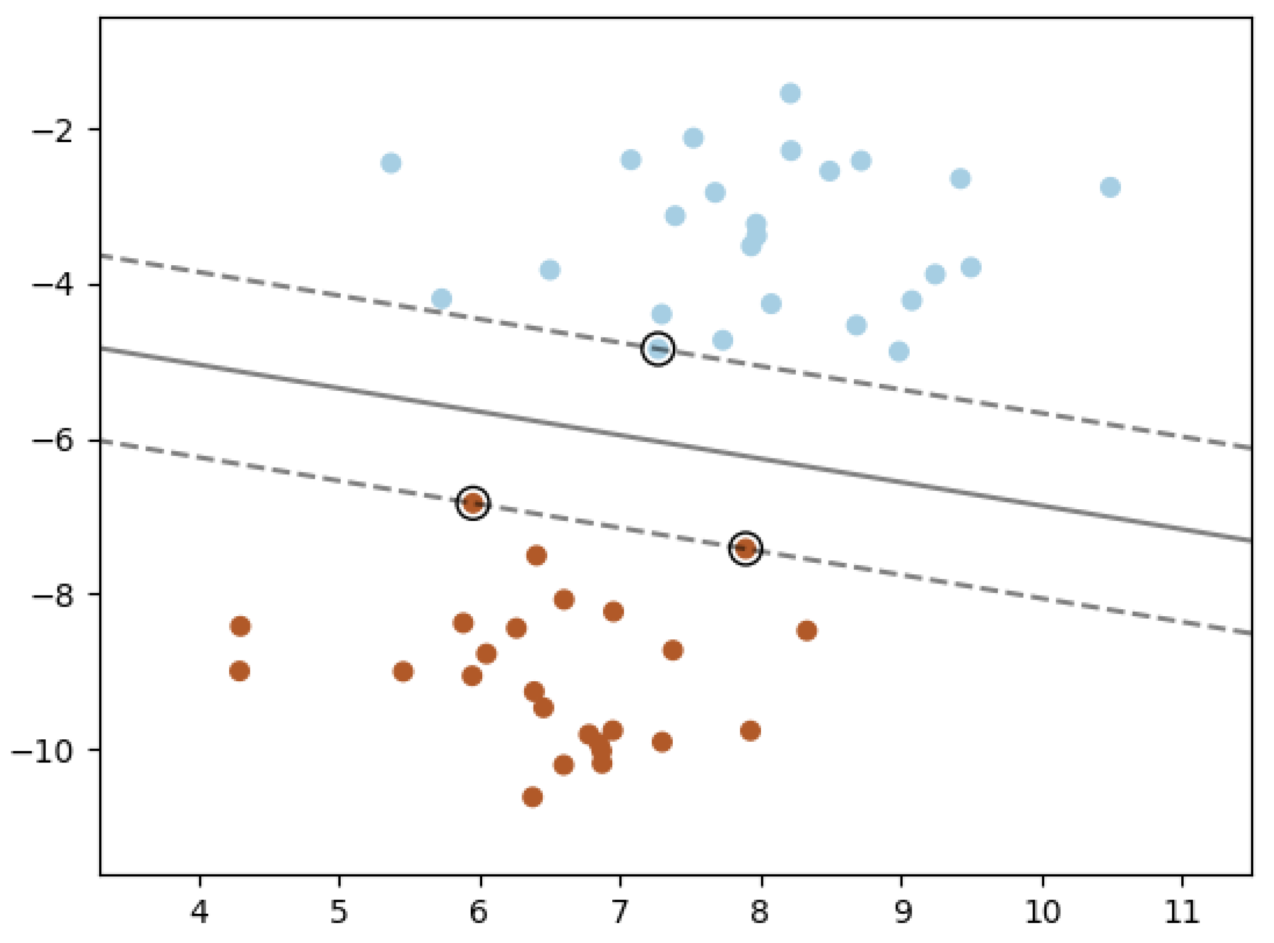
Figure 2.
Representation of the high-level workflow for a quantum variational algorithm.
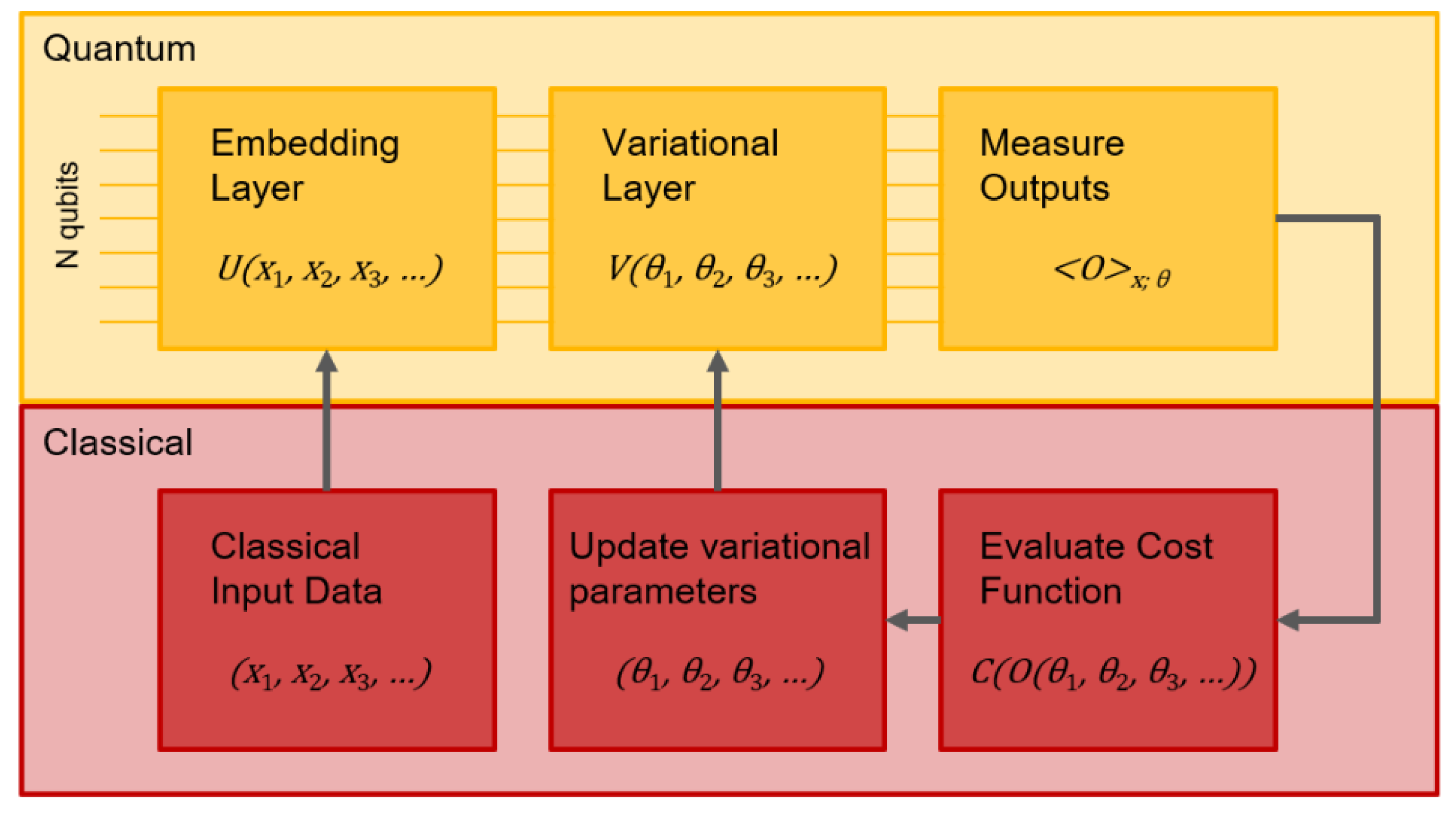
Figure 3.
PRISMA flow diagram of sources selection process.
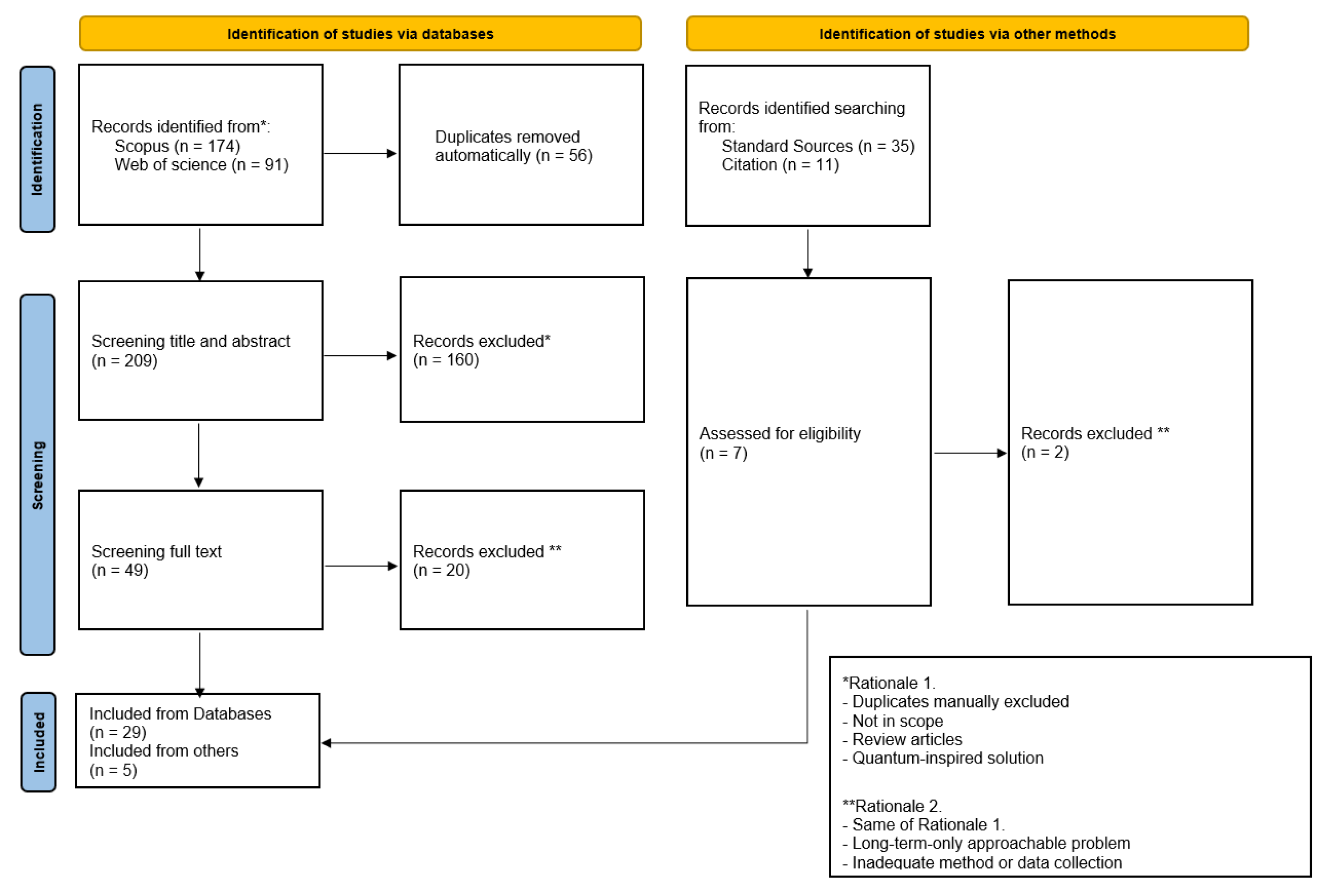
Figure 4.
Distribution of papers and use Cases per value chain.
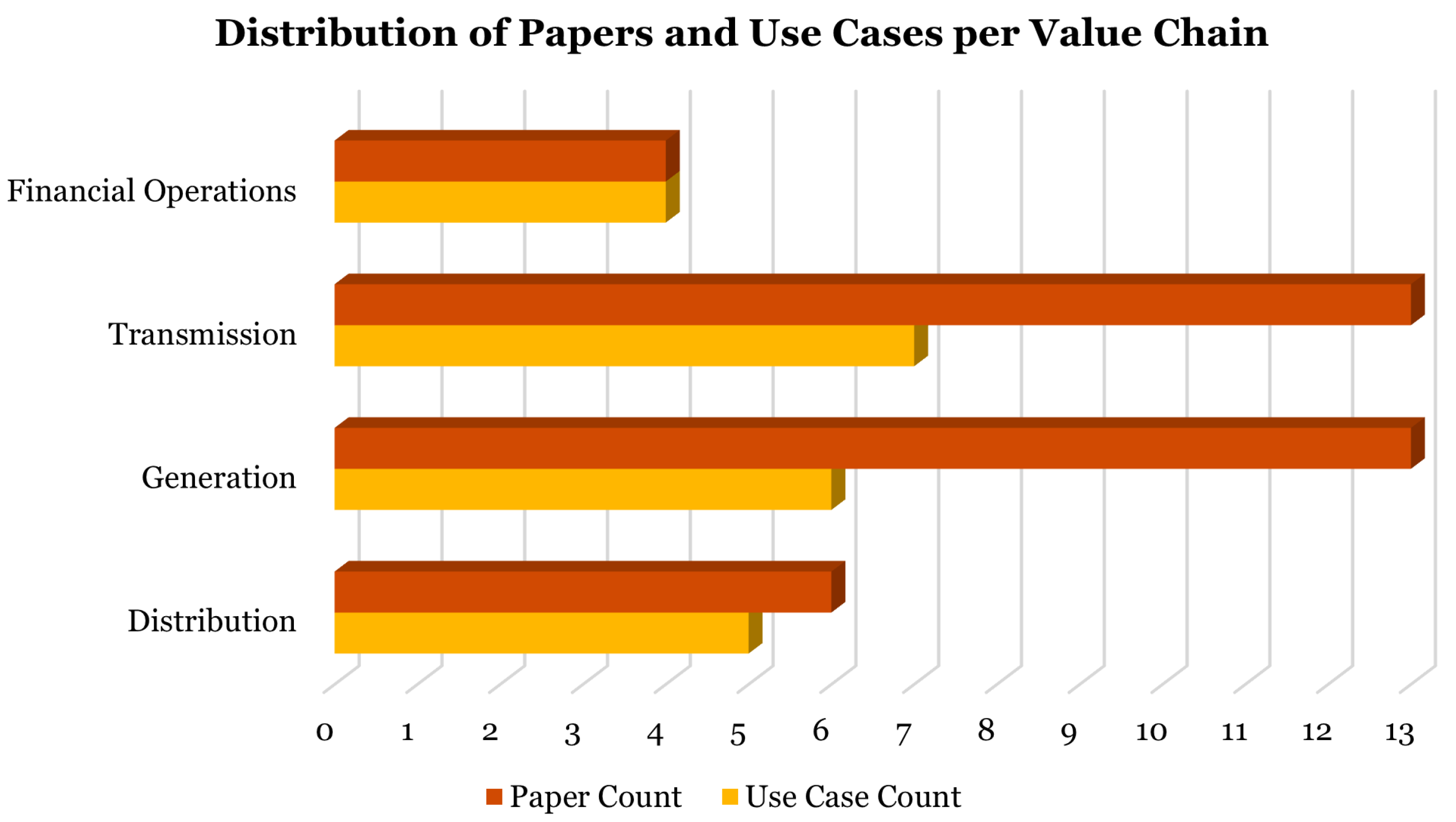
Figure 5.
Distribution of papers per QML typology, type of software and type of hardware employed.
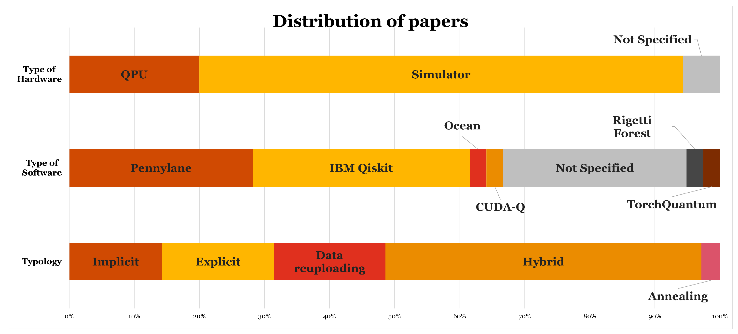
Figure 6.
Impact of quantum computing technology on Predicted Temporal evolution of Offer-demand computational power curves.Once the Full Advantage is virtually reached (TP), Demand is expected to be greater than Offer. And even more so once Supremacy is achieved, Demand grows further. The portion of Demand that cannot be delivered due to Offer limits will remain on hold until the Offer curve reaches that corresponding level of capacity. The length of that time will be likely to dilate as technologies improve, causing companies that are not ready and waiting to lose important competitive advantage. As indicated by the red arrow, Supremacy is getting closer: several shreds of evidence suggest that technology is rapidly accelerating in various directions, and this moment is receding further and further behind with each detection.
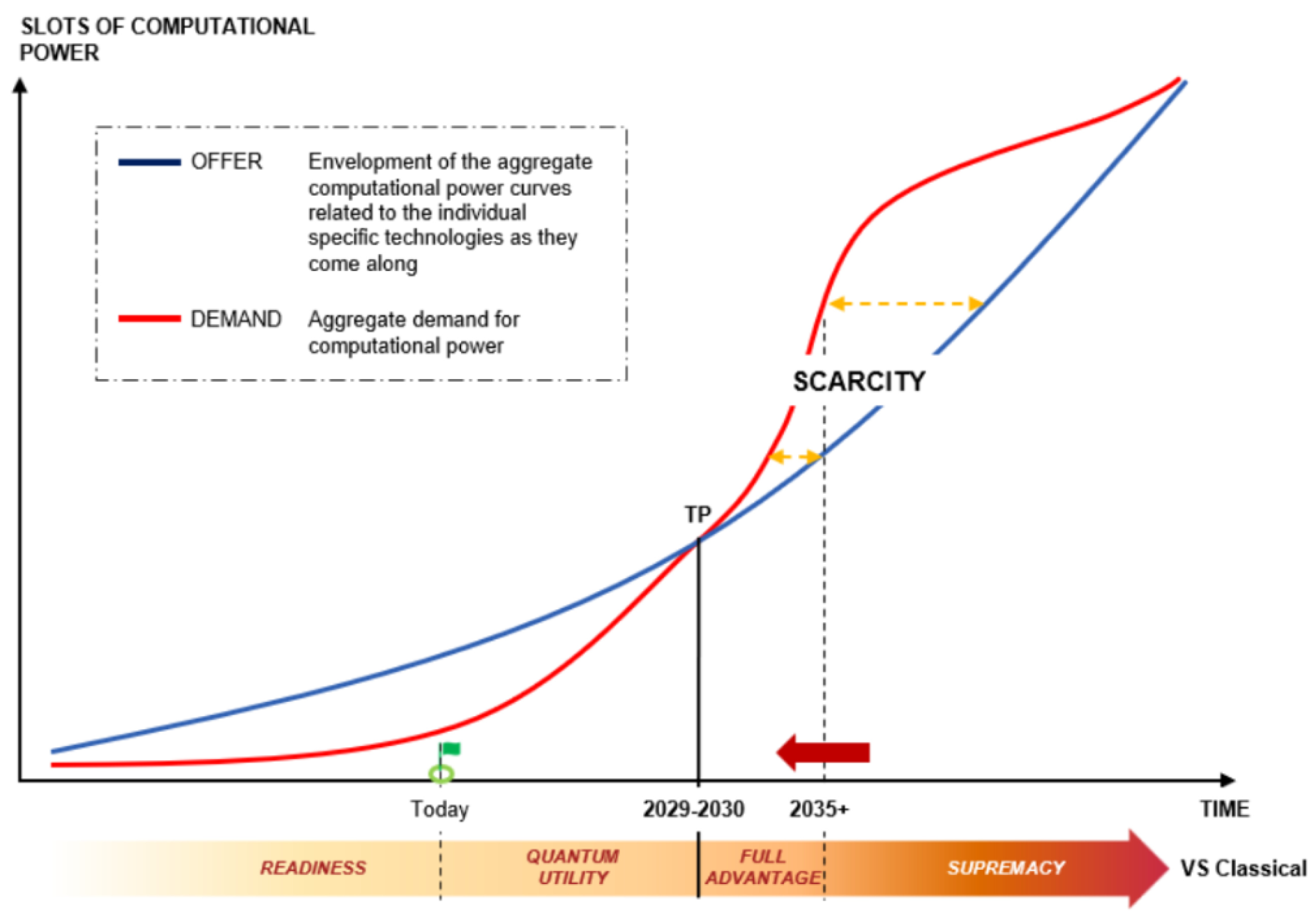
Figure 7.
Graphical Representation of AMIM. (For use case ID mapping see Table 1).
Figure 7.
Graphical Representation of AMIM. (For use case ID mapping see Table 1).
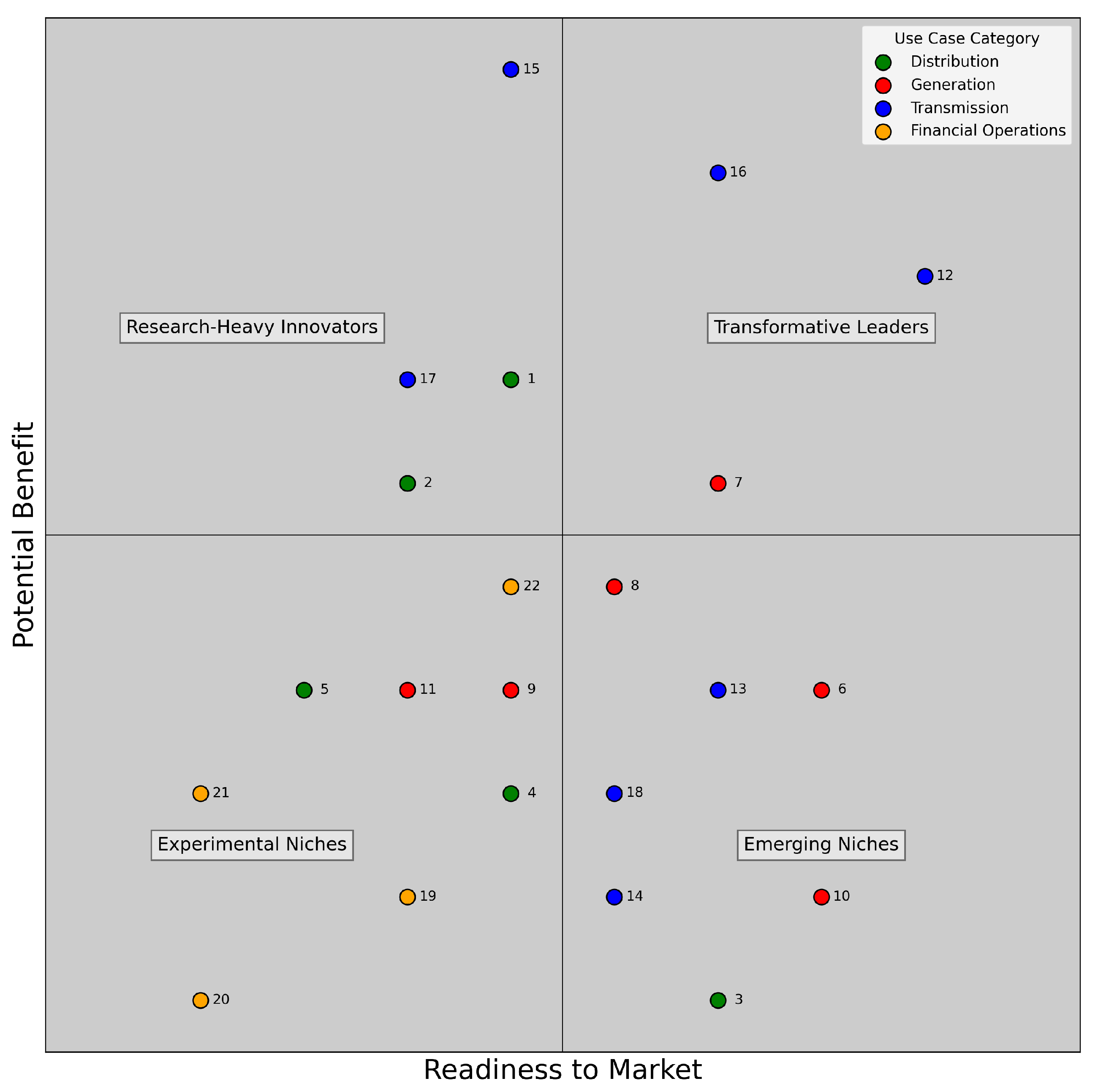

Table 1.
Look-Up Table for Use Cases.
| Value Chain | Category | Use Case | Reference | ID |
|---|---|---|---|---|
| Distribution | Demand Response Systems | Load Forecasting for Demand Response | [67,68] | 1 |
| Automated Demand Response in Smart Cities | [69] | 2 | ||
| Smart Grid Management | HVAC Automated Control in Buildings | [70] | 3 | |
| Appliance Load Signature Identification | [71] | 4 | ||
| Electricity Theft Detection | [72] | 5 | ||
| Generation | Indirect Generation Forecasting | Solar Irradiation Forecasting | [73,74,75,76,77] | 6 |
| Wind Speed Forecasting | [78] | 7 | ||
| Weather and Climate Modeling | [79,80] | 8 | ||
| Direct Generation Forecasting | Photovoltaic Power Forecasting | [81,82,83] | 9 | |
| Forecasting Power from Offshore Wind Farms | [84] | 10 | ||
| Plant Operations | PV Array Topology Optimization | [85] | 11 | |
| Transmission | Maintenance | Fault Diagnosis in Electrical Power Systems | [86] | 12 |
| Photovoltaic Panels Fault Detection | [87] | 13 | ||
| Wind Turbine Pitch Fault Detection | [88] | 14 | ||
| Defect Detection in Wind Turbine Gearbox | [89] | 15 | ||
| Grid Operations | Power System Stability Assessment | [90,91,92,93,94] | 16 | |
| Power Disturbances and Events Identification | [95,96] | 17 | ||
| Smart Grid Stability Forecasting | [97] | 18 | ||
| Financial Operations |
Finance for Sustainable Energy | Carbon Price Forecasting | [98] | 19 |
| Carbon Market Risk Estimation | [99] | 20 | ||
| Blockchain-based P2P Energy Trading for E-Mobility | [100] | 21 | ||
| Smart Energy Distribution | Optimal Scheduling of EV Recharges | [70] | 22 |
Table 2.
Use Case Method’s Overview.
| ID | Method | Typology | SW Technology | HW Technology | Reported Benchmark |
|---|---|---|---|---|---|
| 1 | QSVM | Implicit | Not Specified | Not Specified | RNN, LSTM |
| QNN | Data re-uploading | PennyLane, IBM Quantum Lab | IBM (various devices) | ARIMA, SARIMA, RNN, LSTM, GRU, Ensemble Learning | |
| 2 | Hybrid RL | Hybrid | IBM Qiskit | IBM Brisbane | MPC, DDPG, Lo-DDPG |
| 3 | Hybrid RL | Hybrid | Not Specified | Simulator | NN |
| 4 | VQC | Explicit | IBM Qiskit | Simulator | CNN |
| 5 | VQC | Explicit | IBM Qiskit | Simulator | None |
| 6 | QSVM | Explicit | Not Specified | Simulator | None |
| QLSTM | Hybrid | PennyLane | Simulator | SARIMA, CNN, RNN, GRU, LSTM | |
| QNN | Data re-uploading | IBM Qiskit | Simulator | SVR, XGBoost, GMDH | |
| Hybrid CNN | Hybrid | PennyLane, Torchquantum, CUDA Quantum | Simulator | CNN | |
| Hybrid QNN | Hybrid | PennyLane | Simulator | RNN, LSTM | |
| 7 | QLSTM | Hybrid | PennyLane | Simulator | RF, SVR, XGBoost, NAR, LSTM, LSTM AE |
| 8 | QK-LSTM | Implicit | Not Specified | Simulator | LSTM |
| Physics Informed QNN | Data re-uploading | Not Specified | Not Specified | Spectral Element Method | |
| 9 | QNN, QLSTM, QSeq2Seq | Hybrid | PennyLane | Simulator | RNN, LSTM |
| QLSTM | Hybrid | PennyLane | Simulator | LSTM | |
| VAE-GWO-VQC-GRU | Hybrid | Not Specified | Simulator | GRU | |
| 10 | Hybrid QNN-SVR | Hybrid | PennyLane | Simulator | None |
| 11 | Hybrid QNN | Hybrid | PennyLane | Simulator | NN |
| 12 | Quantum Sampling for CRBM | Annealing | Ocean (D-Wave SDK) | DWave 2000 QPU | NN, DT |
| 13 | QNN | Hybrid | IBM Qiskit | Simulator | NN |
| 14 | QSVM | Implicit | Not Specified | Simulator | RF, k-NN, L-SVM, RBF-SVM |
| 15 | Hybrid CNN | Explicit | IBM Qiskit | Simulator | H-CNN versions |
| 16 | QNN | Data re-uploading | IBM Qiskit | Simulator, ibmq_boeblingen QPU | None |
| QEK with VQC | Implicit | IBM Qiskit | Simulator | Classical kernel methods | |
| QaTSA with ReHELD VQC | Explicit | Not Specified | Simulator | None | |
| QFL with HELD QNNs | Data re-uploading | IBM Qiskit, PennyLane | Simulator, IBM ibm_lagos (7-qubit QPU) | NN | |
| QPCA + VQA | Hybrid | Not Specified | Simulator | PCA | |
| 17 | QVR | Explicit | IBM Qiskit | IBM Falcon r5.11H QPU | LSTM |
| QSVM | Implicit | IBM Qiskit | Simulator | SVM, other classical PQD methods | |
| 18 | VQC | Explicit | Not Specified | Simulator | SVM |
| 19 | QLSTM | Hybrid | PennyLane | Simulator | QLSTM versions |
| 20 | QCGAN + QAE | Data re-uploading | IBM Qiskit | Simulator, IBM QPU | Historical simulation, CGAN, QCGAN |
| 21 | Hybrid RL | Hybrid | Rigetti Forest (PyQuil) | Simulator | Deep Q-Learning |
| 22 | Hybrid RL | Hybrid | Not Specified | Simulator | NN-based RL |
Table 3.
Assessment Model for Innovation Management
| ID | Scalability | Market Compatibility | Implementation Feasibility | Total Readiness to Market | Impact on Efficiency | Criticality of the Problem | Margin for Further Improvement | Total Potential Benefit |
|---|---|---|---|---|---|---|---|---|
| 1 | 4 | 2 | 1 | 7 | 3 | 3 | 3 | 9 |
| 2 | 3 | 1 | 2 | 6 | 4 | 3 | 1 | 8 |
| 3 | 4 | 3 | 2 | 9 | 1 | 1 | 1 | 3 |
| 4 | 4 | 2 | 1 | 7 | 1 | 1 | 3 | 5 |
| 5 | 3 | 1 | 1 | 5 | 3 | 2 | 1 | 6 |
| 6 | 4 | 4 | 2 | 10 | 1 | 3 | 2 | 6 |
| 7 | 3 | 4 | 2 | 9 | 3 | 3 | 2 | 8 |
| 8 | 4 | 3 | 1 | 8 | 2 | 2 | 3 | 7 |
| 9 | 2 | 3 | 2 | 7 | 2 | 2 | 2 | 6 |
| 10 | 4 | 3 | 3 | 10 | 1 | 1 | 2 | 4 |
| 11 | 2 | 2 | 2 | 6 | 3 | 1 | 2 | 6 |
| 12 | 4 | 4 | 3 | 11 | 3 | 4 | 3 | 10 |
| 13 | 4 | 4 | 1 | 9 | 3 | 1 | 2 | 6 |
| 14 | 2 | 4 | 2 | 8 | 1 | 1 | 2 | 4 |
| 15 | 4 | 2 | 1 | 7 | 4 | 4 | 4 | 12 |
| 16 | 4 | 4 | 1 | 9 | 3 | 4 | 4 | 11 |
| 17 | 3 | 2 | 1 | 6 | 3 | 3 | 3 | 9 |
| 18 | 2 | 3 | 3 | 8 | 1 | 1 | 3 | 5 |
| 19 | 2 | 2 | 2 | 6 | 1 | 1 | 2 | 4 |
| 20 | 1 | 1 | 2 | 4 | 1 | 1 | 1 | 3 |
| 21 | 1 | 2 | 1 | 4 | 2 | 1 | 2 | 5 |
| 22 | 3 | 3 | 1 | 7 | 2 | 2 | 3 | 7 |
Disclaimer/Publisher’s Note: The statements, opinions and data contained in all publications are solely those of the individual author(s) and contributor(s) and not of MDPI and/or the editor(s). MDPI and/or the editor(s) disclaim responsibility for any injury to people or property resulting from any ideas, methods, instructions or products referred to in the content. |
© 2025 by the authors. Licensee MDPI, Basel, Switzerland. This article is an open access article distributed under the terms and conditions of the Creative Commons Attribution (CC BY) license (http://creativecommons.org/licenses/by/4.0/).
Copyright: This open access article is published under a Creative Commons CC BY 4.0 license, which permit the free download, distribution, and reuse, provided that the author and preprint are cited in any reuse.


