
Submitted:
20 April 2025
Posted:
21 April 2025
You are already at the latest version
Abstract
A generalized model of the variable permeability in the transition layer is introduced in this work. This model can handle flows with small Darcy number, and might be of utility in controlling permeability amplifications. A method of solution of the resulting inhomogeneous generalized Airy’s equation is presented together with a computational procedure for the arising generalized Airy’s functions and the generalized Nield-Kuznetsov function of the first kind. A complete solution is then provided for the tri-layer flow problem that involves flow over a porous layer with an embedded transition layer.
Keywords:
Transition Layer
; Generalized Airy’s Equation
; Generalized Nield-Kuznetsov Function
1. Introduction
Driven by a host of well-documented applications in natural and industrial settings, including movement of water, oil and gas in ground layers, lubrication theory, blood flow in biological tissues, and various other industrial applications (cf. Bejan and Nield [1] and the references therein) fluid flow through and over porous layers continues to receive unparalleled attention in the porous media literature. Depending on the porous microstructure of the medium, the presence or absence of macroscopic, solid boundaries on which the no-slip condition is imposed, and the importance of inertial effects in the medium, the flow of an incompressible fluid is governed by the continuity equation
and a general momentum equation which, in the absence of body force, is written in the following form when permeability is constant [2,3]
where is the fluid velocity vector field, is the permeability tensor, is the pressure, is the fluid density, is the base fluid viscosity, is the relative viscosity, is the effective viscosity (viscosity of the fluid in the porous medium), is the convective acceleration parameter, and are binary parameters, and is the Forchheimer drag coefficient.
The parameters take on the values or . By assigning the values or to parameters , the main models of fluid flow through porous media and in free-space are recovered. For instance, if , the flow is in free-space and equation (2) reduces to the Navier-Stokes equations. If , the flow is in the porous medium, and the following flow models (Table 1) are recovered, [3].
Flow over porous layers involves flow through a free-space channel over a porous layer, or flow through a composite of porous layers of different porosities and permeabilities (cf. [4,5,6,7,8] and the references therein). Its direct influence on heat and mass transfer processes in various physical settings mandates accurate modelling of the flow processes and the associated interfacial conditions between flow domains, [9,10,11,12,13,14]. Based on equation (1), uni-directional flow in channels and porous layers is governed by the following equation, wherein is the tangential velocity component:
Equation (3) provides a single-equation for simulation of flow through and over porous layers by simply switching parameters.
Experimental and theoretical studies in the field of flow over porous layers span more than six decades, and include the development of an expansive body of knowledge that initially focused on the use of Darcy’s equation as a model of flow through the porous layer and resulted in the development of Beavers and Joseph slip hypothesis, [15], and the following condition at the interface, , between a free-space layer and the porous layer
where is the Darcy velocity, and is an empirical slip parameter with a range of values 0.1 to 4, (cf. [1,15,16,17].
The Beavers and Joseph condition continues to be addressed by various authors (cf. [1,18,19,20,21] and the references therein). Concerns about the low order of Darcy’s equation and the slip parameter in Beavers and Joseph’s experiments resulted in the development of interfacial conditions centred on velocity and shear stress continuities, and the use of Brinkman’s equation, [22], as a viable alternative to Darcy’s equation. Furthermore, if Darcy’s equation is replaced by another flow model, such as the Forchheimer equation, then the slip parameter needs to be adjusted, as discussed by Roach and Hamdan, [23]. Neale and Nader, [19], provided the following conditions at the assumingly sharp interface between a free-space channel and a Brinkman porous layer (-h<y<0), and identified the slip parameter with :
Brinkman’s equation, [22], continues to receive attention by various authors, whether to discuss its validity or its limitations (cf. [1,18,24,25,26] and the references therein).
It is generally agreed that, in the flow over a porous layer, if the porous layer is of infinite depth, then the flow in the porous layer is governed by Darcy’s equation, while if the porous layer is of finite depth, then Brinkman’s equation should be used (cf. Rudraiah [7] and the references therein).
Ochoa and Whitaker [20,21] developed a stress jump condition at the interface, which takes into account momentum transfer at the interface, and is of the form
where is an adjustable jump parameter. The absence of definite values hinders the efficient use of the Ochoa-Whitaker jump stress condition , hinders its accurate use, [28].
Many of the interfacial conditions and models in use assume the existence of a sharp interface, and do not account for permeability discontinuity at the interface between free-space and the porous layer, or between two porous layers of different permeabilities. Extensive analyses have been carried out to point the need for interfacial modeling that takes into account gradual changes in permeability from its finite value in the porous medium to its approach to infinity in the absence of a porous matrix, or a gradual change in permeability from one finite value to another different finite value in the case of flow through a porous layer underlain by another porous layer, [29].
Recent advancements in the field, however, concluded that permeability continuity is better handled through the introduction of a thin transition region between a homogeneous porous layer and free-space, or between two homogeneous porous layers. The concept of the transition layer has been implemented and validated in the analysis provided by number of authors [9,13,14,18,28,30,31,32,33,34]. The transition layer is characterized by its variable permeability that smoothly changes between its value in the homogeneous porous sediment and infinity in the free-space channel, or between two finite permeability values in two adjacent homogeneous porous layers. The crux of the problem is then narrowed down to modeling flow through a variable permeability porous layer the flow through which is governed by Brinkman’s equation. This has given an impetus to Brinkman’s equation and its usefulness.
It is worth noting that the use of the transition layer is not restricted to flow over a porous layer. Rather, three transition layer scenarios are possible in this type of tri-layer analysis. The first is a transition layer between a Navier-Stokes channel and a constant permeability porous layer of infinite depth. In this case, the flow in the constant permeability layer is governed by Darcy’s law.
The second is a transition layer between the Navier-Stokes channel and a homogeneous porous layer of finite depth. In this case, the flow in the constant permeability finite layer is governed by Brinkman’s equation. The third involves a transition layer inserted between two Darcy layers, or between two homogeneous Brinkman layers, or a combination of both. In all of these cases, the mathematical problem reduces to that of a Poiseuelle-type flow configuration, or a uni-directional flow problem in a tri-layer flow domain.
Many investigations and models exist for flow through variable permeability porous layers, (cf. [35,36,37,38] and the references therein). Roach and Hamdan, [39], provided a review and a classification of the available variable permeability models.
A most suitable model was introduced in the work or Nield and Kuznetsov [30], where the reciprocal of the permeability varies across the transition layer according to , where is the overall tri-layer thickness, is related to the thickness of the transition layer, is the transition layer permeability, and is the constant permeability of the underlying porous layer. This choice of permeability distribution reduces Brinkman’s equation in the transition layer to an Airy’s inhomogeneous ordinary differential equation of the form:
where is the transition layer thickness, is the flow velocity in the transition layer, and is the Darcy number that is defined in terms of a constant reference permeability, . Equation (8) is the well-known Airy’s inhomogeneous equation.
In the process of their solution, Nield and Kuznetsov [30] introduced a new integral function, , to express the particular solution to the resulting Airy’s inhomogeneous equation. The function is referred to in the literature as the Nield-Kuznetsov function, [40], and is defined in terms of Airy’s functions of the first- and second-kind, and , respectively, as
General solution to (8) is thus expressed as:
where The Nield-Kuznetsov function and its role in the transition layer was successfully implemented by Tao et al. [28], who presented elegant and detailed analysis of the effects of the transition layer parameters involved in the modelling process, where they employed two specific permeability functions to express permeability variations. Tao et al. [28] provided details of the amplifications in the transition layer permeability and emphasized the need for an exact description of the permeability in the transition layer and a precise permeability forecasting function to model the gradual change of permeability along the transition layer region to better match the velocity distribution with experimental results.
Tao et al. [28] employed ascending series representations in the evaluations of . Nield and Kuznetsov [30] evaluated then using asymptotic series expansions and reported that the smallest value of they could compute their results for was , and stated that as tends to zero, becomes large and results in singularity. While there is no claim that we know the reason as to why this happened, it is quite possible that the above-mentioned use of asymptotic series (valid for large values of ) as opposed to ascending series (valid for all values of ) played a role. We also point out that in the expression for , the transition layer thickness, , is a positive, finite quantity less than unity, and that is also finite. If we write the coefficient of in equation (8) as , then as , and , the expression becomes excessively large, unless the numerator in the expression approaches zero at the same rate as approaches zero. One possibility is to introduce a permeability model that leads to in the numerator, where is a positive integer. By adjusting the value of , it might be possible to obtain solutions for small values of . In the current work, the smallest value of Darcy number that we could use in computations involving a thin transition layer and the use of was . Furthermore, the suggested choice of permeability function might prove effective in reducing permeability amplifications in the transition layer that Tao et al. [28] discussed.
This observation, together with the success attained by Nield and Kuznetsov, [30], and Tao et al. [28], in advancing the state of knowledge of flow in the transition layer, motivates the introduction of other integral functions to model variations of permeability in the transition layer. In fact, in a recent study where a porous layer was embedded between two fluid layers, Abu Zaytoon and Hamdan, [41], employed a permeability function that reduced Brinkman’s equation to Weber’s inhomogeneous equation, the solution to which they obtained in terms of the parametric Nield-Kuznetsov function.
In the current work, we introduce a generalized permeability function, to describe the variable permeability in the transition layer, that offers modeling flexibility and can be reduced to the permeability function used by Nield and Kuznetsov [30]. Brinkman’s equation governing flow in the transition layer can then be reduced to a generalized Airy’s equation (in the sense introduced by Swanson and Headley [42]). An efficient evaluation procedure of the special functions that arise in the solution of the resulting governing equation is presented, and solutions are obtained for a choice of flow parameters. The solution provided by Nield and Kuznetsov [30] is then compared with a special case of the current formulation, which shows agreement between solutions obtained. It is believed that the current approach will provide extended flexibility in modelling permeability variations in the transition zone.
2. Problem Formulation
Consider the flow of an incompressible fluid in the tri-layer model of Figure 1, below, in which layer 1 represents a free-space channel the flow through which is governed by Navier-Stokes equations. Layer 3 is a homogeneous porous layer of constant permeability, the flow through which is governed by Brinkman’s equation. Layer 2 is the transition layer the flow through which is governed by Brinkman’s equation with variable permeability. The flow in the configuration is driven by a common pressure gradient.
Permeability distribution is given as follows, where we take as a constant reference permeability, and assume that flow in the free-space layer 1 has an infinite conductivity to the fluid.
Equations governing the flow in the respective regions are given by:
In the above equations, is the constant pressure gradient, the quantities and represent the velocity and permeability in region , for respectively; is the base fluid viscosity and , are the effective viscosities, respectively, in regions 2 and 3.
We point out here that in the above formulation, we interchanged layers 1 and 3 in the original formulation by Nield and Kuznetsov, [30]. However, for the sake of comparing results, we solve the flow equations in both configurations.
Following Nield and Kuzentsov [30], we introduce the following dimensionless variables, where refers to Darcy number; ; for ; and for , to transform governing equations (14)-1(6), respectively, into:
where
The dimensionless permeability distributions, , can be written in the following dimensionless form in terms of Darcy number, :
Equations (17), (18) and (19) must be solved subject to the following boundary and matching conditions
We note that if , then corresponds to that was used in the work of Nield and Kuznetsov [30]. General solutions for equation (17) and (19) are given, respectively, by
Upon using the transformation and writing , equation (18) can be written as:
Equation (27) is recognized as the generalized inhomogeneous Airy’s differential equation, Swanson and Headley [42]. A fundamental set of linearly independent solutions for the homogeneous part of (27) are the generalized Airy’s functions and , defined respectively by, [42]:
The Wronskian of and is given by:
and the terms are the modified Bessel functions defined as:
with , , , and is the gamma function. Solution to the homogeneous part of (27) thus takes the form
A particular solution to equation (27) is expressed in the form
wherein
U2𝑝y = σnNn(y)
The function , defined in (36), is known as the Generalized Nield-Kuznetsov Function of the First Kind, [34]. When , equation (27) reduces to Airy’s equation and (36) reduces to the Standard Nield-Kuznetsov Function of the First Kind, , defined by Nield and Kuznetsov in [30].
General solution to equation (27) thus takes the form
Upon using and , general solution (37) is expressed as:
Derivatives of the functions , and are given by:
Upon using boundary and interfacial conditions, (22)-(24), the constants in equations (25), (26) and (38), satisfy the following system of linear equations, written in the form , where:
In solving the above linear system, we take and make use of the following values of the generalized functions , and , and their first derivatives at zero, namely:
Following Swanson and Headley, [42], the generalized Airy’s functions are evaluated using the following relationships:
and the Generalized Nield-Kuznetsov Function of the First Kind can be evaluated using the following expression:
3. Results and Discussion
Results have been obtained for a range of values of n and the range of Da = 1; 0.1; 0.001; 0.0001; 0.00001; and 0.000001 in order to illustrate the effects of changing n and Da on the generalized functions, on the permeability function, on the arbitrary constants, and on the velocity profiles. Thick and thin transition layers are considered. In particular, we choose , for thick transition layer and , for thin transition layer.
3.1. Permeability Distributions
Dimensionless permeability distribution in the transition layer is given by equation (12), namely , and its dependence on the values of n, Da, and the thickness of the porous layer are illustrated in Figure 2, Figure 3 and Figure 4, for the thick and thin transition layer, respectively, Da = 1, and various values of n. These figures demonstrate how n acts as a control parameter in the permeability distribution. Figure 4 shows the effect of Da on the permeability distribution for n = 1 and thin transition layer. The graph is zoomed in to better illustrate the distribution when Da = 0.000001.
3.2. Velocity Profiles
Figure 5 illustrates the velocity profiles across the three layer flow configuration for the case of thin transition layer, n =1, and various values of Da. The transition layer thickness is shown on the graphs as a small thick line (smudge) on each graph.
In using the solution procedure given by equations (44)-(49), the smallest Darcy number we could compute results for was However, results are shown for a smallest value of , when . Figure 5 shows smooth transitions from one flow domain layer to another for the range of used. As Da increases, the singularity at the lower interface starts creeping in (as anticipated by Nield and Kuznetsov [ ]). When n=2, Figure 6 illustrates a similar pattern of velocity profiles, and shows a more noticeable effect of the singularity at the lower interface. This emphasizes that the current model and solution procedure is more suitable for low values of Da.
For different values of n, and a fixed value of Da, the velocity profiles are close to each other (due to graph scale) and follow a similar pattern and shape to the profiles of Figure 6. Therefore, to better demonstrate the relative magnitudes of velocities for various values of n, velocity profiles are sketched over the span of the thin transition layer , illustrated in Figure 7. The increase in permeability in the transition layer with increasing n is accompanied with an increase in velocity, as Figure 7 demonstrates.
3.3. Velocity at the Interfaces
At the lower and upper interfaces, and , respectively, velocity expressions are obtained from equations (25), (26), and (38), and take the form
Velocity at the lower and upper interfaces for thick and thin transition layers, for different values of Da and different values of n, are given in Table 2 and Table 3. In Table 2, velocity at the upper interface is illustrated for the thick transition layer, only, since the behaviour is similar for the thin layer, for n=1,2,3 and various values of Da.
As n increases, for a fixed value of Da, interfacial velocity increases since permeability increases as we get closer to the upper interface. This behaviour is consistent for all values of Da shown. Interfacial velocity consistently increases with increasing Da for any fixed value of n, as expected.
In Table 3, velocity at the lower interface is illustrated for the thin transition layer, only, since the behaviour is similar for the thick layer, for n=1,2,3 and various values of Da.
As n increases, for a fixed value of Da, interfacial velocity decreases. This is due to the velocity continuity condition at the lower interface where the velocity in the homogeneous, constant permeability layer has the effect of slowing down the flow velocity at the interface.
This behaviour is consistent for all values of Da shown. Interfacial velocity consistently increases with increasing Da for any fixed value of n, since Da is defined in terms of a fixed, reference permeability.
Agreement between the values computed using equations (50) and (51) was for more than 12 significant digits, which indicates that the current formulation and computations are accurate. Similarly when using equations (52) and (53). In Table 2 and Table 3 we retained the first 8 digits for illustration.
3.4. Shear Stress at the Interfaces
At the lower and upper interfaces, and , respectively, shear stress expressions are obtained from equations (25), (26), and (38), and take the form
Shear stress values at the lower and upper interfaces for different middle layer thickness, and for n = 1, 2, 3, are given in Table 4, which furnish the following observations.
- For a given Da, the value of the shear stress at the upper interface decreases with increasing n for the thick layer. However, it increases with increasing n for thin layer.
- For a given Da, the value of the shear stress at the upper interface increases with increasing n for the thin layer, and decreases with increasing n for the thick layer.
- The thin layer experiences a higher sheer than the thick layer at the upper interface with increasing n.
- The thick layer experiences a higher sheer than the thin layer at the lower interface when n deviates from 1.
3.5. Mean Velocity Across the Layers
The dimensionless mean velocities across the lower and upper layers are defined, respectively, as
Dimensionless mean velocity in the transition layer is obtained from (38) and can be written as:
where .
The dimensionless mean velocity across the configuration (that is, across the three layers) is defined as
and represents a measure of the overall volume flux through the channel configuration.
The above expressions are evaluated using Maple and the values are listed in for n = 1 and n = 2 in Table 5 for different transition layer thicknesses and Da = 1, 0.1, and 0.01 so that we can compare our results with those obtained by Nield and Kuznetsov [30]. To make the comparison, we reformulated and solved the flow problem using the same configuration as that of Nield and Kuznetsov [30]. Agreement between the results is evident from Table 5.
For a given transition layer thickness and a given value of n, the total volume flux decreases with decreasing Da. This is due to flow retardation for smaller Da. For a given Da, the total volume flux increases with increasing n.
4. Conclusions
In this work, we considered the problem of flow through a free-space channel over a porous layer in the presence of a transition porous layer. This problem was treated by Nield and Kuznetsov [30] to illustrate the characteristics of the flow when the transition layer is a Brinkman layer of variable permeability described as the reciprocal of a linear polynomial. In this work we introduced a generalized form of the permeability function that involves the reciprocal of the nth degree of the a linear polynomial. This choice of permeability function resulted in the inhomogeneous, generalized Airy’s differential equation. We provided the solution to the resulting differential equation in terms of a generalized Nield-Kuznetsov function, together with a computational procedure to evaluate the arising special functions. For the case of n = 1, the current problem reduces to the one considered by Nield and Kuznetsov, [30], and our results agree with their results for total volume flux across the tri-layer configuration.
Highlights of this work may be stated as follows:
- The introduction of a generalized permeability function that provides modeling flexibility and validity for small Darcy number, and possible control over permeability amplification in the transition layer.
- Obtaining the general and particular solutions to the resulting inhomogeneous generalized Airy’s equation through the introduction of a generalized Nield-Kuznetsov function.
- Providing an evaluation procedure for the arising generalised Airy’s functions and the generalized Nield-Kuznetsov function.
Author Contributions
Authors contributed equally to this research. Conceptualization, M.H. and M.S.; methodology, M.H. and M.S.; software, M.S.; validation, M.H. and M.S.; formal analysis, M.H. and M.S.; investigation, M.H. and M.S.; resources, M.H.; data curation, M.S.; writing—original draft preparation, M.H.; writing—review and editing, M.S.; project administration, M.H. All authors have read and agreed to the published version of the manuscript.”
Funding
This research received no external funding
Data Availability Statement
All data was created using MAPLE and is included in this work.
Conflicts of Interest
The authors declare no conflicts of interest.
References
- Nield, D.A.; Bejan, A. Convection in porous media, 5th ed.; Springer: New York, 2017.
- Hamdan, M.H. Single-phase flow through porous channels: a review. Flow models and channel entry conditions. J. Applied Math. Comp. 1994, 62, 203-222. [CrossRef]
- Ford, R.A.; Abu Zaytoon, M.S.; Hamdan, M.H. Simulation of flow through layered porous media. IOSR J. Eng. 2016, 6, 48-61.
- Alazmi, B.; Vafai, K. Analysis of fluid flow and heat transfer interfacial conditions between a porous medium and a fluid layer. Int. J. of Heat Mass Transfer. 2001, 44, 1735-1749. [CrossRef]
- Vafai, K.; Thiyagaraja, R. Analysis of flow and heat transfer at the interface region of a porous medium. Int. J. Heat Mass Transfer. 1987, 30, 1391-1405. [CrossRef]
- Kaviany, M. Laminar flow through a porous channel bounded by isothermal parallel plates. Int. J. Heat Mass Transfer.1985, 28, 851-858. [CrossRef]
- Rudraiah, N. Coupled parallel flows in a channel and a bounding porous medium of finite thickness, J. Fluids Eng. ASME. 1985, 107, 322-329.
- Rudraiah, N. Flow past porous layers and their stability. Encyclopedia of Fluid Mechanics, Slurry Flow Technology, Gulf Publishing, 1986, pp. 567-647.
- Hill, A. A.; Straughan, B. Poiseuille flow in a fluid overlying a porous medium. J. Fluid Mech. 2008, 603, 137-149.
- Goyeau, B.; Lhuillier, D.; Velarde, M. G. Momentum transport at a fluid-porous interface. Int. J. Heat Mass Transfer. 2003, 46, 4071-4081.
- Kaviany, M. Laminar Flow through a porous channel Bounded by isothermal parallel plates, Int. J. Heat Mass Transfer 1985, 28, 851-858.
- Sahraoui, M.; Kaviany, M. Slip and no-slip velocity boundary conditions at interface of porous, plain media. Int. J. Heat Mass Transfer. 1992, 35, 927-943. [CrossRef]
- Jamet, D.; Chandesris, M. Boundary conditions at a planar fluid-porous interface for a Poiseuille flow. Int. J. Heat Mass Transfer 2006, 49, 2137-2150.
- Jamet, D.; Chandesris, M. Boundary conditions at a fluid-porous interface: An a priori estimation of the stress jump coefficients. Int. J. Heat Mass Transfer 2007, 50, 3422-3436.
- Beavers, G.S.; Joseph, D.D. Boundary conditions at a naturally permeable wall. J. Fluid Mech. 1967, 30, 197-207.
- Nield, D.A. The Beavers–Joseph boundary condition and related matters: A historical and critical note. Transp Porous Med. 2009, 78, 537–540.
- Ehrhardt, M. An Introduction to Fluid-Porous Interface Coupling. Weierstrass Institute for Applied Analysis and Stochastics, Berlin, 2010.
- Parvazinia, M.; Nassehi, V.; Wakeman, R. J.; Ghoreishy, M. H. R. Finite element modelling of flow through a porous medium between two parallel plates using the Brinkman equation. Transp. Porous Med. 2006, 63, 71-90.
- Neale, G.; Nader, W. Practical significance of Brinkman’s extension of Darcy’s law: coupled parallel flows within a channel and a bounding porous medium. Canadian J. Chem. Eng. 1974, 52, 475-478.
- Ochoa-Tapia, J. A.;Whitaker, S. Momentum transfer at the boundary between a porous medium and a homogeneous fluid: I) Theoretical Development. Int.J. Heat Mass Transfer 1995, 3, 2635-2646. [CrossRef]
- Ochoa-Tapia, J. A.;Whitaker, S. Momentum transfer at the boundary between a porous medium and a homogeneous fluid: II) Comparison with experiment. Int. J. Heat Mass Transfer 1995, 3, 2647-2655.
- Brinkman, H.C. A Calculation of the viscous force exerted by a flowing fluid on a dense swarm of particles. Appl. Sci. Res. 1947, A1, 27-34.
- Roach, D.C.; Hamdan, M.H. Interfacial velocities, slip Parameters and other theoretical expressions arising in the Beavers and Joseph condition. WSEAS Transactions on Fluid Mechanics 2022, 17, 68-78.
- Nield, D.A. The boundary correction for the Rayleigh-Darcy problem: limitations of the Brinkman equation. J. Fluid Mech. 1983, 128, 37-46. [CrossRef]
- Nield, D.A. The limitations of the Brinkman- Forchheimer equation in modeling flow in a saturated porous medium and at an interface. Int. J. Heat Fluid Flow 1991, 12, 269-272.
- Auriault, J.L. On the domain of validity of Brinkman’s equation. Transp. Porous Med. 2009, 79, 215–223.
- Haider, F.; Hayat, T.; Alsaedi, A. Flow of hybrid nanofluid through Darcy-Forchheimer porous space with variable characteristics. Alexandria Eng. J. 2021, 60, 3047-3056. [CrossRef]
- Tao, J.; Yao, J.; Huang, Z. Analysis of the laminar ow in a transition layer with variable permeability between a free-fluid and a porous medium. Acta Mech. 2013, 224, 1943-1955.
- Abu Zaytoon, M. S.; Alderson, T. L.; Hamdan, M. H. Flow through variable permeability composite porous layers. Gen. Math. Notes. 2016, 33, 26-39.
- Nield, D.A.; Kuznetsov, A.V. The effect of a transition layer between a fluid and a porous medium: shear flow in a channel”, Transp. Porous Med. 2009, 78, 477-487.
- Goharzadeh, A.; Khalili, A.; Jorgensen, B. B. Transition layer thickness at a fluid-porous interface. Phys. Fluids. 2005, 17, 1057102-10571021.
- Duman , T.; Shavit, U. A solution of the laminar ow for a gradual transition between porous and fluid domains. Water Res. Research 2010, 46, 09517.
- Abu Zaytoon, M. S.; Alderson, T. L.; Hamdan, M. H. Flow through layered media with embedded transition porous layer. Int. J. of Enhanced Res. In Sci., Tech. and Eng. 2016, 5, 9-26.
- Abu Zaytoon, M. S.; Alderson, T. L.; Hamdan, M. H. Flow through a variable permeability Brinkman porous core. J. Appl. Math. Phys. 2016, 4, 766– 778. [CrossRef]
- Hamdan, M.H.; Kamel, M.T. Flow through variable permeability porous layers. Adv. Theor. Appl. Mech. 2011, 4, 135-145.
- Rees, D.A.S.; Pop, I. Vertical free convection in a porous medium with variable permeability effects. In. J. Heat Mass Transfer 2000, 43, 2565-2571. [CrossRef]
- Siginer, D.A.; Bakhtiyarov, S. I. Flow in porous media of variable permeability and novel effects. J. Appl. Mech. 2001, 68, 312-319. [CrossRef]
- Vafai, K. Analysis of the channeling effect in variable porosity media, ASME J. Energy Resources and Technology 1986, 108, 131–139. [CrossRef]
- Roach, D.C.; Hamdan, M.H. Variable permeability and transition layer models for Brinkman equation. In Proceedings Int. Khazar Sci. Res. Conference-III, Khazar University, Baku, Azerbaijan, January 7-9, 2022, IKSAD Publishing House ISBN: 978-625-8423-84-6, pp. 184-191.
- Hamdan, M.H.; Kamel, M.T. On the Ni(x) integral function and its application to the Airy’s non homogeneous equation. Appl. Math. Comput. 2011, 21, 7349-7360. [CrossRef]
- Abu Zaytoon, M.S.; Hamdan, M.H.: Weber equation model of flow through a variable permeability porous core bounded by fluid layers. J. Fluids Eng., Trans. ASME, 2022, 144, 041302. [CrossRef]
- Swanson, C. A.; Headley, V. B. An extension of Airy’s equation. SIAM J. Appl. Math. 1967, 15, 1400-1412. [CrossRef]
Figure 1.
Representative Sketch of a Tri-layer Channel.
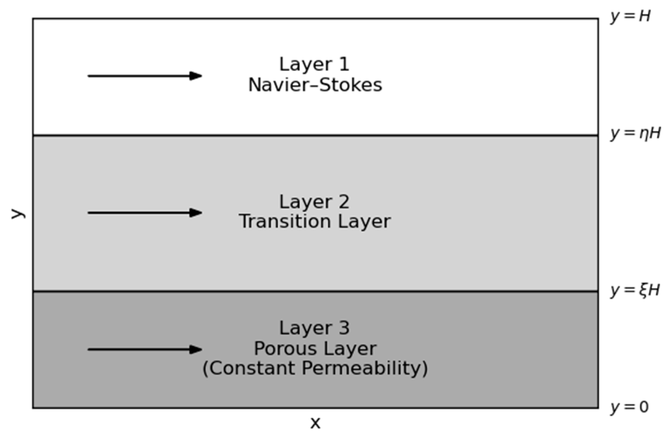
Figure 2.
Dimensionless Permeability Distribution. Thick Layer; Da=1; n=1,2,3,4,5
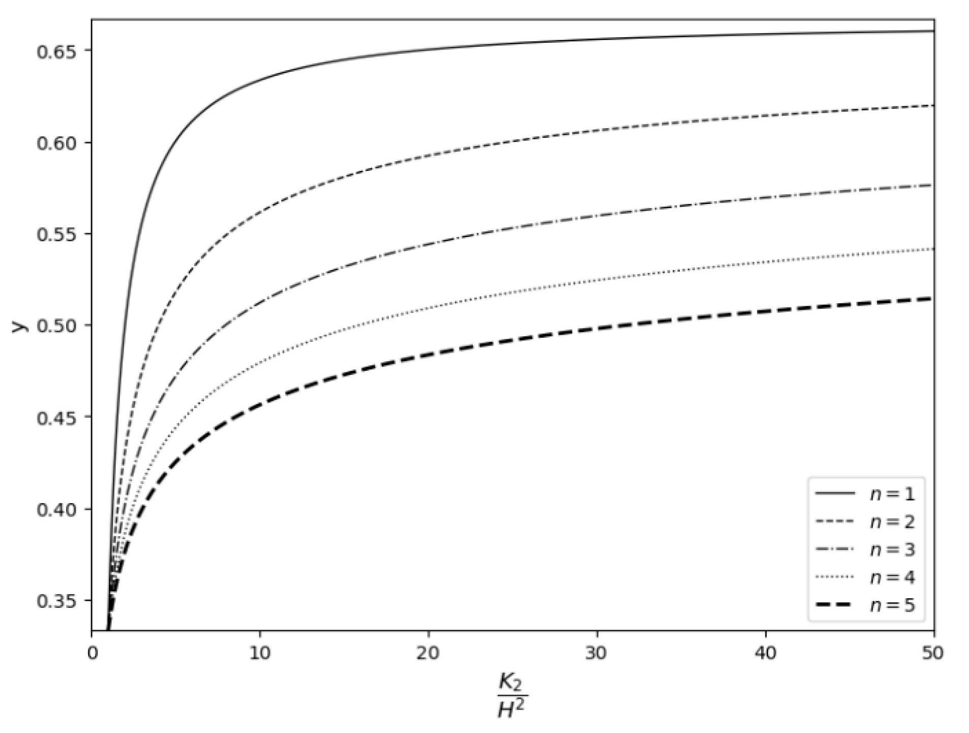
Figure 3.
Dimensionless Permeability Distribution. Thin Layer; Da=1; n=1,2,3,4,5
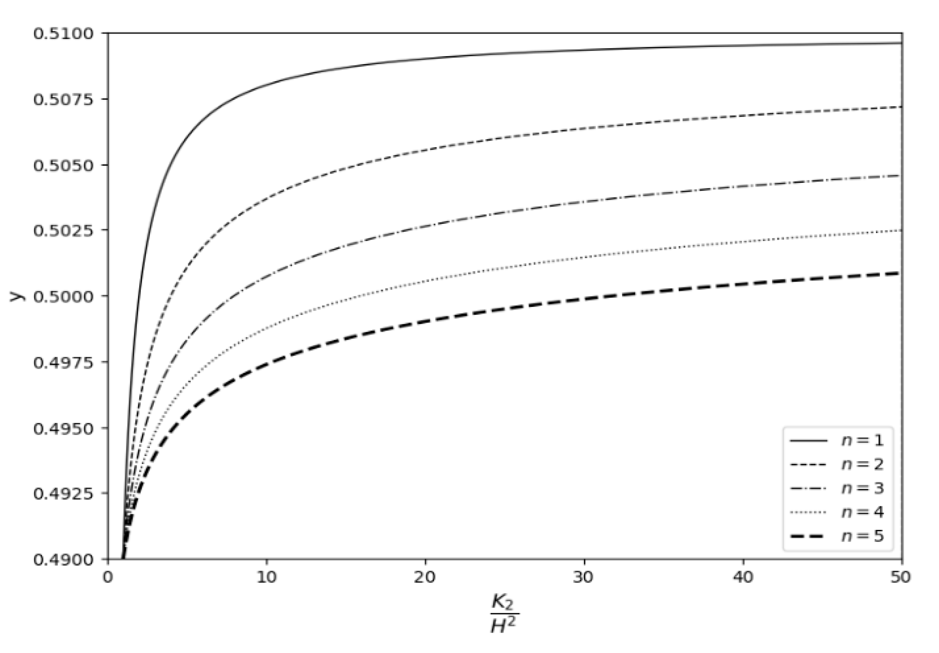
Figure 4.
Dimensionless Permeability Distribution. Thin Layer; n=1; Various Values of Da.
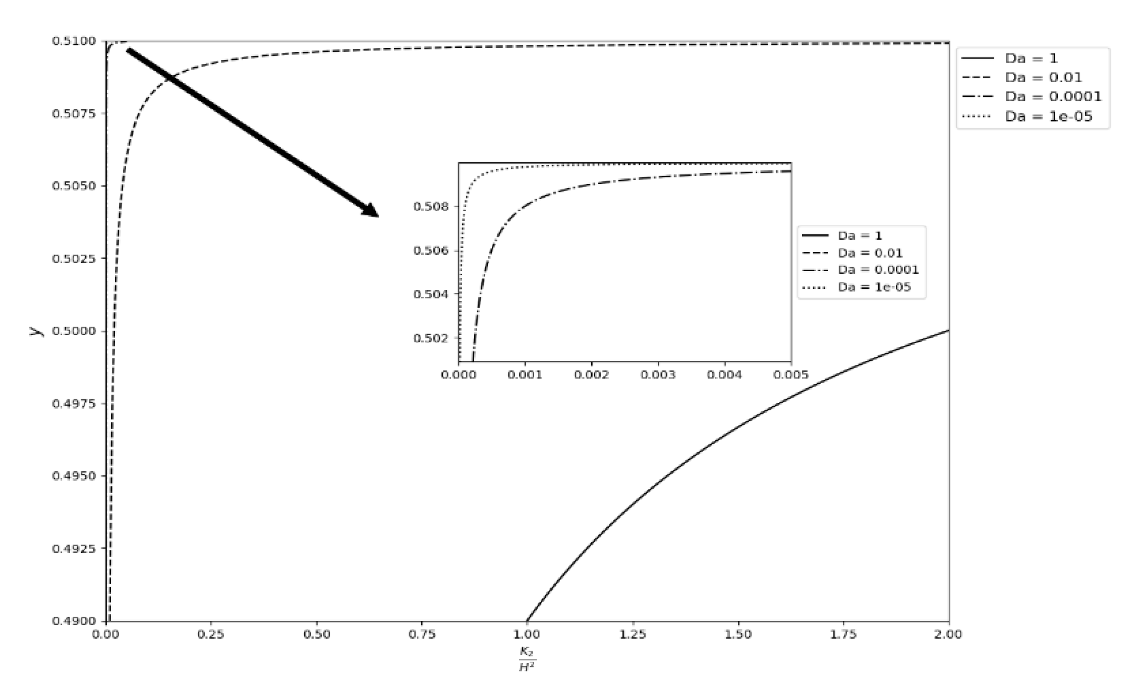
Figure 5.
Velocity Profiles in the Thin Layer. n=1 and Low Values of Da.
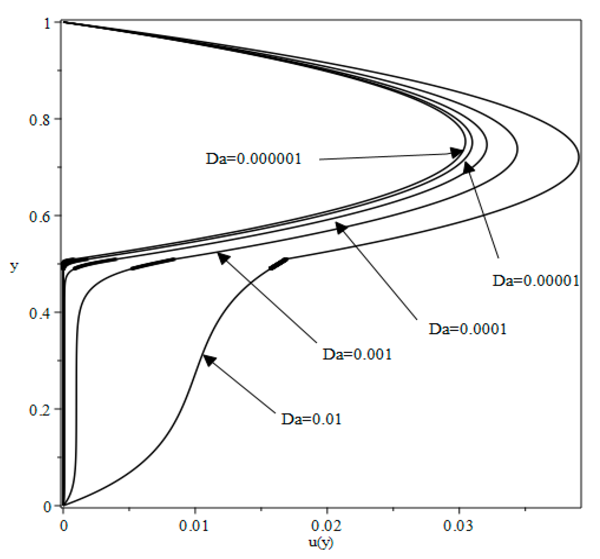
Figure 6.
Velocity Profiles in the Thin Layer. n=2 and Low Values of Da.
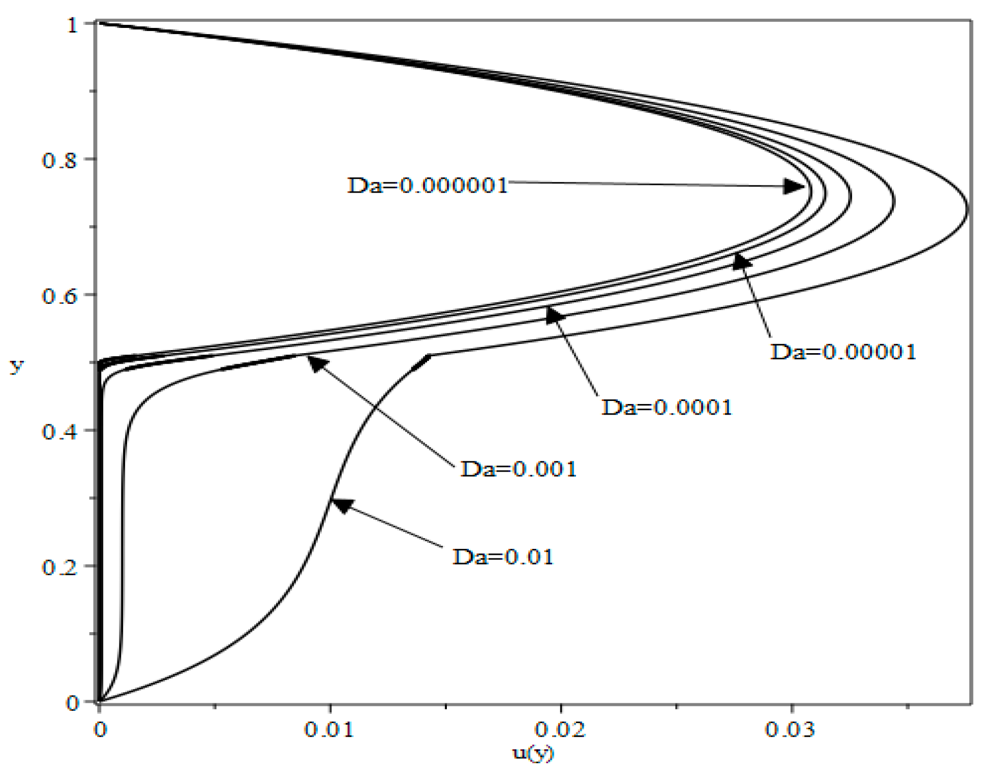
Figure 7.
Velocity Profiles in the Thin Transition Layer. Da = 0.0001 and Various Values of n.
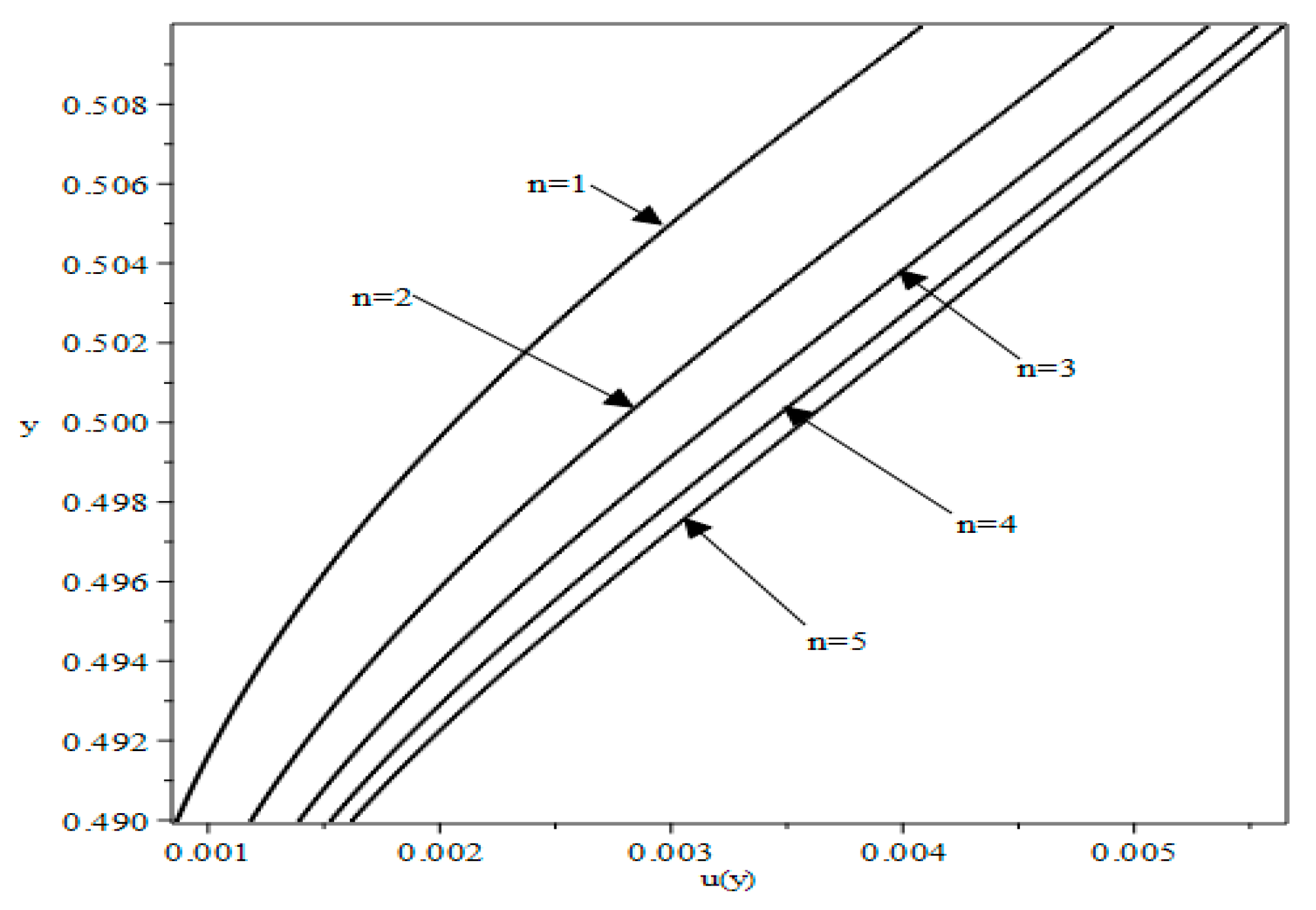

Table 1.
Flow equations for different parameters.
| Parameters | Flow Equation |
|---|---|
| Navier-Stokes equations | |
| Darcy’s equation | |
| Brinkman’s equation | |
| Forchheimer equation |
Table 2.
Velocity at the Upper Interface for Thick Layer.
| n | Da=0.01 | Da=0.001 | Da=0.0001 | Da=0.00001 | |
|---|---|---|---|---|---|
| 1 | 0.02114994 | 0.01233274 | 0.00649720 | 0.00321735 | |
| 2 | 0.02486639 | 0.01738999 | 0.01133148 | 0.00699674 | |
| 3 | 0.02673316 | 0.02050963 | 0.01498183 | 0.01049763 |
Table 3.
Velocity at the Lower Interface for Thin Layer.
| n | Da=0.01 | Da=0.001 | Da=0.0001 | Da=0.00001 | |
|---|---|---|---|---|---|
| 1 | 0.01570451 | 0.00521685 | 0.00086581 | 0.00002779 | |
| 2 | 0.01359440 | 0.005336297 | 0.0011867 | 0.00006497 | |
| 3 | 0.01217774 | 0.00526991 | 0.00139504 | 0.00011395 |
Table 4.
Shear Stress at upper and lower interfaces.
| Upper Interface |
Da=0.01 Thin Layer |
Da=0.01 Thick Layer |
|---|---|---|
| n=1 | 0.21053324 | 0.10321682 |
| n=2 | 0.21585593 | 0.09206747 |
| n=3 | 0.21940578 | 0.08646717 |
| Lower Interface |
||
| n=1 | 0.05854085 | 0.02721478 |
| n=2 | 0.03743739 | 0.04813607 |
| n=3 | 0.02326929 | 0.06526954 |
Table 5.
Mean velocity across the channel for n=1,2 and different Da.
| Thick Layer | Da=1 | Da=0.1 | Da=0.01 |
|---|---|---|---|
| n=1 | 0.07939500 0.0794* |
0.05692682 | 0.02071123 0.0207* |
| n=2 | 0.08744141 | 0.06403606 | 0.02670879 |
| Thin Layer | |||
| n=1 | 0.07940428 0.0794* |
0.05735128 | 0.02355505 0.0236* |
| n=2 | 0.07945951 | 0.05759342 | 0.0238459 |
*Nield and Kuznetsov [30] Results.
Disclaimer/Publisher’s Note: The statements, opinions and data contained in all publications are solely those of the individual author(s) and contributor(s) and not of MDPI and/or the editor(s). MDPI and/or the editor(s) disclaim responsibility for any injury to people or property resulting from any ideas, methods, instructions or products referred to in the content. |
© 2025 by the authors. Licensee MDPI, Basel, Switzerland. This article is an open access article distributed under the terms and conditions of the Creative Commons Attribution (CC BY) license (http://creativecommons.org/licenses/by/4.0/).
Copyright: This open access article is published under a Creative Commons CC BY 4.0 license, which permit the free download, distribution, and reuse, provided that the author and preprint are cited in any reuse.


