
Submitted:
14 April 2025
Posted:
15 April 2025
You are already at the latest version
Abstract
As global trade expands, container terminals face growing pressure to improve efficiency and capacity. During the process of loading and unloading containers, several inspections are performed with the urgent need to minimize delays. In this paper we explore corrosion, as it poses a persistent threat that compromises container durability and leads to costly repairs. Identifying this threat is no simple task, as it varies in form, progresses unpredictably, and is influenced by diverse environmental conditions and container types. In collaboration with the Port of Sines, Portugal, this work explores a potential solution for a real-time computer vision system, with the aim to improve container inspections using deep learning algorithms. We propose a system based on the semantic segmentation model, DeepLabv3+, for precise corrosion detection using images provided from the terminal. Given that the data was entirely raw and unprocessed, several techniques were applied for pre-processing, along with a review of various annotation tools. Once the data and annotations were prepared, we explored two approaches: leveraging a pre-trained model originally designed for bridge corrosion detection and fine-tuning a version specifically for cargo container assessment. Achieving performance results of 49% corrosion detection on the fine-tuned model, this work showcases the potential of deep learning in automating inspection processes and highlights the importance of generalization and training in real-world scenarios, exploring innovative solutions for smart gates and terminals.
Keywords:
smart ports
; corrosion detection
; computer vision
; deep learning
; semantic segmentation
; cargo containers
; data engineering
1. Introduction
Over the past decades, globalization has increased economic activity and international trade. As a result, the total volume of containers has grown at an average annual rate of 3.84%, leading to a substantial 56% increase in total volume from 2010 to 2022 [1].
Containers are standardized metal boxes, typically composed of Corten steel panels designed to protect cargo from harsh weather conditions and theft. Typically, they are designed in two main sizes: 20-feet-equivalent-unit (TEU) and 40-feet-equivalent-unit (FEU) with fixed width and length, and can have varying heights. This uniform structure makes them versatile for intermodal transport, allowing them to be properly loaded and stacked. They are typically composed with Corten steel surfaces and classified across several categories, such as general cargo, open-top, flat-rack, platform, refrigerated, and tank units. Each category is distinguished by unique attributes and structural designs that comply with the International Organization for Standardization (ISO) 1496 and 668 series, as well as related standards [2,3,4]. Containerization replaced traditional transportation methods, such as breaking bulk cargo, significantly reducing costs and loading times while maximizing cargo capacity. This transformation has enabled more cost-effective and efficient global trade connections [5].
Container terminals function as transfer stations for cargo flow and integrity control. Typically, terminals are composed of two external regions, the quayside where ships are loaded and unloaded, and the landside where containers are transferred to trucks and trains. Globalization and technological advancements have accelerated the growth of container terminals in seaports, requiring terminals to constantly adapt and look for innovative and efficient operational strategies. These solutions reduce transshipment times and costs, to maintain a smooth flow of logistic operations in ports. In response to this demand, the terminals continue to evolve to incorporate faster and more efficient technologies [2,3,4]. Smart gates contributed to the revolution of maritime ports in the way truck drivers process container pick-ups. Acting as integrated gate systems at entry and exit points, they optimize operations, procedures and security with the use of technologies such as sensors, cameras, optical character recognition (OCR) and artificial intelligence (AI) [6].
Inspection processes in container terminals and gates, such as code recognition, seal detection, and damage detection, are some of the operations prone to automatization. Containers are constantly exposed to harsh environmental conditions, heavy loads, and frequent handling, all of which contribute to wear and tear over time. Traditionally, inspections are based on a manual process with subjective judgment from trained professionals, making this conventional approach not only labor intensive and time-consuming, but also susceptible to human error and inconsistencies. Without regular and reliable monitoring, the chances that containers are exposed to damages increase, putting cargo integrity at risk. To minimize manual labor and increase efficiency, terminals are exploring Computer Vision (CV) solutions capable of performing autonomous inspections [7]. Computer vision technology allows devices to understand visual data as closely as possible to human perception. Through the use of imaging devices and algorithms, these systems can recognize patterns and anomalies within objects [8]. These algorithms require a large amount of prepared data to perform visual tasks. Based on the vast amount of data collected from port cameras in container terminals, with proper preparation, it is possible to perform automatic inspections using Deep Learning (DL) algorithms. Therefore, this technology allows the system to detect anomalies in containers, improving not only logistic operations but also the accuracy and reliability of inspections. Although these combined methods provide solutions and could revolutionize the whole sector, the port industry still faces notable challenges in fully deploying these systems [7].
This paper is structured as follows. Section 2 describes the methodology, including the pre-processing steps for building a custom dataset, a review of segmentation models, and the selection of the model for training and testing, along with the strategies and experiments conducted. Section 3 describes the experiment results, highlighting the performance of the proposed approach on several configurations. Section 4 discusses the findings, limitations, and potential improvements. Finally, Section 5 concludes the study and outlines directions for future work.
1.1. Related Work
Detecting defects on containers is challenging due to the complexity of the task, despite these challenges, some attempts were tested in this area. Wang et al. [9] proposed a multi-type damage detection model for shipping containers based on transfer learning and MobileNetv2. This model was trained in a dataset with the following classes: damage, hole, bent, dent, rusty, surrounding (port environment), open (door not closed), collapse (container stacks), and norm (normal container). This research uses the WESPE (Weakly Supervised Photo Enhancer) algorithm to enhance images for the dataset while also structuring a relationship map between low- and high-quality images. MobileNetv2 and Inceptionv3 were used as pre-trained models, with the original weights preserved. This model integrates feature extraction, global average pooling techniques, dropout regularization to avoid overfitting, and ultimately a classification layer that returns the predicted output. Subsequent to initial training, both MobileNetv2 and Inceptionv3 were subjected to post-training refinements with fine-tuning to improve the accuracy of the model. To conclude, the author claimed that the models were more suitable for the actual container detection situation at the port. His work allows the use of mobile devices to collect images and transmit them to a central unit. After experimenting results, the MobileNetv2 model had overall better generalization performance compared to the Inceptionv3 model. From the results, it seems the model struggled to distinguish the surroundings of a normal container image; however, with respect to damage classification, the results seem promising. Although the author left room for improvement, it led to an interesting proposal with good performance, capable of acting on the shipping industry.
Bahrami et al. [10] focused on detecting corrosion on shipping containers with two different approaches. Firstly, the author developed an optimized deep learning architecture with anchor box that relies on predefined bounding boxes (anchor boxes) to detect objects at different scales and ratios, leading to the detection of corrosion. This process improves performance and generalization, combined with the following networks: Faster R-CNN (Region-Based CNN), SSD (Single Shot Detector) Mobilenet, and SSD Inceptionv2. These architectures demonstrate their suitability to address the challenging task of detecting corrosion defects. Two experiments were proposed with anchor boxes, first with fixed-size boxes and another with flexible size. While performing the experiments, the fixed-size anchor box model failed to detect all corrosion defects and did not provide high performance. For the experiment where the anchor box size was flexible, there was an improvement over 5%. The faster R-CNN network showed better results than the SSD models. Despite these improvements, the three models did not provide solid results (within 90%) in terms of performance, as the best model achieved an accuracy of 66%. However, these advances have provided the shipping industry with a base framework for corrosion detection.
Lastly, Bahrami et al. [11] implemented a later approach that aims to address the challenges of generalization, which most models suffer to some extent. The proposed framework consists of two main modules: High resolution and temporal context (HRTC) region-based CNN (R-CNN) applied for corrosion defect detection and CDC (Corrosion Defect Characterization) for corrosion defect inspection. Initially, the first part of the framework incorporates a backbone network coupled with a Region Proposal Network (RPN) to generate corrosion proposal regions. These are subsequently refined, in the second phase, through the use of Region of Interest (ROI) Align to sharpen instance-specific features for classification and mask generation purposes. RPN includes a Multi Depth (MD) - Multi Scale (MS) Image Pyramid Network (IPN) that operates at varying depths and resolutions, implementing multiple CNNs. This results in a feature map from the MD-MS IPN wide range of scales and hierarchical levels, further enhanced through the integration of a MS-Featured Pyramid Network (FPN). Furthermore, with the camera setup not capturing the whole container in a single frame, the authors proposed to store all the key features from the improved FPN box proposals in memory banks. Using an attention mechanism, as assistance, the model prioritized important contextual information and ignored irrelevant data, combined with a short-term memory bank to consider temporal context on neighboring frames and a long-term memory bank that stores features from a wider range of frames to consider context over time. For the second part of the framework, CDC calculates the percentage of corroded areas on the container, using an optical flow to measure the displacement of sequential images and avoid overlaps. After determining full dimensions, edge detection techniques are used to define the boundaries, obtain the area, and calculate the percentage of pixels in corrosion regions. The precision of CDC in detecting corrosion in various weather conditions was shown to be above 88%, with a mean error between 5% and 11%. In conclusion, the proposed framework was compared with conventional segmentation techniques and metallic defect detection techniques. HRTC R-CNN outperformed every algorithm comparatively. This model proved to be the leading work in this sector with incredible performance results. Although the work of Bahrami et al. [10,11] provides significant progress in the domain of corrosion defect detection, it does not fully address the issue of generalization to other forms of damage. However, it lays the foundation for the potential adaptation of this methodology to a wider range of damage types.
2. Materials and Methods
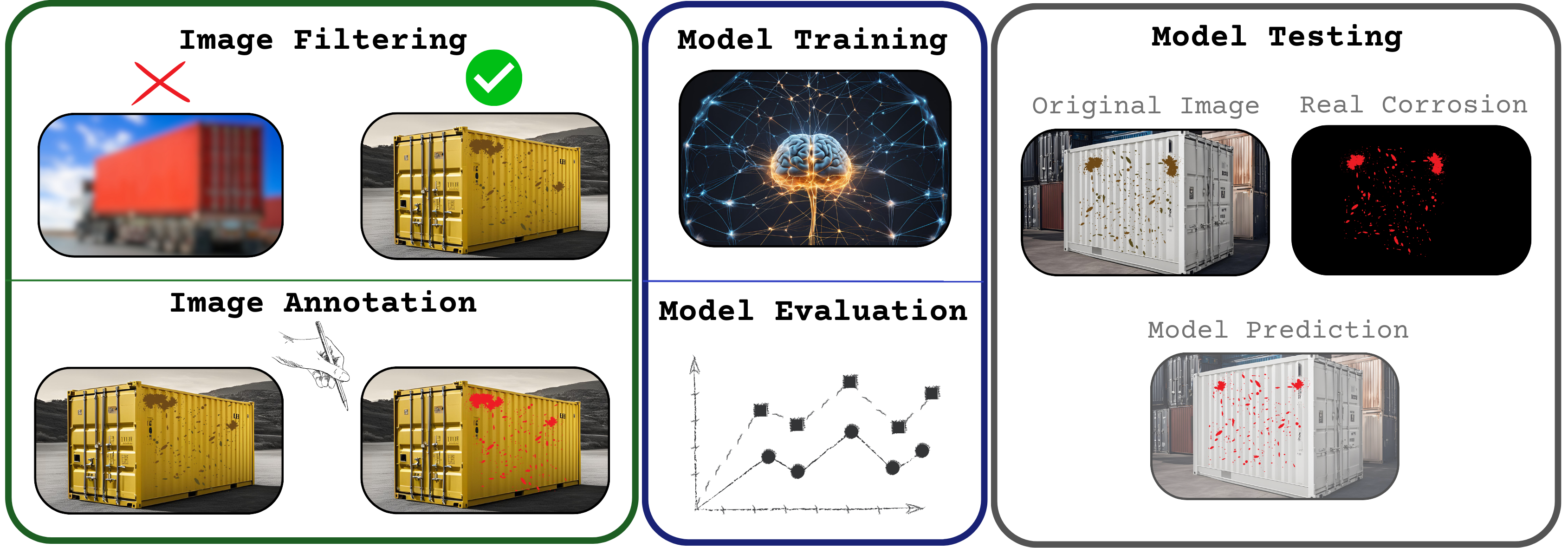
Deep learning (DL) tasks require annotated data to train and learn patterns. In semantic segmentation, the dataset must contain proper pixel-wise mask annotations. Preparing a suitable dataset is crucial for the success of the model; Without it, the model will not be able to learn patterns within the data and generalize to new samples. To build an algorithm capable of accessing real-time image input, the following steps were necessary to prepare the data:
- Pre-processing of raw data.
- Data annotation.
- Data splitting.
- Data rescaling.
After ensuring a proper balance of the data, several experiments were performed with the DeepLabv3+ model. In conclusion with an evaluation of the model performance in a new set of images, we analyze its ability to adapt to new scenes.
2.1. Data Preparation
In order to obtain a more generalized dataset with a wider variety of containers, an attempt to retrieve data from authors of similar research was made. However, the response was not positive, as the data was classified and could not be shared with the scientific community. Leading to the next step of searching for public datasets, where, the data found was not reliable, as it was composed of images from different natures with low quality, composed with water marks, proving to be unsuitable for DL models. Furthermore, the retrieved data from PSA Sines, had no treatment nor criteria, as it consisted of images from straddle carriers with low criteria for DL models. This showcased the need to filter and pre-process the provided data, mostly, blurry and noisy images.
2.1.1. Pre-Processing
Two image processing techniques were applied to detect blur and noise: Laplace operator and Canny Edge Detector [12,13]. The Laplacian operator is a second-order derivative operator that uses a similar concept to the Sobel operator. Unlike the Sobel operator, which detect edges by calculating an approximation of the intensity gradient at each pixel, the Laplacian operator calculates the rate of change of the gradient. Laplace operator is defined by the following Equation (1):
To explain further, the Sobel operator identifies pixels with large intensity changes while the Laplace operator detects edges by finding zero-crossings. This difference is illustrated in Figure 1.
Before applying the filter, the image was converted to grayscale and the Laplacian values were calculated for each image. An example of a good and rejected image with the filter applied can be seen in Figure 2.
Canny Edge Detection is a multi-stage algorithm that detects strong edges in images. Firstly, it calculates the intensity gradient of the image, similar to Sobel, as seen in Equation (2):
It then calculates the direction of the gradient with the following Equation (3):
Afterwards, it uses non-maximum suppression to remove non-significant pixels by comparing each pixel gradient with its neighbors in the gradient direction, keeping only the local maxima. This ensures sharp and thin edges after checking every pixel. Lastly, hysteresis thresholding is applied to compare the gradient values with the two thresholds: lower and upper. If the gradient value is above the upper threshold, it is considered a strong edge pixel. If it is below the lower threshold, it is considered a non-edge pixel. The values in between are considered weak edge pixels, that are kept only if they are connected to strong edge pixels, as seen in Figure 3, where edge B is discarded and edge C is valid.
Based on several tests performed with different image samples, the values for the thresholds were set to 50 and 150, with a ratio of 3:1 between them, and a kernel size of 3. An example of a good and a rejected image with the filter applied can be seen in Figure 4.
To conclude, based on the threshold defined from the two image processing techniques, the images that did not meet the criteria, were removed. Selecting a proper threshold value is an arduous task, as it either removes too many acceptable images or keeps too many rejected images. After several tests, since the amount of data provided was immense, the boundaries were defined with a broad margin, as represented in the following Equation (4):
All the data inside the defined threshold was rejected. These values were chosen based on the analysis of several light conditions and camera perspectives. An example of images used for training is represented in Figure 5, and rejected images in Figure 6.
Based on the previous examples, the following Table 1 represents the number of edge pixels and Laplacian values for the images shown in Figure 5 and Figure 6.
After completing the filtering process, the next step in preparing images for training the DL model involved annotations. Leading to a brief review of recent annotation tools. This evaluation led to the selection of the most practical tool for annotating corrosion masks.
2.1.2. Annotation
Crucially, this process is of extreme importance for the model, as it defines the ground truth of corrosion found in all the container data. These defined annotations are used to train the model to recognize the corrosion in the images. It can be done in different ways, such as bounding boxes or pixel-level labeling. In this work, it was used pixel-level labeling, since it is a segmentation task and it provides more detailed information. Annotation tools are very helpful on this process and they can be generic or specific for a particular task. To understand which tool is the most suitable, an analysis and testing of the available tools was performed. This analysis was based on self-testing, reviews, surveys and recommendations from the community [14,15,16], such as CVAT [17], LabelStudio [18], LabelBox [19], VIA [20] and LabelMe [21]. A comparison regarding generic features of these tools is presented in Table 2.
All of the tools analyzed are open-source, though some also offer premium versions with additional features. A key aspect considered during the analysis was the user-interface and its ease of navigation, which is important for time-limited projects. Another significant feature that was considered was the ability to handle large-scale datasets due to some tools struggling with handling large data. Lastly, and the most relevant feature considered, was the support of pixel-level labeling, given that it is the annotation type used in this work.
In terms of annotation tools for CV tasks, only the most relevant ones were considered for this project, such as brush tool, AI magic wand, intelligent scissor, bounding box, and points. Brush tool gives the user free control to draw the annotation mask, while the AI magic wand uses AI to predict the annotation mask. Intelligent scissor allows the user to add points around the object, and the tool will automatically detect the object. Bounding box is more related to object detection, the user has to draw a box around the object while, with points, the user marks points on the boundaries of the object. From the analysis results the following comparison, presented in Table 3.
Most of the recent tools available, are pretty similar in terms of features. In this work, CVAT was used, as of the most recent tools, it had the most user-friendly interface and all the features needed for this project. An example of a fully annotated container is shown in Figure 7.
In this manner, 500 images were annotated, where 250 of those had corrosion present and the other 250 did not. This way, the model can learn to differentiate good containers from the corroded ones, balancing the data.
2.1.3. Rescaling Data
Considering that the images provided had a resolution of 3840x2160 pixels, and most models take as input 512x512 or 1024x1024, the following technique was used to resize the images to a proper resolution before being analyzed by the model. Thus, the resizing was done using the PIL library, which provides a variety of resampling filters. These filters are used to determine how the pixels in the image are combined to create the new image. Given that the quality of the images is relevant to the task, based on the following Table 4, which shows the quality of the downscaling and upscaling of the images, the LANCZOS filter was chosen for the resizing process.
2.1.4. Data Splitting
Upon completing the annotation process, the data was divided and balanced equally in terms of corroded and non-corroded images for the train, validation and test set, where 80% was used for training, 10% for validation and 10% for testing. Regarding the criteria for corrosion annotation in the images, it was mainly based on the presence of rust, subjectivity of the annotator with guidance from collaborators. For a more precise annotation, a professional in the field of corrosion should be consulted to provide guidance on the annotation process. These annotations were then used to train the model.
2.2. Corrosion Segmentation
Based on the review and comparison performed of the semantic segmentation models, the DeepLab model demonstrated remarkable performance outperforming previous state-of-the-art models, as illustrated in Table 5.
2.2.1. DeepLabv3+ Architecture
DeepLab is a series of models that have been developed by the Google Research team, essentially formed by a Deep Neural Network (DNN), trained for image classification, and transformed into a Fully Convolutional Network (FCN). This is achieved by changing the fully connected layers into convolutional layers and increasing the feature resolution to the original input size with atrous convolution layers. DeepLabv3+ [25] introduced a decoder module to the Atrous Spatial Pyramid Pooling (ASPP) of the DeepLabv3 model, which was responsible for recovering spatial information lost during the encoding process. The extracted encoder feature resolution was freely controlled by atrous convolution, allowing the model to trade off precision and runtime. This structure is illustrated in Figure 8.
Based on these improvements, an illustration of the decoder effect compared to the previous bilinear upsampling method, used in the DeepLabv3 version, is shown in Figure 9.
In Figure 9, it can be seen that the decoder module is able to recover the spatial information lost during the encoding process, providing a more accurate segmentation result. DeepLabv3+ model has several parameters that can be adjusted to improve the model performance in training. The main parameters tested were model backbone networks, output speed, epochs, batch size, and learning rate. It is also important to mention that the model already incorporates data augmentation using random scales, crops, and horizontal flips, improving model generalization to unknown environments. To evaluate the model performance and compare the predicted mask with the real mask, the Intersection over Union (IoU) metric was used. This metric quantifies the intersection of two masks by calculating the ratio of the overlap area to the union area, as represented in Figure 10. A higher IoU value indicates closer agreement between the predicted and real masks, reflecting improved model accuracy.
2.2.2. Background Extraction
To achieve background subtraction, a simple transformer architecture with a memory encoder called Segment Anything model (SAM) [26] was used. This model aims to segment any object in an image, regardless of its size, shape, or appearance. It supports segmentation through prompts, which are simple instructions passed to the mask decoder that is capable of outputting segmentation masks in real-time.
Initially, the images were processed with the automatic mask generator. SAM returns all the masks in binary format, where the object is represented by white pixels and the background by black pixels, and creates a file with several parameters, mainly, the area of the mask, the stability score and the bounding box. To find the container in the image, the mask with the largest area was considered. Resulting in a new image where only the container is visible. Regarding the background, two options were tested, black, which is the default color, and white, which is obtained by inverting the binary mask. The initial results of the pre-processing steps are shown in Figure 11.
This method proved unreliable, since it was observed that in some cases the model would segment the outside area which was higher than the container area and fail to extract the background.
2.2.3. Points as Prompt
In order to solve the aforementioned issue, instead of the automatic mask generator, two points were used, as a prompt, to guide the model in segmenting the container. In the following figures, the points used as prompt and the results of the model prediction are shown. This method was successful in isolating the container from the background, as shown in Figure 12.
Although the model was able to segment the container from the background, it was observed that the model struggled to segment the borders of the container correctly. To avoid misjudging the container with the annotations, an erosion operation and a dilation operation were applied to the mask.
Both of these operations were performed with the OpenCV library, using a 5x5 kernel. This kernel for the erosion operation only considers the pixel as 1 if all the pixels under the kernel are 1. For the dilation operation, it only considers the pixel as 1 if at least one pixel under the kernel is 1. This results in a mask that ensures that all borders are correctly segmented, as shown in Figure 13.
Both black and white backgrounds were tested against the normal background in the pre-trained and trained model, as will be discussed in the experimental section.
2.3. Pre-Trained Model Experiments
Before training the model on the prepared dataset, an attempt was made to explore alternative methods that would not require extensive time in the annotations. In this context, pre-trained models were a possible solution, since corrosion is similar in nature to other segmentation tasks, like metallic surfaces or bridges, despite not being trained on the dataset prepared.
Four variations of a DeepLabv3+ pre-trained model were available, each trained in 440 images for bridge inspections, with different loss functions [27]. These four models were trained for 40 epochs with image sizes of 512x512, a batch size of two, horizontal flip augmentations, a ResNet50 backbone, and different loss functions. To distinguish between the models, they were denoted as w18, w27, w35 and w40, respectively. The different loss functions used were the following:
- w18: Cross entropy loss.
- w27: L1 loss.
- w35: L2 loss.
- w40: Cross entropy loss with weighted classes.
Before obtaining the results, some experiments were performed to understand how well the DeepLabv3+ model would behave in different scenarios. Since the model was trained with input images of 512x512 pixels, the first step was to resize the images to this size using the method in Section 2.1.3. Afterward, to understand the model performance, three experiments with images from the provided data were conducted as follows:
- Experiment 1: 20 random images.
- Experiment 2: 40 images without red cargo containers.
- Experiment 3: 20 images with only red cargo containers.
All of these experiments were tested in different settings, as described in Section 2.2.2, to see if the model could generalize better. However, firstly, it was necessary to prepare the ground truth masks in order to evaluate the pre-trained model performance. All the experiments mentioned above were annotated with CVAT to obtain the ground truth masks and then evaluate the model prediction compared to the ground truth using the IoU metric.
According to initial experiments, the model fails to identify corrosion in red cargo containers. Since this process of degradation typically appears in nature as a brown or orange color, closely similar to the color of red cargo containers, the model struggles to differentiate between the two.
2.4. Pre-Trained Results
As mentioned previously, to measure the precision of the pixels, IoU is the best metric to classify the performance of the model. This was calculated using the Torchmetrics library [28], which provides a simple way to calculate the metrics with built-in functions. Based on observations from early experiments, it was noted that the model had difficulty identifying corrosion in red cargo containers. This proved to be a limitation of the model, as it was trained on a different dataset. Taking into account the experiments performed on the 3 data samples, the results can be seen in Table 6. The model performed better in the first two experiments, where images were randomly selected, compared to the third experiment, where only red cargo containers were selected. This is because the model cannot distinguish between red cargo containers and corrosion. It is also noticeable that the model performed better with a white or black background instead of the default. Considering the fact that the images used in the experiments also include corrosion in other elements and it was only annotated the presence of corrosion in the main container, replacing the background with a white or black color improved the model performance.
In addition, the model performed better with cross-entropy-weighted classes, as seen in the w40 percentage results. Performing around 20% IoU in the first two experiments, while in the third experiment, all variations performed poorly, achieving less than 3% IoU. Despite this and considering that it is a model trained for a different task, the results were better than expected for the first two experiments. From the results, we can compare the predictions against the ground truth masks, when the background is similar to the color of corrosion and when it is distinct, as seen in Figure 14.
Despite achieving low IoU values, it was expected, since semantic segmentation is a complex task due to pixel-by-pixel comparison. Considering all this, the pre-trained models were not used for the corrosion segmentation task, as the models were unprepared for the dataset used and were unable to distinguish containers from corrosion when the color is identical. Therefore, the next step was to train the model on the dataset prepared.
2.5. Fine-Tuned Model Experiments
To train the DeepLabV3+ model in the data set, previously described in Section 2.2.1, a Pytorch implementation of the model was used with transfer learning on the backbone networks, available in a GitHub repository [29]. Before starting the training process, the dataset was transformed to fit the shape and size of the input of the model.
2.5.1. Data Transformation
Firstly, since the model was pre-trained on PASCAL VOC and Cityscapes datasets, it was required to create a custom dataset class to load the images and masks. This class was created based on the Pytorch Dataset class, which requires the implementation of two functions: __len__ which returns the size of the dataset and __getitem__ that returns the image and mask of a specific index. For the __len__ function, the size of the dataset was returned by reading the number of images in the respective text file (Train/Val/Test). While for the __getitem__ function, both images and masks were read from the respective folders, using the PIL library. After that, the mask was converted to a binary mask, where all non-zero pixels were converted to 1, resulting in an input shape of [batch size, channels, height, width] and a mask shape of [batch size, height, width], with the following values for the data input: [12, 3, 1024, 1024] and mask: [12, 1024, 1024]. These input shapes were also transformed by the data augmentation applied to the data, which were:
- Random Resize: resize the image with a random scale;
- Random Crop: crop the image to the model input size;
- Random Horizontal Flip: flip the image horizontally;
- ToTensor: convert image and mask to a Pytorch tensor;
- Normalize: normalize the image tensor with the mean and standard deviation of the ImageNet dataset.
After these conversions, the shape and size of the data were checked to ensure that the model could receive the data correctly, resulting in the following values for the input of the data: [12, 3, 512, 512] and mask: [12, 512, 512].
2.6. Training Experiments
To further evaluate the performance of the models, a few experiments were conducted on the training set, which consisted of 400 images with 200 corroded images and 200 non-corroded images. These experiments were trained and evaluated with the respective partitioning of the data set, and the training plots were created using the Visdom library [30].
Firstly, the model was trained with the default configuration, without any adjustments, to check the performance of the model on the dataset. However, due to the limited memory of the Graphics Processing Unit (GPU), it was necessary to make a slight adjustment to the batch size, reducing it to 12, and adjusting the number of epochs to 300. Regarding the rest of the parameters, they were kept as default, with the following values:
- Network model: MobileNetV2.
- Output Stride: 16.
- Learning rate: 0.01.
- Loss Function: Focal Loss.
- Learning Rate Policy: Poly.
- Optimizer: Stochastic Gradient Descent (SGD).
Afterwards, based on a few parameters and techniques used in pretests, like various learning rates, batch sizes, loss functions, and output strides, a standard based model was used in the following experiments with the following configurations:
- Background: Normal, white background and black background.
- Data augmentation: With and without data augmentation.
- Network comparison: MobileNetV2, ResNet50 and ResNet101.
- Optimizer comparison: SGD, Adam and AdamW.
2.6.1. Default Configuration
Initially, since this implementation had MobileNetV2 as the default backbone, it was decided to train the model with this configuration, because it is a lightweight model that can be trained faster than the other backbones. Based on DeepLabv2 and DeepLabv3 experiments [31,32], the learning rate policy was set to Poly and the output stride was set to 16, respectively. The poly policy is defined in Equation (5) where the policy gradually decreases the learning rate over time using a polynomial function.
For the step policy, the learning rate is decreased by a constant factor at fixed intervals, as shown in Equation (6):
2.6.2. Background
From the experiments made in the pre-trained models, it was observed that changing the background had a significant impact on the model performance. Therefore, it was decided to test the model with three different backgrounds: normal, white and black. This pre-process step was previously described in Section 2.2.2.
2.6.3. Data Augmentation
Corrosion has a wide variety of sizes and shapes, therefore, it was decided to test the model with and without data augmentation to see if the model could generalize better with the transformed data. Since the transformations, already described in Section 2.5.1, had rescale and random crop, those same transformations could negatively impact the model performance, as it could remove important spatial information from the images.
2.6.4. Network Backbone Models
Unfortunately, the Pytorch implementation of the model only had the MobileNetV2 and ResNet50 and ResNet101 backbone available, so it was not possible to test the latest addition of the Xception. Despite this, ResNet50 and ResNet101 were tested to check if they could improve the performance of the model, as described in the DeepLabv3 article [32].
2.6.5. Optimizers
3. Results
These experiments were performed with different configurations to evaluate the behavior of the model, as described in Section 2.6. Based on these, the model performance was evaluated using the best weights from the validation and compared against the results of the test set. Lastly, of all experiments, the best model configuration was identified for the corrosion segmentation task.
3.1. Default Configuration
Firstly, the model was trained using the default parameters with small adjustments (batch size of 12 and 300 epochs). Analyzing the loss of the training set, the model was able to quickly learn the patterns in the training data, as shown in Figure 15. When comparing the training and validation loss in Figure 16, the model does not overfit, as the validation loss follows a pattern similar to the training loss. Around 100 epochs, the two losses stabilize and remain relatively low and stable, indicating that the model has converged.
Regarding the performance (IoU) of the model, the results are shown in Figure 17, showing a rapid increase in the initial epochs, indicating that the model was able to learn quickly. Around 100 epochs, the model begins to learn more slowly and begins to stabilize over 40% IoU. Following 250 epochs, the learning curve starts to fluctuate slightly, indicating that the model has reached its learning capacity with the current data and parameters.
3.2. Background
Initially, the background removal technique was considered due to the fact that in addition to the corrosion in the main container, there were other containers and other objects that could contain corrosion as well. This could potentially confuse the model and decrease its performance, since the annotations were made only on the main container. However, despite the improvements made in the pre-trained models, when the background was removed in the training experiments, the results were not as expected. The background removal technique did not improve the model performance, as shown in the smoothed graph represented in Figure 18.
Clearly, the white background had the worst convergence due to instability during the train, while the black background had a convergence similar to that of the normal background. Despite this, since there was no significant improvement in model performance, this technique was not used in the following experiments.
3.3. Data Augmentation
Sequentially, it was also tested whether the transformations predefined in the DeepLabv3+ model would actually affect or not the learning behavior of the model. This was because the transformations could remove important spatial information from the images, which could be crucial for the model to learn the patterns in the data. The results are shown in Figure 19.
Looking into the results, when applying transformations to the data, the model learns slower; however, it is able to generalize better and achieve slightly better performance. Without transformations, the model learned faster since the data patterns were simpler, but the learning curve stagnated relatively quickly, indicating that the model reached its learning capacity. Consequently, the transformations were kept in the following experiments, as it was observed that the model could generalize better with the transformed data.
3.4. Backbone Models
Subsequently, the model was tested with different backbone models, such as MobileNetv2, ResNet50, and ResNet101. Regarding the MobileNetv2 and ResNet50 models, the standard batch size of 12 and 300 epochs with a learning rate of 0.01 remained the same. However, for the ResNet101 model, the batch size was reduced to 4 due to increased memory usage, consequently adjusting the learning rate to 0.005, resulting in Figure 20.
Similarly to the article [32], ResNet101 proved to be superior to ResNet50. MobileNetv2, despite being the fastest model to train, was low in terms of performance compared to the ResNet101 model. With an increase of 5% in performance compared to the previous best model (default configuration), the ResNet101 model was able to achieve a better learning curve, despite being slower, increasing the performance to 46%. This led to the conclusion that the ResNet101 model was the most suitable for this training task and was used in the following experiments.
3.5. Optimizers
Lastly, the model was tested with different optimizers, SGD being the currently used one. An additional test was made with the Adaptive Moment Estimation (Adam) and Adam with decoupled weight decay (AdamW) optimizers to check if they could improve the model performance. However, since the two optimizers had a greater oscillation in the learning curve, the learning rate was reduced to 0.0002 for the Adam and AdamW optimizers. The results are shown in Figure 21.
Although the original article [25] does not include any other optimizer besides the SGD optimizer, Adam and AdamW improved the model performance quite significantly. Both optimizers were able to achieve a better learning curve compared to the SGD optimizer, with AdamW being less oscillatory compared to Adam. With an increase of almost 10% in performance compared to the previous best model (ResNet101 model), the AdamW optimizer was able to achieve 53% performance (IoU).
In conclusion of the training experiments, the best configuration of the model was the ResNet101 model with the AdamW optimizer, achieving a precision of 53% IoU. Resulting in the best model configuration for the corrosion segmentation task. This model includes the following parameters:
- Network model: ResNet101.
- Output Stride: 16.
- Learning rate: 0.0002.
- Learning Rate Policy: Poly.
- Optimizer: AdamW.
3.6. Model Evaluation
With the conclusion of the training, a comparison was made between the validation and the performance of the test set. The best weights of the validation process were used to evaluate the model in the test set, noting that the model was trained on the training set and validated on the validation set to find the best weights. Subsequently, for each new experiment, the best performing model from the previous experiment was selected, as seen in Table 7.
Although in early experiments comparing the validation and test set, the model struggled to generalize, with a drop of 10% in the performance, ResNet101 was able to generalize slightly better, with a drop of only 6% in the performance. Further improvements were made with the AdamW optimizer, with a drop of only 3% in the performance when testing the model.
4. Discussion
Semantic segmentation is a challenging task and model performance can be influenced by several factors. In this section, the impact of the different configurations and hyperparameters used to train the model will be discussed. Despite the promising results obtained, it is also important to highlight that the model performance can be influenced by the quality of the dataset, since the annotations were made manually and can contain errors. Additionally, with only 500 images, the model may not have enough data to learn the patterns in the images, which can also influence the model performance. Furthermore, the quality of the images can also impact the model performance, since the images were taken in different lighting conditions, with different cameras, and with low resolution.
Based on the previous challenges, it is important to understand that achieving a high performance in detecting corrosion is not trivial, as the task is complex due to the variety of shapes and colors and the model needs to learn pixel by pixel the patterns in the images. Adding this to the low quality of the dataset, the task becomes even more challenging. However, the results were promising, especially since this is a new technology for this specific task. This result is significant considering the constraints and challenges faced during the development of the model. Regardless of these, the model performance can be further improved by increasing the dataset size and improving the quality and variety of the images and annotations. Additionally, by using more advanced techniques that require more computational power, such as using more complex models, smaller output strides, and increased resolution input images, the model performance can also be increased.
Furthermore, several examples of predictions during the validation process can be observed in Figure 22.
Upon evaluating the finest model, several examples of predictions can also be visualized during the test process, as shown in Figure 23.
Overall, the model was able to achieve good results, which is apparent when comparing the ground truth and the predicted mask. Considering background class, the model was able to achieve a mean IoU (mIoU) of 76%, which is impressive considering the constraints related to the dataset size.
4.1. Background Class
Up until this point, only the corrosion class performance was considered for clarity sake. However, the background also plays a role in the performance evaluation, especially since the model also needs to distinguish this class. Therefore, it was decided to include the background class upon describing the results, in order to check the model performance in the whole image. The results can be seen in Figure 24.
As depicted in Figure 24, the model was able to achieve a mean IoU of 76%, which is a good result considering the complexity of the task.
4.2. Comparison with Pre-Trained DeepLabv3+
Concluding the analysis of the fine-tuned model, an additional comparison was made with the pre-trained DeepLabv3+ model. For the pre-trained model, the best overall configuration of the pre-trained experiments was used, as described in Section 2.4. This configuration was the pre-trained model with a white background using cross-entropy weighted classes.
Regarding the fine-tuned model, the best configuration from the fine-tuned experiments was used, as described in Section 3.6, with a ResNet101 backbone network using the AdamW optimizer with a learning rate of 0.002. As shown in Table 8, the fine-tuned model achieved an IoU of 49.4%, a significant improvement compared to the pre-trained model, which achieved an IoU of 4.0%.
Although the pre-trained model achieved low performance in detecting corrosion in cargo containers, it was expected since the model was trained on a different dataset, while the fine-tune model was trained in the proper dataset. This comparison highlights the importance of fine-tuning models on the specific dataset, as it can significantly improve the model performance.
5. Conclusions
This paper presents a comprehensive approach to address the challenges associated with the detection of corrosion in cargo containers using DL techniques. More specifically, detecting corrosion using semantic segmentation, as it can provide pixel-wise predictions, useful to detect the exact location of the damage. This work successfully achieved promising results despite facing notable challenges, such as dataset constraints, noisy data, and models generalization issues. A custom dataset was created from port terminal data, consisting of 500 annotated images (250 corroded and 250 non-corroded). Data were carefully processed and split for training, validation and testing. Annotation was performed using the CVAT tool, which was evaluated and selected for its efficiency and easy-to-use, accurate labeling. Primarily, two variants were tested, using the DeepLabv3+ architecture: one with pre-trained weights (from a bridge inspection dataset) and another trained and fine-tuned on the provided, filtered dataset. Although the pre-trained model demonstrated poor adaptability, achieving a modest performance of 22% in the first experiments and 4% in the custom dataset test set, the fine-tuned model trained on the custom dataset demonstrated a notable improvement, achieving 49% accuracy for the corrosion class and an overall accuracy of 76% when including the background class in the test set.
This result represents an important step towards automating corrosion detection in cargo containers, a task that traditionally relies on manual inspections, which are time-consuming, labor-intensive and prone to human error. Besides showcasing a possible pipeline to create a dataset with pre-processing steps and annotation tools, it also provides valuable insights into the challenges and opportunities of applying DL techniques to real-world problems in the logistics industry. Through systematic experiments, notable improvements were achieved and a performance baseline was established on which future studies could build on. Working with a small dataset and limited data diversity reflected the inherent challenges of working with real-world data. Particularly in container colors, lighting conditions and image resolutions had a clear impact on generalization. Although the fine-tuned model demonstrated promising results, more work is needed to improve performance to the levels required for real-world deployment. Despite these challenges, it provides a solid proof-of-concept and highlights clear solutions for future improvements. Importantly, the system demonstrates the potential to significantly reduce labor time, improve inspection reliability, and streamline logistics operations by automating a traditionally manual process.
5.1. Future Work
Several opportunities for future work have resulted from this work. Addressing these areas could improve model performance, generalization, and practical deployment. The following are potential directions for future research:
- Expand the dataset with more annotations: Increasing the number of annotated images, especially for corrosion and non-corrosion classes, could improve model robustness and performance. A wide variety of annotations would help the model learn new patterns and generalize better to unseen data.
- Improve data quality and diversity: As observed, certain container colors affected model performance due to data distribution discrepancies. Including a broader range of container colors, lighting conditions, and environmental settings could improve the accuracy and generalization of the model. Filtering out low-resolution images could also reduce noise and improve model performance.
- Experiment with alternative backbones: Testing alternative backbones, such as the Xception model, could reveal architecture-specific improvements. Xception is known for its efficiency in semantic segmentation tasks and may offer a better trade-off between performance and computational cost.
- Increase number of classes with other damage types: Although it was only addressed corrosion, extending the model to detect additional types of damage (dents or cracks) could increase its applicability in real-world scenarios. Training in multiple types of damage would provide a more comprehensive solution for cargo container inspections.
- Implement instance segmentation for multiple damage detection: Instance segmentation would allow the model to detect and label multiple occurrences of corrosion or other damage within a single image. This approach would provide more detailed information, especially in cases where it could be necessary to classify the severity of the damage.
- Develop a real-time damage detection system: Managing speed and efficiency is crucial for real-world applications. Integrating this system with a server-side application for reporting and archiving would facilitate a quick and effective damage assessment at port terminals.
In summary, this work addressed the challenge of creating a dataset from raw data and detecting corrosion in cargo containers using DL. Through the use of pre-processing techniques to build a dataset and training of a segmentation model, this work demonstrated the potential of DL techniques for damage detection. Although limitations remain, the results are promising given the complexity of the task and the constraints related to the size of the data set. By automating container inspections, this system has the potential to streamline workflows, reduce human error, and provide a quick assessment of container conditions. Ultimately, the benefits are for port terminal operations, logistics companies, and the shipping industry as a whole. Future research based on this work can focus on addressing the shortcomings highlighted, enhancing performance, and transitioning to real-time solutions that meet the demands of real-world applications.
Author Contributions
Conceptualization, D.O., D.C, A.J.R.N.; methodology, D.O, D.C.; software, D.O.; validation, D.O., D.C, A.J.R.N.; formal analysis, D.O., D.C, A.J.R.N.; investigation, D.O.; resources, A.J.R.N.; data curation, D.O.; writing—original draft preparation, D.O.; writing—review and editing, D.O., D.C, A.J.R.N.; visualization, D.O.; supervision, D.C, A.J.R.N.; project administration, A.J.R.N.; funding acquisition, A.J.R.N.. All authors have read and agreed to the published version of the manuscript.
Funding
This study was funded by the PRR—Recovery and Resilience Plan and by the NextGenerationEU funds at Universidade de Aveiro, through the scope of the Agenda for Business Innovation “NEXUS: Pacto de Inovação—Transição Verde e Digital para Transportes, Logística e Mobilidade” (Project no. 53 with the application C645112083-00000059). This work was also supported by the research unit IEETA (UIDB/00127/2020).
Data Availability Statement
The data presented in this study are available on request from the corresponding author. The data are not publicly available due to privacy issues.
Conflicts of Interest
The authors declare no conflicts of interest.
Abbreviations
The following abbreviations are used in this manuscript:
| Adam | Adaptive Moment Estimation |
| AdamW | Adam with decoupled weight decay |
| AI | Artificial Intelligence |
| ASPP | Atrous Spatial Pyramid Pooling |
| APS | Port of Sines Authority |
| CDC | Corrosion Defect Characterization |
| CNN | Convolutional Neural Network |
| CV | Computer Vision |
| DL | Deep Learning |
| DNN | Deep Neural Network |
| FCN | Fully Convolutional Network |
| FEU | Forty-feet-Equivalent-Unit |
| FPN | Feature Pyramid Networks |
| GPU | Graphics Processing Unit |
| HRNet | High-Resolution Network |
| HRTC | High-Resolution and Temporal Context |
| IoU | Intersection over Union |
| IPN | Image Pyramid Network |
| ISO | International Organization for Standardization |
| MD | Multi-Depth |
| mIoU | mean IoU |
| MS | Multi-Scale |
| OCR | Optical Character Recognition |
| R-CNN | Region Based CNN |
| RPN | Region Proposal Network |
| ROI | Region of Interest |
| SAM | Segment Anything model |
| SGD | Stochastic Gradient Descent |
| SSD | Single Shot Detector |
| TEU | Twenty-feet-Equivalent-Unit |
| WESPE | Weakly Supervised Photo Enhancer |
References
- United Nations Conference on Trade and Development (UNCTAD). Review of Maritime Transport 2024. United Nations publication (2024). Available online: https://unctadstat.unctad.org/datacentre/dataviewer/US.ContPortThroughput.
- Altunlu, O.; Elmas, G. Container Inspection and Repair Standards. Proceedings Book 2016, 404, İstanbul University. [Google Scholar]
- Carlo, H.J.; Vis, I.F.A.; Roodbergen, K.J. Transport operations in container terminals: Literature overview, trends, research directions and classification scheme. European Journal of Operational Research 2014, 236(1), 1–13. [Google Scholar] [CrossRef]
- Steenken, D.; Voß, S.; Stahlbock, R. Container terminal operation and operations research - a classification and literature review. OR Spectrum 2004, 26, 3–49. [Google Scholar] [CrossRef]
- Demil, B.; Lecocq, X. The Box: How the Shipping Container Made the World Smaller and the World Economy Bigger. M@n@gement 2006, 9(2), 73–79, Association Internationale de Management Stratégique. [Google Scholar] [CrossRef]
- Basulo-Ribeiro, J.; Pimentel, C.; Teixeira, L. Digital Transformation in Maritime Ports: Defining Smart Gates through Process Improvement in a Portuguese Container Terminal. Future Internet 2024, 16, 10. [Google Scholar] [CrossRef]
- Delgado, G.; Cortés, A.; Loyo, E. Pipeline for Visual Container Inspection Application using Deep Learning. International Joint Conference on Computational Intelligence 2022, 1, 404–411. [Google Scholar] [CrossRef]
- Orhei, C.; Mocofan, M.; Vert, S.; Vasiu, R. End-to-End Computer Vision Framework. 2020 14th International Symposium on Electronics and Telecommunications, ISETC 2020 - Conference Proceedings 2020. [Google Scholar] [CrossRef]
- Wang, Z.; Gao, J.; Zeng, Q.; Sun, Y. Multitype Damage Detection of Container Using CNN Based on Transfer Learning. Mathematical Problems in Engineering 2021. [Google Scholar] [CrossRef]
- Bahrami, Z.; Zhang, R.; Rayhana, R.; Wang, T.; Liu, Z. Optimized Deep Neural Network Architectures with Anchor Box Optimization for Shipping Container Corrosion Inspection. 2020 IEEE Symposium Series on Computational Intelligence, SSCI 2020 2020, 1328–1333. [Google Scholar] [CrossRef]
- Bahrami, Z.; Zhang, R.; Wang, T.; Liu, Z. An End-to-End Framework for Shipping Container Corrosion Defect Inspection. IEEE Transactions on Instrumentation and Measurement 2022, 71. [Google Scholar] [CrossRef]
- OpenCV. OpenCV-Python Tutorials. Available online: https://docs.opencv.org/4.x/d6/d00/tutorial_py_root.html (accessed on 16 February 2024).
- Bansal, R.; Raj, G.; Choudhury, T. Blur image detection using Laplacian operator and Open-CV. Proceedings of the 5th International Conference on System Modeling and Advancement in Research Trends, SMART 2016 2017, 63–67. [Google Scholar] [CrossRef]
- de Sousa Reis, P.M.L. Data Labeling Tools for Computer Vision: A Review. PQDT-Global 2021. [Google Scholar]
- Sager, C.; Janiesch, C.; Zschech, P. A survey of image labelling for computer vision applications. Journal of Business Analytics 2021, 4(2), 91–110. [Google Scholar] [CrossRef]
- Aljabri, M.; AlAmir, M.; AlGhamdi, M.; Abdel-Mottaleb, M.; Collado-Mesa, F. Towards a better understanding of annotation tools for medical imaging: a survey. Multimedia Tools and Applications 2022, 81(18), 25877–25911. [Google Scholar] [CrossRef]
- CVAT.ai Corporation. Computer Vision Annotation Tool (CVAT). Zenodo 2024. [Google Scholar] [CrossRef]
- Tkachenko, M.; Malyuk, M.; Holmanyuk, A.; Liubimov, N. Label Studio: Data labeling software. 2020-2024.
- Labelbox. The data factory for AI teams. Available online: https://labelbox.com/.
- Dutta, A.; Zisserman, A. The VIA Annotation Software for Images, Audio and Video. Proceedings of the 27th ACM International Conference on Multimedia (MM ’19) 2019. [Google Scholar] [CrossRef]
- Russell, B.C.; Torralba, A.; Murphy, K.P.; Freeman, W.T. LabelMe: A database and web-based tool for image annotation. International Journal of Computer Vision 2008, 77(1-3), 157–173. [Google Scholar] [CrossRef]
- Pillow Documentation. Pillow Handbook - Concepts. Available online: https://pillow.readthedocs.io/en/stable/handbook/concepts.html.
- Minaee, S.; Boykov, Y.; Porikli, F.; Plaza, A.; Kehtarnavaz, N.; Terzopoulos, D. Image Segmentation Using Deep Learning: A Survey. IEEE Transactions on Pattern Analysis and Machine Intelligence 2022, 44(7), 3523–3542. [Google Scholar] [CrossRef]
- Yu, H.; Yang, Z.; Tan, L.; Wang, Y.; Sun, W.; Sun, M.; Tang, Y. Methods and datasets on semantic segmentation: A review. Neurocomputing 2018, 304, 82–103. [Google Scholar] [CrossRef]
- Chen, L.-C.; Zhu, Y.; Papandreou, G.; Schroff, F.; Adam, H. Encoder-decoder with atrous separable convolution for semantic image segmentation. Lecture Notes in Computer Science (LNCS) 2018, 11211, 833–851. [Google Scholar] [CrossRef]
- Kirillov, A.; Mintun, E.; Ravi, N.; Mao, H.; Rolland, C.; Gustafson, L.; Xiao, T.; Whitehead, S.; Berg, A.C.; Lo, W.-Y.; et al. Segment Anything. arXiv 2023, arXiv:2304.02643. [Google Scholar] [CrossRef]
- Bianchi, E.; Hebdon, M. Development of Extendable Open-Source Structural Inspection Datasets. Journal of Computing in Civil Engineering 2022, 36(6), 04022039. [Google Scholar] [CrossRef]
- Detlefsen, N.S.; Borovec, J.; Schock, J.; Harsh, A.; Koker, T.; Di Liello, L.; Stancl, D.; Quan, C.; Grechkin, M.; Falcon, W. TorchMetrics - Measuring Reproducibility in PyTorch. Journal of Open Source Software 2022. February. [Google Scholar] [CrossRef]
- VainF. DeepLabV3Plus-PyTorch. 2022. Available online: https://github.com/VainF/DeepLabV3Plus-Pytorch.
- FOSSASIA. Visdom. Available online: https://github.com/fossasia/visdom.
- Chen, L.-C.; Papandreou, G.; Kokkinos, I.; Murphy, K.; Yuille, A.L. DeepLab: Semantic Image Segmentation with Deep Convolutional Nets, Atrous Convolution, and Fully Connected CRFs. IEEE Transactions on Pattern Analysis and Machine Intelligence 2018, 40(4), 834–848. [Google Scholar] [CrossRef]
- Chen, L.-C.; Papandreou, G.; Schroff, F.; Adam, H. Rethinking Atrous Convolution for Semantic Image Segmentation. arXiv preprint 2017. [Google Scholar] [CrossRef]
- Kingma, D.; Ba, J. Adam: A Method for Stochastic Optimization. International Conference on Learning Representations 2014. [Google Scholar]
- Loshchilov, I.; Hutter, F. Fixing Weight Decay Regularization in Adam. arXiv 2017. [Google Scholar] [CrossRef]
Figure 1.
Derivatives of the intensity of pixel edges [12].
Figure 1.
Derivatives of the intensity of pixel edges [12].
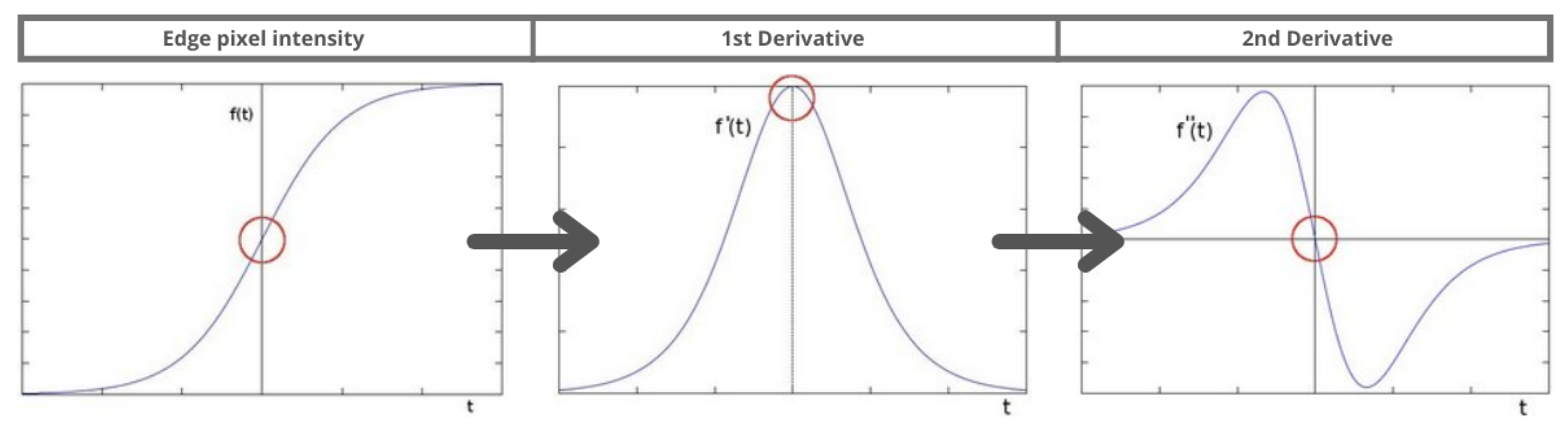
Figure 2.
Derivatives of the intensity of pixel edges [12].
Figure 2.
Derivatives of the intensity of pixel edges [12].

Figure 3.
Hysteresis thresholding. [12].
Figure 3.
Hysteresis thresholding. [12].
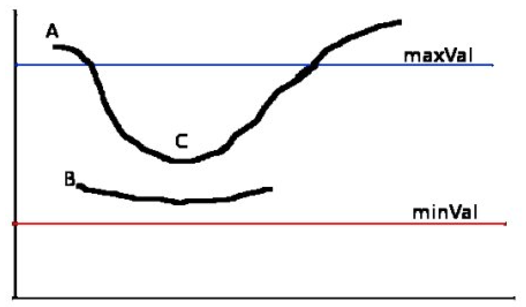
Figure 4.
Canny edge detection in selected and rejected examples.
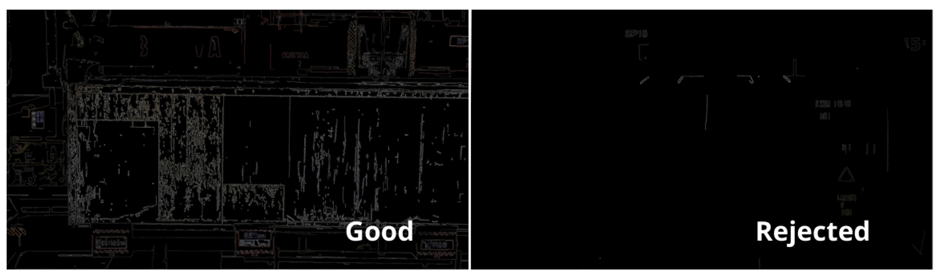
Figure 5.
Selected images for dataset.
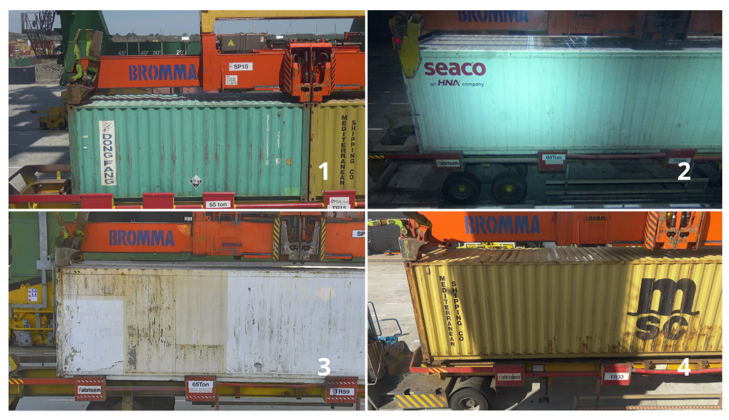
Figure 6.
Rejected images for dataset due to quality (1-2), blur (3) and brightness (4).
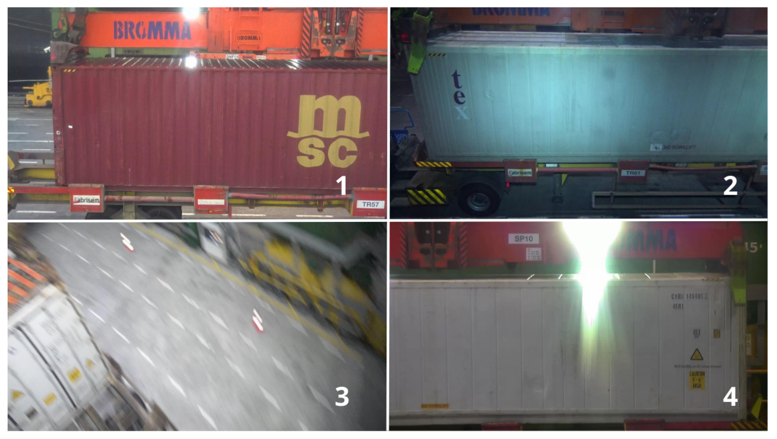
Figure 7.
Example of a fully annotated container.
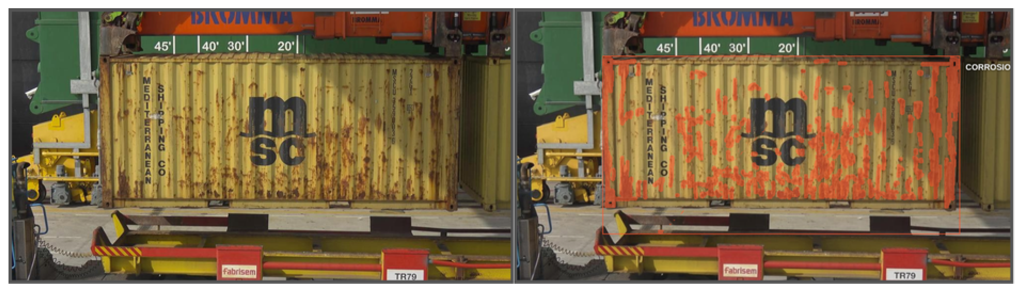
Figure 8.
DeepLabv3+ encoder-decoder architecture using ASPP for feature extraction and decoder for upsampling. Source from [25].
Figure 8.
DeepLabv3+ encoder-decoder architecture using ASPP for feature extraction and decoder for upsampling. Source from [25].
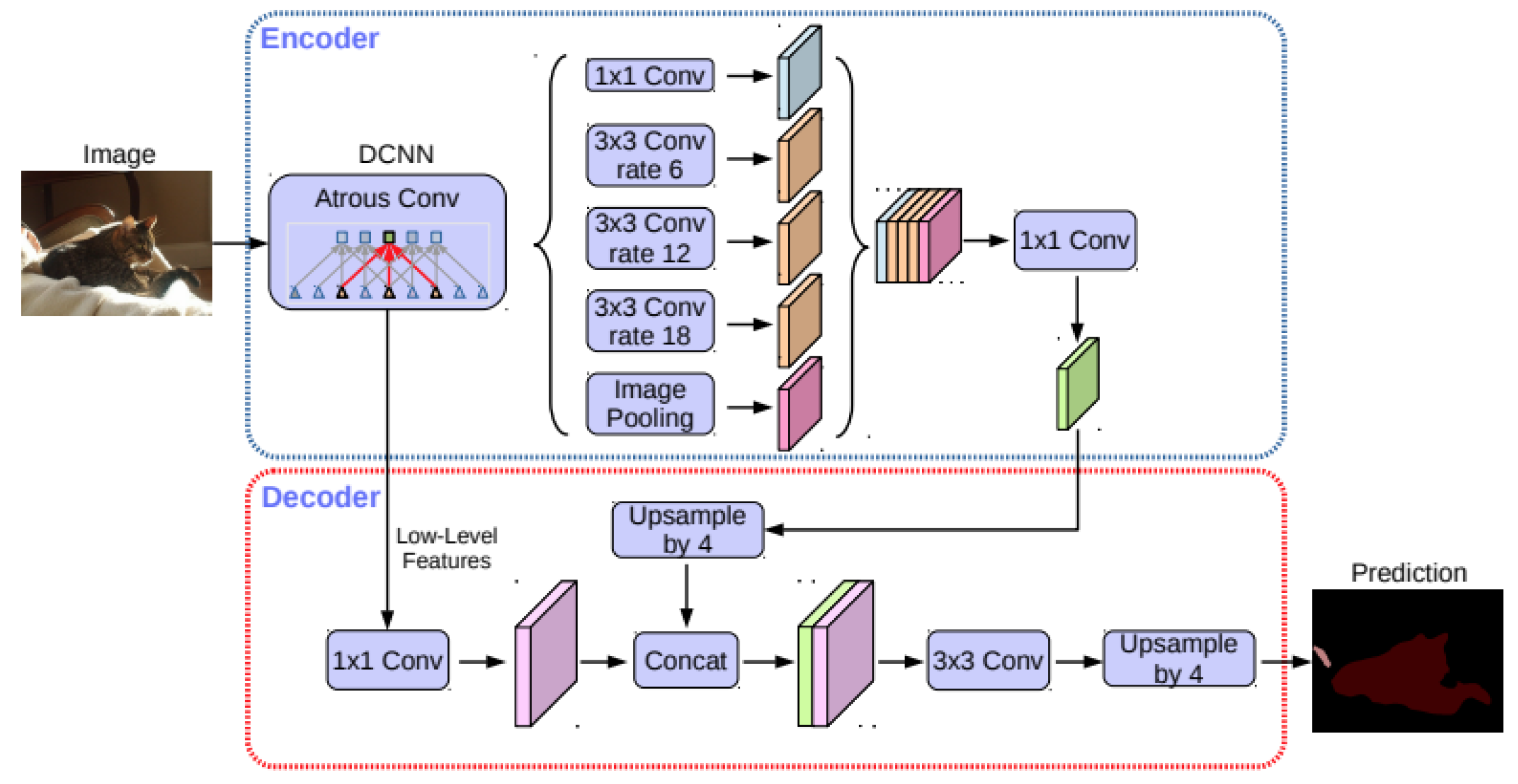
Figure 9.
Decoder effect compared with bilinear upsampling. Source from [25].
Figure 9.
Decoder effect compared with bilinear upsampling. Source from [25].
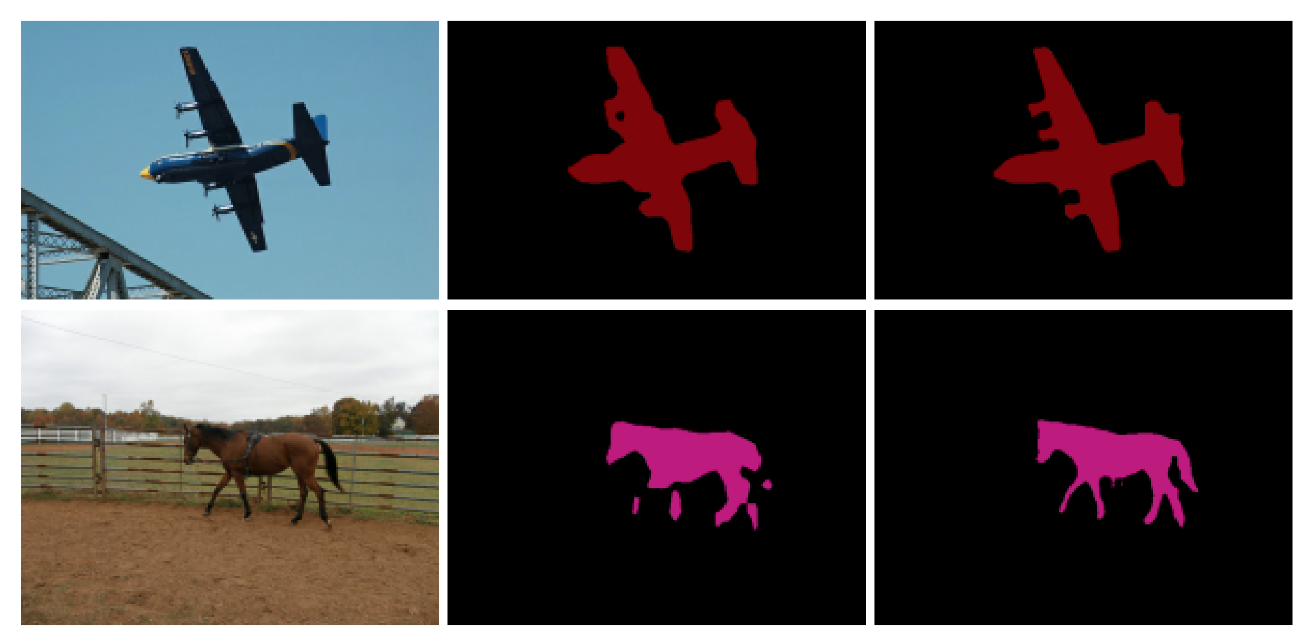
Figure 10.
Intersection Over Union metric.
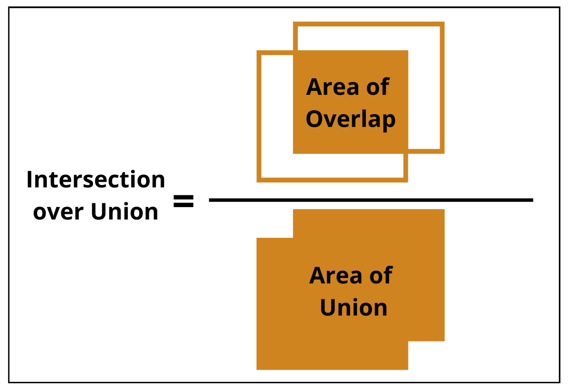
Figure 11.
Largest area segmented mask output from SAM.
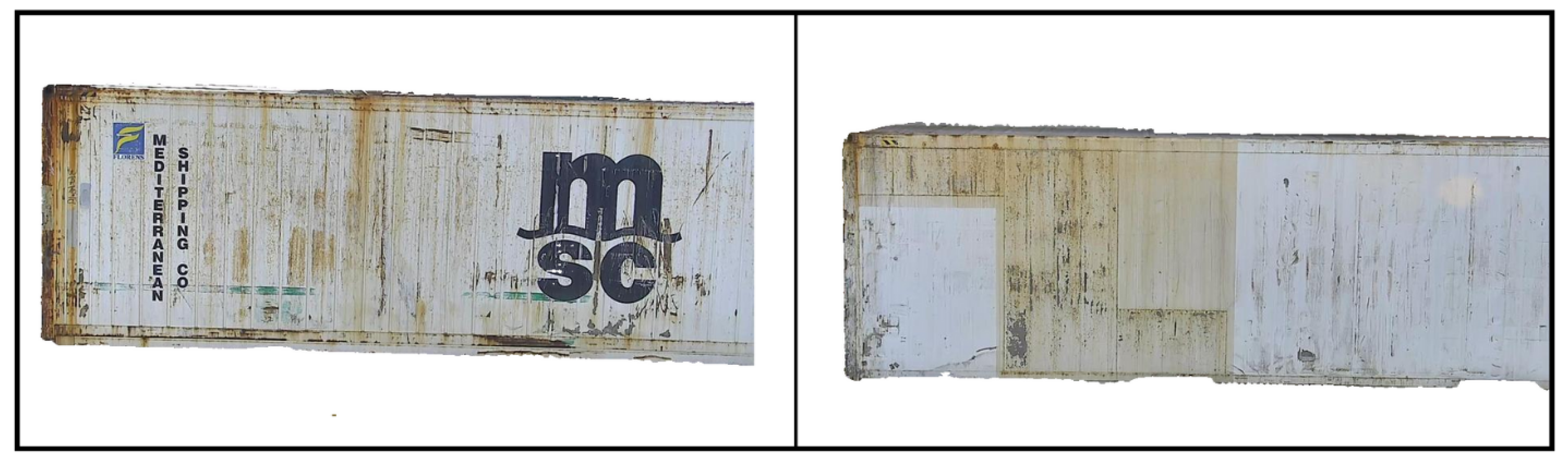
Figure 12.
Predictor output with 2 points (red star) as prompt. Best Mask Score: 0.975.
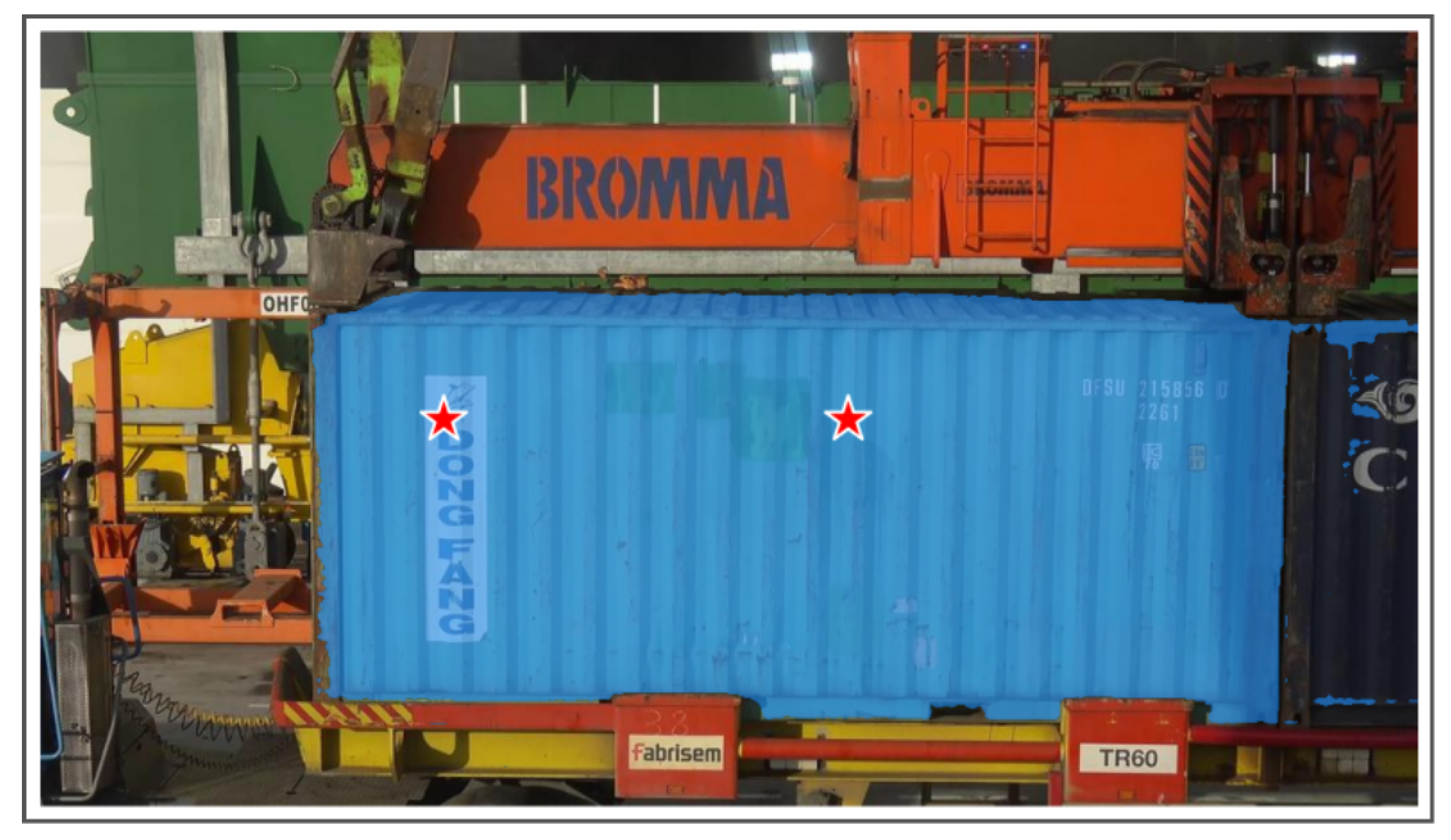
Figure 13.
Black and white background container masks.
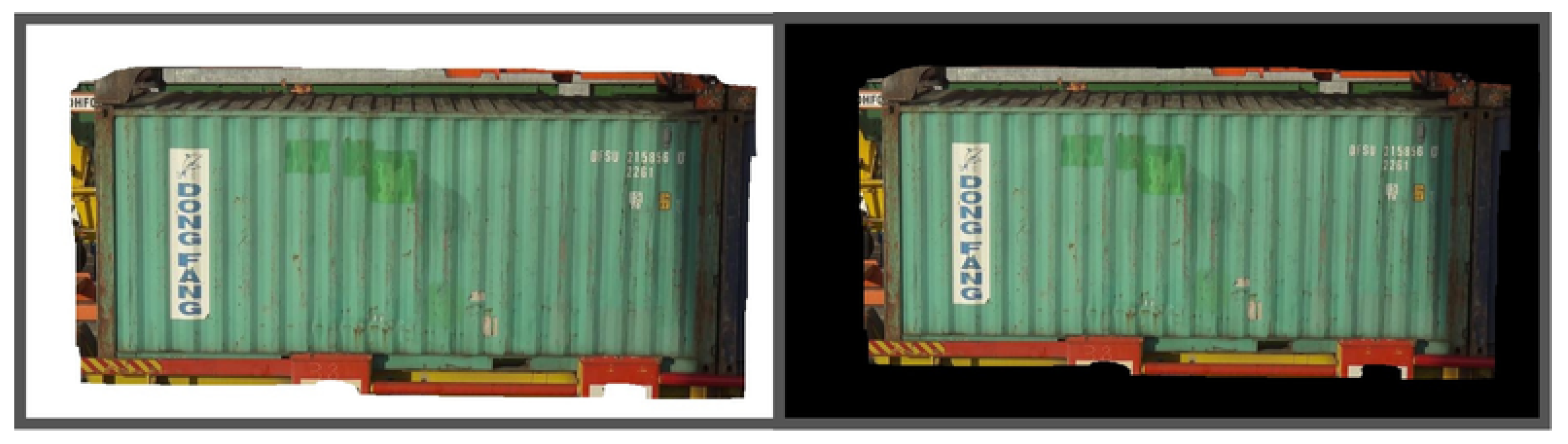
Figure 14.
Comparison of ground truth masks and model predictions for containers with distinct and similar corrosion colors.
Figure 14.
Comparison of ground truth masks and model predictions for containers with distinct and similar corrosion colors.
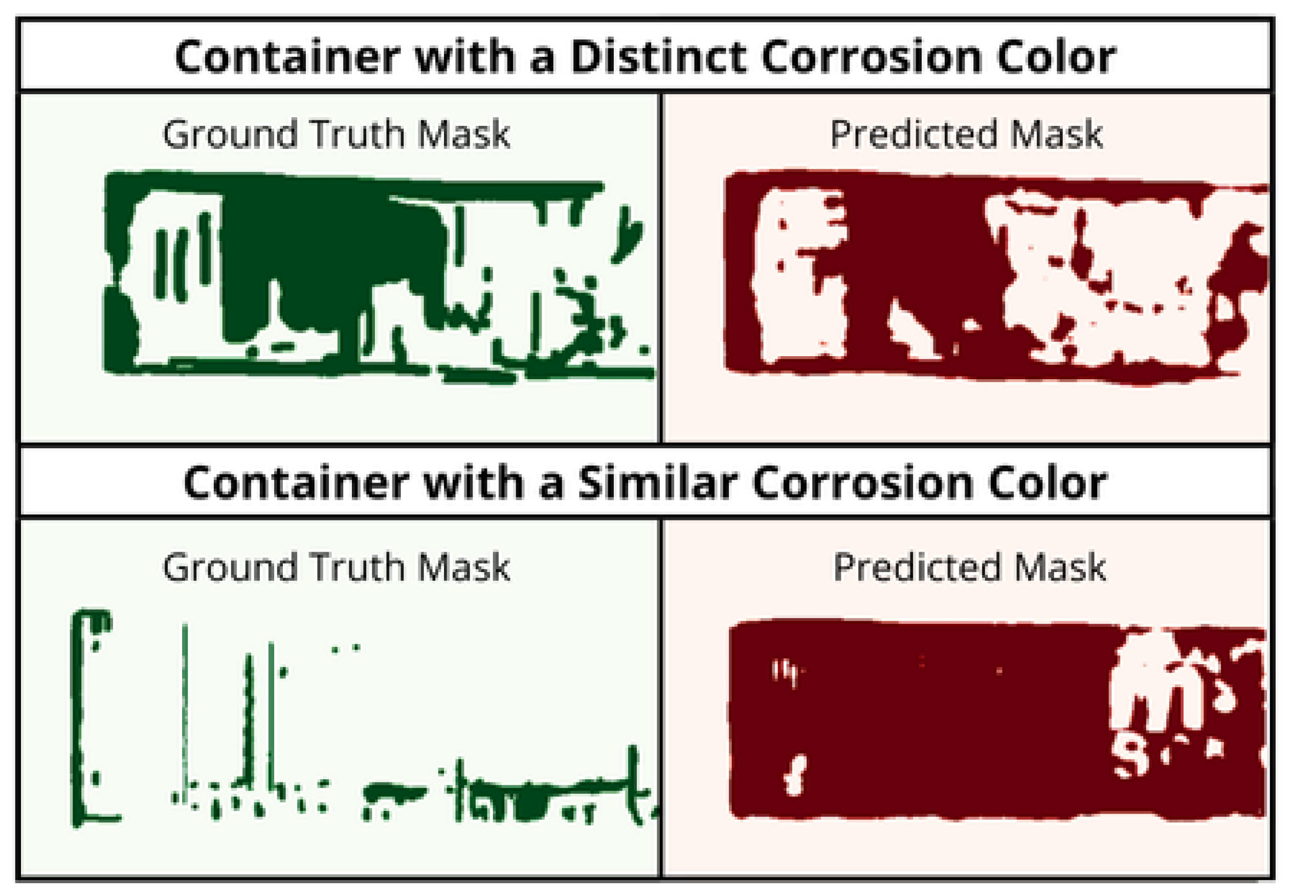
Figure 15.
DeepLabv3+: Training loss on 300 epochs using default parameters.
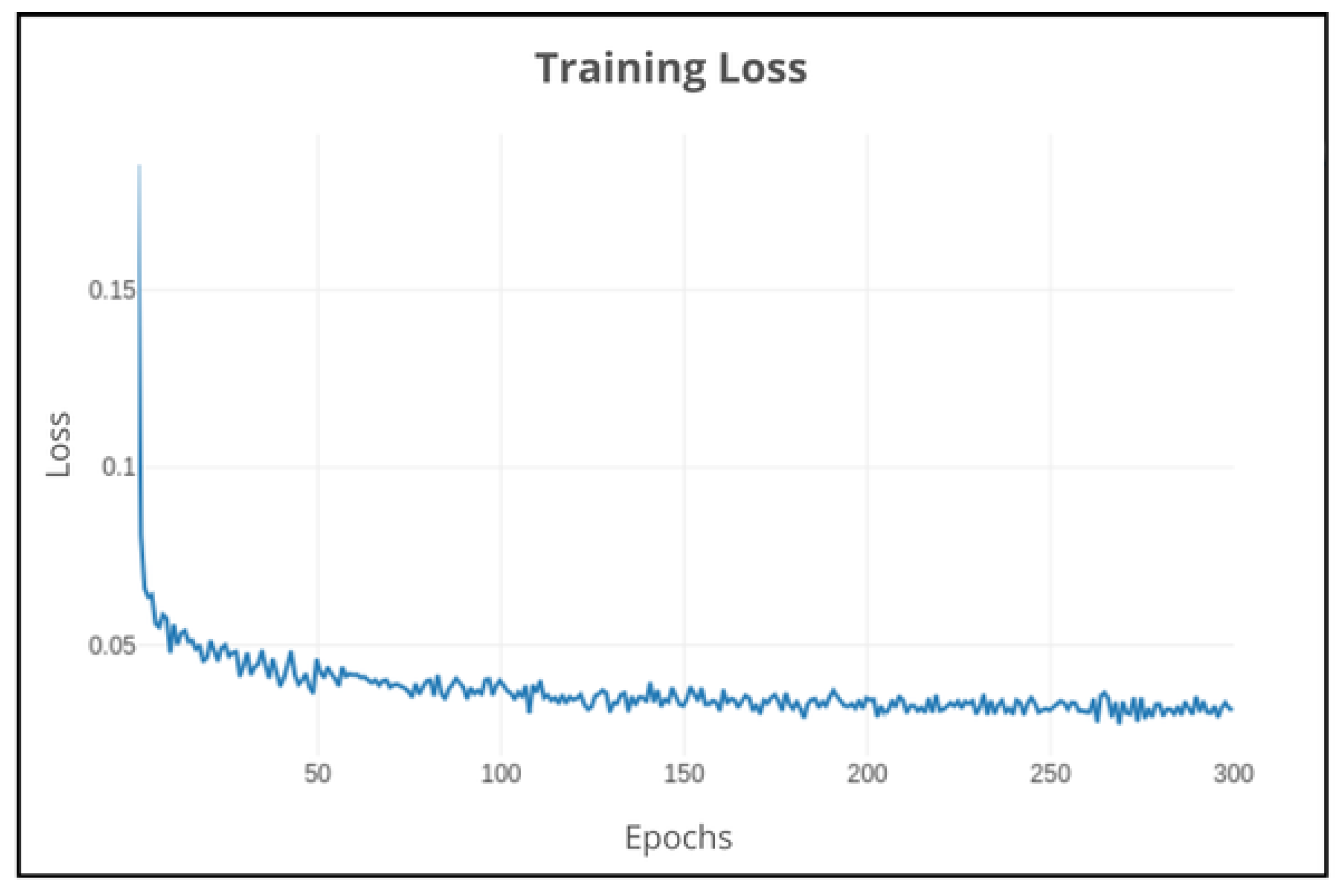
Figure 16.
DeepLabv3+: Validation loss on 300 epochs using default parameters.
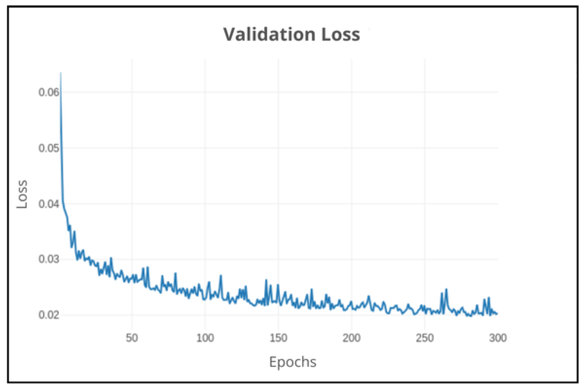
Figure 17.
DeepLabv3+: Validation performance of corrosion IoU on 300 epochs using default parameters.
Figure 17.
DeepLabv3+: Validation performance of corrosion IoU on 300 epochs using default parameters.
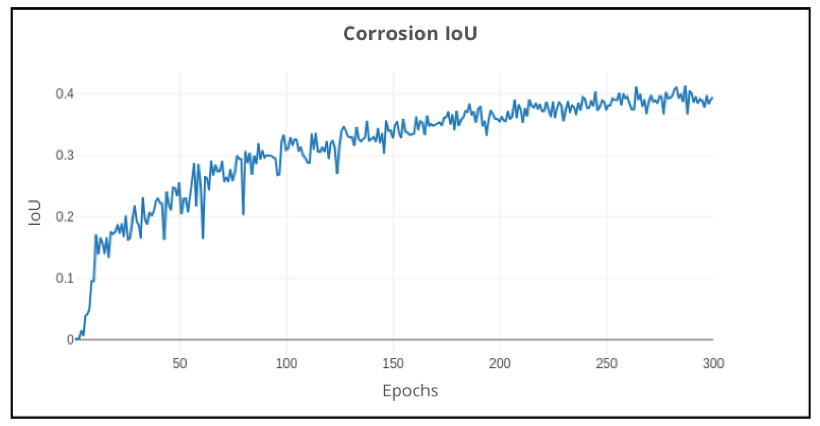
Figure 18.
DeepLabv3+ (smoothed lines): Impact on validation performance using different backgrounds (default, white and black) on 300 epochs.
Figure 18.
DeepLabv3+ (smoothed lines): Impact on validation performance using different backgrounds (default, white and black) on 300 epochs.
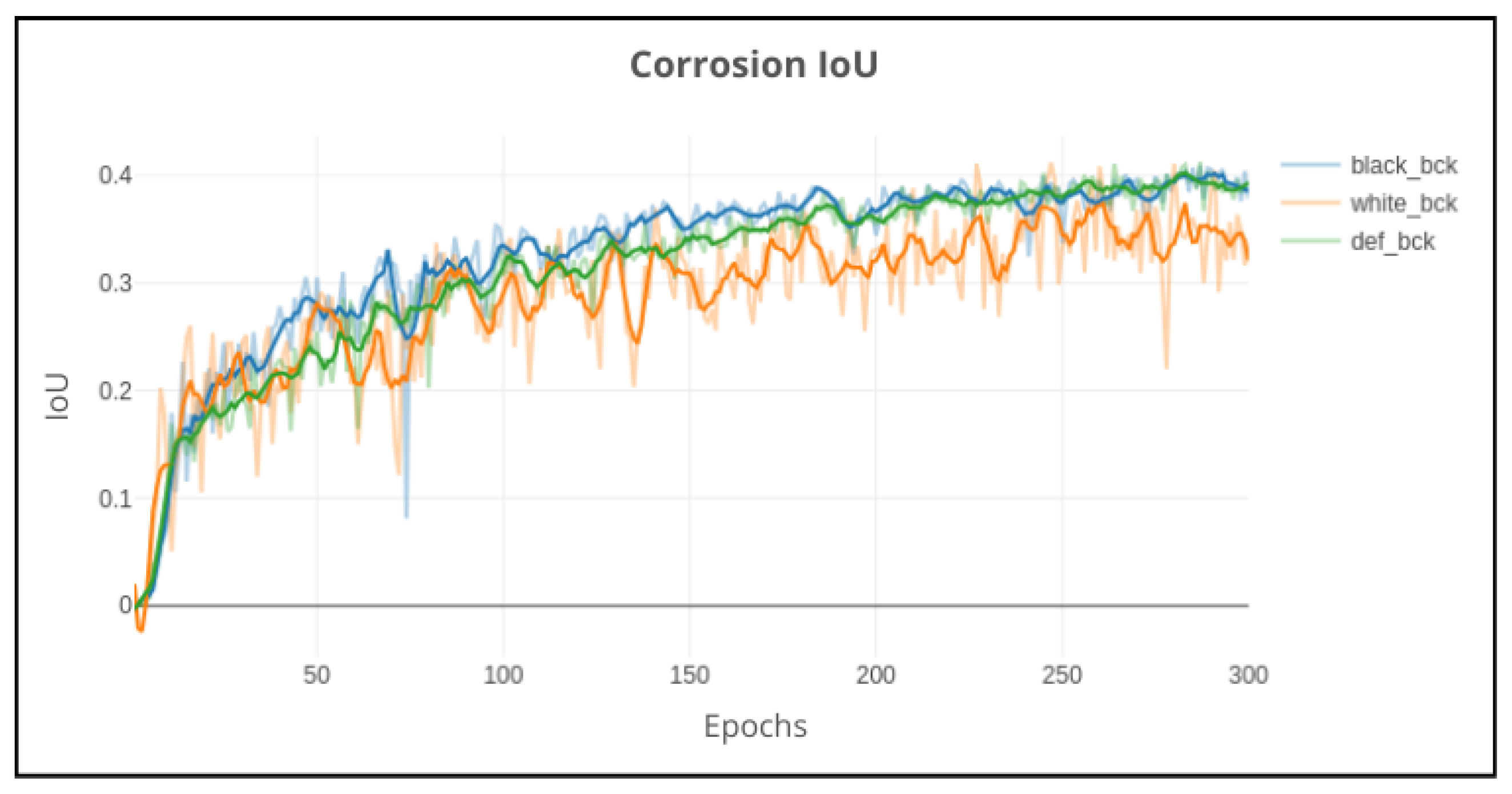
Figure 19.
DeepLabv3+: Impact on validation performance with or without data augmentation on 300 epochs.
Figure 19.
DeepLabv3+: Impact on validation performance with or without data augmentation on 300 epochs.
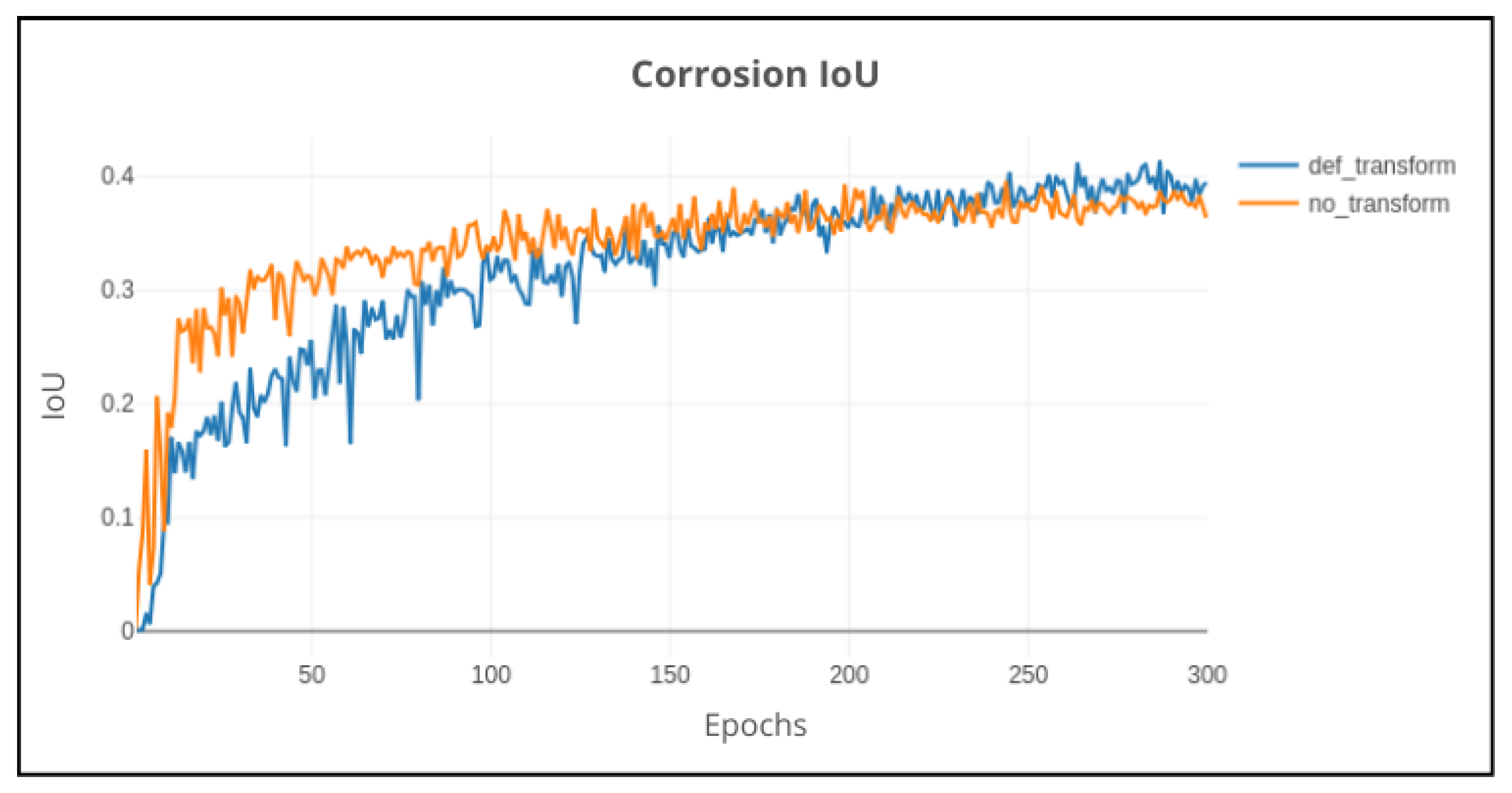
Figure 20.
DeepLabv3+ (smoothed lines): Impact on validation performance using MobileNetv2, Resnet50 and Resnet101 backbone network models on 300 epochs.
Figure 20.
DeepLabv3+ (smoothed lines): Impact on validation performance using MobileNetv2, Resnet50 and Resnet101 backbone network models on 300 epochs.
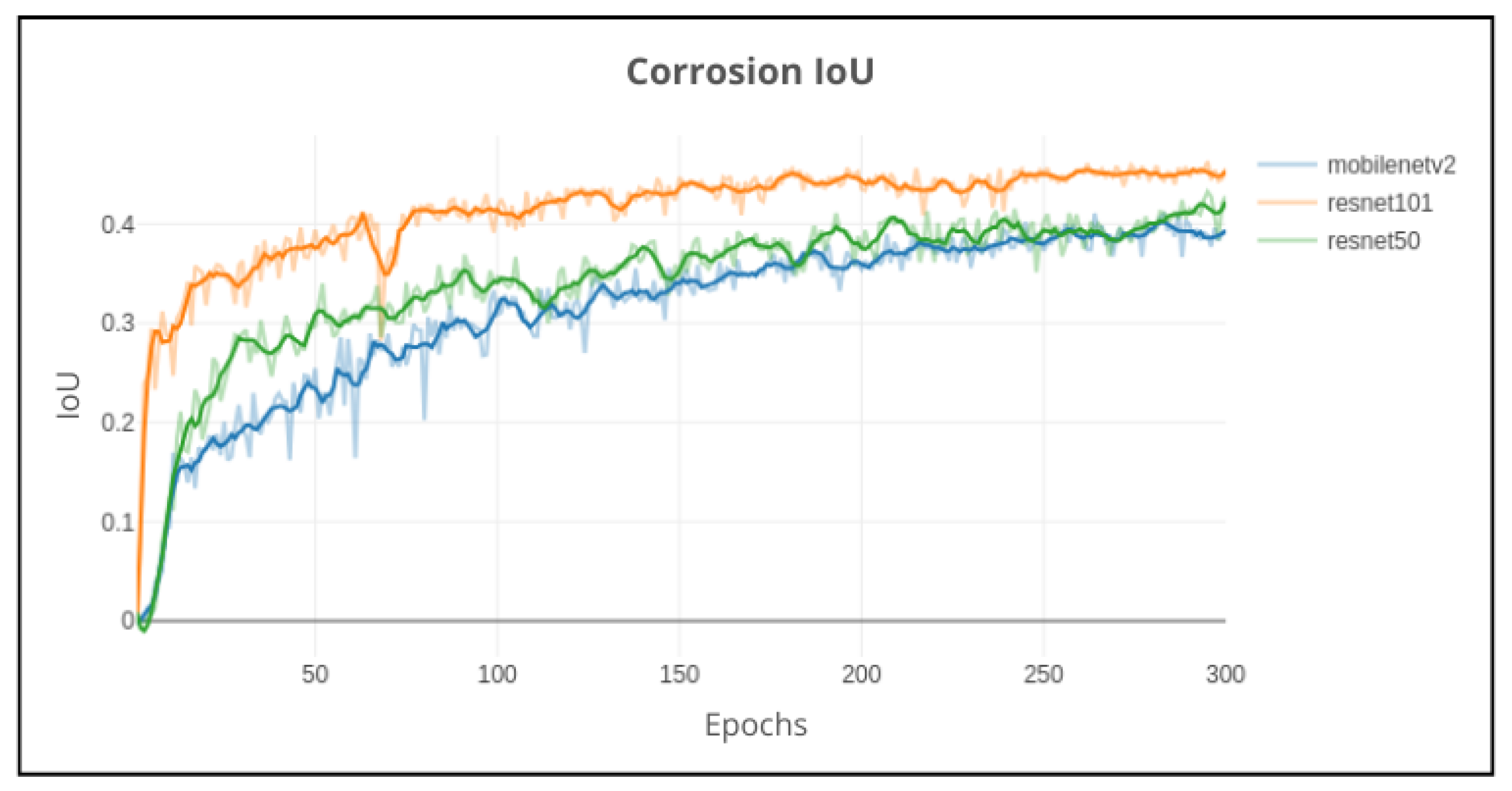
Figure 21.
DeepLabv3+ (smoothed lines): Impact on validation performance using SGD (300 epochs), Adam and AdamW on 200 epochs.
Figure 21.
DeepLabv3+ (smoothed lines): Impact on validation performance using SGD (300 epochs), Adam and AdamW on 200 epochs.
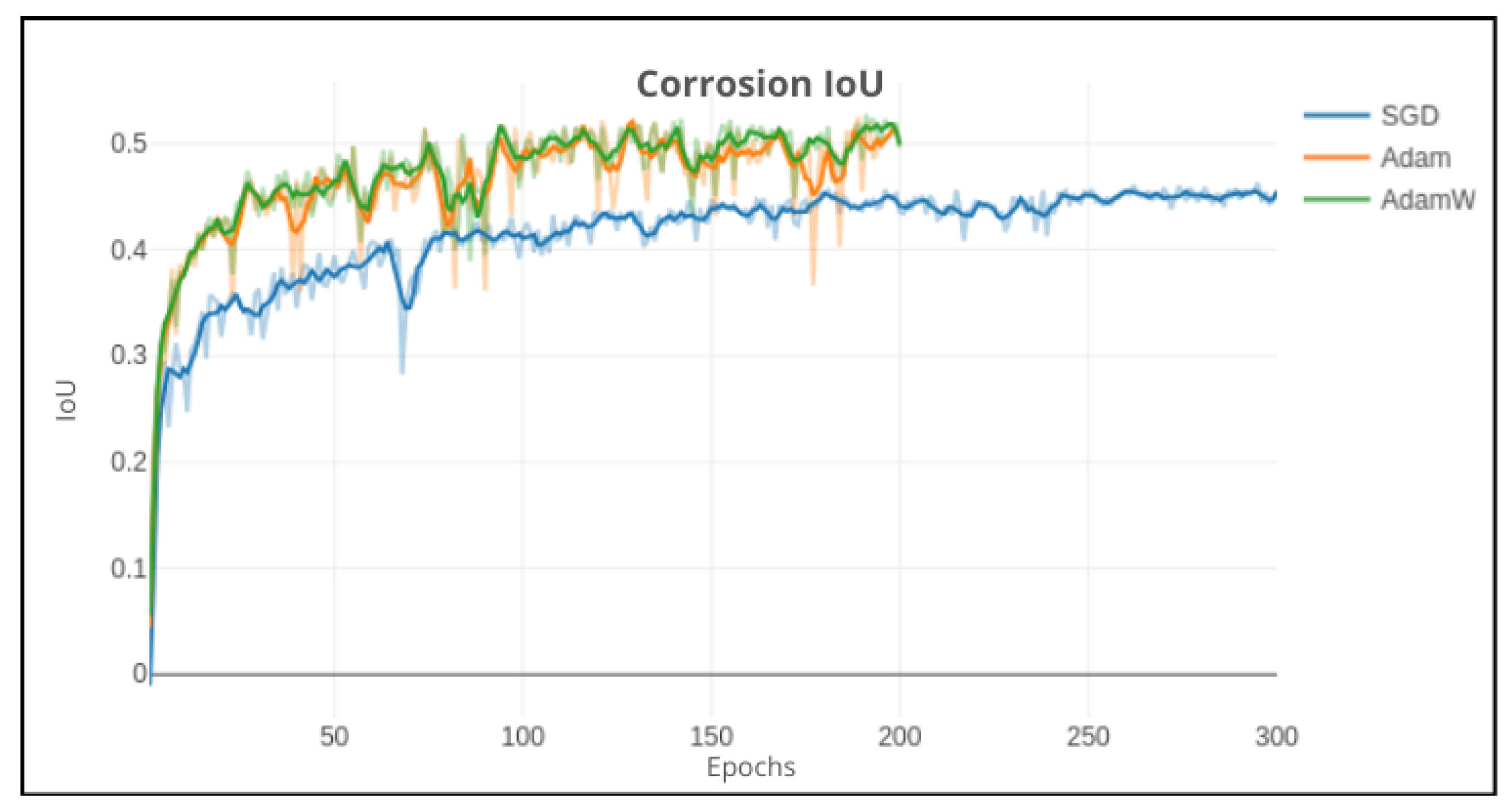
Figure 22.
Validation: Comparison of the output prediction with the ground truth mask and the original image.
Figure 22.
Validation: Comparison of the output prediction with the ground truth mask and the original image.
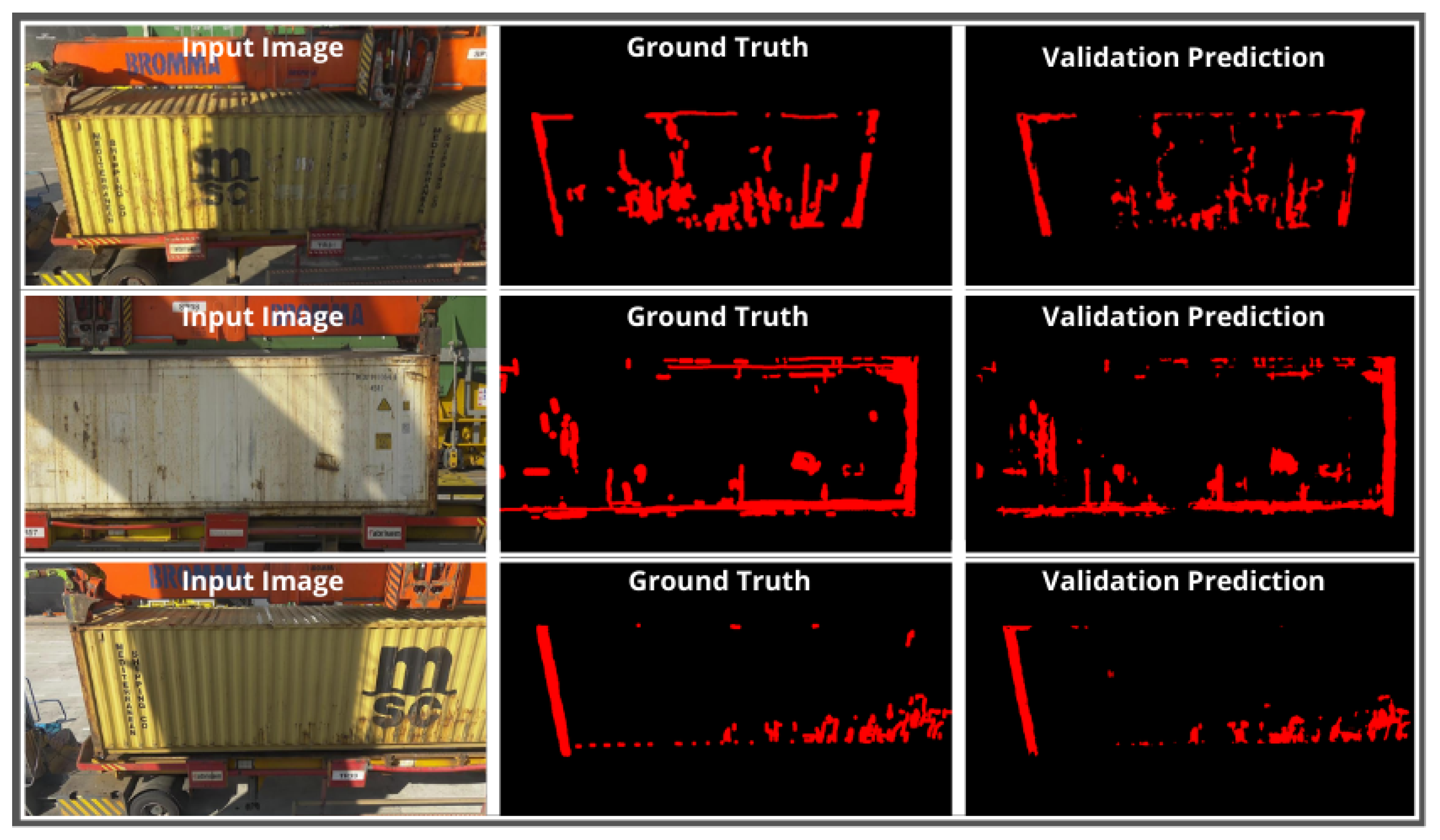
Figure 23.
Test: Comparison of the output prediction with the ground truth mask and the original image.
Figure 23.
Test: Comparison of the output prediction with the ground truth mask and the original image.

Figure 24.
Validation mean IoU using ResNet101 and AdamW (lr = 0.002) on 200 epochs.
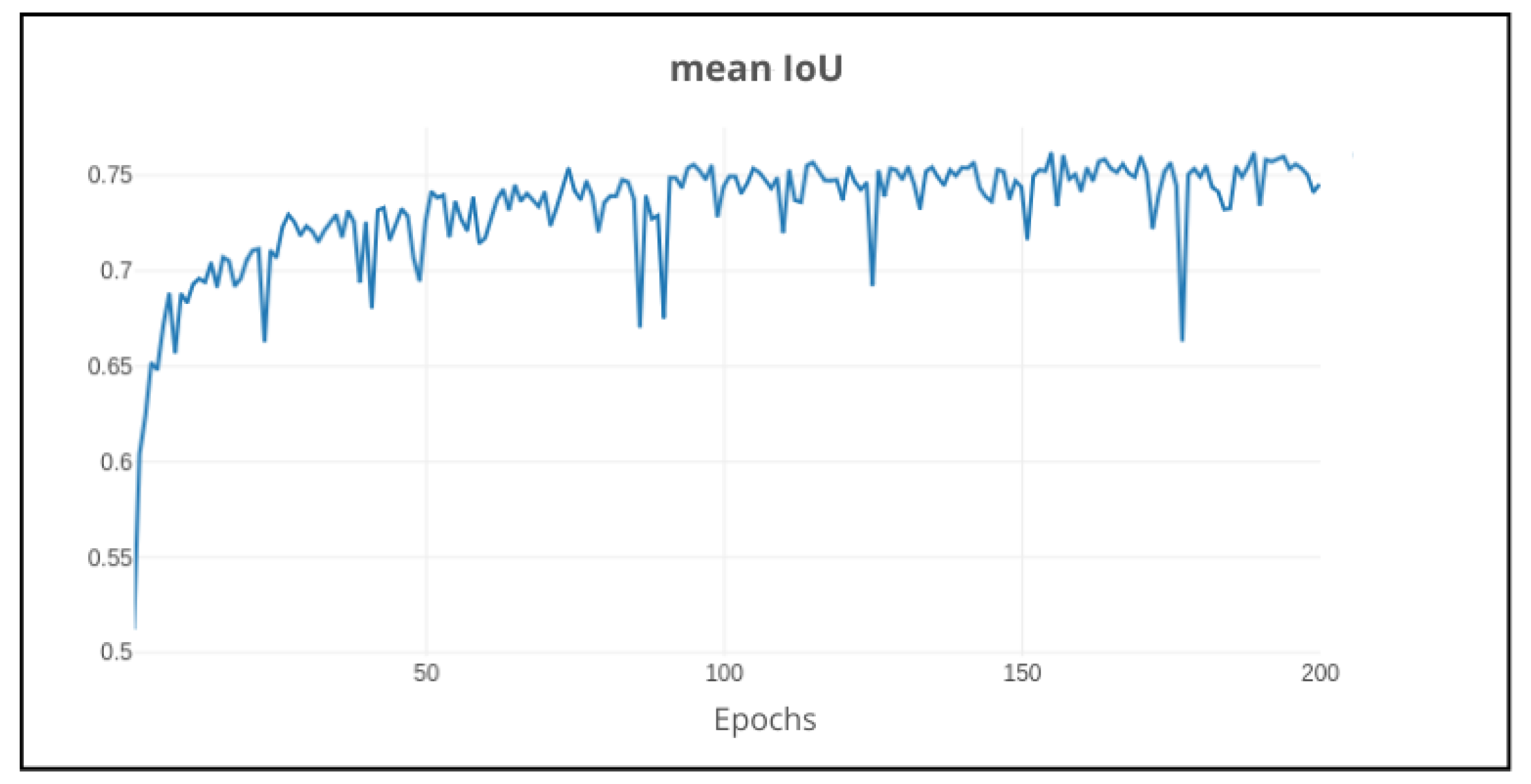

Table 1.
Number of canny edge pixels and laplacian values.
| Image | Canny Edges | Laplacian Variance |
|---|---|---|
| Rejected 1 | ≈ 77,000 | 11 |
| Rejected 2 | ≈ 42,000 | 11 |
| Rejected 3 | ≈ 6,000 | 2 |
| Rejected 4 | ≈ 5,500 | 3 |
| Acceptable 1 | ≈ 316,000 | 54 |
| Acceptable 2 | ≈ 129,000 | 23 |
| Acceptable 3 | ≈ 137,000 | 85 |
| Acceptable 4 | ≈ 318,000 | 50 |
Table 2.
Comparison of generic tools
| Tool | Open Source | Friendly UI | Large-scale Datasets | Pixel-Level Labeling |
|---|---|---|---|---|
| CVAT | ✓ | ✓ | ✓ | ✓ |
| LabelStudio | ✓ | ✗ | ✓ | ✓ |
| LabelBox | ✓ | ✗ | ✓ | ✓ |
| VIA | ✓ | ✓ | ✗ | ✗ |
| LabelMe | ✓ | ✓ | ✗ | ✗ |
Table 3.
Comparison of CV annotation tools
| Tool | Brush Tool | AI Magic Wand | Intelligent Scissors | Bounding Box | Points |
|---|---|---|---|---|---|
| CVAT | ✓ | ✓ | ✓ | ✓ | ✓ |
| LabelStudio | ✓ | ✓ | ✓ | ✓ | ✓ |
| LabelBox | ✓ | ✓ | ✓ | ✓ | ✓ |
| VIA | ✗ | ✗ | ✗ | ✓ | ✓ |
| LabelMe | ✗ | ✗ | ✗ | ✓ | ✓ |
Table 4.
Resampling filters comparison of downscaling and upscaling [22].
Table 4.
Resampling filters comparison of downscaling and upscaling [22].
| Resampling Filter | Downscaling quality | Upscaling quality |
|---|---|---|
| NEAREST | ||
| BOX | ★ | |
| BILINEAR | ★ | ★ |
| HAMMING | ★★ | |
| BICUBIC | ★★★ | ★★★ |
| LANCZOS | ★★★★ | ★★★★ |
| Model | PASCAL VOC (mIoU %) | Cityscapes (mIoU %) |
|---|---|---|
| FCN | 62.2 | 65.3 |
| SegNet | - | 57.0 |
| PSPNet | 82.6 | 78.4 |
| DeepLabV3 | 85.7 | 81.3 |
| DeepLabV3+ | 87.8 | - |
Table 6.
DeepLabv3+ pre-trained performance (IoU) on experiments 1 (20 random images), 2 (40 images without red cargo containers) and 3 (20 images with only red cargo containers). The experiments were tested on all different model weights with each respective loss function: w18 (cross entropy), w27 (l1 loss), w35 (l2 loss), w40 (cross entropy with weighted classes). Comparison of model performance in original image against white and black backgrounds.
| Experiments | Weights | Original | White Background | Black Background |
|---|---|---|---|---|
| 1 | 18 | 9.3% | 14.5% | 16.3% |
| 27 | 15.5% | 20.4% | 21.1% | |
| 35 | 14.9% | 18.7% | 18.9% | |
| 40 | 10.3% | 22.0% | 20.5% | |
| 2 | 18 | 6.9% | 13.1% | 14.9% |
| 27 | 12.2% | 17.7% | 18.5% | |
| 35 | 9.2% | 14.4% | 14.9% | |
| 40 | 9.3% | 18.3% | 14.8% | |
| 3 | 18 | 0.6% | 1.4% | 1.6% |
| 27 | 0.9% | 2.4% | 1.9% | |
| 35 | 1.0% | 1.5% | 1.5% | |
| 40 | 0.8% | 0.9% | 1.7% |
Table 7.
DeepLabv3+ fine-tuned performance (IoU) on validation set and test set for each configuration in all experiments.
Table 7.
DeepLabv3+ fine-tuned performance (IoU) on validation set and test set for each configuration in all experiments.
| Experiments | Configuration | Validation | Test |
|---|---|---|---|
| Background | Default | 41.3% | 30.0% |
| Black | 40.1% | 30.4% | |
| White | 41.0% | 29.5% | |
| Data Augmentation | Default | 41.3% | 30.0% |
| Without | 39.4% | 29.3% | |
| Networks | MobileNetV2 (def) | 41.3% | 30.0% |
| ResNet50 | 43.2% | 34.7% | |
| ResNet101 | 46.3% | 40.1% | |
| Optimizers | SGD (def) | 46.3% | 40.1% |
| Adam | 52.5% | 49.4% | |
| AdamW | 52.7% | 49.4% |
Table 8.
Performance comparison of DeepLabv3+ pre-trained model with fine-tuned model.
| DeepLabv3+ Model | Performance (IoU) |
|---|---|
| Pre-trained | 4.0% |
| Fine-tuned | 49.4% |
Disclaimer/Publisher’s Note: The statements, opinions and data contained in all publications are solely those of the individual author(s) and contributor(s) and not of MDPI and/or the editor(s). MDPI and/or the editor(s) disclaim responsibility for any injury to people or property resulting from any ideas, methods, instructions or products referred to in the content. |
© 2025 by the authors. Licensee MDPI, Basel, Switzerland. This article is an open access article distributed under the terms and conditions of the Creative Commons Attribution (CC BY) license (http://creativecommons.org/licenses/by/4.0/).
Copyright: This open access article is published under a Creative Commons CC BY 4.0 license, which permit the free download, distribution, and reuse, provided that the author and preprint are cited in any reuse.


