

Submitted:
10 April 2025
Posted:
12 April 2025
You are already at the latest version
Abstract
In this work we present a numerical approach for solving optimal control problems for fluid heat transfer applications with an emphasis on the coupling of multiple codes. Specifically, two different CFD codes, OpenFOAM (finite volume based) and FEMuS (finite element based), have been used to solve the optimality system, while the data transfer between them is managed by the external library MEDCOUPLING. The state equations are solved in the finite volume code, while the adjoint and the control are solved in the finite element one. Two examples taken from the literature are implemented in order to validate the numerical algorithm: the first one considers a natural convection cavity resulting from a Rayleigh-Bénard configuration, and the second one is a Conjugate Heat Transfer problem between a fluid and a solid region.
Keywords:
Boussinesq approximation
; Conjugate Heat Transfer
; natural convection
; optimal control
; code coupling
1. Introduction
One of the most important aspects in the design of an engineering system is foreseeing the physical behavior of the variables considered. Knowing the range in which a specific quantity can evolve is a crucial issue in checking the correct operation of a given apparatus. In this context, the numerical simulation of the partial differential equations that describe physical phenomena turns out to be essential. Specifically, the standard approach for a numerical simulation consists of building a parameter set, such as boundary conditions, source terms, and material physical properties that, given as an input to the conservation equations, provides a numerical output that describes the evolution of the physical system. On the other hand, this approach leads to a try-and-fail approach since we do not have direct control over the output results, and thus it can become expensive from a computational point of view. However, numerical optimization is proposed as a viable alternative to the former approach because the desired outputs turn into input parameters that can be selected in the model. In fact, the idea is to minimize a cost function that represents the distance between a variable and its desired target value under specific physical constraints that are the governing equations [1]. We can therefore introduce the objective term that represents a physical quantity to be obtained, such as a velocity or temperature matching, but also the enhancement or the reduction of a specific variable. The control term is a physical parameter that is used to perform the minimization, and it can be distributed over the domain, or it can act only on the boundaries. Possibly, the control can modify the geometry of the problem in the context of shape optimization [2]. Lastly, objective and control terms must follow the governing equations that have the role of constraints describing the physics under investigation.
In this work, we present a numerical optimization algorithm that considers generic heat transfer problems. In particular, we present two examples that are representative of physical phenomena commonly present in several engineering applications. The first one involves the solution of the Navier-Stokes and energy equations (under the Boussinesq approximation) in the context of a natural convection problem considering the Rayleigh-Bénard setting as described in [3]. The second one is described by the Conjugate Heat Transfer (CHT) model, which describes the heat transfer between a solid and a fluid region as seen in [4]. Specifically, we adopt an adjoint-based optimization, which entails the solution of a coupled system given by the state, adjoint, and control equations [5].
Regarding the first application, several results have already been shown in the literature. One of the first works appears in [6], where a natural convection optimal control problem has been considered for a two-dimensional square cavity and for a temperature matching problem. In [7], an optimal control problem for the Boussinesq system has been presented in the context of liquid metals in a differentially heated cavity, while in [8] the same approach is described with the addition of a dynamic turbulence model. Several papers have shown the existence, uniqueness, and regularity of the solution for this kind of problem. The interested reader can consult [9,10,11,12,13,14,15,16,17,18,19,20], where different settings are taken into account, including the use of different control approaches. For the specific problem of the boundary control problem considering the stationary Rayleigh-Bénard-Marangoni setting, one can consult [21]. Regarding the optimal control of the heat transfer between a fluid and solid region, or more in general heat transfer problems, we refer to [4,22,23].
Nevertheless, validated and state-of-the-art codes already exist nowadays, at least for the state equations (i.e. the constraints of the optimal control system). Therefore, the aim of this paper is to leverage these codes to build the optimal control system. Here we extend the work presented in [24,25] with the aim of coupling two CFD codes for the implementation of a heat transfer optimal control problem. The idea is to use the finite volume (FV) code OpenFOAM [26] for the solution of the state equation and the in-house finite element (FE) code FEMuS [27] for the adjoint and control equations. In fact, the latter equations arise naturally from a variational formulation of the considered problem, justifying the use of a finite element approach. In this framework, the latter equations should be solved because their derivation requires the concept of variation of the unknowns, with the possibility of also including the gradient of the variations. It appears clear from a mathematical point of view that the finite element approach lends itself to these representations which are often missing or cumbersome to evaluate in standard finite volume frameworks. The code coupling, i.e. the data transfer between the different codes, is implemented by using the external library MEDCOUPLING [28].
Additionally, two main approaches can be followed when dealing with optimal control problems. The first one consists of discretizing the optimality systems after minimizing the functional considering an infinite-dimensional framework (Optimize then discretize). Differently, the second one discretizes the Lagrangian equation, and then it derives the different equations to be solved (Discretize then optimize). Under generic assumptions, these two approaches do not produce the same set of equations [1,5]. The numerical code coupling by using finite volume and finite element discretization can implement only the first approach, since with the second one, the discretized equations, such as the adjoint and the control, follow directly from the discretization used for the Lagrangian function.
The paper is organized as follows: in the first section, we derive the optimality systems for the heat transfer problems, one considering the Boussinesq equations, and a second one for the Conjugate Heat Transfer between solid and fluid. After that, we provide a brief description of the numerical algorithm for the code coupling involving the two CFD codes via the external library. Lastly, we provide two numerical examples in order to validate the proposed numerical approach considering numerical benchmarks taken from the literature.
2. Optimal Control Problems
In this section, we present and describe the mathematical formulation of the system of equations considered for both numerical problems. We start by considering the state equations that indeed describe the different methods to transfer heat, i.e., the Boussinesq system and the Conjugate Heat Transfer. After that, since the examples involve different objective and control terms, we derive each optimality system considering the specific application setup.
We first introduce some mathematical notation from functional analysis [29]. Considering a generic domain , denotes the standard Sobolev space of order , and clearly the space of square-integrable functions refers to the zero-order Sobolev space ,
Of particular interest is the space defined as
and we also introduce the subspace of functions that vanish on the boundary ,
For a generic element f of the Sobolev spaces, the norms can be written as
and
where . For functions defined only on the boundary of the domain , then its norm is defined as
where the surface gradient is . Lastly, for such that , where is the Sobolev space of integrable functions , their inner product is defined as
In the case of vector-valued spaces, we indicate them with boldface letters . Their norm is defined in a completely analogous manner to the scalar case. Taking , the inner product is defined as
Next, we introduce the bilinear forms
and the trilinear forms
that will be useful in the description of the optimality systems.
We introduce the functional that we define as
where represents the generic objective functional, i.e. or , and the regularization term with for distributed control and or for boundary control. In this paper, we will address Dirichlet boundary control problems with regularization while Neumann boundary control problems with regularization. In both cases we are restricting the space where we are looking for the solution with respect to its native space, respectively and . For more details regarding this aspect and the different numerical approaches to address this issue, the interested reader can consult [30,31,32,33].
2.1. Rayleigh-Bénard Problem
In this section, we derive the optimality system for the Rayleigh-Bénard problem considering a square domain as reported in Figure 1. The Rayleigh-Bénard system exhibits buoyancy-driven flow, where the natural convection develops due to the temperature gradient imposed between the two horizontal walls and . The objective of this optimization case is to stabilize the flow inside the domain, thereby minimizing the vorticity. This will be achieved by introducing appropriate cavity heating, initially using a volumetric heat source within the domain, and then applying a heat flux condition on the boundary.
The coupled Navier-Stokes system and energy equation form the Boussinesq system of equations that model the Rayleigh-Bénard problem. We write the stationary form of the Navier-Stokes equations as
where is the velocity field, p is the pressure field, is the kinematic viscosity, is the thermal expansion coefficient, is a vector representing the gravitational acceleration in the negative y direction, and is the rate of deformation tensor of the flow. Next, we write the stationary energy equation in the temperature formulation as
where T is the temperature field, Q is a generic volumetric heat source, is a generic wall heat flux, is a given temperature profile ad the boundary and is the thermal diffusivity coefficient. The temperature gradient inside the cavity is generated by fixing the temperature along the top wall and part of the bottom wall according to . As mentioned earlier, the vorticity minimization is achieved by controlling the volumetric heat source Q and the wall heat flux separately, however, the generic derivation for both types of control is reported below.
The weak formulation of the state constraints (1) and (2) is written using the linear, bilinear, and trilinear forms introduced earlier
Then we specialize the generic functional to this case, i.e.
where are the regularization coefficients for the distributed and the Neumann boundary control cases. Note that, in the case of boundary control, since we are dealing with the temperature derivative, the regularization is intended to be in . We also introduce the Lagrange multipliers , referred to as the adjoint variables, corresponding to the adjoint velocity, adjoint pressure, and adjoint temperature, respectively. Finally, we write the Lagrangian as
Taking the variational derivative of the Lagrangian in the adjoint directions, we re-obtain the state equation system (3). Then we take the variation of the Lagrangian in the state directions , obtaining the adjoint equation system
Finally, we differentiate the Lagrangian in the two control variables direction
clearly taking we solve the distributed control case, while taking we solve the boundary control case. From these two equations, we can derive the functional gradient used in the steepest descent method as
respectively.
Finally, we write the strong form of the optimality system. We must isolate the velocity variation to achieve this. To do so, we perform the following integrations by parts
Considering both the divergence of the velocity and the adjoint velocity on the boundary to be zero, we obtain the following strong form for the adjoint velocity system of equations, which corresponds with the steady formulation of the Oseen equation [34]
Isolating the temperature variation in the adjoint system (6) after some manipulation
where in the second one we used the divergence-free property of . Since the temperature variation vanishes on the boundary due to the Dirichlet condition on T, we obtain the following strong form system for the adjoint temperature
Lastly, the strong form of the control equations, both for the distributed and the boundary control case, is obtained directly from equations (7) leading to
2.2. Solid/Fluid Heat Transfer Problem
In this section, we derive the optimality system for the solid-fluid domain depicted in Figure 2. Moreover, during the following derivation, we will include some additional steps compared to the previous case for the sake of clarity. Unlike the previous case, the system here is considered to operate in a forced convection regime. As a result, the buoyancy term in the Navier-Stokes equations can be neglected. Furthermore, we impose a controlled inlet flow on the boundary and an outflow condition on . The corresponding system of equations reads
where the stress tensor is defined as , and is the kinematic viscosity for the fluid. The temperature is solved both in the solid and the fluid domain, and on the interface, a conjugate heat transfer condition is imposed. In the following, we define a CHT interface condition as the condition of continuity of temperature as well as normal heat flux. We fix the temperature on while we consider the other walls to be insulated. Furthermore, in the solid region, a volumetric heat source Q is enforced. We write separately the system of equations for the solid region
and for the fluid region
where and are the thermal diffusivity coefficients for the solid and fluid regions, respectively.
Now, we derive the weak form of the Navier-Stokes system after performing the following steps:
While in the Boussinesq case both boundary terms were zero due to the choice of the test function , in this application they give a contribution on . Then, we can write the weak formulation for the Navier-Stokes equations system as follows
where the Dirichlet boundary condition at the inlet is also formulated weakly in order to obtain the control in the desired function space. For the temperature system, we first integrate the Laplacian term in the solid and the fluid systems to get
After summation of the above equations, the two boundary terms on cancel each other due to the heat flux continuity. Then, we can write the temperature equation for the whole domain in weak form as
where of course the diffusivity constant is being H the Heaviside function.
Now we introduce the cost functional
where is the observation boundary and an regularization is chosen since we deal with a Dirichlet boundary control [35]. Even if we use two different weights, and , the existence of the solution for a Dirichlet boundary optimal control necessarily requires the regularization of the gradient term if we consider a CHT problem [4,36], i.e. . Using again the Lagrange multipliers , we write the Lagrangian as
Taking the variational derivative of the Lagrangian in the adjoint direction, we re-obtain the state equations (17) and (18). In order to derive the adjoint velocity system, we differentiate in the velocity and pressure p direction to get
Similarly, by taking the variation of the Lagrangian in the temperature T direction, we obtain the weak form of the adjoint temperature equation
Lastly, differentiating the Lagrangian with respect to the control variable we obtain the Euler equation in weak form
In order to iteratively solve this system through the gradient descent method, we need the explicit formulation for the Lagrangian derivative in the control direction, which clearly results in
Once again, we transition from the weak form of the adjoint velocity system to the strong form. Specifically, we start isolating the velocity variation . To do so, we perform the same steps reported in (9), i.e. we perform some manipulations to obtain
Taking the velocity variation to vanish on and due to Dirichlet conditions, and the adjoint velocity to vanish on , , as shown in the weak formulation of the system, we obtain the following strong form for the adjoint velocity system of equations
Performing the same steps as in (11), we write the strong form equation system for the adjoint temperature as
Lastly, the strong form of the control equation is easy to obtain directly from equation (23)
2.3. Minimization Method
The optimality system consists of the state equations for , the adjoint equations for , and the control equation, or optimality condition, for , and . These three systems of equations are clearly coupled but are solved in a segregated manner, as mentioned, to reduce computational effort. The state and adjoint systems are solved using a simple fixed-point iteration method, while for the control variables, to ensure convergence to the optimum, we employ a basic gradient method with a backtracking line search algorithm, as shown in Algorithm 1. Here we refer to the control variable with the generic symbol q. It can be demonstrated that, for a sufficiently small step size that the backtracking line search algorithm always guarantees, the gradient method yields descent direction and is globally convergent [37]. As mentioned, the control update in line 8 is performed using a gradient method. Firstly, the control variation in the three different cases is calculated as
and then the update is performed
| Algorithm 1:Steepest gradient method |
|
3. Coupling Algorithm
In this section, we present the numerical algorithm for the code coupling that solves the state equations separately from the adjoint and control equations. The previous section has given a detailed explanation on the reasoning to adopt a finite element framework for solving the adjoint and control equations. Moreover, the coupling application leverages the well-validated OpenFOAM solvers, making it a reliable tool for solving the state equations and eliminating the need for re-implementing traditional conservation equations.
Data exchange between the two codes has been made possible by implementing three C++ classes. The first class, med_coupling, manages the data transfer routines with the external library MEDCOUPLING, specifically for data manipulation and interpolation. Furthermore, we have two specific wrapper classes for the CFD codes. The first one, referred to as of_interface, is responsible for the communication between the routines of OpenFOAM and the MED data structure. The corresponding class for the FEMuS code is labeled as femus_interface. More details regarding the specific implemented classes and the coupling strategy can be found in [24]. With the previously described code architecture, we describe the specific algorithms for the Rayleigh-Bénard problem and the solid/fluid heat transfer problem in the following sections.
3.1. Rayleigh-Bénard Problem
For the first application, we want to couple FEMuS and OpenFOAM in order to solve a Rayleigh-Bénard problem describing the natural convection inside a cavity. The state equations to be solved are the Navier-Stokes equations in the incompressible formulation together with the temperature equation, as described in the previous section. This system of equations is then solved by adding the adjoint and the control equations, which can be both a volumetric source or a boundary condition for the temperature equation. In this work, we present these two different data type transfers, i.e. a volumetric and a boundary approach. For more details regarding the data transfer with the external library MEDCOUPLING, the interested reader can consult [24], where each routine used in this work is explained.
The data exchange from OpenFOAM to FEMuS involves transferring the state variables: the velocity and the temperature T fields. Thus, the get and set functions extract these volumetric fields from OpenFOAM and write them into FEMuS for the solution of the adjoint equations. Note that this data exchange implies a transfer from a finite volume representation to a finite element data structure. The same approach applies to the control variable q, where the get and set functions transfer this variable from FEMuS to OpenFOAM. This data exchange can be used in both volumetric and boundary-based methods, with data interpolation now originating from a finite element grid and converting data to a finite volume grid. For the volumetric data transfer, q is the volumetric source of the temperature equation, while for boundary control, q is transferred to the Neumann boundary condition of the same equation. A schematic representation of this algorithm is reported in Figure 3.
3.2. Solid/Fluid Heat Transfer Problem
For this test, we exploit already validated numerical tools available in OpenFOAM for the solution of the state equations. In particular, we refer to the multi-region technique, which provides tools to exchange data between two regions, such as the conjugate heat transfer approach.
The schematic representation for the application is reported in Figure 4. The data transfer between the CFD codes follows the same volumetric and boundary data exchange described in the previous application. However, the of_interface class has been improved to support the multi-region solver of OpenFOAM, allowing for the retrieval of field values within different domains. In this application, the temperature field is transferred from OpenFOAM to FEMuS not only across the entire fluid domain but also at the interface between the two regions. Moreover, OpenFOAM supplies the volumetric velocity field to FEMuS, while FEMuS provides the boundary control q to the fluid domain in OpenFOAM.
It is worth noting that OpenFOAM exploits a segregated approach in the implementation of the CHT boundary condition between the solid and the fluid, i.e. the two regions are solved separately, and then the boundary conditions are enforced on , taking into account the continuity of the temperature field and the conservation of the heat fluxes. On the other hand, FEMuS solves the adjoint temperature in a monolithic way on a single domain which includes both the solid and the fluid region. Therefore, we do not enforce additional boundary conditions on the common interface since the assembling of a unique matrix allows us to satisfy the continuity conditions on temperature and heat flux in a natural way. Of course, different material properties and source terms are taken into account depending on the specific domain where the local element of the mesh is assembled.
Lastly, we remark that OpenFOAM solves the Navier-Stokes system only by a projection method, and we selected the PIMPLE algorithm. On the other hand, a monolithic approach is implemented in FEMuS for the adjoint Navier-Stokes, which indeed couples the adjoint velocity and pressure by assembling and solving them simultaneously.
3.3. Numerical Discretization
We briefly discuss the discretization framework of the equations. We already know that the state equations are solved with a finite volume approach while the adjoint and control equations use a finite element discretization. In the introduction, we also mentioned the use of the optimize then discretize concept to build our optimal control problem that supports different discretization spaces for the approximation of the state and adjoint equations. We introduce the finite dimensional spaces , and . Specifically, given a domain partition , the element K, and the space of polynomials of degree at most r, we set
We refer to the vector-valued version of the same spaces with a bold symbol. Regarding the discretized adjoint variables, we consider a standard Taylor-Hood pair for the adjoint velocity and pressure [38,39], thus we have . For the adjoint temperature and the control, we consider biquadratic finite elements, i.e. .
The finite volume approximation of the state equations requires only one type of discretized space. Therefore, we consider the piecewise constant approximation for velocity, pressure and temperature, i.e. and .
4. Numerical Results
In this section, we present two numerical examples in order to validate the effectiveness of the above-presented algorithm. As a first numerical test, a Rayleigh-Bénard natural convection problem is described considering a square cavity. Later, we present a multi-region problem with a solid and a fluid domain that interact via a standard conjugate heat transfer model. For each application, we recall the objective functional, the control term in the state equations, and the corresponding boundary conditions. Numerical results are then compared with already published works with the same problem setting.
4.1. Rayleigh-Bénard Problem
For the first numerical test, we refer to the example reported by Lee [3], where a vorticity minimization has been studied on a square domain. Specifically, the natural convection obtained from the Rayleigh-Bénard configuration has been simulated with both a distributed and a Neumann boundary control for the temperature equation. Among the several cases reported in [3], we selected two of them that present different behaviors of the control and the optimal solution. Therefore, after a comparison of the uncontrolled solution, the cases with and will be discussed (same values have also been considered for the Neumann case, i.e. for ).
In Figure 5, the domain is shown, with the partition of the bottom boundary into two sections, and . The boundary conditions for the temperature field are as follows: a homogeneous Neumann is enforced on and ; on we have a homogeneous Dirichlet boundary condition, while on we have a fixed temperature value . Lastly, on we have the nonhomogeneous Neumann boundary condition that acts as control.
The grid used for the simulation consists of elements for the FE code and elements for the FV code, both equally spaced. This discretization setup leads to a very similar amount of degrees of freedom for each code (the finite element grid is indeed equipped with biquadratic elements, therefore implying 1681 dofs).
In the case of the distributed control, we fix , while for the Neumann boundary control we set . Regarding the material properties of the fluid, we set .
We recall the optimality system in strong form for this problem, given by (28), (29) and (34), along with the corresponding boundary conditions reported in Table 1.
4.1.1. Uncontrolled Case
The results for the uncontrolled case (namely, the control variable is set to zero) are shown in Figure 6. The contour plot of the temperature field is shown on the left side, while the velocity field is shown on the right.
4.1.2. Distributed Control
Figure 7 shows the results for the temperature fields in the distributed control case, compared to the same contour plot from [3] which is shown with a dashed line. We observe that both temperature distributions get closer and closer to a purely vertical temperature gradient. It appears that the reduction in the horizontal temperature gradient leads to a temperature profile and hence a buoyancy force that is nearly constant along a single horizontal line. This evens out the horizontal differences in buoyancy and contributes to the minimization of the vorticity. A good agreement with respect to the reference paper can be observed for the isolines of the temperature field, in particular for the lowest value.
The contour plot of the control Q is shown in Figure 8, on the left for the case with and on the right for . We recall that the control Q acts as the volumetric source of the temperature equation, and we can see the different distributions for the two values of . The lower the regularization factor , the more the Q field concentrates in magnitude at the bottom of the domain.
Figure 9 shows the adjoint velocity vector glyphs for each controlled case.
Similarly, Figure 10 shows the velocity vector glyphs for each controlled case. Note that in this case we have rescaled the velocity profiles by a common scalar, in order to visualize the overall reduction in magnitude.
Specifically, the computed values of are reported in Table 2, where it can be noticed that the velocity magnitude decreases by increasing the control contribution, i.e. with a lower value.
In Table 3, we report the value of the objective term, the regularization term, and the total functional for the distributed case, with a comparison to the same results from [3]. In the last column, we have reported the relative error of the total functional, computed as
where the subscripts C and R stand for Coupled and Reference, respectively. For the same reason, the results presented in this work are labeled with C in the table. As we can see, the proposed algorithm is able to reproduce the same values of the cost functional terms with an error below , validating the accuracy of the numerical code coupling. A good agreement is evident in each of the above cases. Slight differences appear for the uncontrolled case, while the results of the code coupling algorithm become closer and closer to the literature ones by decreasing the control parameter .
4.1.3. Neumann Boundary Control
Regarding the Neumann boundary control, in Figure 11 we plot the control along the boundary for each controlled case ( and ). In this case, this control represents the Neumann boundary condition for the temperature equation, which can be understood as the wall heat flux provided in order to minimize the vorticity. For the highest case the control seems to grow monotonically, while for we can notice a peak in the left part of , which is attached to where we have a fixed temperature boundary condition. We remark that on the point between and the adjoint temperature is zero. Hence, cannot help pushing the control at this point and so the control tends to have a local maximum nearby in order to compensate for the lack of push.
In Figure 12, the contour plot for the temperature is reported for the Neumann boundary control case for each , together with the reference case [3] represented by dashed lines.
Some discrepancies appear between the solid isolines and the corresponding dotted lines as reported in [3], especially for the case in the bottom part of the domain, where indeed we have the control . This situation improves with the lower .
The velocity fields are reported in Figure 13 for both controlled cases. Moreover, in Table 4 we report a comparison of the maximum value of the velocity magnitude for the computed cases, and we notice a difference of one order of magnitude between the results of the two values.
4.2. Solid/Fluid Heat Transfer Problem
In the second test, we reproduce the numerical examples proposed in [4], which we use as a benchmark. Here a fluid domain exchanges heat with a neighboring solid region through a common boundary. This configuration is typically referred to as a conjugate heat transfer problem. The geometry is described in Figure 14, which shows two neighboring regions, for the solid and for the fluid. The boundary walls of the fluid domain are given by and , which is the common interface with the solid. On the walls a no-slip condition is enforced, i.e., a homogeneous Dirichlet boundary condition for the velocity field. On the other hand, and are the inlet and the outlet boundaries of the channel through which the fluid flows. We impose a Dirichlet boundary condition at the inlet and a stress-free condition at the outlet.
The boundaries of the solid domain are , , and . The boundary conditions for the solid region are given by a Neumann boundary condition for each external edge, while on the common interface we enforce the continuity of the temperature and of the heat flux between the two domains. The aforementioned benchmark case has been obtained within a finite element environment. This presents some challenges when transitioning to the finite volume method.
In the FE formulation, the point at the junction belongs to boundary sections that require a temperature Dirichlet condition on one side and a Neumann condition on the other. In the FE context with Lagrange shape functions, the point itself is a degree of freedom carrier, and the Dirichlet condition can be enforced in essential way.
On the other hand, in the FV framework, the degrees of freedom are given by the cell centers, and a Dirichlet boundary condition involves the face of an element. In this situation, the intersection point will not behave in the FV code in the same way as in the FE code. Therefore, the FE versus the FV solutions show a rather different behavior at this intersection point. We have observed with auxiliary numerical tests that the results in [4] have been obtained with a mesh size that yields a FE solution that is quite far from grid convergence. In spite of that, in order to compare with the reference paper values, we decided to choose an FV mesh with approximately the same dof count. At such a resolution, the Dirichlet value computed by the FV code on the lower-left corner of the solid domain turns out to be quite far from the FE value. We were able to fix this difference by simply enforcing a Dirichlet condition also on the first solid element above .
We use a element grid for the FE code and a similar-sized (from the d.o.f. point of view) cell grid for the FV code to replicate the results proposed in [4]. The latter grid is divided as a grid in the fluid region and a grid in the solid region, refined towards the solid/fluid interface . Concerning the thermal diffusivity, we have and , while the kinematic viscosity for the momentum equations is . Lastly, the volumetric heat source in the solid region is set .
We recall the optimality system in strong form for this problem, given by Eqs. (32), (33) and (34), along with the boundary conditions in Table 6:
Notice that the state equations are reported explicitly over the two regions since OpenFOAM solves in a segregated way, while the adjoint uses the monolithic formulation. We also remark that, as in [4], the Dirichlet condition on the inlet velocity is enforced only in the normal direction.
4.2.1. Definition of the Target Temperature
Following [4], the target of the control problem is the temperature profile on that is obtained with an analytical input velocity , i.e. a Poiseuille flow. In the following, we refer to this as the uncontrolled solution. The target is then fed to the optimal control system. For the solution of the optimality system, the first control in the steepest descent method is initialized with a different inlet boundary condition for the velocity field, i.e. , and therefore the control acts on the interface boundary to reach a velocity field that matches the temperature distribution as close as possible. It appears clear that the optimal solution should provide a control on the boundary that reproduces the original boundary inlet condition for the velocity field . In this way, it is easy to check the quality of the optimal control solution. Of course, due to the presence of a regularization term, i.e. a parameter , the control is not able to reproduce exactly that original velocity profile, but it provides the closest solution according to the value of .
In Figure 15, we report the target temperature solution. On the left we show the overall behavior as a contour map and on the right we plot the trend on a portion of the interface , which corresponds to the target temperature . We recall that the objective functional was defined only on a portion of the solid/fluid interface, i.e. the region . The isolines in the left figure confirm the interface conditions of the CHT model, i.e. the continuity of the temperature and the change in slope due to the continuity of the heat flux across different conductivities.
4.2.2. Dirichlet Boundary Control
In Figure 16, the Dirichlet velocity control on is reported as a solid line for two controlled cases. In particular in Case 1 we set the pair to , while in Case 2 we set . The comparison with the reference data of [4] is shown with circular markers.
We notice a good agreement between our results and the reference data for each controlled case. The inlet velocity control that we obtain is not symmetric with respect to the midpoint of . In fact, since we want to match the temperature on a portion of , and since the solid has a volumetric heat source, we expect to have an advection contribution of the fluid that cools down the solid, i.e., a velocity field which is able to remove the heat generated. Therefore, the peak of the velocity profile is shifted towards the interface boundary. We also notice, as expected, that a lower combination of the values of yields a velocity profile closer to the target one represented by the dashed line.
In Figure 17, we show the temperature profiles on and the corresponding relative percentage errors with respect to the target value for both controlled cases. The temperature profile obtained with the initial guess of the inlet velocity is also reported. Regarding the relative error with respect to , we define
where corresponds to the two controlled cases.
As expected, the numerical temperature field does not coincide with the target temperature since we weight the control contribution with the parameters. As a result, the case with the lowest values provides a temperature distribution on that is closer to . In fact, Case 2 presents a maximum error below , almost three times less than Case 1, which reaches a value close to . This aspect is confirmed later when we provide the values of the cost functional terms, specifically the objective term.
The adjoint velocity and the adjoint temperature have been reported in Figure 18 for both controlled cases. More precisely, we report the vector glyph for the adjoint velocity on the left and the contour map for the adjoint temperature on the right. With regards to this latter plot, the adjoint temperature is multiplied by , since its absolute values are relatively low.
As we know from the literature [4,42], the adjoint velocity of a fluid channel configuration with an inlet and an outlet behaves like a flow moving in the opposite direction. Indeed, the adjoint inlet is now , while the other boundaries behave as a wall for the adjoint velocity, since velocity Dirichlet boundary conditions are enforced on them.
In analogy with the previous test, in Table 7 we report the values of the cost functional terms, both for the uncontrolled case and for the two controlled cases. Unlike the boundary control of the Rayleigh-Bénard application, in this case the boundary control is in , hence we take into account two contributions for the regularization part, which are given in separate columns.
The table confirms the expected behavior of the functional value in the last column, showing a lower number for the better controlled case, i.e. the one with the lowest . In fact, with the latter values of , we obtain a total functional almost six time lower than the other controlled case. This reduction is mainly due to the objective term, which has a decrease of one order of magnitude, despite the regularization terms being similar.
4.3. Steepest Descent Convergence Order
In order to verify the correctness of our numerical implementation, we have computed the order of convergence of the steepest descent algorithm for all the proposed cases. We know from the theory that the steepest descent method has a linear order of convergence [43]. This test allows us to check the reliability of the coupling routines and the magnitude of the error made in the coupling process. We recall the formula for the convergence order p as
where k represents the numerical iterations and is the minimum.
Table 8 and Table 9 present the computed convergence order p for all the analyzed cases. This value is obtained by averaging the convergence order values of the steepest descent iterations computed using formula (36). The results show good agreement with the theoretical value of the gradient descent algorithm, which is equal to one. Therefore, we can confidently affirm that the use of segregated codes with different discretization techniques for the solution of optimal control systems does not affect the convergence order of the steepest descent method.
5. Conclusions
This paper presents an extension of a code coupling technique for optimal control problems already published by the authors. Specifically, we have considered optimal control problems for two fluid heat transfer applications, the first one described by the Rayleigh-Bénard system for a natural convection cavity configuration while the second one considers the conjugate heat transfer between a solid and a fluid region. The presented approach is based on the solution of the optimality system employing two different CFD codes and the data exchange between them using the external MEDCOUPLING library. In fact, the state equations are solved in the finite volume code OpenFOAM while the adjoint and the control system are discretized with the finite element code FEMuS.
Two numerical examples have been reported with a comparison of the same application setup taken from the literature. We achieve good agreement with reference literature data obtained with a monolithic approach, validating the goodness of the numerical approach.
The computational approach described in this paper can be a valuable tool for spreading the optimal control features into widely-used CFD codes, enabling an engineering design approach based on physical target values to be reached.
References yes
Author Contributions
Conceptualization, Samuele Baldini, Giacomo Barbi, Giorgio Bornia, Antonio Cervone, Federico Giangolini, Sandro Manservisi and Lucia Sirotti; Methodology, Samuele Baldini, Giacomo Barbi, Giorgio Bornia, Antonio Cervone, Federico Giangolini, Sandro Manservisi and Lucia Sirotti; Writing – original draft, Samuele Baldini, Giacomo Barbi, Giorgio Bornia, Antonio Cervone, Federico Giangolini, Sandro Manservisi and Lucia Sirotti; Writing – review & editing, Samuele Baldini, Giacomo Barbi, Giorgio Bornia, Antonio Cervone, Federico Giangolini, Sandro Manservisi and Lucia Sirotti.
Funding
This research received no external funding.
Conflicts of Interest
The authors declare no conflicts of interest.
References
- Manzoni, A.; Quarteroni, A.; Salsa, S. Optimal control of partial differential equations; Springer, 2021.
- Jan, S.; Jean-Paul, Z. Introduction to Shape Optimization; Springer, 1992.
- Lee, H.C. Optimal control problems for the two dimensional Rayleigh—Bénard type convection by a gradient method. Japan journal of industrial and applied mathematics 2009, 26, 93. [Google Scholar] [CrossRef]
- Yan, Y.; Keyes, D.E. Smooth and robust solutions for Dirichlet boundary control of fluid–solid conjugate heat transfer problems. Journal of Computational Physics 2015, 281, 759–786. [Google Scholar] [CrossRef]
- Gunzburger, M.D. Perspectives in flow control and optimization; SIAM, 2002.
- Cutelier, C. Optimal Control of a System Governed by the Navier-Stokes Equations Coupled with the Heat Equation. In North-Holland Mathematics Studies; Elsevier, 1976; Vol. 21, pp. 81–98.
- Chierici, A.; Giovacchini, V.; Manservisi, S. Analysis and computations of optimal control problems for Boussinesq equations. Fluids 2022, 7, 203. [Google Scholar] [CrossRef]
- Chierici, A.; Giovacchini, V.; Manservisi, S. ANALYSIS AND NUMERICAL RESULTS FOR BOUNDARY OPTIMAL CONTROL PROBLEMS APPLIED TO TURBULENT BUOYANT FLOWS. International Journal of Numerical Analysis & Modeling 2022, 19. [Google Scholar]
- Alekseev, G.; Tereshko, D. Stability of optimal controls for the stationary Boussinesq equations. International Journal of Differential Equations 2011, 2011, 535736. [Google Scholar] [CrossRef]
- Baranovskii, E.S.; Domnich, A.A.; Artemov, M.A. Optimal boundary control of non-isothermal viscous fluid flow. Fluids 2019, 4, 133. [Google Scholar] [CrossRef]
- Belmiloudi, A. Robin-type boundary control problems for the nonlinear Boussinesq type equations. Journal of mathematical analysis and applications 2002, 273, 428–456. [Google Scholar] [CrossRef]
- Lee, H.C.; Imanuvilov, O.Y. Analysis of Neumann boundary optimal control problems for the stationary Boussinesq equations including solid media. SIAM Journal on Control and Optimization 2000, 39, 457–477. [Google Scholar] [CrossRef]
- Lee, H.C.; Imanuvilov, O.Y. Analysis of optimal control problems for the 2-D stationary Boussinesq equations. Journal of mathematical analysis and applications 2000, 242, 191–211. [Google Scholar] [CrossRef]
- Lee, H.C.; Shin, B.C. Piecewise optimal distributed controls for 2D Boussinesq equations. Mathematical methods in the applied sciences 2000, 23, 227–254. [Google Scholar] [CrossRef]
- Lee, H.C.; Shin, B.C. Dynamics for controlled 2-D Boussinesq systems with distributed controls. Journal of mathematical analysis and applications 2002, 273, 457–479. [Google Scholar] [CrossRef]
- Lee, H.C. Analysis and computational methods of Dirichlet boundary optimal control problems for 2D Boussinesq equations. Advances in Computational Mathematics 2003, 19, 255–275. [Google Scholar] [CrossRef]
- Li, S. Optimal controls of Boussinesq equations with state constraints. Nonlinear Analysis: Theory, Methods & Applications 2005, 60, 1485–1508. [Google Scholar]
- Li, S.; Wang, G. The time optimal control of the Boussinesq equations. Numerical Functional Analysis and Optimization 2003, 24, 163–180. [Google Scholar] [CrossRef]
- Fursikov, A.V.; Imanuvilov, O.Y. Local exact boundary controllability of the Boussinesq equation. SIAM Journal on Control and optimization 1998, 36, 391–421. [Google Scholar] [CrossRef]
- Mallea-Zepeda, E.; Lenes, E.; Valero, E. Boundary control problem for heat convection equations with slip boundary condition. Mathematical Problems in Engineering 2018, 2018, 7959761. [Google Scholar] [CrossRef]
- Rueda-Gómez, D.A.; Villamizar-Roa, E.J. On the Rayleigh–Bénard–Marangoni system and a related optimal control problem. Computers & Mathematics with Applications 2017, 74, 2969–2991. [Google Scholar]
- Gunzburger, M.D.; Lee, H.C. Analysis, approximation, and computation of a coupled solid/fluid temperature control problem. Computer methods in applied mechanics and engineering 1994, 118, 133–152. [Google Scholar] [CrossRef]
- Gunzburger, M.D.; Hou, L.S.; Svobodny, T.P. The approximation of boundary control problems for fluid flows with an application to control by heating and cooling. Computers & fluids 1993, 22, 239–251. [Google Scholar]
- Barbi, G.; Cervone, A.; Giangolini, F.; Manservisi, S.; Sirotti, L. Numerical Coupling between a FEM Code and the FVM Code OpenFOAM Using the MED Library. Applied Sciences 2024, 14, 3744. [Google Scholar] [CrossRef]
- Baldini, S.; Barbi, G.; Cervone, A.; Giangolini, F.; Manservisi, S.; Sirotti, L. Optimal Control of Heat Equation by Coupling FVM and FEM Codes. Mathematics 2025, 13, 1–24. [Google Scholar] [CrossRef]
- Jasak, H.; Jemcov, A.; Tukovic, Z.; et al. OpenFOAM: A C++ library for complex physics simulations. In Proceedings of the International workshop on coupled methods in numerical dynamics. Dubrovnik, 2007, Vol. 1000, Croatia); pp. 1–20.
- Barbi, G.; Bornia, G.; Cerroni, D.; Cervone, A.; Chierici, A.; Chirco, L.; Viá, R.; Giovacchini, V.; Manservisi, S.; Scardovelli, R.; et al. FEMuS-Platform: A numerical platform for multiscale and multiphysics code coupling. In Proceedings of the 9th International Conference on Computational Methods for Coupled Problems in Science and Engineering, COUPLED PROBLEMS, 2021, 2021. International Center for Numerical Methods in Engineering; pp. 1–12. [Google Scholar]
- Ribes, A.; Caremoli, C. Salome platform component model for numerical simulation. In Proceedings of the 31st annual international computer software and applications conference (COMPSAC 2007). IEEE, Vol. 2; 2007; pp. 553–564. [Google Scholar]
- Adams, R.A.; Fournier, J.J. Sobolev spaces; Elsevier, 2003.
- Bornia, G.; Gunzburger, M.D.; Manservisi, S. A distributed control approach for the boundary optimal control of the steady MHD equations. Communications In Computational Physics 2013, 14, 722–752. [Google Scholar] [CrossRef]
- Bornia, G.; Ratnavale, S. Different approaches for Dirichlet and Neumann boundary optimal control. In Proceedings of the AIP Conference Proceedings. AIP Publishing, Vol. 1978. 2018. [Google Scholar]
- Bornia, G.; Chierici, A.; Ratnavale, S. A comparison of regularization methods for boundary optimal control problems. International Journal of Numerical Analysis & Modeling 2022, 19. [Google Scholar]
- D’Elia, M.; Gunzburger, M. The fractional Laplacian operator on bounded domains as a special case of the nonlocal diffusion operator. Computers & Mathematics with Applications 2013, 66, 1245–1260. [Google Scholar]
- Benzi, M.; Olshanskii, M.A. An Augmented Lagrangian-Based Approach to the Oseen Problem. SIAM Journal on Scientific Computing 2006, 28, 2095–2113. [Google Scholar] [CrossRef]
- Furkisov, Gunzburger, H. BOUNDARY VALUE PROBLEMS AND OPTIMAL BOUNDARY CONTROL FOR THE NAVIER–STOKES SYSTEM: THE TWO-DIMENSIONAL CASE. SIAM Journal on Control and optimization 1998, 36, 852–894. [Google Scholar] [CrossRef]
- Gunzburger, M.; Hou, L.; Svobodny, T.P. Analysis and finite element approximation of optimal control problems for the stationary Navier-Stokes equations with Dirichlet controls. ESAIM: Mathematical Modelling and Numerical Analysis 1991, 25, 711–748. [Google Scholar] [CrossRef]
- David G., L.; Yinyu, Y. Linear and Nonlinear Programming; Springer, 2021.
- Vivette, G.; Pierre-Arnaud, R. Finite Element Methods for Navier-Stokes Equations; Springer, 2012.
- Ciarlet, P.G. The Finite Element Method for Elliptic Problems; Society for Industrial and Applied Mathematics, 2002.
- Silva, G.H.; Le Riche, R.; Molimard, J.; Vautrin, A. Exact and efficient interpolation using finite elements shape functions. European Journal of Computational Mechanics/Revue Européenne de Mécanique Numérique 2009, 18, 307–331. [Google Scholar]
- Da Vià, R. Development of a computational platform for the simulation of low Prandtl number turbulent flows. PhD thesis, University of Bologna, 2019.
- Pichi, F.; Strazzullo, M.; Ballarin, F.; Rozza, G. Driving bifurcating parametrized nonlinear PDEs by optimal control strategies: application to Navier–Stokes equations with model order reduction. ESAIM: Mathematical Modelling and Numerical Analysis 2022, 56, 1361–1400. [Google Scholar] [CrossRef]
- Meza, J.C. Steepest descent. Wiley Interdisciplinary Reviews: Computational Statistics 2010, 2, 719–722. [Google Scholar] [CrossRef]
Figure 1.
Domain of the Rayleigh-Bénard minimization problem.
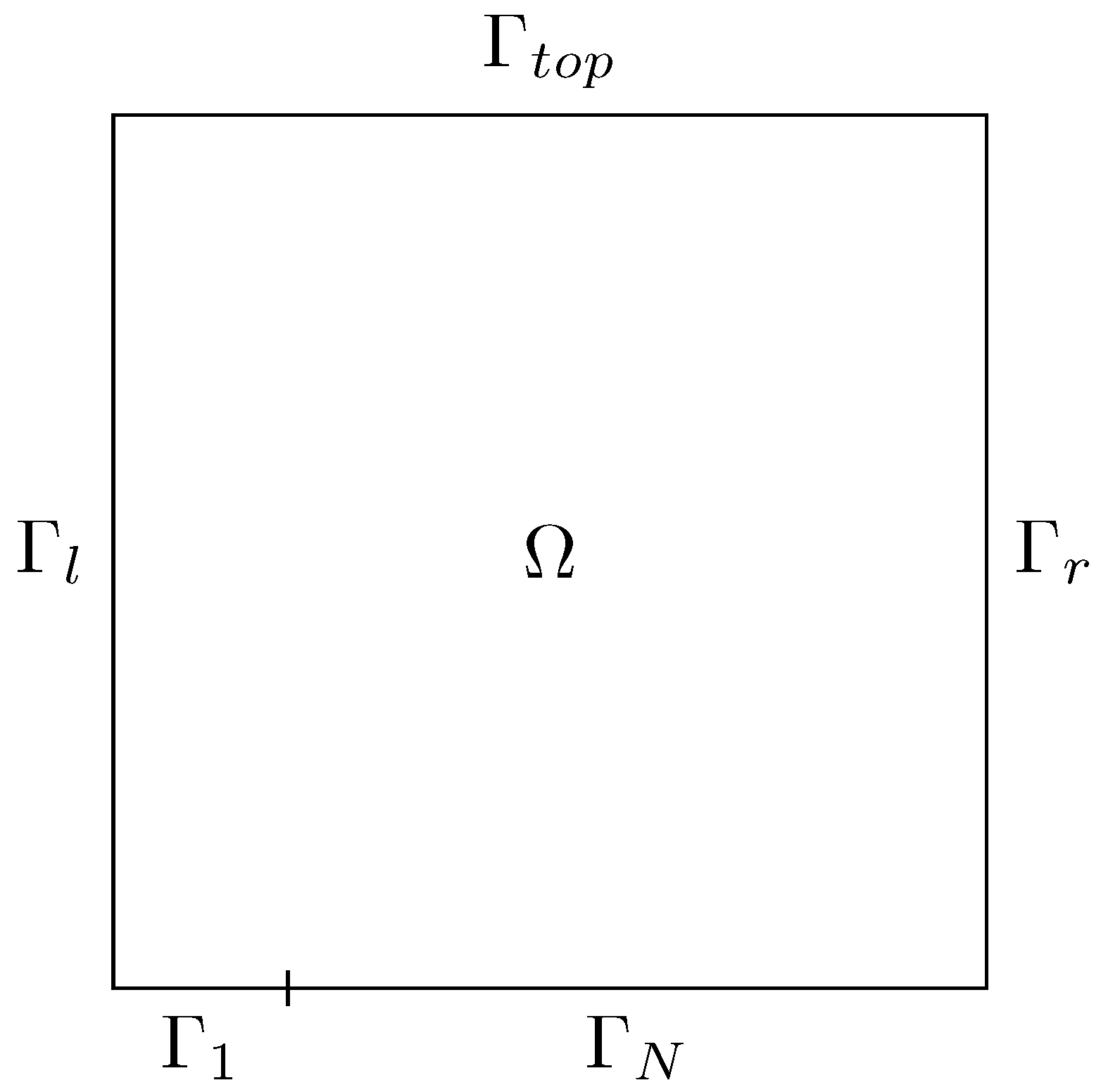
Figure 2.
Domain of the solid/fluid heat transfer problem.
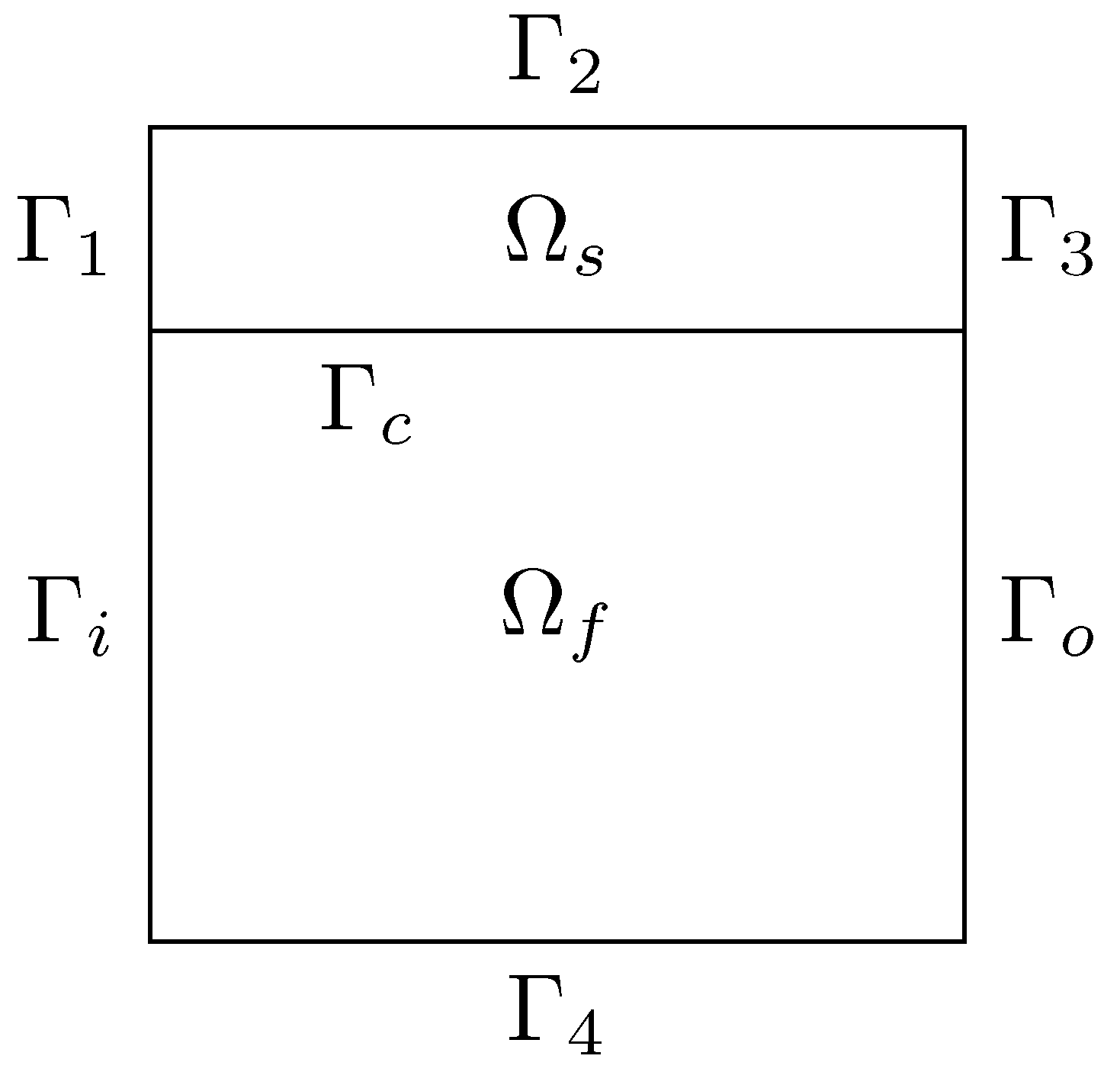
Figure 3.
Code coupling scheme for the optimal control of the Boussinesq system of equations.
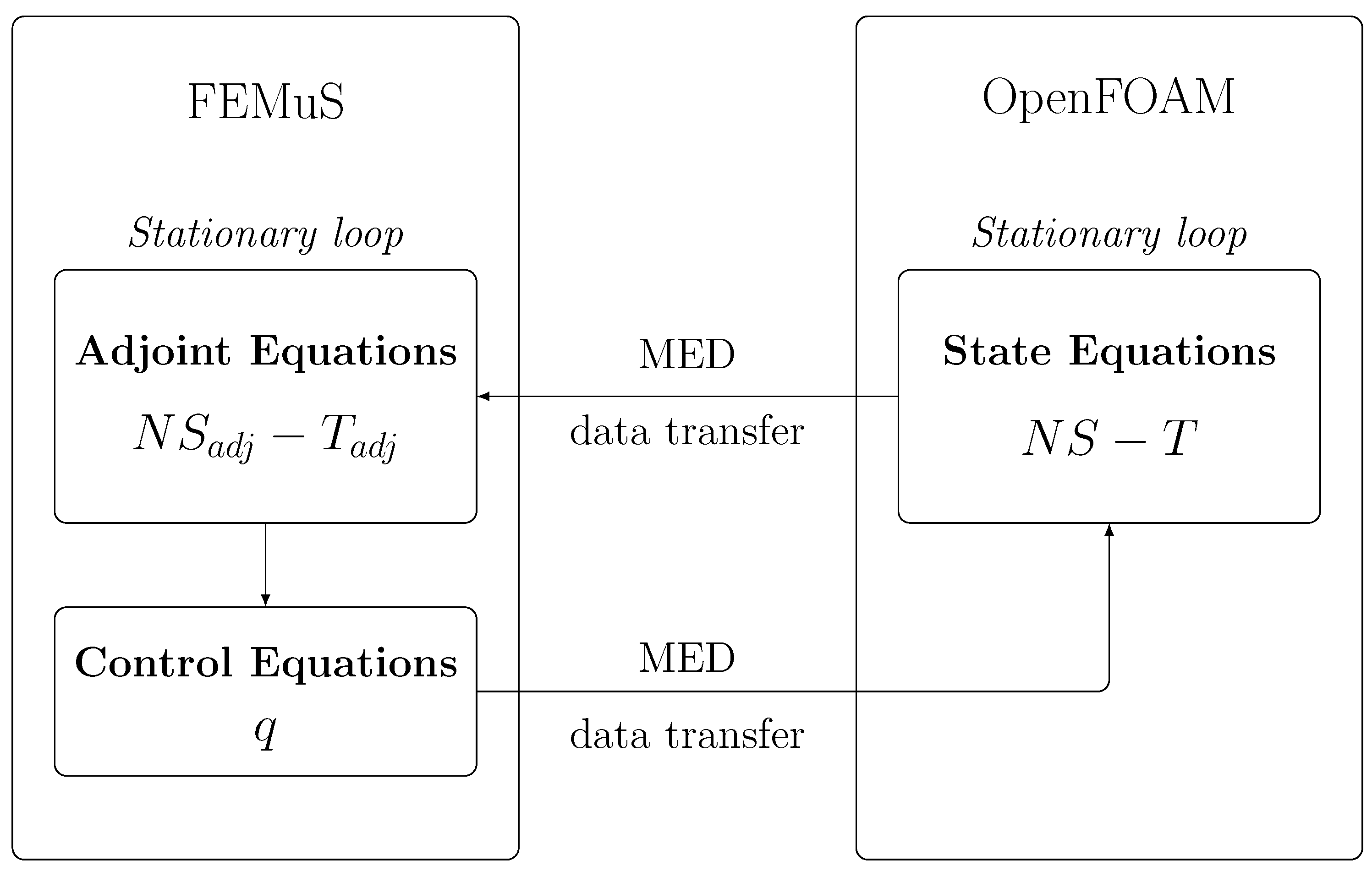
Figure 4.
Code coupling scheme for the optimal control of the CHT system.
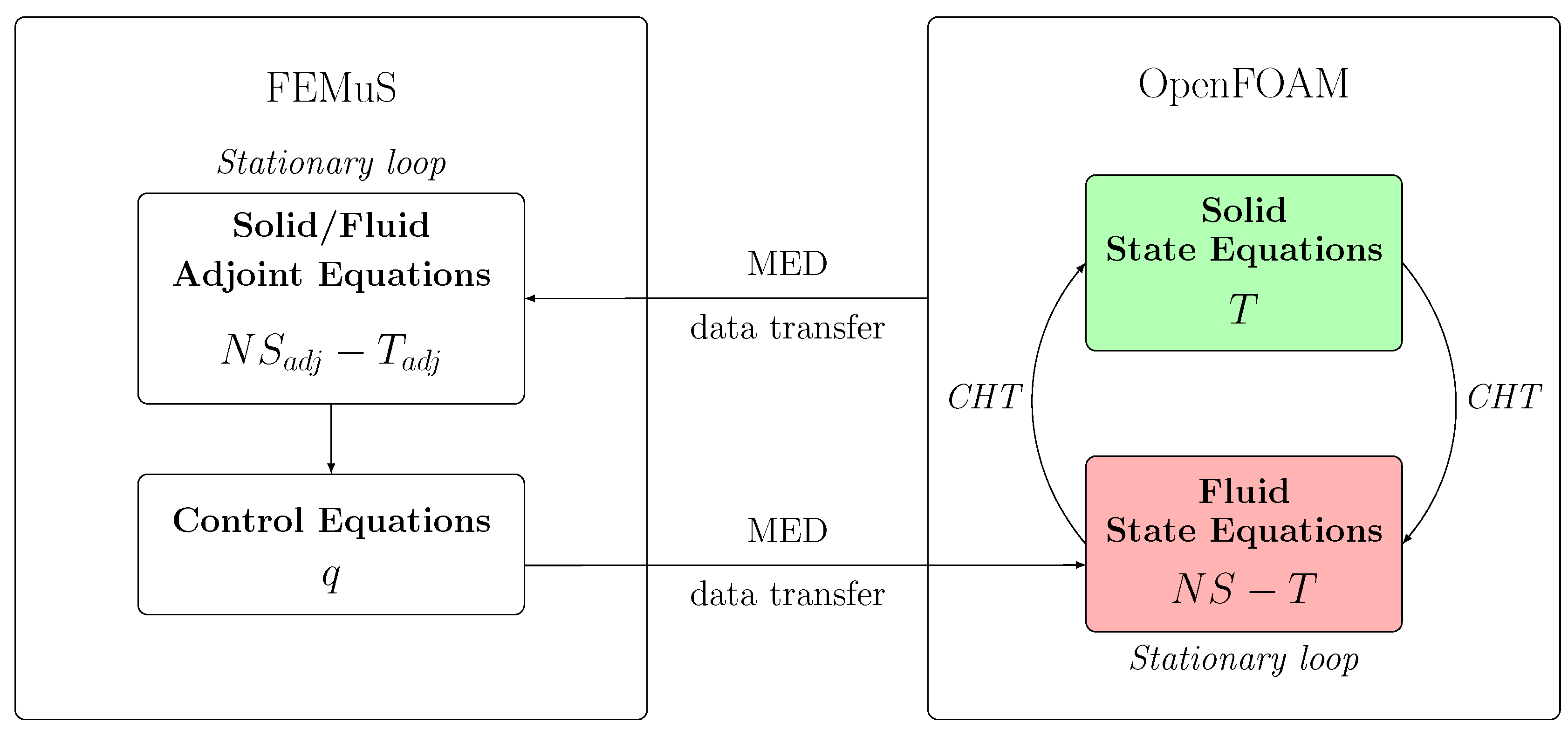
Figure 5.
Domain of the Rayleigh-Bénard minimization problem.
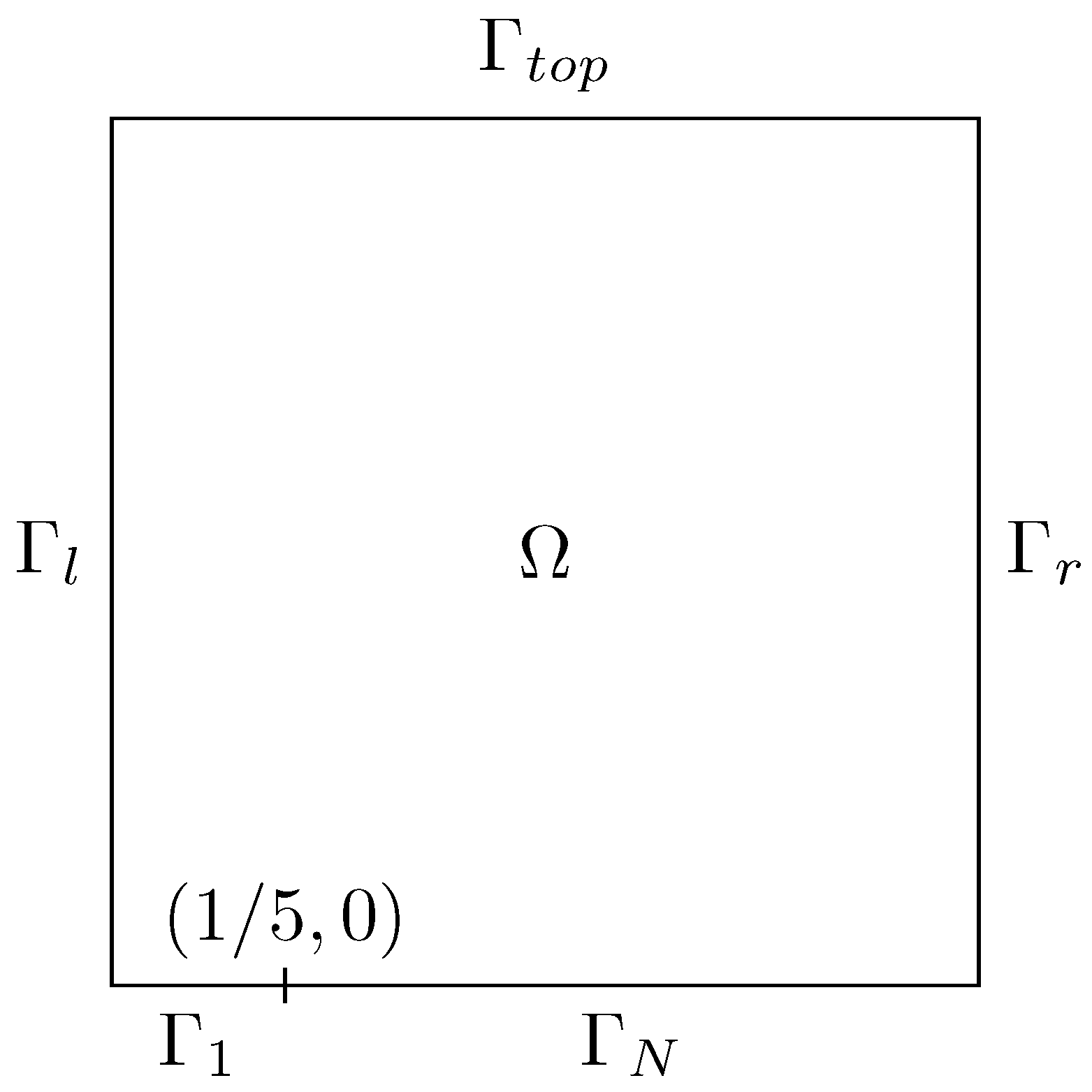
Figure 6.
The uncontrolled case: on the left, a contour plot of the temperature field; on the right, velocity glyph representation.
Figure 6.
The uncontrolled case: on the left, a contour plot of the temperature field; on the right, velocity glyph representation.
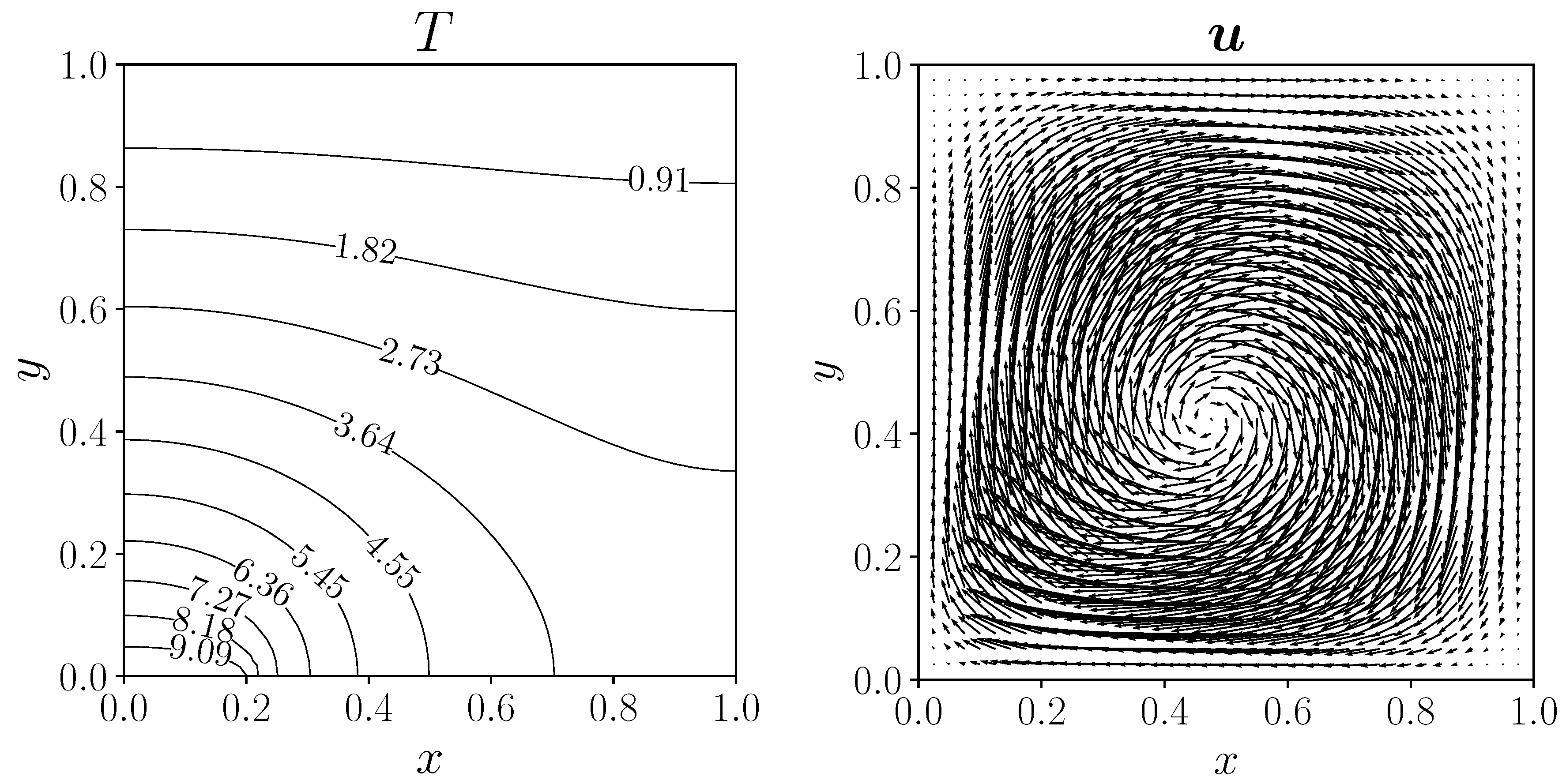
Figure 7.
Contour plot of the temperature field for the controlled cases, on the left and on the right. Solid line for the present results and dashed line for the reference case [3].
Figure 7.
Contour plot of the temperature field for the controlled cases, on the left and on the right. Solid line for the present results and dashed line for the reference case [3].
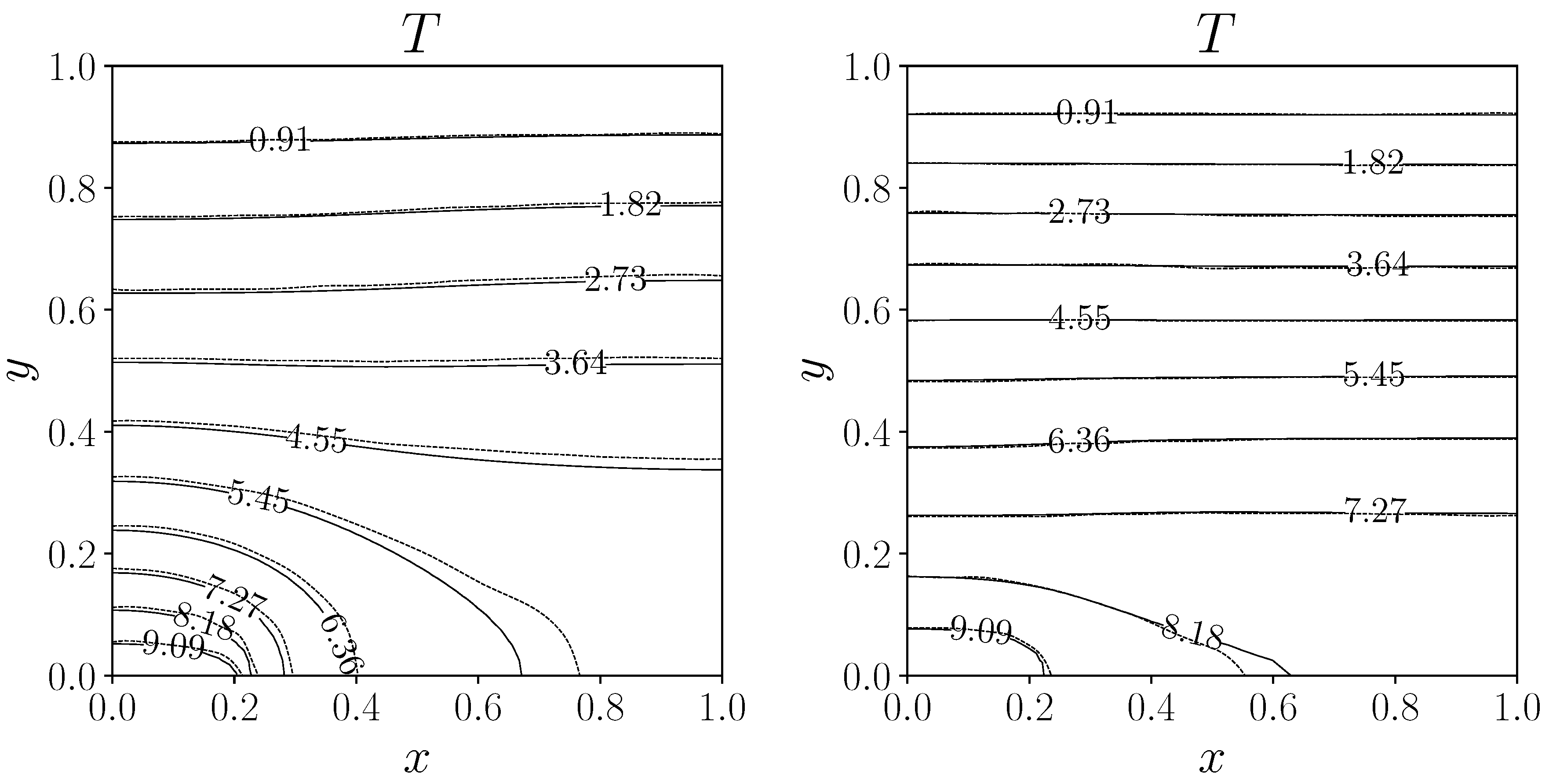
Figure 8.
Contour plot of control Q for the distributed case. On the left with , on the right with .
Figure 8.
Contour plot of control Q for the distributed case. On the left with , on the right with .
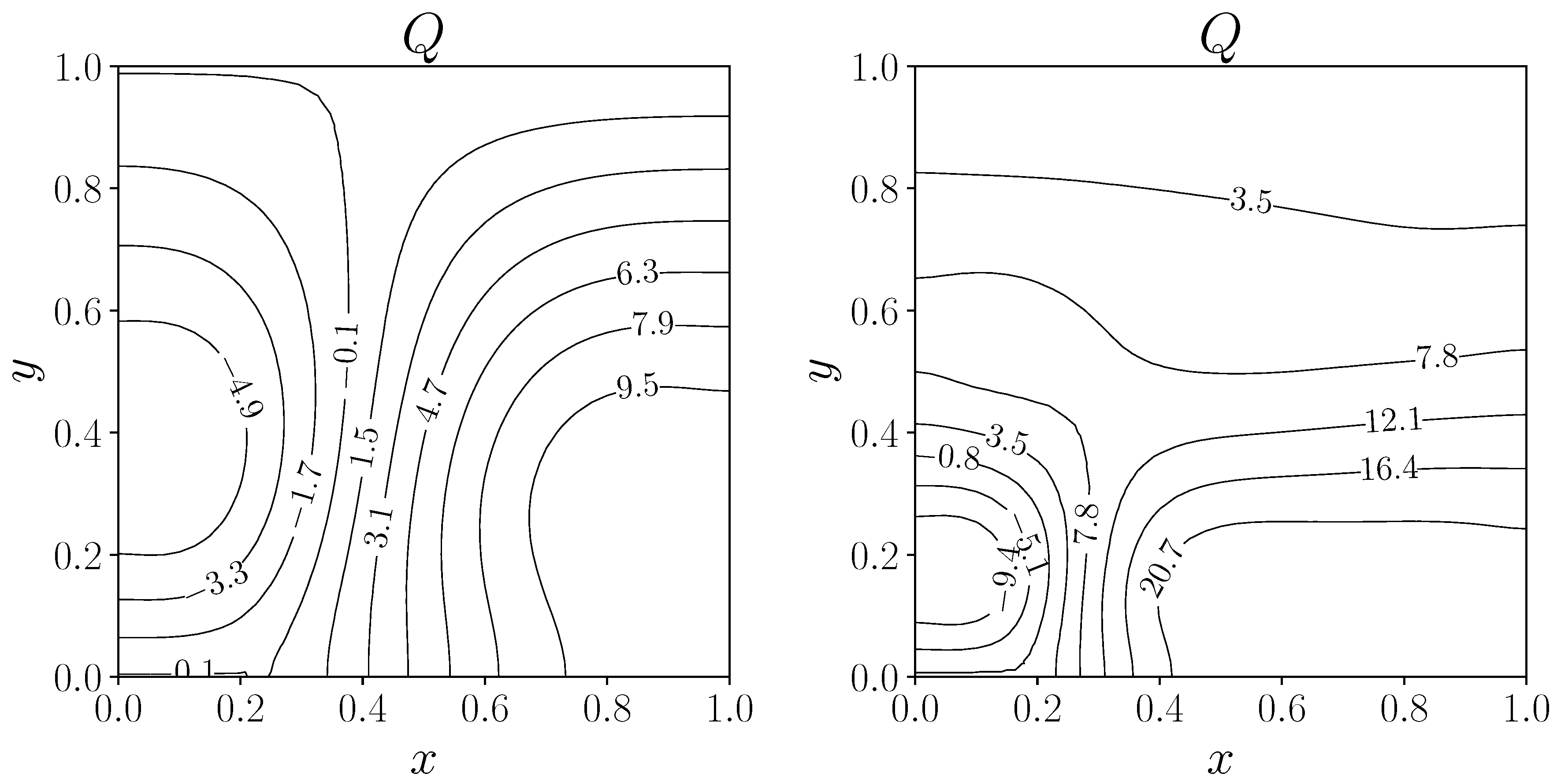
Figure 9.
Adjoint velocity field for the distributed case, on the left for , on the right for .
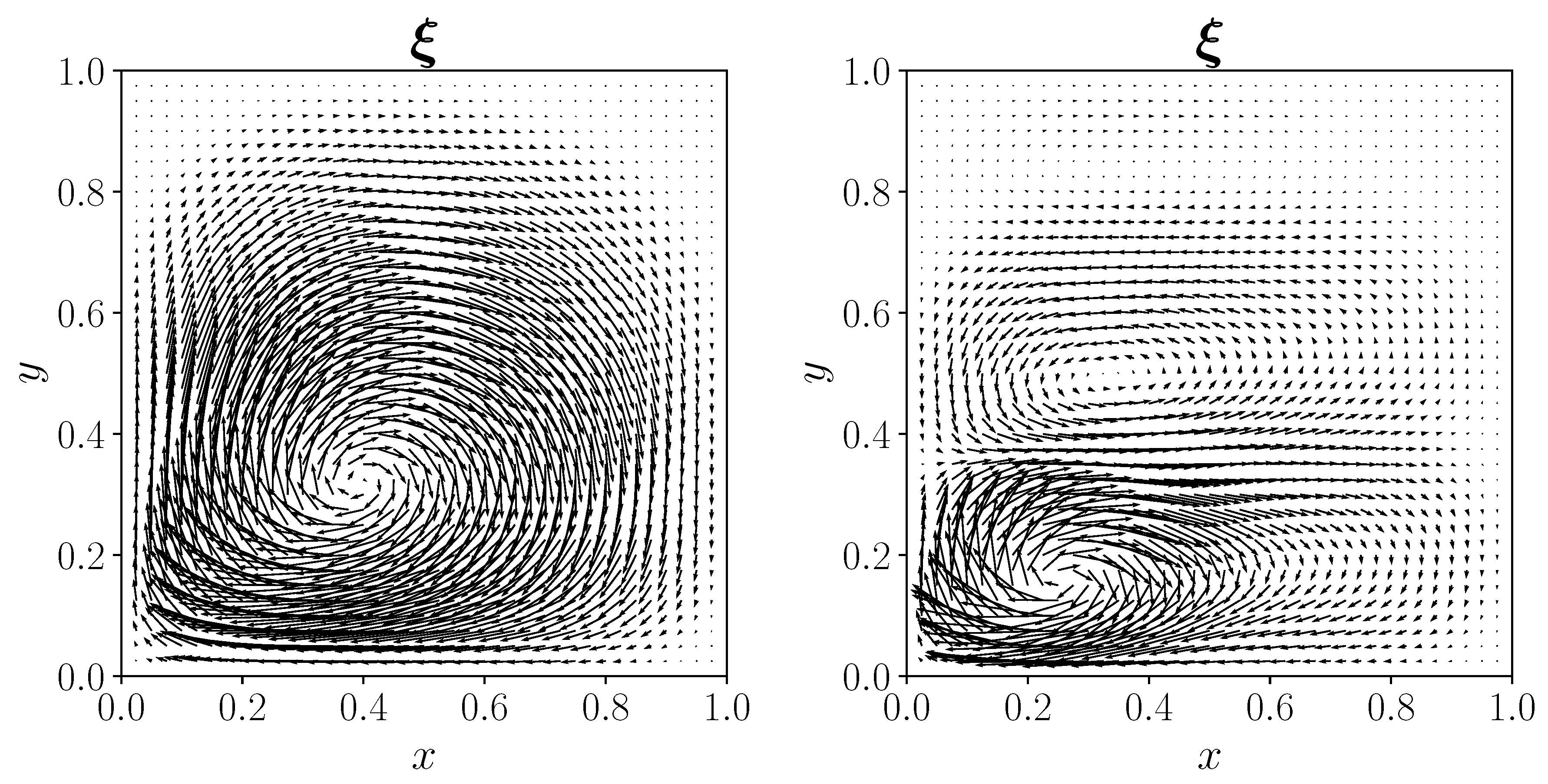
Figure 10.
Velocity field for the distributed case, on the left for , on the right for .
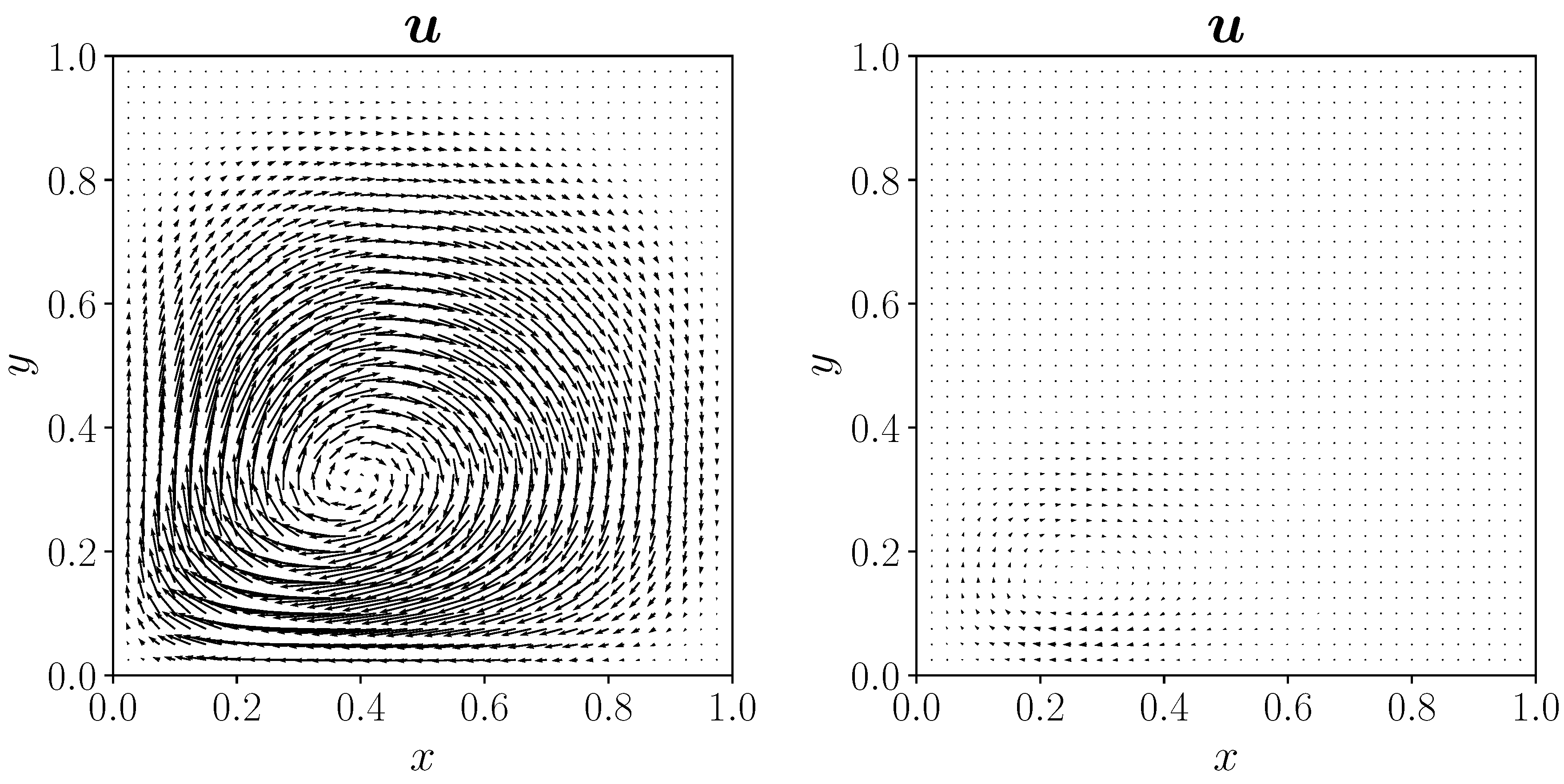
Figure 11.
Neumann boundary control for the two controlled cases on .

Figure 12.
Contour plot of the temperature field for the controlled cases, on the left and on the right. Solid line for the present results and dashed line for the reference case [3].
Figure 12.
Contour plot of the temperature field for the controlled cases, on the left and on the right. Solid line for the present results and dashed line for the reference case [3].

Figure 13.
Velocity field for the Neumann boundary control case, on the left for , on the right for .
Figure 13.
Velocity field for the Neumann boundary control case, on the left for , on the right for .
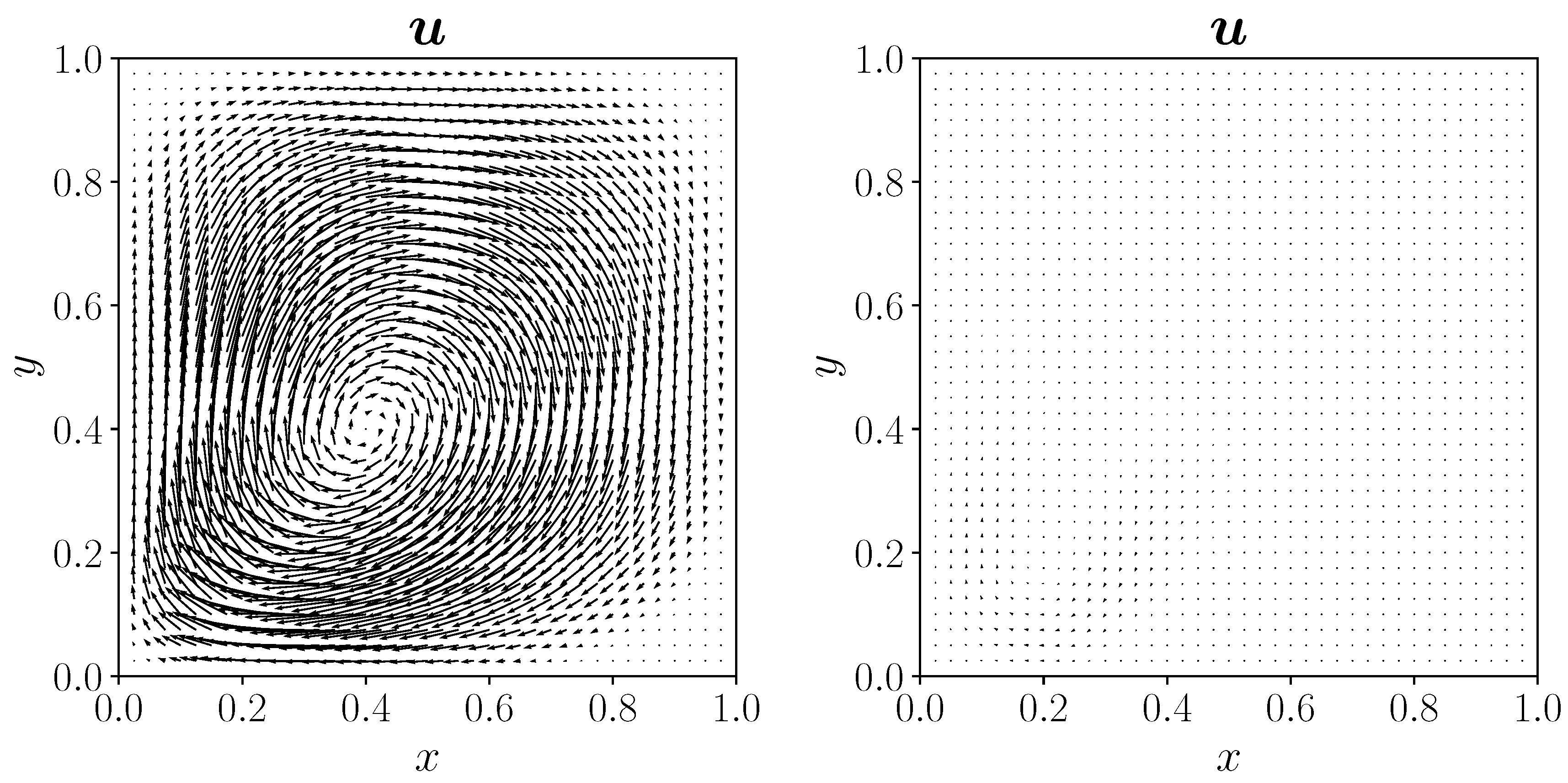
Figure 14.
Domain of the solid/fluid heat transfer problem.
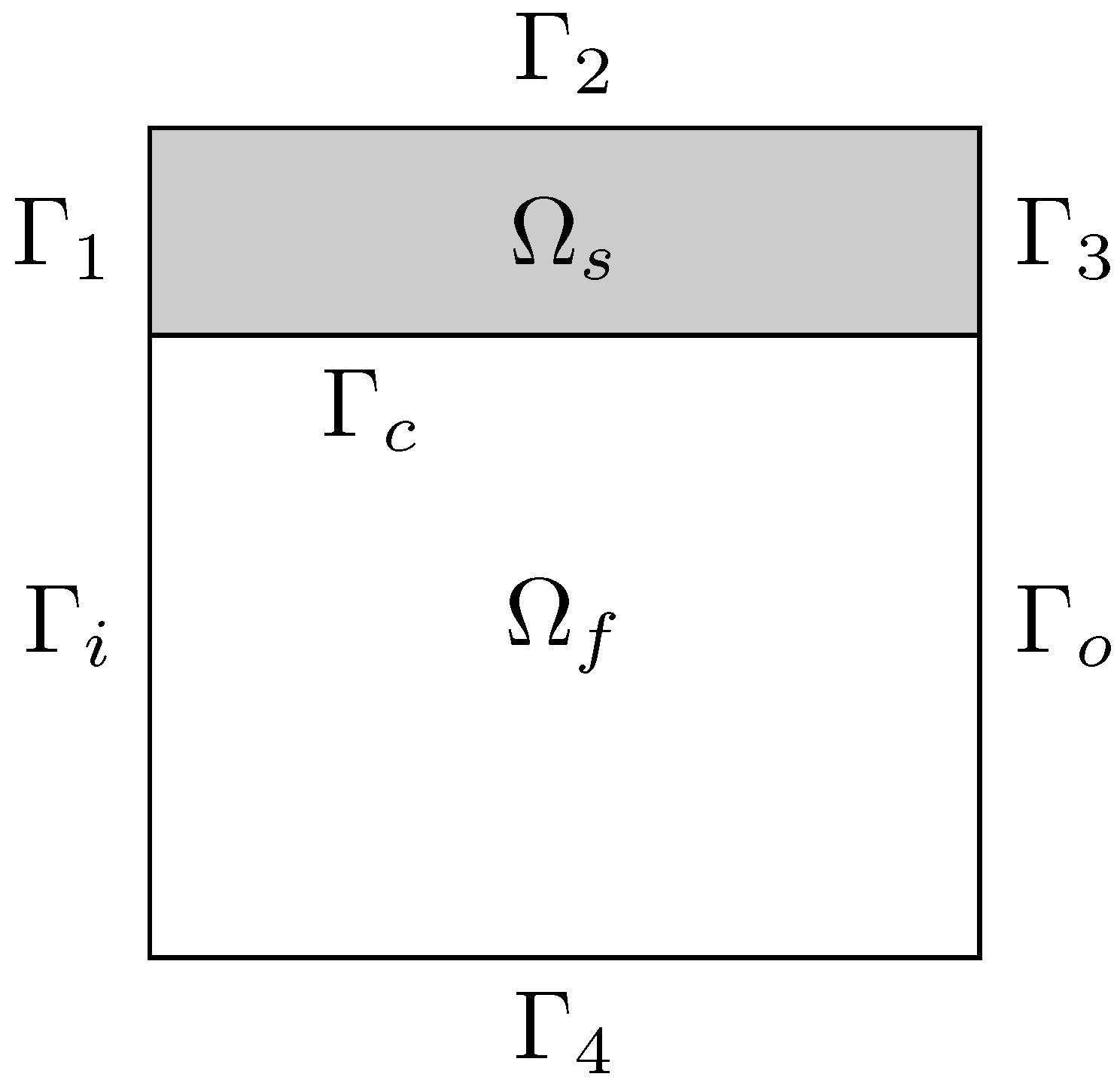
Figure 15.
On the left, target temperature isolines over ; on the right, target temperature profile on .
Figure 15.
On the left, target temperature isolines over ; on the right, target temperature profile on .

Figure 16.
Normal component of the control with respect to for the two controlled cases with different . Reference data [4] are reported with the circular markers.
Figure 16.
Normal component of the control with respect to for the two controlled cases with different . Reference data [4] are reported with the circular markers.
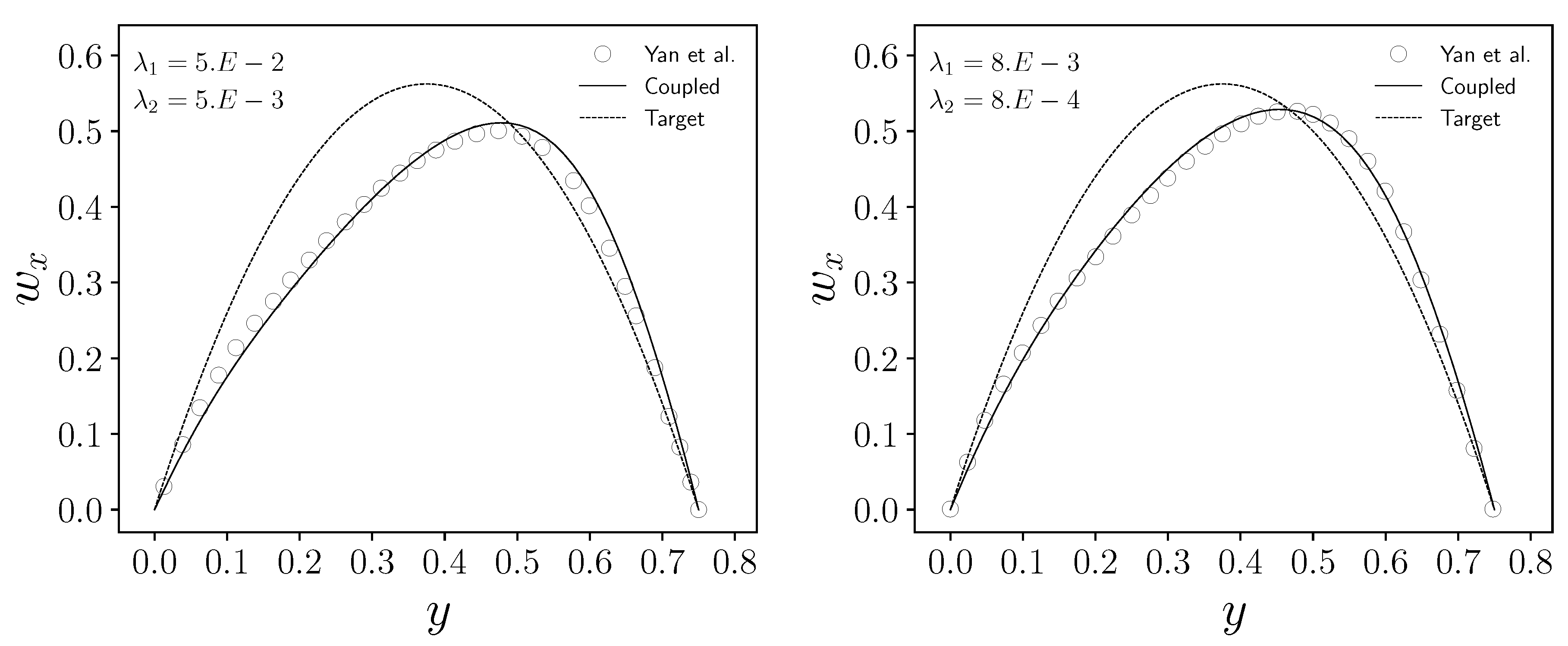
Figure 17.
Temperature profile on on the left, and corresponding relative temperature error on the right. Solid line for Case 1, dashed line for Case 2, dotted line for , and dash-dotted line for the initial temperature distribution associated to .
Figure 17.
Temperature profile on on the left, and corresponding relative temperature error on the right. Solid line for Case 1, dashed line for Case 2, dotted line for , and dash-dotted line for the initial temperature distribution associated to .
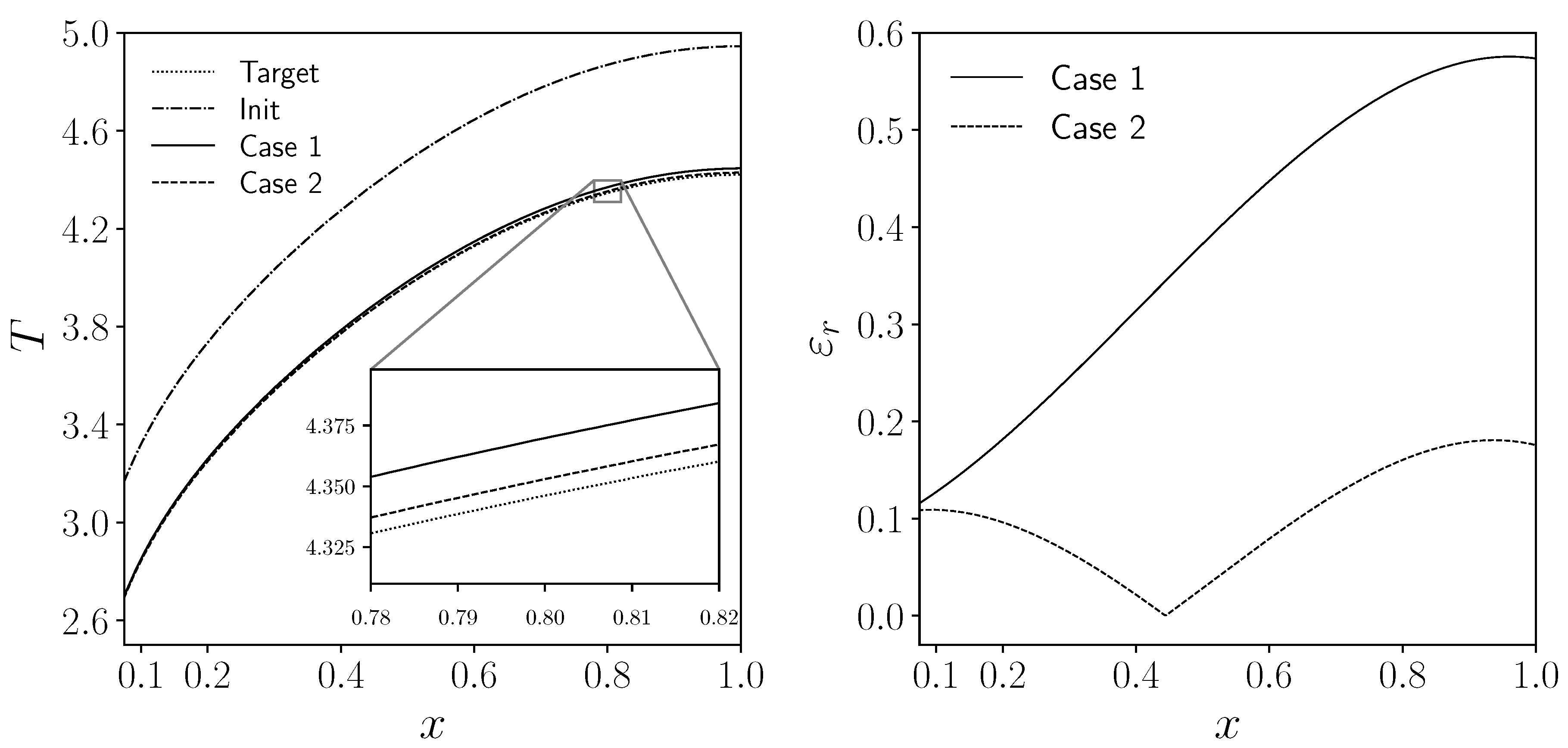
Figure 18.
Adjoint velocity (vector glyph) on the left and adjoint temperature (isolines) on the right. Case 1 on top, Case 2 on bottom.
Figure 18.
Adjoint velocity (vector glyph) on the left and adjoint temperature (isolines) on the right. Case 1 on top, Case 2 on bottom.
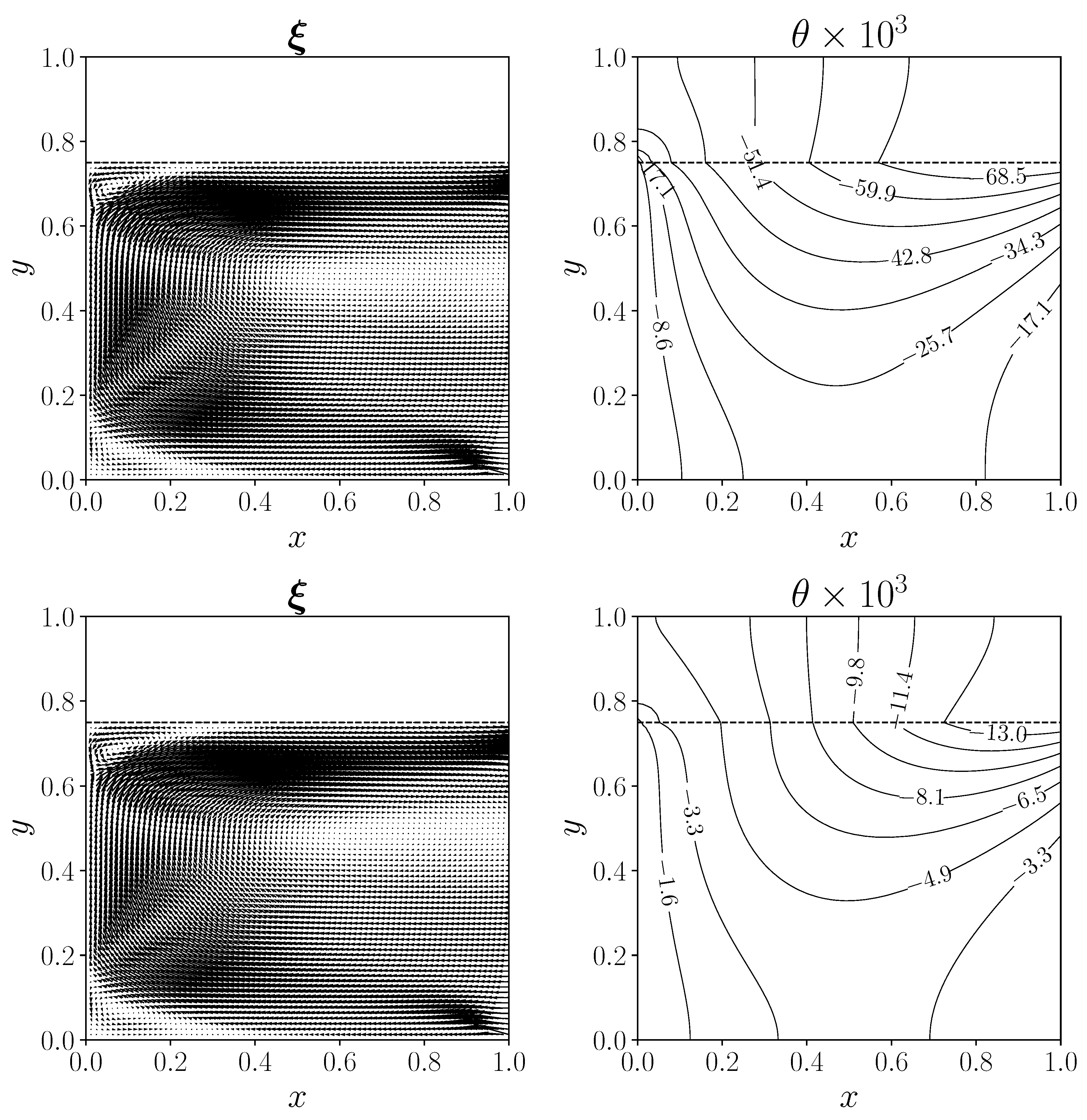

Table 1.
Boundary conditions for the Rayleigh-Bénard problem for each unknown on each portion of the boundary
Table 1.
Boundary conditions for the Rayleigh-Bénard problem for each unknown on each portion of the boundary
| T | |||||
Table 2.
Maximum velocity magnitude for the uncontrolled and distributed controlled cases.
| Uncontrolled | |||
|---|---|---|---|
Table 3.
Cost functionals for the vorticity minimization with a distributed control. In the last column, the relative error of the total functional is reported.
Table 3.
Cost functionals for the vorticity minimization with a distributed control. In the last column, the relative error of the total functional is reported.
| C | [3] | C | [3] | C | [3] | ||
|---|---|---|---|---|---|---|---|
| Uncontrolled | - | - | |||||
Table 4.
Maximum velocity magnitude for the uncontrolled and Neumann boundary controlled cases.
| Uncontrolled | |||
|---|---|---|---|
Table 5.
Cost functionals for the vorticity minimization with a Neumann boundary control. In the last column, the relative error of the total functional is reported.
Table 5.
Cost functionals for the vorticity minimization with a Neumann boundary control. In the last column, the relative error of the total functional is reported.
| C | [3] | C | [3] | C | [3] | ||
|---|---|---|---|---|---|---|---|
| Uncontrolled | - | - | |||||
Table 6.
Boundary conditions for the solid/fluid CHT problem.
| - | - | - | |||||
| T | CHT | ||||||
| - | - | - | |||||
| CHT |
Table 7.
Cost functionals for the temperature minimization with a Dirichlet boundary control on the velocity inlet value.
Table 7.
Cost functionals for the temperature minimization with a Dirichlet boundary control on the velocity inlet value.
| Uncontrolled | - | ||||
Table 8.
Convergence order p for the Rayleigh-Bénard control case.
| p | ||||
Table 9.
Convergence order p for the Solid-Fluid control case.
| Case 1 | Case 2 | |
|---|---|---|
| p |
Disclaimer/Publisher’s Note: The statements, opinions and data contained in all publications are solely those of the individual author(s) and contributor(s) and not of MDPI and/or the editor(s). MDPI and/or the editor(s) disclaim responsibility for any injury to people or property resulting from any ideas, methods, instructions or products referred to in the content. |
© 2025 by the authors. Licensee MDPI, Basel, Switzerland. This article is an open access article distributed under the terms and conditions of the Creative Commons Attribution (CC BY) license (http://creativecommons.org/licenses/by/4.0/).
Copyright: This open access article is published under a Creative Commons CC BY 4.0 license, which permit the free download, distribution, and reuse, provided that the author and preprint are cited in any reuse.