

Submitted:
07 April 2025
Posted:
07 April 2025
You are already at the latest version
Abstract
In this study, twelve modified differential evolution algorithms with memory properties and adaptive parameters were proposed to solve the optimization problem. In the experimental process, these modified differential evolution algorithms were applied to 23 continuous test functions. Experiments show that MBDE2 and IHDE-BPSO3 are superior to the original differential evolution algorithm and its extended variants, and the best solutions can be found in most of the problems. It is inducted that the proposed improved differential evolution algorithm can adapt to most problems and obtain better results, and adding the concept of memory property is a great improvement to the capability of the proposed improved differential evolution algorithm.
Keywords:
differential evolution
; particle swarm optimization
; self-adaptive parameters
; optimization
1. Introduction
Differential evolution algorithm [1] is a fairly mainstream heuristic algorithm, which has been studied and improved by most studies [2,3,4,5,6,7,8,9,10,11]. Because the process is fast and simple, it is very suitable for solving optimization problems with less time consuming. However, the differential evolution algorithm does not guarantee that the global optimal solution can be found, so under this problem, the differential evolution algorithm has developed a variety of mutation algorithms. The mutation algorithm refers to the part that generates a random solution, such as DE/rand/1 or DE/rand/2, or changes the formula of the algorithm to form a new algorithm. To compare novel algorithms, the differential evolution algorithm and its deformation still maintain a good position in most problems, indicating that the diversity of variation in the selection of mutation algorithms is quite important. The weight-changing differential evolution algorithm used in this study has maintained good results in previous studies. The parameter settings are based on the user's past experience, and the concept of memory is rarely used in the original differential evolution algorithm. Although the original differential evolution algorithm can have good results in the average performance, it cannot get good results with the same parameter settings for various problems. Therefore, in this study, a different differential evolution algorithm is proposed to improve the concepts of adaptive and memory, and it is named the Improved Hybrid Differential Evolution Algorithm (IHDE). In this paper, the concept of particle swarm optimization algorithm is tried to influence the structure of the solution generated by the formula, so that it can achieve good results on most problems.
2. Related Works
Storn and Price [1] published a differential evolution algorithm in 1997, which is classified as an intelligent optimization algorithm. At the beginning, the differential evolution algorithm will first set the basic parameters, including group size, scaling factor, and crossover probability and so on, and generate an initial set of solutions x based on the upper and lower bounds of the given solution and according to rand (0, 1). Then, the initial solution x is mutated to generate a mutation solution, and then the structure of the solution is changed by means of crossover probability to produce a crossover solution x′. In the selected section, if a cross solution x′ is better than the current solution x, the original initial solution is replaced by a cross solution, otherwise, nothing replaced. The algorithm repeats the mutation, crossover, and selection until the end of the iteration. Figure 1 shows the conceptual diagram of the differential evolution algorithm. This example takes dimension size 2 as an example, showing the outline of the algorithm and the process of generating the mutation solution, which is the result of the weighted difference of the initial value of two arbitrary selections and the addition of the third value to obtain the mutation solution. In the figure, V is the mutation solution; X is the initial solution; F is the scaling factor; G is the iteration; and each of is a random group with no repetitions.
The differential evolution algorithm is also a stochastic model that simulates biological evolution, through multiple iterations and preserves those individuals who are better adapted to the environment. The advantage of differential evolution algorithms is with shorter steps compared to other algorithms. There are only four steps: initialization, mutation, crossover, and selection. Therefore, the convergence time of the algorithm is relatively less than other algorithm, but it still retains strong global convergence ability and robustness.
Particle swarm optimization (PSO) algorithm concept was proposed by two scholars, Kennedy and Eberhart [12]. At the beginning, set parameters including population size, inertia weight, acceleration constant, maximum velocity, and etc. A random swarm of particles is then generated, and their position is adjusted based on the individual experience of each particle's flight and the best experience in the past. The particles produced at the beginning can be treated as a set of solutions x, and their velocity equation v, the individual optimal position (pbest), and the global optimal position (gbest) affect the individual position of the next iteration. The algorithm then iteratively finds the best position (i.e., the best solution), and the algorithm continues until the end of the iteration or reaches the given max_steps. Figure 2 is a conceptual diagram of the particle swarm optimization algorithm, where k is the iteration, pbest is the individual optimal position, gbest is the global optimal position, x is the initial solution (or contemporary solution), v is the velocity, and new x and v will be generated according to the following formula.
The main framework of the particle swarm optimization algorithm is to generate the initial solution and initial velocity, and then update the velocity and position according to the velocity and position formula until the end of the iteration. The formula is as follows:
Velocity update formula:
where v is the velocity, t is the iteration, X is the contemporary solution, pbest is the individual optimal position, gbest is the global optimal position, and c1 and c2 are the acceleration constants, ω is the inertia weight, r1, and r2 are random values between 0 and 1.
Position update formula:
In the position update formula, a new particle position can be obtained, which is the contemporary solution for the next iteration. The speed update formula and the position update formula are repeated until the end of the iteration or until the user-set stop condition is reached.
There are many variations of differential evolution algorithms, among which Qin and Suganthan [14] proposed a differential evolution algorithm for two mutation algorithms at the same time(Self-adaptive Differential Evolution, SaDE); Huang et al. [15] proposed a differential evolution algorithm of the cooperative evolution(Co-evolutionary Differential Evolution, CDE). The whole part is divided into two groups with interaction, and the algorithm also affects each other when it is carried out.
Parouha and Das [16] proposed a modified differential evolution algorithm called MBDE (Memory based Hybrid Differential Evolution). In this paper, the formula of the differential evolution algorithm is added to the memory method, and the individual optimal position and the global optimal position are introduced to change the concept that the past solution of the differential evolution algorithm does not affect the future generation solution. And then, the mutation and crossover steps are changed to Swarm Mutation and Swarm Crossover, and finally the greedy selection method is improved to Elitism, which greatly improves the overall algorithm performance. The improved formula is shown as follows:
Improved Swarm Mutation:
In this part, the original mutation algorithm DE/rand/2 takes into account the concept of memory, where V is the mutation solution, t is the iteration number, X is the contemporary solution, pbest is the individual best position, gbest is the global best position, is the contemporary worst solution, and f (∙) is the objective function.
Improved Swarm Crossover:
The crossover algorithm also takes into account the concept of memory, where V is the mutation solution, t is the iteration number, X is the contemporary solution, pbest is the individual best position, gbest is the global best position, rand(0, 1) and randij. are random real numbers between 0 and 1, and pcr. is the user-defined crossover probability.
Elitism:
This part is to change the original greedy choice method to the elite choice method. This method is proposed to discard the overall algorithm diversity, because the diversity has been processed in the previous mutation step and the cross step, so there is no need to deal with it in this part. Whereas, elitism obeys the following three rules:
- (1)
- In the final elite selection section, the initial population (or contemporary target vector) and the resulting species from the final crossover are combined.
- (2)
- The merged populations will be sorted in ascending order according to the value of the target function.
- (3)
- The better NP (population number) individuals are retained to move on to the next iteration, and the remaining individuals are allowed to be removed.
Chen et al.[17] proposed HPSO (Hybrid Particle Swarm Optimizer), in which the parameters required for the original PSO formula were brought into the concept of adaptation, and the formula was improved for generating target value and velocity of next step. The acceleration constant algorithm is based on the TVAC(Time Varying Acceleration Coefficient) commonly used in the past literature and the inertia weight is modified. The modified formula is as follows:
Velocity update formula:
where, χ replaces the inertia weight and further affects the individual optimal position and the proportion of the global optimal position on the velocity, v is the velocity, t is the iteration number, X is the contemporary solution, pbest is the individual optimal position, and gbest is the global optimal position.
Position update formula:
where u is the average value of the initial population substituting the objective function, and f(∙) is the objective function. This improvement greatly reduces the problem of user parameter setting. For parameter adaptation, the parameter values can be changed according to iterations, so that the algorithm can produce different results in different iteration periods. The proportion of the individual optimal position and the global optimal position can also be changed according to the needs of the algorithm and the progress of iteration. The acceleration constant is set by the adaptive algorithm commonly used in previous literature, and the overall velocity update formula is affected by another inertia weight.
Hizarci et al. [13] proposed Binary Particle Swarm Optimization (BPSO), which is different from the previous method in that it sets an adaptive algorithm with a speedup constant. The acceleration constant algorithm commonly used in the past is abandoned, and the inertia weight is adaptive, so that it can reduce the impact of the speed of the previous iteration according to the iteration. For the other formulas, it is a formula that uses the original particle swarm optimization algorithm entirely. The acceleration constant adaptation and inertia weight adaptation formulas are as follows:
Acceleration constant formula:
where = 0.5, = 2.5, iter is the iteration at that time, is the maximum number of iterations.
Inertia weight formula:
where = 0.9 , and = 0.4.
Based on the review of the above papers, it can be found that the differential evolution algorithm with memory properties has good performance and can effectively deal with the problem of group diversity. The acceleration constant, which has a lot of influence on the velocity formula of the particle swarm optimization algorithm, is nothing more than a factor that has a great influence. In this study, we will consider applying the formula of particle swarm optimization to the differential evolution algorithm. and continue the other steps of the differential evolution algorithm to intersect to disrupt the structure of the solution. The target algorithm can have the ability to adapt to most problems and have good results.
3. The Proposed Method
In this paper, twelve modified differential evolution algorithms were proposed. The proposed algorithm can be divided into four parts, namely:
- (1)
- Simply increase the selection group.
- (2)
- Added additional cross-solutions based on contemporary solutions.
- (3)
- The crossover step uses the mutated solution as the base to generate a new crossover solution.
- (4)
- Differential evolution algorithms are improved based on the improved particle swarm algorithm.
The basic concepts and corresponding algorithms of these four classifications are described in Table 1.
Simply increase the selecting individuals (MBDE_2): The concept is that the original MBDE algorithm has a good effect, but it is hoped that the algorithm can find more and better solutions quickly in the early stage by taking advantage of the large search range of mutation solutions. Therefore, the overall structure and formula of the original MBDE are retained. Changed the selection section so that it also takes mutants into account when selecting them.
MBDE2:
Mutation:Make use of formula (3).
Crossover:
Selection:Contemporary solutions, variant solutions and cross-solution , to retain good NP (population) individuals to the next iteration.
The concept of IHDE, IHDE_2 and IHDE_2cross based on contemporary solutions to generate additional crossover solutions is mainly to propose a new crossover formula. This new crossover formula will be related on contemporary solution-based vectors. In this study, the mutation solution can already be used as a group of independent individuals to compete with other individuals. So the new cross-solution part doesn't have any effect on the mutated solution. Finally, the three algorithms consider different steps to choose separately.
IHDE:
Mutation:Make use of formula (3).
Crossover:Make use of formula (10) to obtain crossover solution .
Selection:Select the mutation solution and crossover solution , and retain the better NP (population number) individuals to the next iteration.
IHDE - 2:
Mutation:Make use of formula (3).
Crossover:
Selection:Select the contemporary solution , mutation solution and crossover solution , and retain the better NP (population number) individuals to the next iteration.
IHDE - 2cross:
Mutation:Make use of formula (3).
Crossover 1:Make use of formula (9) to obtain crossover solution.
Crossover 2:Make use of formula (10) to obtain crossover solution.
Selection:Select the contemporary solution , mutation solution and crossover solution and , and retain the better NP (population number) individuals to the next iteration.
The IHDE_mgi and IHDE_mgm are based on the crossover step that is to generate in a new crossover solution based on the mutated solution. The main concept of these two algorithms is that although the mutated solution is sufficient to be used as a solution to compete with other individuals to become the next generation, its wide search range can be better if it is used to influence again with past memories at the crossover step. Therefore, these two algorithms are proposed, and these two algorithms are slightly different in the intersection part.
IHDE - mgi:
Mutation:Make use of formula (3).
Crossover:
Selection:Select the contemporary solution , mutation solution and crossover solution, and retain the better NP (population number) individuals to the next iteration.
IHDE - mgm:
Mutation:Make use of formula (3).
Crossover:
Selection:Select the contemporary solution , mutation solution and crossover solution, and retain the better NP (population number) individuals to the next iteration.
Improved IHDE_BPSO3, IHDE_BPSO4 and IHDE_BPSO5 based on different algorithms of Binary Particle Swarm Optimization (BPSO). BPSO is used because it proposes a new adaptive acceleration constant algorithm. In the study of Hizarci et al. [13], this adaptive algorithm has obtained a good ranking compared with the adaptive algorithm commonly used in the previous literature of particle swarm optimization algorithms, and has shown potential effects. Therefore, the speed and position of BPSO can be used to update the formula and its adaptive algorithm to generate different mutation solutions and crossover solutions. And in two of these algorithms, new cross-solutions are generated, which disrupt the structure of the solution in a probabilistic way.
IHDE - BPSO3:
Mutation:Make use of formula (1) and (7). The parameters of the mutation part are set also using equation (7).
Crossover:Make use of formula (9).
Selection:Select the contemporary solution , mutation solution and crossover solution, and retain the better NP (population number) individuals to the next iteration.
IHDE - BPSO4:
Mutation 1:Make use of formula (1) to obtain mutation solution
Mutation 2:Make use of formula (2) to obtain mutation solution . The parameters of the mutation part are set also using equations (7) and (8).
Crossover 1:Make use of formula (9) to obtain crossover solution
Crossover 2:
is set to 0.5, because the variant solution 2 generated based on BPSO will be better, so it is hoped that the structure of the solution will be affected with a greater probability. However, is set to 0.75, so that the mutated solution 1 and the contemporary solution can affect the structure of the solution with a small probability.
Selection:Select the contemporary solution , mutation solution and crossover solution and , and retain the better NP (population number) individuals to the next iteration.
IHDE - BPSO5:
Mutation 1:Make use of formula (1) to obtain mutation solution
Mutation 2:Make use of formula (2) to obtain mutation solution The parameters of the mutation part are set also using equations (7) and (8).
Crossover 1:Make use of formula (9) to obtain crossover solution
Crossover 2:Make use of formula (13) to obtain crossover solution
Selection:Select the contemporary solution , mutation solution and and crossover solution and , and retain the better NP (population number) individuals to the next iteration.
Improved IHDE_HPSO3, IHDE_HPSO4 and IHDE_HPSO5 based on different algorithms of improved particle swarm optimization. The idea of using HPSO is due to the addition of novel adaptive methods to the velocity update formula and position update formula, as well as the change from weights that only affect the previous generation of generation velocity solutions to affect the entire velocity formula. Then, there are many improvements to the adaptive parameters, so the proposed method integrates its concepts into the algorithm architecture to generate different solutions.
IHDE - HPSO3:
Mutation:Make use of formula (5).
Crossover:Make use of formula (9).
Selection:Select the contemporary solution , mutation solution and crossover solution, and retain the better NP (population number) individuals to the next iteration.
IHDE - HPSO4:
Mutation 1:Make use of formula (5) to obtain mutation solution
Mutation 2:Make use of formula (6) to obtain mutation solution
Crossover 1:Make use of formula (9) to obtain crossover solution.
Crossover 2:Make use of formula (13) to obtain crossover solution
Selection:Select the contemporary solution , mutation solution and crossover solution and , and retain the better NP (population number) individuals to the next iteration.
IHDE - HPSO5:
Mutation 1:Make use of formula (5) to obtain mutation solution
Mutation 2:Make use of formula (6) to obtain mutation solution
Crossover 1:Make use of formula (9) to obtain crossover solution.
Crossover 2:Make use of formula (13) to obtain crossover solution
Selection:Select the contemporary solution , mutation solution and and crossover solution and , and retain the better NP (population number) individuals to the next iteration.
4. Experimental Results
In subsection 4.1, it will introduce the optimization problems to be tested in this study, and run in Python 3.7, with an Intel(R) Core(TM) i7-9700 CPU @ 3.00GHz, an Intel UHD Graphics 630 GPU, and 16.0 GB of RAM. Then, in subsections 4.2 and 4.3, the results of the differential evolution algorithm are compared with most well-known algorithms. From the results, it can be seen that the original differential evolution algorithm has good performance among many algorithms. Finally, in subsection 4.4, the comparison between the improved differential evolution algorithm and the original differential evolution algorithm and its variants is presented.
4.1. Benchmark Functions
In order to test the performance of the proposed improved differential evolution algorithm, 23 test functions used in the study of Abualigah et al.[18] were used to test the performance of the original differential evolution algorithm to be improved, as shown in Table 2, Table 3 and Table 4. These test functions contain unimodal test functions, multimodal test functions, and fixed-dimension multimodal test functions.
The unimodal test functions F1~F7 will be tested at dimension 30 and set 30 with the initial group number, set the number of iterations to 500, and test the above test settings with 30 average results, and the range of each function is shown in Table 2.
The multimodal test functions F8 to F13 will be tested in 30 dimensions, the initial population number of 30, the number of iterations 500, and the average of 30 tests will be used as the basic settings, and the range are shown in Table 3.
The fixed-dimension multimodal functions from F14 to F23 are set to the initial population of 30, the number of iterations is 500, and the average of 30 tests is set as the basic settings, and its dimensions and ranges are shown in Table 4.
All kinds of test functions in unimodal, multimodal and fixed-dimension multimodal test functions can detect the convergence speed of the algorithm, the ability of the algorithm to jump out of the part and the convergence ability of the algorithm as a whole, and most of these test functions belong to the test functions with high search difficulty, so the prototype of most well-known algorithms may not be able to find the best value, even the emerging variants of the algorithm are the same. The algorithm in this study will test the formulas of the improved differential evolution algorithm and its adaptive parameter settings, and the parameters will no longer be set in a random or fixed way, and can obtain good results in these test functions, so that the performance of the algorithm can be effectively improved.
In the unimodal, multimodal and fixed-dimension multimodal test functions, the convergence speed of the algorithm, the ability of the algorithm to jump out of the locality, and the convergence ability of the algorithm as a whole can be detected. Most of these test functions are difficult to search, so prototypes of most well-known algorithms do not necessarily find optimal values, even for emerging variants of algorithms. In recent years, some scholars have been proposing new algorithms, various algorithm variants, or changing their parameter settings to cope with these complex test functions. The proposed algorithm will test the formulas of the improved differential evolution algorithm and its adaptive parameter settings. The experimental results show that good results can be obtained in these test functions, and the performance of the algorithm can be effectively improved.
4.2. Algorithm and Parameter Settings Compared with the Original Differential Evolution Algorithm
This subsection introduces the basic parameter settings of the original differential evolution algorithm and 11 well-known algorithms to be improved in this study. With the exception of the original differential evolution algorithm, all parameter settings were set using the ones used in the literature presented by Abualigah et al. [18]. These algorithms will be used in the 23 test functions described in subsection 4.1, which are as follows:
- Particle Swarm Optimization, PSO
- Cuckoo Search Algorithm, CS
- Biogeography-based Optimization, BBO
- Differential Evolution, DE
- Gravitational Search Algorithm, GSA
- Firefly Algorithm, FA
- Genetic Algorithm, GA
- Moth-Flame Optimization, MFO
- Grey Wolf Optimizer, GWO
- Bat Algorithm, BAT
- Flower Pollination Algorithm, FPA
- Arithmetic Optimization Algorithm, AOA
The improved differential evolution algorithm changes the crossover probability to 0.1 and compares it with the differential evolution algorithm with a crossover probability of 0.5 used by Abualigah et al.[18]. The reason for choosing 0.1 is that 0.1 is often compared in the literature on related differential evolution algorithms. This experiment will be set to an average of 30 runs, 500 iterations, and 30 in the F1~F13 dimension. The algorithm is set to both differential evolution algorithms with the scaling factor F being 0.5. The results of the comparison are presented in Table 5.
Table 5 shows when the crossover probability = 0.1 is used in this study, the effect is better. The parameter settings for the above 11 algorithms are shown in Table 6.
The above 11 algorithms will be tested and compared with the original differential evolution algorithm, where the mutation algorithm of the differential evolution algorithm is DE/rand/1, and the basic parameters for the test problem are set as follows:
and : Set to be the upper and lower limits of each test function.
Population NP : Set to be 30.
The above are the parameter settings of the original differential evolution algorithm. These settings will be applied to each test function 30 times and averaged, the iteration is set to 500 times, and the dimension settings are limited according to each function (30 for F1~F13). The results of the application of the original differential evolution algorithm with other comparative algorithms are described in Section 4.3.
4.3. The Original Differential Evolution Algorithm Was Applied to the Results Comparison of Test Functions
This section will apply the original differential evolution algorithm to the three types of test functions described in Section 4.1 and compare it with the algorithm described in Section 4.2. The results obtained by applying the original differential evolution algorithm used in this study to the problem will be compared with the results of other algorithms in Abualigah et al.[18]. The table shows how each algorithm performs in each type of test function. The Gravitational Search Algorithm (GSA) [19] cannot be used in the fixed-dimensional multimodal test function (F14~F23), so the results are displayed with "-" and the ranking is set to the last place. The comparison results are shown in Table 7~9, and the gray bottom part is marked to mean the best value.
Table 7 shows the results of the differential evolution algorithm compared to 11 other different algorithms. It is the best of the 12 methods in F5 and F6, F1 is 4th and F2 and F3 are 3rd, and F4 and F7 are 7th and 11th respectively, and the results are not good.
From the results of Table 8, it can be seen that the performance of the original differential evolution algorithm in the multimodal test function, F8, F12 and F13 are all first, while F10 is the third, F9 and F11 are poor, ranking 7th and 6th respectively, and the average performance in F8~F13 is good.
Table 9 shows the results of the differential evolution algorithm applied to the fixed-dimension multimodal test function. The results show that the differential evolution algorithm can achieve the first place in F14, F16, F17 and F18, while F15 and F20 are both fifth, and F19, F21, F22 and F23 are 11th, 9th, 11th and 8th, respectively. It can be seen that there is still a lot of room for improvement of differential evolution algorithm in the fixed-dimensional multimodal test problem.
As can be seen from Table 7~9, the Arithmetic Optimization Algorithm (AOA)[18] has the best average results of the three types of test functions. The Differential Evolution (DE) algorithm in this section can achieve the first place in the multimodal type test function for many times. Compared with other algorithms, the average performance is ranked in the upper middle of the performance in all types of test functions. Table 10 shows the number of No.1 rankings and the average ranking, and the results are shown in Table 10.
From the above table, it can be seen that the differential evolution algorithm can perform well compared with other well-known algorithms. It can be seen why most scholars want to use the differential evolution algorithm as the basis, and take advantage of its short steps and simple formulas to make changes to the algorithm.
4.4. Comparison of the Results of Twelve Improved Differential Evolution Algorithms Applied to the Test Functions
In this subsection, the improved differential evolution algorithm is applied to the three types of test functions described in Section 4.1. It can be seen how each algorithm and the Twelve improved differential evolution algorithms proposed in this study perform in various types of test functions. The comparison results are shown in Tables 11~13, in which the gray bottom part is the best value.
In Table 11, it can be seen that the algorithm of cross-step and variant solution-based variation, IHDE-mbi performed best in all seven optimization test questions. It is better than the original differential evolution algorithm (DE) and the memory hybrid differential evolution algorithm (MBDE).
Table 12 shows that although the original differential evolution algorithm (DE) performed poorly in F9, it ranked first the most in the six multimodal test functions. However, IHDE-BPSO3, which is based on different algorithms of particle swarm optimization and improved, has the best average performance. Most of the twelve new methods proposed are better than the original differential evolution algorithm and the hybrid differential evolution algorithm based on memory improvement.
In the fixed-dimensional multimodal test problem, the memory mixed difference evolution algorithm (MBDE) can be used to obtain the first place in all of the problems in this part of the problem at the same time as the seven new methods proposed in this study. The seven methods are MBDE2, IHDE2, IHDE-2cross, IHDE-BPSO3, IHDE-BPSO4, IHDE-BPSO5, and IHDE-HPSO5. Therefore, it can be found that most of the proposed algorithms and MBDE are more suitable for fixed-dimensional multimodal optimization problems. The results are presented in Table 13.
In summary, IHDE-mgm can achieve the best performance in DE and MBDE, as well as twelve improved differential evolution algorithms in this study, when applied to the unimodal test functions. It can be seen that for the unimodal test functions, the solution obtained from the variation step of the original MBDE is more suitable for the unimodal optimization problem when applied to the crossover step of the double variation.
However, the algorithm IHDE-BPSO3 can obtain better average performance compared with other algorithms in the multimodal test functions. It indicates that it has a memory property variation step with adaptive acceleration and inertia weight, and has a good adaptability to the multimodal test functions.
In the fixed-dimensional multimodal test function, most of the twelve algorithm algorithms proposed in this study can achieve the best solution of this type of optimization problem. The MBDE proposed by Parouha and Das [16] can achieve the same performance for the fixed-dimensional multimodal test functions, which means that its memory parameters can have a very good impact and performance on the algorithm.
The multimodal optimization problem can test the ability of the algorithm to jump out of the local optima. It can be seen that the twelve improve DE algorithm proposed in this study has a good ability to deal with complex problems. Table 14 summarizes the overall results.
From the above table, the test performance of MBDE2 and IHDE-BPSO3 proposed in this study is very good for the overall 21 optimization problems. Out of 21 questions, almost every question was ranked first. It shows that the proposed twelve improved differential evolution algorithms have great efficiency for the algorithm as a whole by adding the concept of memory and adaptive parameter setting. The performance of the multimodal optimization problem can be stably exerted, which also indicates that the addition of the concept is helpful for complex and difficult to search problems. The proposed twelve improved differential evolution algorithms can also find the differences between the BPSO concept and the HPSO concept, and the adaptive algorithms for the acceleration constants also show obvious differences in performance.
5. Conclusions
Optimization problems have always arisen with the rapid development of information technology and engineering problems. Solving problems quickly, accurately and effectively has always been a desirable goal. However, each algorithm has some drawbacks for different problems, such as long executing time and poor results. Moreover, if the parameters are set in a random way or by user-definition, then the problems will be not stable, which will affect the effect of solving the problem.
In this study, an improved differential evolution algorithm is proposed to solve the optimization problem. The main steps and formulas are changed, and the concept of memory properties and parametric adaptive algorithms are considered. It enables it to solve the problem of solution stability during the solution process. This improved differential evolution algorithm can retain the simplicity of the original differential evolution algorithm. It outperforms the original algorithm and other well-known algorithms in terms of results.
Author Contributions
Conceptualization, S.-K.C. and G.-H.W.; methodology, S.-K.C. and G.-H.W.; software, Y.-H.W.; validation, S.-K.C., G.-H.W. and Y.-H.W.; formal analysis, G.-H.W. and Y.-H.W.; investigation, S.-K.C.; resources, G.-H.W. and Y.-H.W.; data curation, G.H.W. and Y.-H.W.; writing—original draft preparation, S.-K.C.; writing—review and editing, S.-K.C.; visualization, G.-H.W.; supervision, G.-H.W. All authors have read and agreed to the published version of the manuscript.
Funding
This research received no external funding.
Institutional Review Board Statement
Not applicable.
Informed Consent Statement
Not applicable.
Data Availability Statement
Not applicable.
Conflicts of Interest
The authors declare no conflicts of interest.
References
- Storn, R.; Price, K. Differential evolution–a simple and efficient heuristic for global optimization over continuous spaces. J. Glob. Optim. 1997, 11, 341–359. [Google Scholar] [CrossRef]
- Abbass, H.A.; Sarker, R. The pareto differential evolution algorithm. Int. J. Artif. Intell. Tools 2002, 11, 531–552. [Google Scholar] [CrossRef]
- Das, S.; Abraham, A.; Konar, A. Automatic clustering using an improved differential evolution algorithm. IEEE Trans. Syst. Man Cybern. A: Syst. Hum. 2007, 38, 218–237. [Google Scholar] [CrossRef]
- Das, S.; Konar, A.; Chakraborty, U.K. Two improved differential evolution schemes for faster global search. In Proceedings of the 7th Annual Conference on Genetic and Evolutionary Computation, Washington DC, U.S.A., 2005, 991−998., June 25-29.
- Das, S.; Mullick, S.S.; Suganthan, P.N. Recent advances in differential evolution–an updated survey. Swarm Evol. Comput. 2016, 27, 1–30. [Google Scholar] [CrossRef]
- Draa, A.; Bouzoubia, S.; Boukhalfa, I. A sinusoidal differential evolution algorithm for numerical optimisation. Appl. Soft Comput. 2015, 27, 99–126. [Google Scholar] [CrossRef]
- Eltaeib, T.; Mahmood, A. Differential evolution: a survey and analysis. Appl. Sci. 2018, 8, 1945. [Google Scholar] [CrossRef]
- Tao, S.; Yang, Y.; Zhao, R.; Todo, H.; Tang, Z. Competitive elimination improved differential evolution for wind farm layout optimization problems. Mathematics 2024, 12, 3762. [Google Scholar] [CrossRef]
- Nguyen, V.-T.; Tran, V.-M.; Bui, N.-T. Self-adaptive differential evolution with gauss distribution for optimal mechanism design. Appl. Sci. 2023, 13, 6284. [Google Scholar] [CrossRef]
- Chao, M.; Zhang, M.; Zhang, Q.; Jiang, Z.; Zhou, L. A two-stage adaptive differential evolution algorithm with accompanying populations. Mathematics 2025, 13, 440. [Google Scholar] [CrossRef]
- Sui, X.; Chu, S.-C.; Pan, J.-S.; Luo, H. Parallel compact differential evolution for optimization applied to image segmentation. Appl. Sci. 2020, 10, 2195. [Google Scholar] [CrossRef]
- Kennedy, J.; Eberhart, R. Particle swarm optimization. Proceedings of ICNN'95-International Conference on Neural networks, Perth, WA, Australia, 1995, 1942−1948., Nov. 27-Dec 1.
- Hizarci, H.; Demirel, O.; Turkay, B.E. Distribution network reconfiguration using time-varying acceleration coefficient assisted binary particle swarm optimization. Eng. Sci. Technol. Int. J. 2022, 35, 10C30. [Google Scholar] [CrossRef]
- Qin, A.K.; Suganthan, P.N. Self-adaptive differential evolution algorithm for numerical optimization. Proceedings of 2005 IEEE Congress on Evolutionary Computation, Edinburgh, Scotland, U.K., 2005, 1785−1791., Sep. 2-5.
- Huang, F.Z.; Wang, L.; He, Q. An effective co-evolutionary differential evolution for constrained optimization. Appl. Math. Comput. 2007, 186, 340–356. [Google Scholar] [CrossRef]
- Parouha, R.P.; Das, K.N. A robust memory based hybrid differential evolution for continuous optimization problem. Knowl.-Based Syst. 2016, 103, 118–131. [Google Scholar] [CrossRef]
- Chen, K.; Zhou, F.; Yin, L.; Wang, S.; Wang, Y.; Wan, F. A hybrid particle swarm optimizer with sine cosine acceleration coefficients. Inf. Sci. 2018, 422, 218–241. [Google Scholar] [CrossRef]
- Abualigah, L.; Diabat, A.; Mirjalili, S.; Abd Elaziz, M.; Gandomi, A.H. The arithmetic optimization algorithm. Comput. Methods Appl. Mech. Eng. 2021, 376, 113609. [Google Scholar] [CrossRef]
- Rashedi, E.; Rashedi, E.; Nezamabadi-Pour, H. A comprehensive survey on gravitational search algorithm. Swarm Evol. Comput. 2018, 41, 140–158. [Google Scholar] [CrossRef]
Figure 1.
Conceptual diagram of differential evolution algorithm (Storn and Price [1]).
Figure 1.
Conceptual diagram of differential evolution algorithm (Storn and Price [1]).

Figure 2.
Conceptual diagram of the particle swarm optimization algorithm (Hizarci et al. [13]).
Figure 2.
Conceptual diagram of the particle swarm optimization algorithm (Hizarci et al. [13]).


Table 1.
Classification of target algorithms.
| Algorithm parts | Conception |
| a. Simply increase the selection group | The mutant individuals generated by the selection step and the mutation step are ranked and selected. |
| b. Added additional cross-solutions based on contemporary solutions. (IHDE, IHDE_2, IHDE_2cross) | For the crossover formula, the part is changed slightly, and the new crossover solution is more inclined to be searched around the contemporary solution. In this part of the algorithm, we will select the contemporary solution, the mutation solution, the crossover solution, and the new crossover solution in the selection step. |
| c. The crossover step uses the mutated solution as the base to generate a new crossover solution. (IHDE_mgi, IHDE_mgm) | The solution of the original crossover step is changed so that it tends to search near the mutated solution to generate a new crossover solution. |
| d. Differential evolution algorithms are improved based on the improved particle swarm algorithm. (IHDE_BPSO3, IHDE_BPSO4, IHDE_BPSO5, IHDE_HPSO3, IHDE_HPSO4, IHDE_HPSO5) | The velocity and position update formulas of different particle swarm algorithms are used to generate new mutation solutions and new crossover solutions corresponding to the differential evolution algorithm. |
Table 2.
Unimodal test functions.

Table 3.
Multimodal test functions.
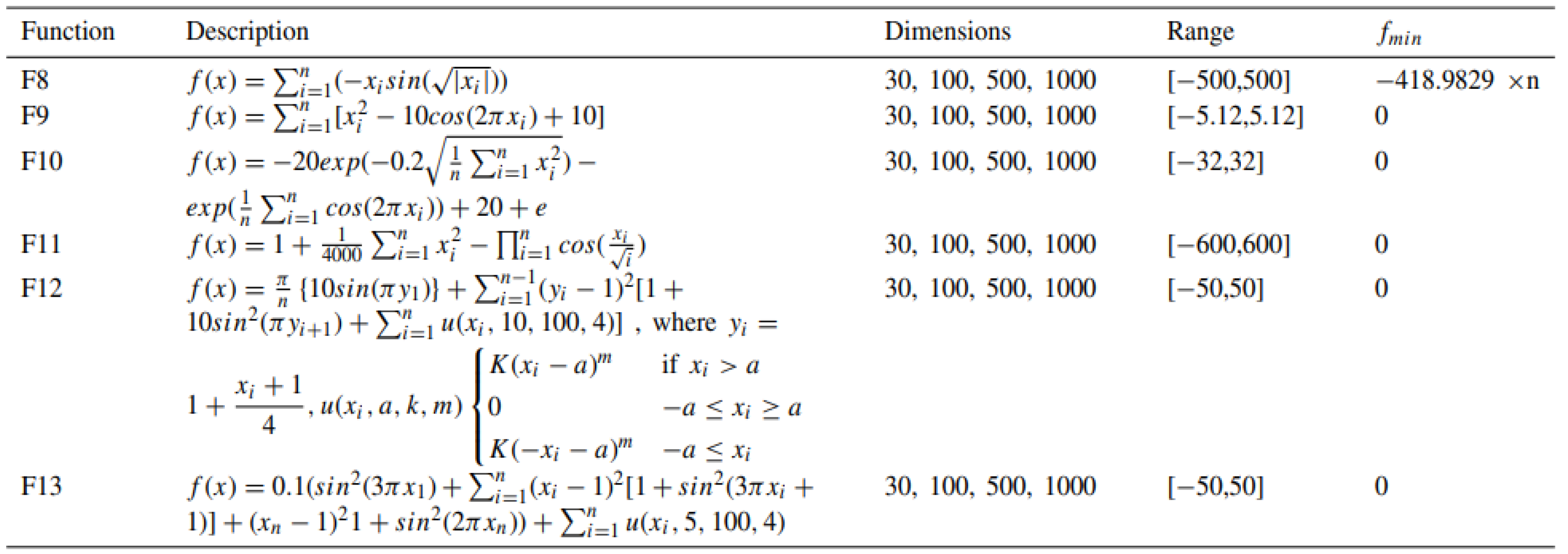
Table 4.
Fixed-dimension multimodal test functions.

Table 5.
Comparison of 30 times of differential evolution algorithm with crossover probability of 0.1 and 0.5.
Table 5.
Comparison of 30 times of differential evolution algorithm with crossover probability of 0.1 and 0.5.
| F | DE = 0.1) |
The DE used by Abualigahet al. [18] = 0.5) |
|---|---|---|
| F1 | 1.38E-03 | 1.33E-03 |
| F2 | 1.88E-04 | 6.83E-03 |
| F3 | 1.59E-01 | 3.97E+04 |
| F4 | 4.19E+01 | 1.15E+01 |
| F5 | 1.03E-01E | 1.06E+02 |
| F6 | 1.08E-04 | 1.44E-03 |
| F7 | 1.35E+01 | 5.24E-02 |
| F8 | -1.26E+04 | -6.82E+03 |
| F9 | 3.34E+01 | 1.58E+02 |
| F10 | 1.04E-02 | 1.21E-02 |
| F11 | 1.00E+00 | 3.52E-02 |
| F12 | 1.04E-06 | 2.25E-05 |
| F13 | 1.09E-13 | 9.12E-03 |
| F14 | 9.98E-01 | 1.23E+00 |
| F15 | 1.55E-03 | 5.63E-04 |
| F16 | -1.03E+00 | -1.03E+00 |
| F17 | 3.98E-01 | 3.98E-01 |
| F18 | 3.00E+00 | 3.00E+00 |
| F19 | -2.01E+00 | -3.86E+00 |
| F20 | -3.27E+00 | -3.27E+00 |
| F21 | -5.05E+00 | -8.65E+00 |
| F22 | -5.08E+00 | -9.75E+00 |
| F23 | -5.12E+00 | -1.05E+00 |
| No1 Rank | 15 | 12 |
Note: No.1 Rank is the number of times of getting the first place.
Table 6.
Parameter settings of the comparison algorithm(Abualigah et al. [18]).
Table 6.
Parameter settings of the comparison algorithm(Abualigah et al. [18]).
| Algorithm | Parameter | Value |
|---|---|---|
| PSO | Topology Cognitive and social constant Inertia weight Velocity limit |
Fully connected (C1, C2) 2, 2 Linear reduction from 0.9 to 0.1 10% of dimension range |
| CS | 0.25 | |
| BBO | Probability of modifying a habitat Probability limits of immigrations Size of each step I and E Probability of mutation |
1 [0, 1] 1 1 0.005 |
| DE | Scaling factor Crossover probability |
0.5 0.1 |
| GSA | Alpha, G0, Rnorm, Rpower | 20, 100, 2, 1 |
| FA |
|
0.5 0.2 1 |
| GA | Type Selection Crossover Mutation |
Real coded Roulette wheel (Proportionate) Whole arithmetic (Probability = 0.8, α = [−0.5, 1.5]) Gaussian (Probability = 0.05) |
| MFO | b | [−2 −1] 1 |
| GWO | Convergence parameter (a) | Linear reduction from 2 to 0 |
| BAT |
A r |
0 2 0.5 0.5 |
| FPA | Probability switch p | 0.8 |
| AOA |
|
5 0.5 |
Table 7.
Twelve improved differential evolution algorithms are applied to the unimodal functions .

Table 8.
Twelve improved differential evolution algorithms are applied to the multimodal test function.
Table 8.
Twelve improved differential evolution algorithms are applied to the multimodal test function.

Table 9.
Twelve improved differential evolution algorithms are applied to fixed-dimensional multimodal test functions.
Table 9.
Twelve improved differential evolution algorithms are applied to fixed-dimensional multimodal test functions.

Table 10.
The number of first rankings and average rankings of each algorithm.
| Algorithm | Total Average Rank | Total No1 Rank |
|---|---|---|
| AOA | 1.5217 | 15 |
| GWO | 3.1739 | 7 |
| FA | 4.1739 | 4 |
| CS | 4.2174 | 5 |
| DE | 4.6522 | 9 |
| BBO | 5.8696 | 3 |
| FPA | 6.3478 | 5 |
| MFO | 6.5217 | 4 |
| GA | 7.5217 | 2 |
| PSO | 8.7391 | 2 |
| GSA | 9.6957 | 0 |
| BAT | 10.0870 | 1 |
Note: No.1 Rank is the number of times of getting the first place; Average Rank is the average of the rankings.
Table 11.
Twelve improved differential evolution algorithms, DE and MBDE are applied to the Unimodal test functions.
Table 11.
Twelve improved differential evolution algorithms, DE and MBDE are applied to the Unimodal test functions.

Table 12.
Twelve improved differential evolution algorithms, DE and MBDE are applied to the Multimodal test functions.
Table 12.
Twelve improved differential evolution algorithms, DE and MBDE are applied to the Multimodal test functions.

Table 13.
Twelve improved differential evolution algorithms, DE and MBDE are applied to fixed-dimensional multimodal test functions.
Table 13.
Twelve improved differential evolution algorithms, DE and MBDE are applied to fixed-dimensional multimodal test functions.

Table 14.
The number of first places and the average ranking of twelve improved differential evolution algorithms and DE and MBDE.
Table 14.
The number of first places and the average ranking of twelve improved differential evolution algorithms and DE and MBDE.
| Algorithm | Total Average Rank | Total No1 Rank |
|---|---|---|
| IHDE-BPSO3 | 1.2381 | 18 |
| MBDE2 | 1.2381 | 18 |
| IHDE2 | 1.7619 | 18 |
| MBDE | 2.0000 | 18 |
| IHDE-BPSO5 | 2.0476 | 18 |
| IHDE-2cross | 2.0952 | 18 |
| IHDE-BPSO4 | 2.0952 | 18 |
| IHDE-HPSO5 | 2.2381 | 18 |
| DE | 2.8571 | 18 |
| IHDE | 2.9524 | 16 |
| IHDE-HPSO4 | 3.4286 | 16 |
| IHDE-mbi | 3.4762 | 16 |
| IHDE-mbm | 3.5714 | 16 |
| IHDE-HPSO3 | 3.7143 | 15 |
Note: No.1 Rank is the number of times of getting the first place; Average Rank is the average of the rankings.
Disclaimer/Publisher’s Note: The statements, opinions and data contained in all publications are solely those of the individual author(s) and contributor(s) and not of MDPI and/or the editor(s). MDPI and/or the editor(s) disclaim responsibility for any injury to people or property resulting from any ideas, methods, instructions or products referred to in the content. |
© 2025 by the authors. Licensee MDPI, Basel, Switzerland. This article is an open access article distributed under the terms and conditions of the Creative Commons Attribution (CC BY) license (http://creativecommons.org/licenses/by/4.0/).
Copyright: This open access article is published under a Creative Commons CC BY 4.0 license, which permit the free download, distribution, and reuse, provided that the author and preprint are cited in any reuse.